Theoretical Study of Path Adaptability Based on Surface Form Error Distribution in Fluid Jet Polishing

Abstract

In the technology of computer-controlled optical surfacing (CCOS), the convergence of surface form error has a close relationship with the distribution of surface form error, the calculation of dwell time, tool influence function (TIF) and path planning. The distribution of surface form error directly reflects the difference in bulk material removal depth across a to-be-polished surface in subsequent corrective polishing. In this paper, the effect of path spacing and bulk material removal depth on the residual error have been deeply investigated based on basic simulation experiments excluding the interference factors in the actual polishing process. With the relationship among the critical evaluation parameters of the residual error (root-mean-square (RMS) and peak-to-valley (PV)), the path spacing and bulk material removal depth are mathematically characterized by the proposed RMS and PV maps, respectively. Moreover, a variable pitch path self-planning strategy based on the distribution of surface form error is proposed to optimize the residual error distribution. In the proposed strategy, the influence of different bulk material removal depths caused by the distribution of surface form error on residual error is compensated by fine adjustment of the path spacing according to the obtained path spacing optimization models. The simulated experimental results demonstrate that the residual error optimization strategy proposed in this paper can significantly optimize the overall residual error distribution without compromising the convergence speed. The optimized residual error distribution obtained in sub-regions of the polished surface is more uniform than that without optimization and is almost unaffected by the distribution of parent surface form error.

1. Introduction

Whether it is in the high-end fields such as the defense industry, aviation and aerospace, or in the civilian fields of medical devices, mobile phones, cameras, etc., high-precision optical components are playing an increasingly important role. At the same time, there are increasingly higher requirements for surface form error, medium frequency error, surface roughness and subsurface damage of optical components [1]. With the introduction of aspherical and free form surface design methods, precision devices composed of optical components have been unified in terms of portability and functionality. However, this also poses a great challenge to the ultra-precision machining of optical components. Ultra-precision grinding and deterministic polishing are the main means of processing ultra-precision optical components [2]. Traditional manual polishing has the disadvantages of high labor intensity, poor working environment, being time consuming, high dependence on workers’ experience, difficulty in controlling the consistency of quality, etc. [3]. Automated polishing is inevitably a trend to replace manual polishing. Computer-controlled optical surfacing technology (CCOS), first proposed by Itek. Inc. in 1970, has been widely used and developed in optical surfacing with high form accuracy [4,5].

In recent years, with the development of a series of advanced non-traditional sub-aperture CCOS polishing technologies such as bonnet polishing [6], fluid jet polishing [7], magnetorheological polishing [8], ion beam polishing [9], laser polishing [10], etc., the controllability of deterministic polishing has taken a new step, which provides more possibilities for the improvement of the correction effect of the surface form error. Among them, fluid jet polishing is an ultra-precise finishing technology that combines fluid mechanics, precision manufacturing and surface engineering. In this polishing technology, the fluid is used as a carrier for the abrasive particles suspended within, forming a flexible polishing head that acts on the workpiece surface with a good fit and gets rid of tool wear issues altogether. Therefore, this technology has a strong adaptability to complex free form shapes and is especially suitable for the ultra-precision polishing of optical lenses, mirrors and molds made of hard and brittle materials. In addition, fluid jet polishing in the general submerged polishing case and some non-submerged polishing cases with narrow sapphire nozzles (with a diameter less than 0.3 mm) can generate tool influence function (TIF) with a small radius and a Gaussian or near Gaussian distribution. These advantages make fluid jet polishing a strong technology to achieve precise correction of the surface form error.

In the technology of CCOS, the convergence of surface form error has a close relationship with the distribution of surface form error, calculation of dwell time, tool influence function (TIF) and path planning. In practice, after measurement of the workpiece to be polished, the resulting surface form error can be generally expressed as a continuously changing free form surface. The optimal distribution of residual error after deterministic polishing should be as close to an ideal plane as possible and ensure sufficient convergence accuracy. However, the distribution of surface form error directly brings a difference in bulk material removal depth across a to-be-polished surface in subsequent corrective polishing. After the surface has been polished with a traditional path with a fixed pitch, it can be seen that the residual error distribution after deterministic polishing is largely affected by the distribution of parent surface form error. In this paper, this phenomenon is identified as a genetic phenomenon of error distribution. This makes it difficult to ensure the consistency of the accuracy in the entire region of the workpiece after ultra-precision polishing, and it also brings difficulties for subsequent iterations of corrective polishing. Therefore, on the premise of not affecting the degree of convergence, after every corrective polishing iteration in the pre-polishing stage, the residual error distribution that is more uniform and almost free from the influence of the parent surface form error distribution should be obtained as much as possible, which is of great theoretical significance and engineering value.

The mid-spatial-frequency (MSF) error, i.e., the ripple error of optical components, has an important impact on the performance of laser systems and high quality imaging systems. At present, some scholars mainly have been focusing on the suppression of ripple error. However, there is not much research on the genetic phenomenon of the error distribution and its relationship with ripple error. When using jet polishing to correct the surface with a large difference in surface form error, Li et al. proposed a selective region path planning strategy to optimize the residual error distribution and successfully avoided the introduction of path error in the region where the surface form accuracy meets the requirements [11]. The influencing factors of ripple error mainly include initial surface error, TIF and polishing path. In terms of the polishing path, the ripple error can be suppressed by changing the randomness of the path to optimize the period of the ripple error and choosing a reasonable path spacing to optimize the height of the ripple error [12]. Dunn et al. [13], Wang et al. [14] and Takizawa et al. [15] proposed the six-direction, four-direction and circular pseudo-random paths, respectively. Their experimental results showed that the random variability of the path direction can effectively suppress the MSF error. In the deterministic surface correction process, a small path spacing should generally be preferred. Too large a path spacing is not conducive to correcting the surface form error and suppressing the ripple error. However, due to changes in material removal and the speed limitation of the axes of the polishing machine, polishing along an overly-dense path will introduce additional dwell time and cause excessive material removal, especially in regions where material removal is low, which is unfavorable for the convergence of surface accuracy. Wang et al. proposed to use the inflection point of the approximately reversed “L”-shaped curve between path spacing and ripple error to determine the optimal path spacing, which provides a fast and efficient method for optimal selection of path spacing [16]. Hou et al. proposed to divide the surface into several regions from the perspective of suppressing the MSF error and plan polishing paths with different pitches in different form error regions [17]. In their implementation process, the transition of polishing paths in different regions and the avoidance of the path edge effect are complicated. Hu et al. also proposed a polishing path with random spacing based on the distribution of surface form error [18]. Their choice of path spacing is based on empirical formulas, and the intrinsic relationship between form error and path spacing has not been studied in depth.

In this paper, the influence law of path spacing and bulk material removal depth on residual error is deeply studied. It is not difficult to understand that the influence law of the distribution of surface form error on residual error can be revealed by studying the effects of different bulk material removal depths on residual error. On this basis, mathematical modeling is used to demonstrate the feasibility of the novel idea consisting of the normalizing residual error distribution by optimizing the path spacing under the condition that other polishing conditions including TIF are unchanged. This idea considers the fine adjustment of the path spacing to compensate for the effect of the surface form error on the residual error. A complete residual error optimization strategy based on the form error distribution is proposed. During the implementation of this optimization strategy, according to the established path spacing optimization model and the actual surface form error distribution of the workpiece to be polished, the corresponding variable pitch polishing path with seamless transition is planned for polishing, thereby optimizing the residual error distribution and greatly reducing the influence of the parent form error distribution on the child residual error distribution.

The contents of this paper are organized as follows. Section 2 describes the convolution removal principle in CCOS and the fast solution algorithm for the dwell time based on linear equations. Section 3 deeply studies and analyzes the influence of path spacing and bulk material removal depth on residual error. In Section 4, the residual error optimization strategy based on root-mean-square (RMS) and the peak-to-valley (PV) map is proposed. In this strategy, the corresponding path spacing optimization model and variable pitch path planning method are described, respectively. Section 5 makes a comparative study of optimization strategies, and Section 6 concludes the full text.

2. Theoretical Background

2.1. Convolution Removal Principle in Computer-Controlled Optical Surfacing

The deterministic polishing material removal process can be viewed as a two-dimensional convolution of the TIF and dwell time. The surface form error can be obtained by comparing the actual measured surface data with the ideal surface data and using filtering and other technical means to eliminate the middle-to-high-spatial frequency component and retain the low-spatial frequency component. The deterministic polishing process can precisely control the dwell time of the polishing tool at each dwelling point according to the obtained surface form error and the planned polishing path, thereby realizing different amounts of material removal at different positions, which can not only improve the accuracy of the surface, but also enhance the surface quality. In general, the above process is implemented by converting calculated dwell time to feed rate of the polishing tool, which is an iterative process. The convolution material removal and resulting residual error for each iteration can be expressed by Equation (1) as follows:

$$\left\{\begin{array}{c}Z\left(x,y\right)=R\left(x,y\right)\otimes D\left(x,y\right)\hfill \\ E\left(x,y\right)=Z_0\left(x,y\right)-Z\left(x,y\right)\hfill \end{array}\right.$$

(1)

where $Z(x,y)$ represents the convolution material removal; $R(x,y)$ represents the material removal function per unit time; $D(x,y)$ stands for the dwell time function; $E(x,y)$ represents the residual error after deconvolution removal; $Z_0(x,y)$ represents the surface form error that is expected to be removed.

2.2. Dwell Time Solution Based on Linear Equations

According to Equation (1), given the material removal map and material removal function, the solution of the dwell time can be regarded as a deconvolution process, and its solution algorithm has an important effect on the deterministic polishing process and results. Existing dwell time algorithms are mainly split into two categories: discrete convolution model and linear equation model. The former has a fast computation speed, but usually low convergence accuracy. The latter has high accuracy, but the solution speed is slow. With the introduction of regularization and sparse matrix operation, the solution algorithm based on the linear equation model is becoming more stable and fast, and it can be applied to a flexible and changeable planning path, which makes it more feasible and flexible in practical application [19]. It is assumed that there are n dwell points along the planned path on the to-be-polished surface; the surface is divided into m control points; and correction of the surface is simplified to reduce the form error at these control points. When the TIF dwells at a dwell point, the material removal at all control points within a unit of time can be written in the form of $m\times 1$, and then, the TIF removal matrix $A_{m\times n}$ for the n dwell points can be obtained, which is usually a sparse matrix with m rows and n columns. The form error to be removed at the m control points is represented as a column $b_m\times 1$. Similarly, the dwell time of each dwell point to be calculated is also written as a column vector form, i.e., $x_n\times 1$. In the linear model solution, the dwell time corresponding to each dwell point can be estimated by solving the equation $A_{m\times n}{x}_{n\times 1}=b_{m\times 1}$. However, because it is an indefinite equation and the large condition number means that rounding error and other errors will seriously affect the solution of the problem, the regularization method using the smart damping factor is used here to ensure stability of the solution, as shown in Equation (2) [20].

$$\left\{\begin{array}{c}\left(\begin{array}{c}{A}_{m\times n}\\ \gamma \times E_{m-n}\end{array}\right)x_{n\times 1}=\left(\begin{array}{c}{b}_{m\times 1}\\ 0\times I_{\left(m-n\right)\times 1}\end{array}\right)\hfill \\ \gamma =3\times TRP\hfill \end{array}\right.$$

(2)

where $\gamma$ represents the regularized damping coefficient, $E_{m-n}$ represents a unit matrix of $(m-n)$ order and $I_{(m-n)\times 1}$ represents a column vector containing $(m-n)$ elements. $TRP$ represents the maximum removal depth of the TIF per unit time, in $\lambda$/min ($\lambda$ = 632.8 nm).

By using the least squares method and sparse matrix method to solve the objective function of Equation (3), the stable and reliable solution of dwell time can be obtained.

$$min\left\{{∥Ax-b∥}^2+{∥\gamma x∥}^2\right\},x\ge 0$$

(3)

3. Research on the Effect of Path Spacing and Bulk Material Removal Depth on Residual Error

The actual polishing experiment is more or less affected by various interference factors such as clamping error and stability of the polishing liquid, which make it difficult to extract separately the influence of path spacing and bulk material removal depth on residual error. This section proposes the use of simulation experiments to investigate the laws of influence among them. A similar polishing simulation method can effectively eliminate the interference of other factors and greatly saves time and money.

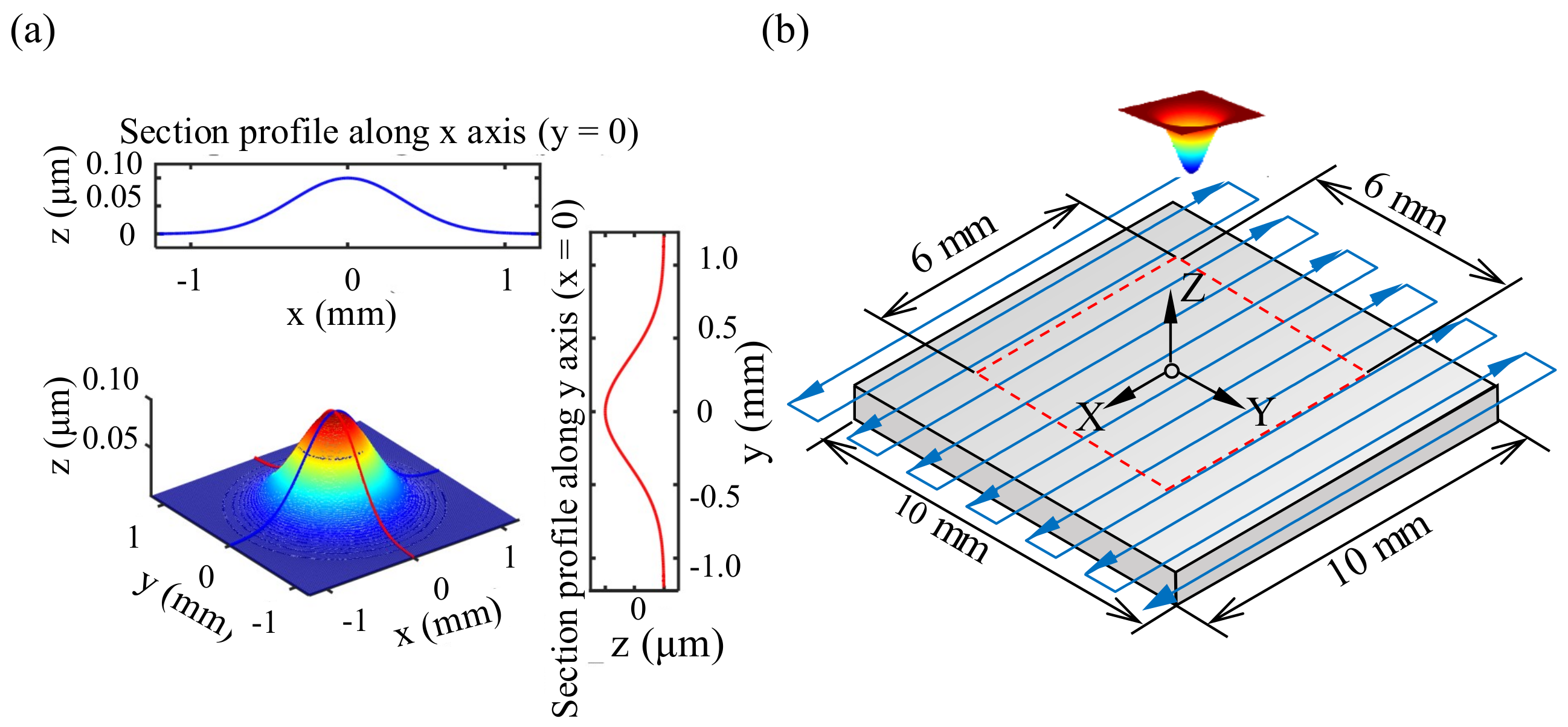
3.1. Simulation Experiment Design

In submerged jet polishing (for narrow sapphire nozzles with a diameter less than 0.3 mm) and other deterministic polishing, the TIF usually presents a Gaussian distribution with a maximum removal at the center. In the simulation study of this paper, the TIF established by the Gaussian mathematical model given in Equation (4) is used, where $R_x$ and $R_y$ represent the material removal area radius (mm) of the TIF in the x direction and the y direction, respectively. a represents the maximum material removal depth per unit time ($\mathsf{\mu }$m/min). Figure 1a shows the rotationally-symmetric three-dimensional TIF profile with a removal radius of 1 mm and a maximum removal depth of $0.1\mathsf{\mu }$m/min.

Table 1. The parameter values of tool influence function (TIF).

Parms	a ($\mathsf{\mu }$/min)	$R_x$ (mm)	$R_y$ (mm)
Values	0.1	1.0	1.0

gives the parameter values of the TIF used in this paper.

$$\left\{\begin{array}{c}sigmax=R_x/2\sqrt{2},sigmay=R_y/2\sqrt{2}\hfill \\ z=a\times e^{-\left(x^2/\phantom{x^2\left(2sigmax\right)}\left(2sigmax\right)+y^2/\phantom{y^2\left(2sigmay\right)}\left(2sigmay\right)\right)}\hfill \\ TRP=a\times {10}^3/\phantom{a\times {10}^3\lambda }\lambda ,\lambda =632.8\mathrm{nm}\hfill \end{array}\right.$$

(4)

Without loss of generality, a scanning path was planned on a planar specimen with a length of 10 mm and a width of 10 mm, and the deterministic polishing simulation was implemented according to the given TIF, as shown in Figure 1b. Since it is difficult for the computer to achieve continuous removal in simulations, in order to make the discrete removal simulation more closely approximate the continuous removal commonly used in actual polishing, the number of dwell points along the planned path was increased. Here, the distance between adjacent dwell points along the path was set to 0.05 mm. The simulation results in our test show that the actual continuous polishing removal can be well approximated. The RMS and PV values of the residual error obtained after correction were used as evaluation indexes for the deterministic polishing convergence accuracy and the removal effect. In addition, the power spectral density (PSD) method was used to analyze the MSF error component in the residual error and study the effect of path spacing and surface form error on the component. In order to avoid the influence of edge effect in the simulation process, the central region of the specimen with a length of 6 mm and width of 6 mm served as a residual error evaluation region.

In order to deeply study the influence of path spacing and bulk material removal depth on the residual error obtained after polishing, three groups of basic simulation experiments were carefully designed. The first set of experiments studied the effect of path spacing on residual error under fixed bulk material removal depth. The second set of experiments investigated the effect of bulk material removal depth on the residual error in the case of fixed path spacing. The third set of experiments investigated the effect of path spacing variations on the residual error resulting from different bulk material removal depths.

Table 2. Simulation experiment conditions.

Experiment Set	Path Pitch (mm)	Bulk Material Removal Depth ($\mathsf{\mu }$m)
Exp. 1	0.1 , 0.2, 0.3, ... , 2.5	0.5
Exp. 2	0.2	0, 0.1, 0.2, ... , 1.0
Exp. 3	0.1, 0.2, 0.3, ... , 2.5	0, 0.1, 0.2, ... , 1.0

gives details of the experimental conditions for the three simulation experiments.

3.2. Simulation Results and Analysis

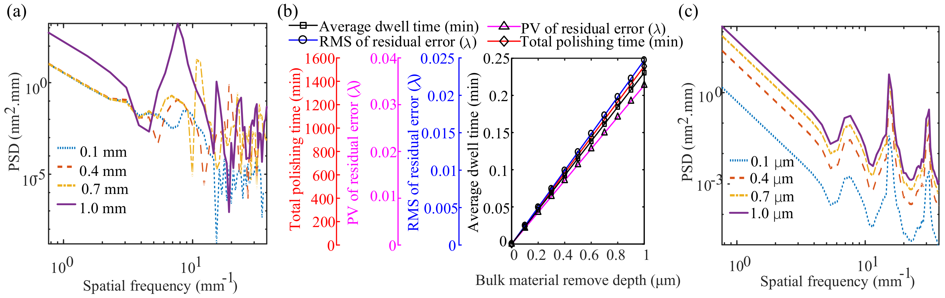
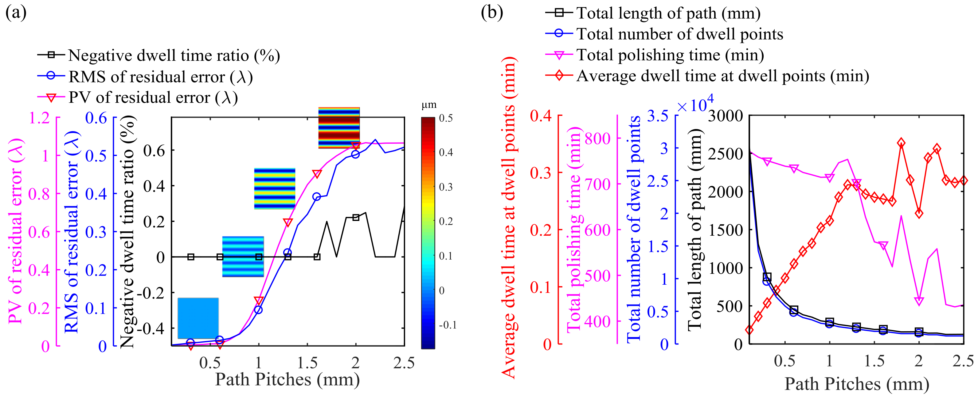
3.2.1. Influence of Path Spacing on Residual Error

By introducing regularization and sparse matrix operation methods, the dwell time solution algorithm based on the linear equations can effectively control the negative ratio (number of dwell points with a negative dwell time calculated/total number of dwell points) of dwell time calculated to be less than 1%, as shown in Figure 2a. Note that the influence of path spacing on the RMS and PV values of the residual error is almost consistent when bulk material removal depth is constant. As the path spacing increases, the RMS and PV values of the residual error first increase slowly and approximately linearly within the range of 0.1 mm to 0.6 mm, then rapidly increase within the range of 0.6 mm to 2.0 mm and finally stabilize in the range of 2.0 mm to 2.5 mm. This is because the deterministic polishing removal is caused by the convolution effect formed by the overlap of tool influence functions. When the distance between the paths is small, i.e., less than 3/10 of the diameter of the TIF, convergence of the deterministic polishing removal process can be effectively ensured. From the residual error profile in Figure 2a, it can be seen that as the path spacing increases, it becomes increasingly difficult to ensure convergence of the regions between adjacent paths. When the distance between the paths is larger than the diameter of the TIF, the material between the adjacent paths cannot be removed. In this case, the PV values of the residual error will be slightly larger than the original surface form error and remain basically constant. However, it should be pointed out that the RMS curve is fluctuating more at these later stages than the PV curve. This may be because the RMS value of the residual error is more susceptible to dramatic changes in convergence of the surface form error.

Figure 2b shows that as path spacing increases, the total length of the path is drastically shortened, but the total polishing time is only slightly reduced within the path range of 0.1 mm to 1.0 mm. The polishing time for deterministic polishing is mainly determined by the TIF and volume of material removal. More polishing time means more volume removal. The error of a certain control point basically determines the total dwell time at that point. As the path spacing decreases, although the path length increases sharply, the number of dwell points increases at the same time, and the average dwell time allocated to each dwelling point will be reduced accordingly, so that the total polishing time remains basically unchanged. In addition, considering that as the path spacing increases, the degree of convergence of deterministic polishing decreases, the overall material removal will be reduced, and thus, the polishing time will tend to decrease. When the path spacing is greater than 1.0 mm, the degree of convergence of the polishing removal sharply changes and shows a downward trend, so that the total polishing time is drastically reduced with a certain degree of fluctuation.

Figure 3a shows the power spectral density curve of the residual error calculated along the y-direction, which is the perpendicular direction of the planned path when the path distance is 0.1 mm, 0.4 mm, 0.7 mm and 1.0 mm, respectively. It can be seen that as the path spacing increases, the MSF error becomes larger and larger, which is mainly due to waviness error caused by the tool path. It can be concluded that for deterministic polishing removal, a small path spacing should be preferred, which can effectively reduce the RMS and PV values of the residual error and effectively suppress the MSF.

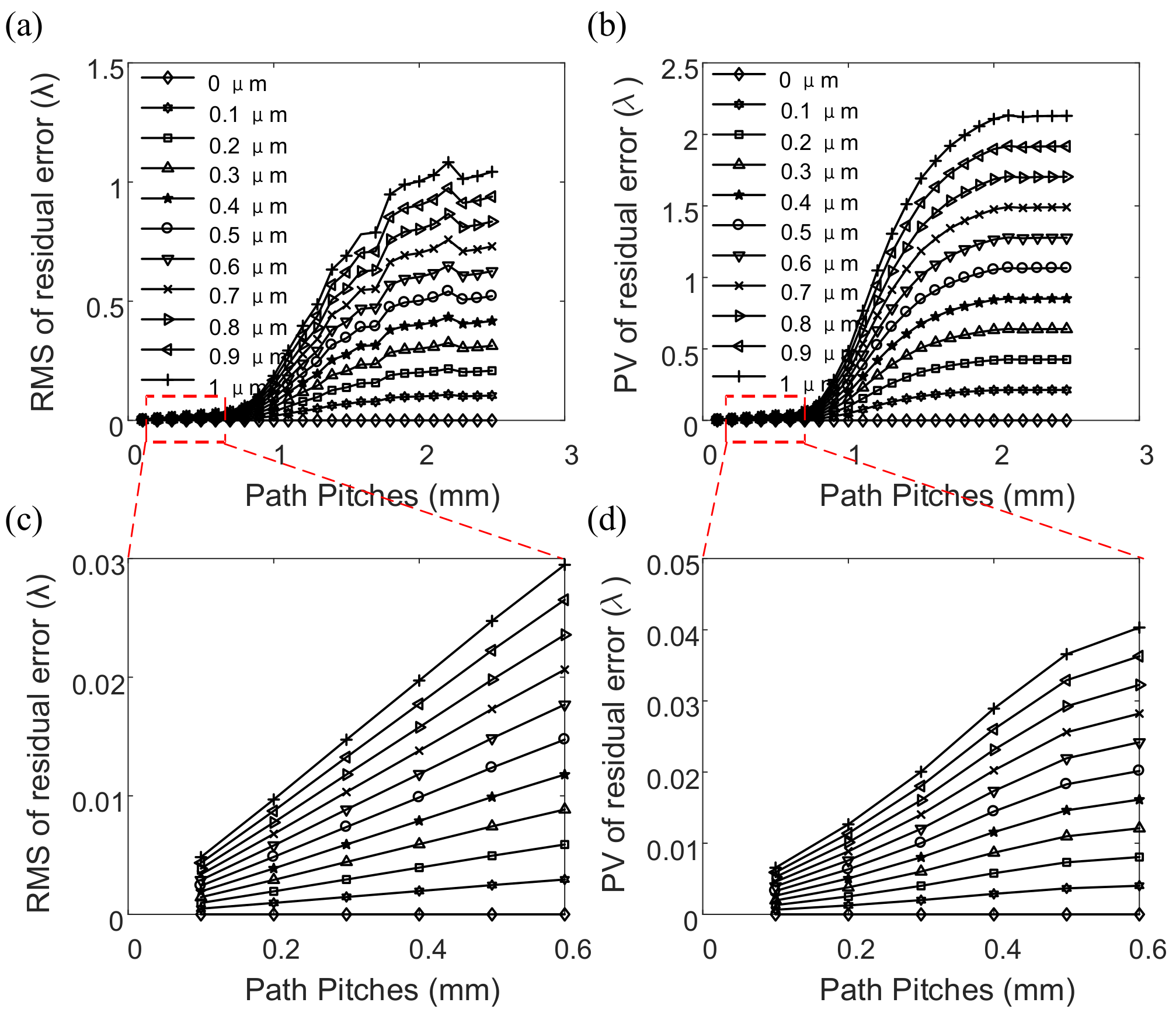
3.2.2. Influence of Bulk Material Removal Depth on Residual Error

Figure 3b shows the influence of the bulk material removal depth on the residual error when the path spacing is constant. With the increase of bulk material removal depth, RMS and PV values of the residual error showed a linear growth trend. This also reflects the linear decreasing trend of convergence of deterministic polishing with the increase of the bulk material removal depth. With the increase of the bulk material removal depth, the linear increase of the polishing time indicates that polishing time has a positive correlation with the amount of material removal. Since the number of pre-planned dwell points remains constant, the average dwell time allocated to each dwell point increases accordingly. Figure 3c shows the power spectral density calculation results for the residual error along the vertical direction of the planned path for different bulk material removal depths (0.1 $\mathsf{\mu }$m, 0.4 $\mathsf{\mu }$m, 0.7 $\mathsf{\mu }$m, 1.0 $\mathsf{\mu }$m) when the path pitch is 0.2 mm. It can be seen that the profiles of the power spectral density curve corresponding to different bulk material removal depths are similar, but as the bulk material removal depth increases, the power density amplitude corresponding to each spatial frequency shows a significant increase. This may be because with the increase of the bulk material removal depth, the dwell time of each dwell point is prolonged. The increase in the dwell time of the polishing tool at a certain point will make the path effect more pronounced, thereby introducing deeper ripple errors caused by the tool path. Therefore, for a large form error, a small path spacing should be preferred, which can effectively improve the convergence of deterministic removal, reduce the RMS and PV value of the residual error and effectively suppress the MSF error component in the residual error.

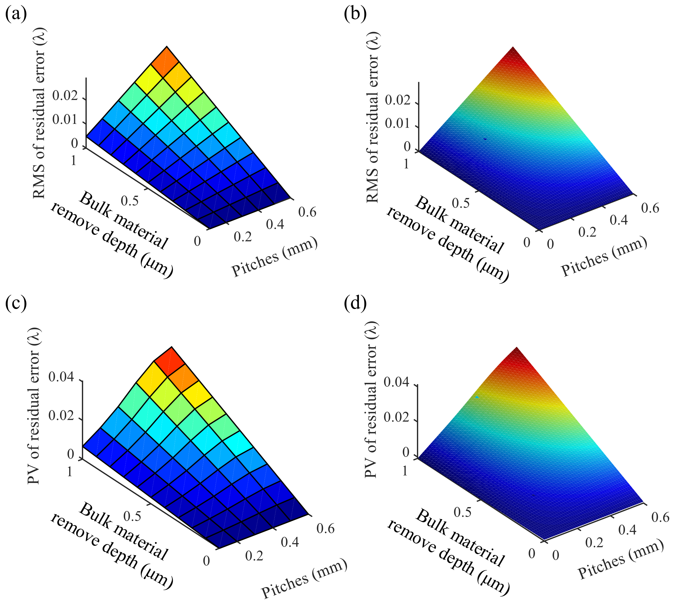
3.2.3. Effect of Path Spacing Variations on the Residual Error Resulting from Different Bulk Material Removal Depths

As can be seen from Figure 4a,b, the influence law of path spacing variations on the RMS and PV values of residual error resulting from different bulk material removal depth is consistent. For deterministic polishing removal, a reasonable polishing path spacing value should be less than 3/10 of the diameter of the TIF. When the value is within this range, drastic variation of RMS and PV values of the residual error can be effectively avoided. Therefore, in this simulation, the RMS and PV curves with a path pitch of less than 0.6 mm are the parts of interest. As can be seen from the partially enlarged view, shown in Figure 4c,d, the slope of the curve increases significantly with the increase of the form error. This indicates that the larger the bulk material removal depth, the greater the effect of the change in the path spacing on the residual error, which makes the subsequent adjustment of the path spacing more useful, especially for regions with large bulk material removal depth.

3.3. Summary and Discussion of Simulation Results

Through the above three sets of simulation experiments, the influence rules of path spacing and bulk material removal depth on the residual error obtained after deterministic polishing were thoroughly studied and analyzed. When the path spacing was fixed, the larger the bulk material removal depth, the larger the RMS and PV values of residual error. The distribution of surface form error directly reflected the difference in bulk material removal depth across a to-be-polished surface in subsequent corrective polishing. This is a good explanation of the genetic phenomenon of the error distribution during the surface correction process. In the case where the bulk material removal depth was constant, the path spacing also affected the RMS and PV values of residual error approximately linearly. Once the surface form error distribution of the actual workpiece was determined, we could get the variation in bulk material removal depth across the surface and could consider the use of fine-tuning of the path spacing to compensate for the effect of surface form error on the residual error, as well as achieve the purpose of optimizing the residual error distribution. That is to say, small path spacing was used where surface form error was large, and a large path spacing was used where surface form error was small, so that the path spacing adapted to the variation of the surface form error, which was expected to make the optimized residual error distribution obtained more uniform and almost unaffected by the distribution of parent surface form error.

4. Residual Error Optimization Strategy Based on Root-Mean-Square and Peak-to-Valley Maps

Based on results of the simulation experiment in Section 3, it can be seen that the RMS and PV values of the residual error after deterministic polishing are influenced by both the bulk material removal depth and the path spacing. This section aims to establish their relationship models with the path spacing and bulk material removal depth, respectively. To achieve this goal, this paper introduces the concept of RMS and PV maps for the first time and proposes a path spacing optimization model based on the above two maps in order to optimize the corresponding RMS and PV values of the residual error. The detailed flow for variable pitch spiral path planning in residual error optimization strategy is also given.

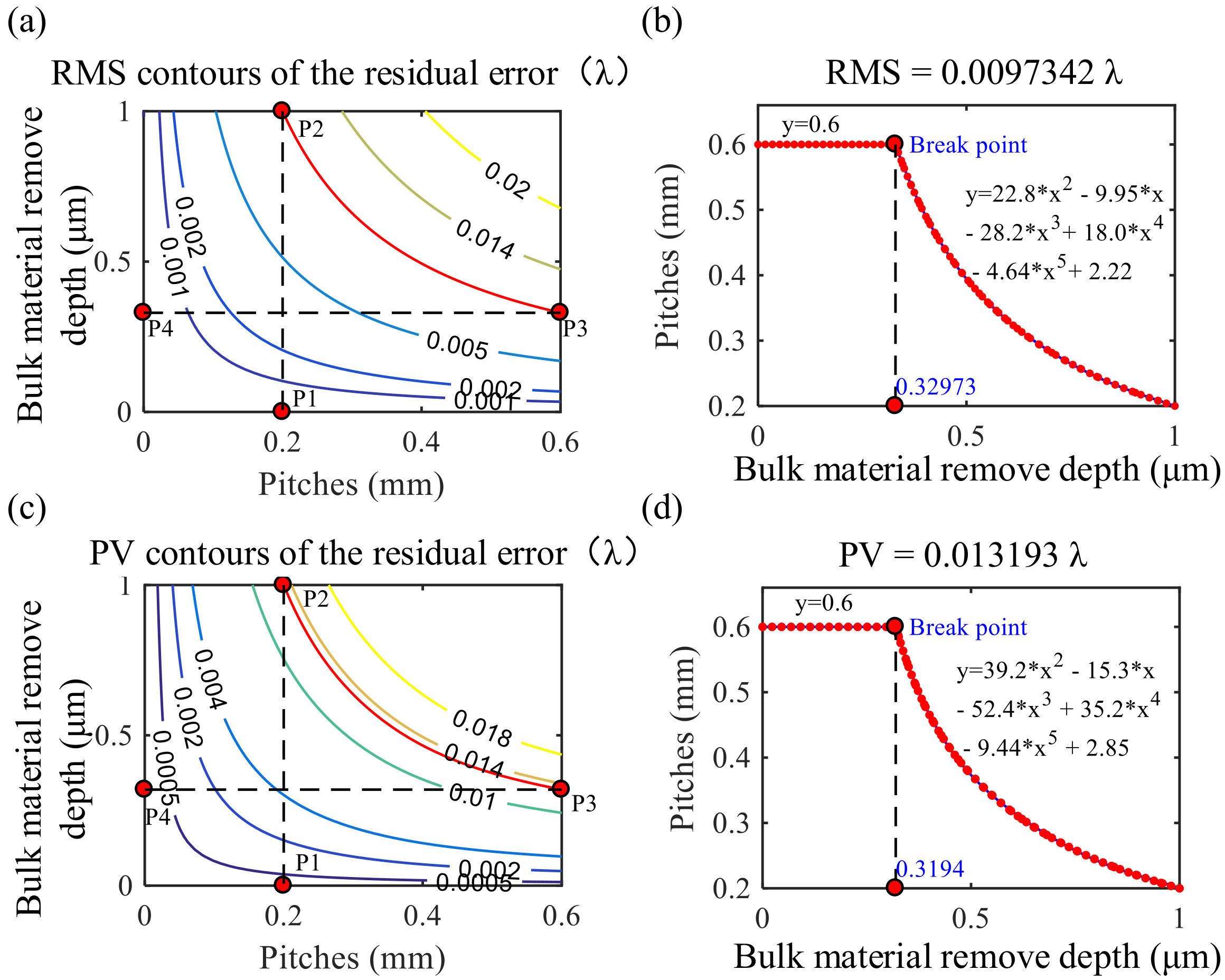
4.1. Derivation of the RMS and PV Maps

The RMS (PV) map characterizes the relationship of the RMS (PV) value of the residual error obtained after theoretical deterministic polishing with the path spacing and the surface form error. From the results of the third set of simulation experiments in Section 3, the experimental data in the range of reasonable path spacing (0.1 mm to 0.6 mm) were extracted and collated, and then, the initial RMS and PV maps were obtained, as shown in Figure 5a,c. Using surface fitting techniques, we obtained the final smoothed RMS and PV maps, as shown in Figure 5b,d. The proposed RMS and PV maps provide a theoretical model reference for predicting the RMS and PV values of the residual error after practical deterministic polishing.

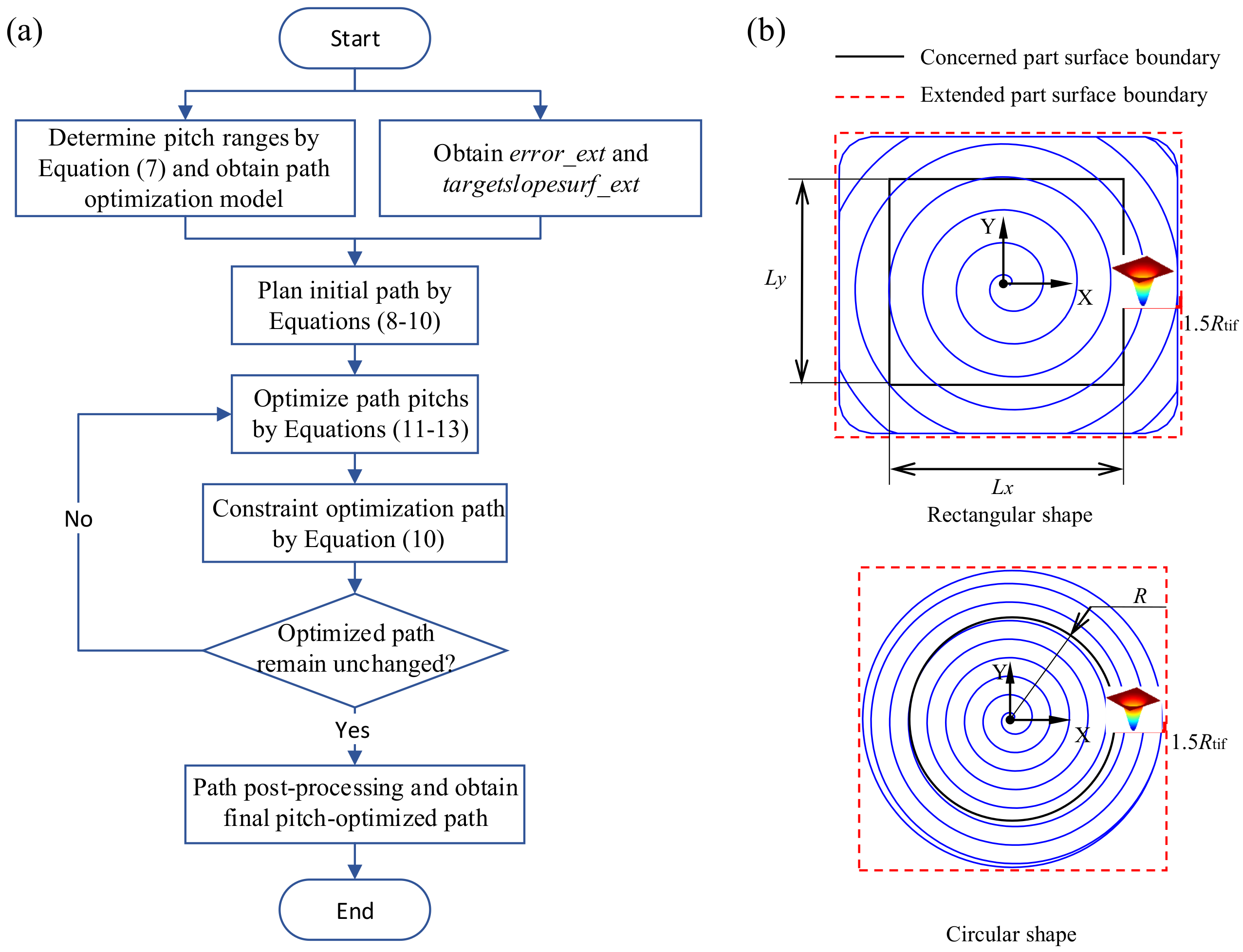
4.2. Path Spacing Optimization Model Based on Surface Form Error

Based on the RMS map of Figure 5b, the RMS contour of the residual error shown in Figure 6a is obtained. On the RMS contour, all points with the same RMS value form continuous curves in sequence. The curve reflects the correspondence between the bulk material removal depth to be corrected and path spacing for which the RMS value of residual error is controlled to be a constant value. Although corrective polishing should be preferably performed with a small path pitch, the path pitch in actual polishing cannot be set infinitely small. The variation range of expected bulk material removal depth in one polishing iteration is constant. As shown in Figure 6a, once the minimum path spacing is set, for the minimum path used in the region with largest bulk material removal depth, the theoretical optimum RMS value of the residual error after polishing is determined. Conversely, given the RMS value of the residual error we expect, we can get the corresponding minimum path spacing. Moreover, the smaller the RMS value of the desired residual error, the smaller the corresponding minimum path spacing. In the simulation experiments in this paper, the bulk material removal depth varies from 0.5 $\mathsf{\mu }$m to 1.0 $\mathsf{\mu }$m. We specify the minimum path spacing as $p_{\min }=0.2$ mm and the maximum path spacing is $p_{\max }=0.6$ mm. The P1 point determined by the minimum pitch gives the best RMS value of the residual error corresponding to key point P2, and then, the contour line of the best RMS value is located. The contour curve determines the point P3 at the position of the maximum path spacing. P3 determines the critical value of bulk material removal depth corresponding to point P4. When the bulk material removal depth of the region to be corrected is smaller than the critical value, the path spacing corresponding to the region should be set to the maximum path spacing. Finally, the relationship between the bulk material removal depth and the path spacing based on the RMS map is obtained, as shown in Figure 6b.

Similarly, the PV contour of residual error and the relationship between the bulk material removal depth and the path spacing based on the PV map are obtained, as shown in Figure 6c,d. A comparison of Figure 6b,d shows that the trend of the two curves is similar, which is attributed to the similarity of the effects of bulk material removal depth, and path spacing on the RMS and PV values of the residual error. A piecewise polynomial fitting method was used to fit the two curves, respectively, and the path spacing optimization models based on the RMS map (Equation (5)) and the PV map (Equation (6)) were obtained, respectively.

$$p_{rms}\left(z_h\right)=\left\{\begin{array}{c}0.6\hfill \\ -4.46{z_h}^5+18.0{z_h}^4-28.2{z_h}^3+22.8{z_h}^2-9.95z_h+2.22\hfill \end{array}\begin{array}{c},z_h<0.3297\\ ,z_h\ge 0.3297\end{array}\right.$$

(5)

$$p_{pv}\left(z_h\right)=\left\{\begin{array}{c}0.6\hfill \\ -9.44{z_h}^5+35.2{z_h}^4-52.4{z_h}^3+39.2{z_h}^2-15.3z_h+2.85\hfill \end{array}\begin{array}{c},z_h<0.3194\\ ,z_h\ge 0.3194\end{array}\right.$$

(6)

in which $z_h$ stands for the bulk material removal depth ($\mathsf{\mu }$m); $p_{rms}$, $p_{pv}$ represent the resulting path spacing (mm) based on the RMS-map optimization model and the PV-map optimization model, respectively.

It is important to point out that several simulation experiments have shown that when the fluctuation range of the parent surface form error is large, expectations for the degree of residual error optimization should be reduced in one iteration, and the minimum path spacing should be selected to be larger, thereby increasing the critical value of bulk material removal depth determined by point P4 and reducing the variation range of the polishing path pitch. This is more conducive to reducing the impact of the distribution of the parent surface form error on the child residual error distribution, while avoiding distortion of the planned variable pitch path and affecting the final polishing effect. Equation (7) gives the empirical formula for the choice of minimum and maximum path spacing under the same parameters of the optimization strategy proposed in this paper.

$$\left\{\begin{array}{c}{p}_{max}=3R_{tif}/\phantom{3R_{tif}5}5\hfill \\ p_{min}=2p_{max}\times \left[max\left(Z_0\left(x,y\right)\right)-min\left(Z_0\left(x,y\right)\right)\right]/\phantom{2p_{max}·\left[max\left(Z_0\left(x,y\right)\right)-min\left(Z_0\left(x,y\right)\right)\right]\left(3max\left(Z_0\left(x,y\right)\right)\right)}\left(3max\left(Z_0\left(x,y\right)\right)\right)\hfill \end{array}\right.$$

(7)

where $R_{tif}$ represents the radius of the TIF; max($Z_0(x,y)$) and min($Z_0(x,y)$) represent the largest and the smallest form error, respectively.

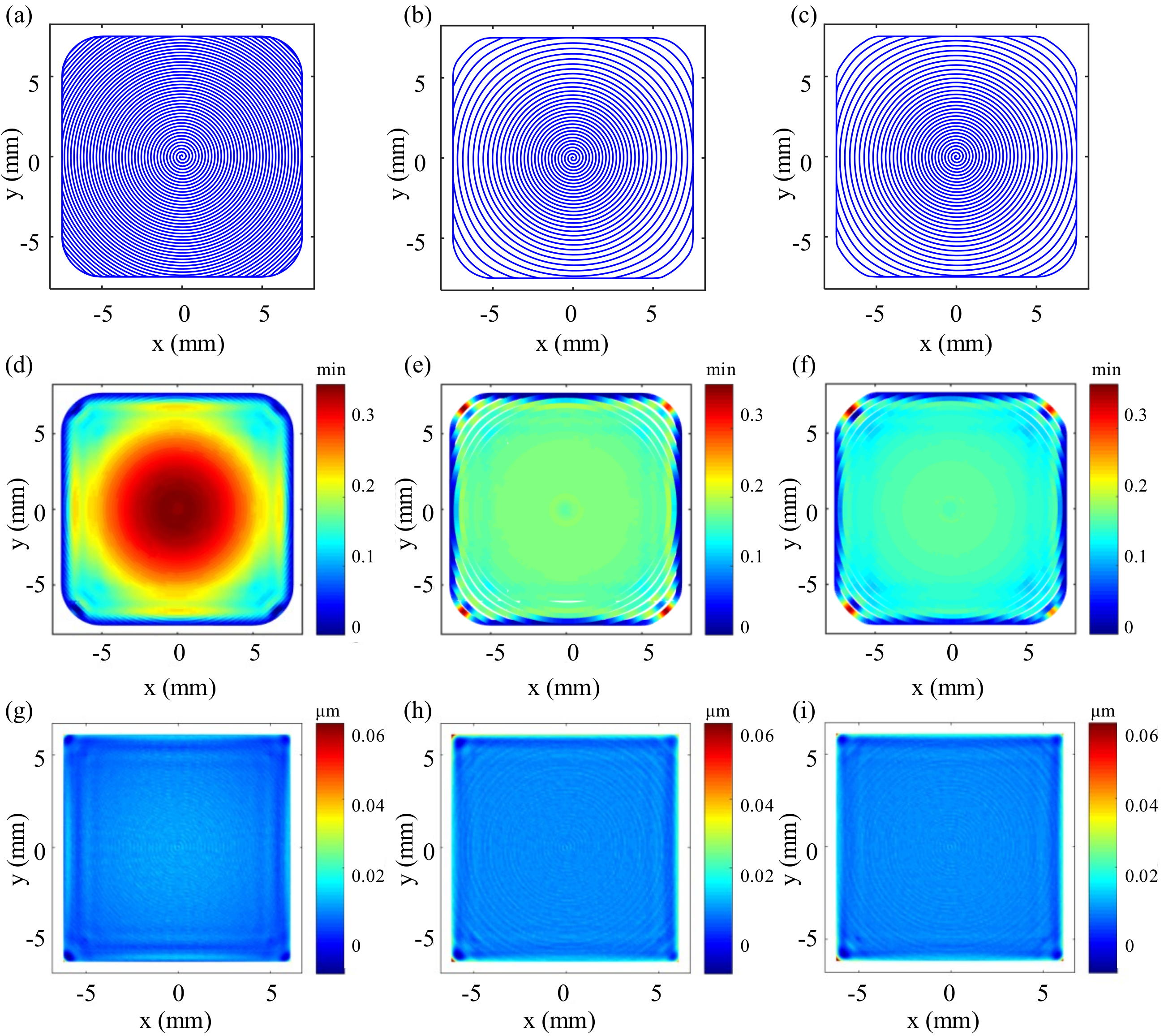
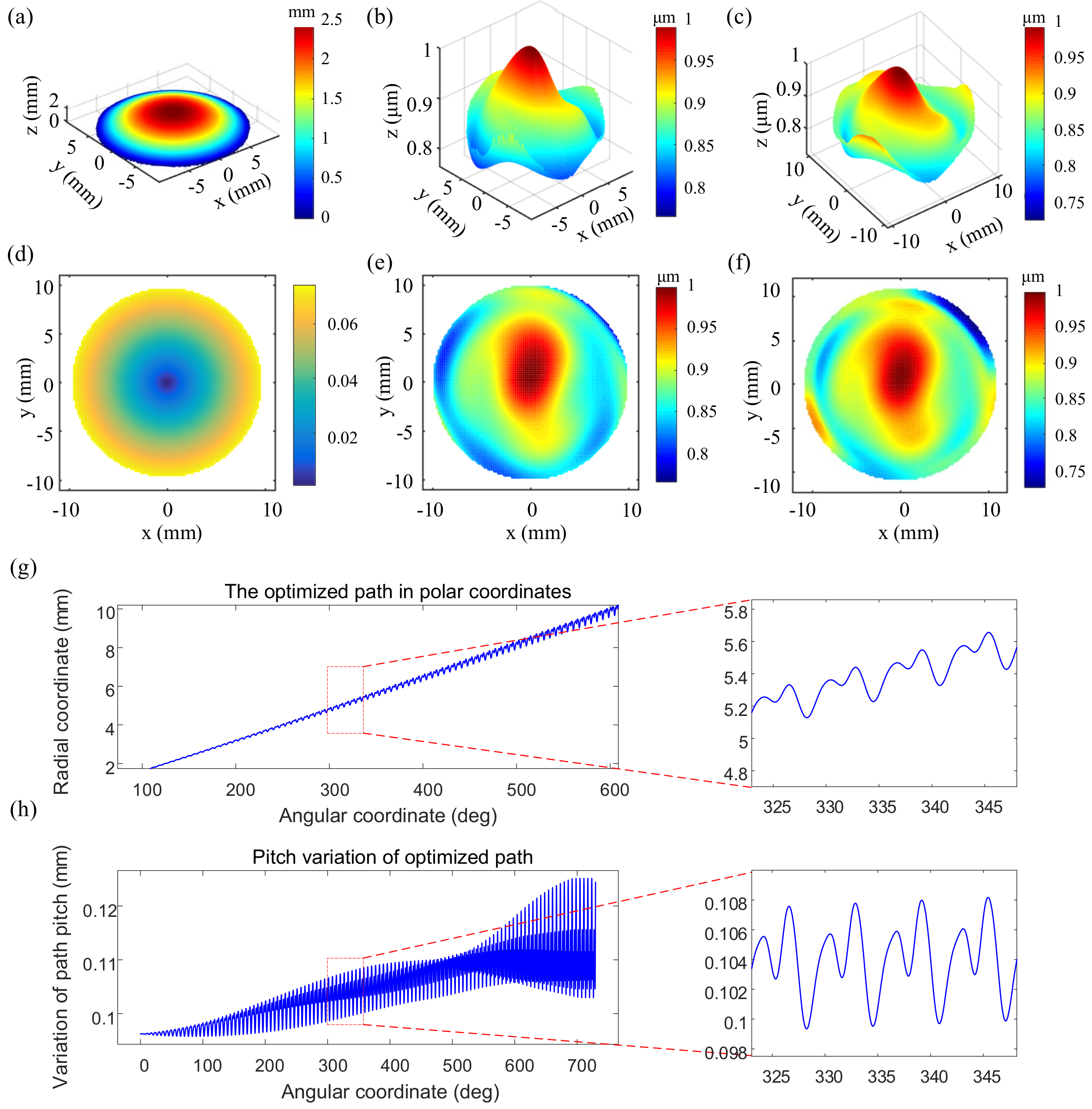
4.3. Variable Pitch Spiral Path Planning Method

In order to realize the optimization process of the spiral polishing path efficiently and quickly, this paper proposes to plan the variable pitch spiral polishing path on a two-dimensional plane. Moreover, the path pitch along the radial direction of the spiral path is iteratively optimized according to the proposed path spacing optimization model in Section 4.2. At the same time, when the variable pitch 2D path is projected onto a 3D target surface, in order to avoid as much as possible the impact of slope change on the pitch of the projected path, a path spacing compensation factor based on the gradient change distribution of the target surface is introduced. After several iterative optimizations, the final variable pitch spiral-polishing path with seamless transition will be obtained. Figure 7a gives the complete planning flowchart for the optimized path with variable pitch.

Although practical fluid jet polishing is hardly affected by the polishing edge effect [21], the edge-up phenomenon occurs when performing polishing removal simulations, which is a common problem that is difficult to avoid when solving the dwell time [22,23]. In this algorithm, to avoid the influence of this phenomenon on the solution in the region of interest, the polished surface and its form error will extend outward by a specified distance, and so does the planned polishing path, as shown in Figure 7b. Through several simulation experiments, it was found that when the extension distance is specified as $1.5R_{tif}$, the influence of the edge-up phenomenon on the region of interest can be effectively avoided and a better removal effect obtained.

In this algorithm, we first determine the range of path spacing changes according to Equation (7) and give the corresponding path optimization model specified by Equations (5) or (6). Then, the initial planned Archimedes spiral path can be given by Equation (8) as follows:

$$\left\{\begin{array}{c}{r}_0=0.075R_{tif};p_0=P_{min};{\theta }_m=m\Delta \theta ,m=0,\dots ,M\hfill \\ M=\mathrm{INT}\left(\frac{2\pi R_{max}}{\Delta \theta P_0}\right);r_m=r_0+p_0\times \frac{{\theta }_m}{2\pi }\hfill \end{array}\right.$$

(8)

where ${\gamma }_0$ represents the starting spiral radius; $p_0$ represents the pitch of the Archimedean spiral path; $\Delta \theta$ represents the angular coordinate increment of adjacent path points in the initial planned path; $R_{\max }$ represents the limit of the radius of the circular area of the initial planned Archimedes spiral path; INT represents the operation of rounding down. For a rectangular workpiece and a circular workpiece, Equation (9) gives the calculation method of $R_{\max }$ in two cases. The initial Archimedes spiral path bounded by the maximum radius calculated by Equation (9) can ensure fast convergence of the iterative optimization process. ${\theta }_m$, $r_m$ represent the angular coordinate and radial coordinate of the m-th path point of the initially planned path in polar coordinates, respectively.

$$\left\{\begin{array}{c}{R}_{max}=\sqrt{{\left(\frac{L_x+3R_{tif}}{2}\right)}^2+{\left(\frac{L_y+3R_{tif}}{2}\right)}^2},\mathrm{for}\mathrm{rectangular}\mathrm{shape}\hfill \\ R_{max}=\frac{2R+3R_{tif}}{2},\mathrm{for}\mathrm{circular}\mathrm{shape}\hfill \end{array}\right.$$

(9)

in which $L_x$, $L_y$ represent the length and width of the original rectangular workpiece, respectively, and R represents the radius of the original circular workpiece.

The algorithm extracts the boundary curve of the projection of the target surface on the $xoy$ plane, and the new curve obtained by offsetting the distance of $1.5R_{tif}$ outward is used as the constraint boundary of the subsequent path planning. Assume that the boundary can be expressed in polar coordinates as $r_b=Boundary\left({\theta }_b\right),0\le {\theta }_b\le 2\pi$, then the radial coordinates of all the path points beyond the constraint boundary are set as the radial coordinates of the corresponding boundary points, and the angular coordinates remain unchanged. Then, Equation (10) can be used to calculate the constrained path.

$$r_b=Boundary\left(mod\left(\theta ,2\pi \right)\right);r=r_b,r\ge r_b$$

(10)

We need to extend the target surface and calculate the slope distribution surface corresponding to the extended surface. Then, according to Equation (11), the path points are transformed from the polar coordinate system to the Cartesian coordinate system and are projected onto the calculated slope distribution surface and the extended form error surface, respectively. The z coordinate of each projection point obtained by projecting on the slope distribution surface and the form error surface respectively correspond to the slope $k_{slope}$ and the form error $z_h$. According to Equation (12), we can calculate the change of path spacing after one iterative optimization.

$$\left\{\begin{array}{c}x=x_0+rcos\theta ;y=y_0+rsin\theta \hfill \\ z_h=\Gamma (error\_ext,x,y);k_{slope}=\Gamma (targetslopesurf\_ext,x,y)\hfill \end{array}\right.$$

(11)

in which $\Gamma (error\_ext,x,y)$ and $\Gamma (targetslopesurf\_ext,x,y)$ represent projection operations on the extended form error surface $error\_ext$ and the slope distribution surface $targetslopesurf\_ext$ corresponding to the extended target surface, respectively.

$$p=\left\{\begin{array}{c}{p}_{rms}\left(z_h\right)/\phantom{p_{rms}\left(z_h\right)\sqrt{{k^2}_{slope}+1}}\sqrt{{k^2}_{slope}+1},\mathrm{RMS}-\mathrm{based}\mathrm{optimization}\hfill \\ p_{pv}\left(z_h\right)/\phantom{p_{pv}\left(z_h\right)\sqrt{{k^2}_{slope}+1}}\sqrt{{k^2}_{slope}+1},\mathrm{PV}-\mathrm{based}\mathrm{optimization}\hfill \end{array}\right.$$

(12)

Finally, an unconstrained variable pitch spiral path after one iterative optimization is obtained according to Equation (13). Then, using Equation (10) to calculate the variable pitch spiral path with boundary constraints and eliminate the repeated path with the edge at the end of the path, a variable pitch spiral path with boundary constraints after one iteration optimization is obtained. After the iterative optimization is converged, the final variable pitch path is derived by resampling $\Delta \theta$ making point-to-point distance constant along the path.

$$\left\{\begin{array}{c}N=\mathrm{INT}\left(2\pi /\phantom{2\pi \Delta \theta }\Delta \theta \right)\hfill \\ {\theta }_k=k\Delta \theta ;r_k=r_0+\frac{p_1{\theta }_k}{2\pi },0\le k\le N\hfill \\ {\theta }_k={\theta }_{k-N}+2\pi ;r_k=r_{k-N}+p_{k-N},k>N\hfill \end{array}\right.$$

(13)

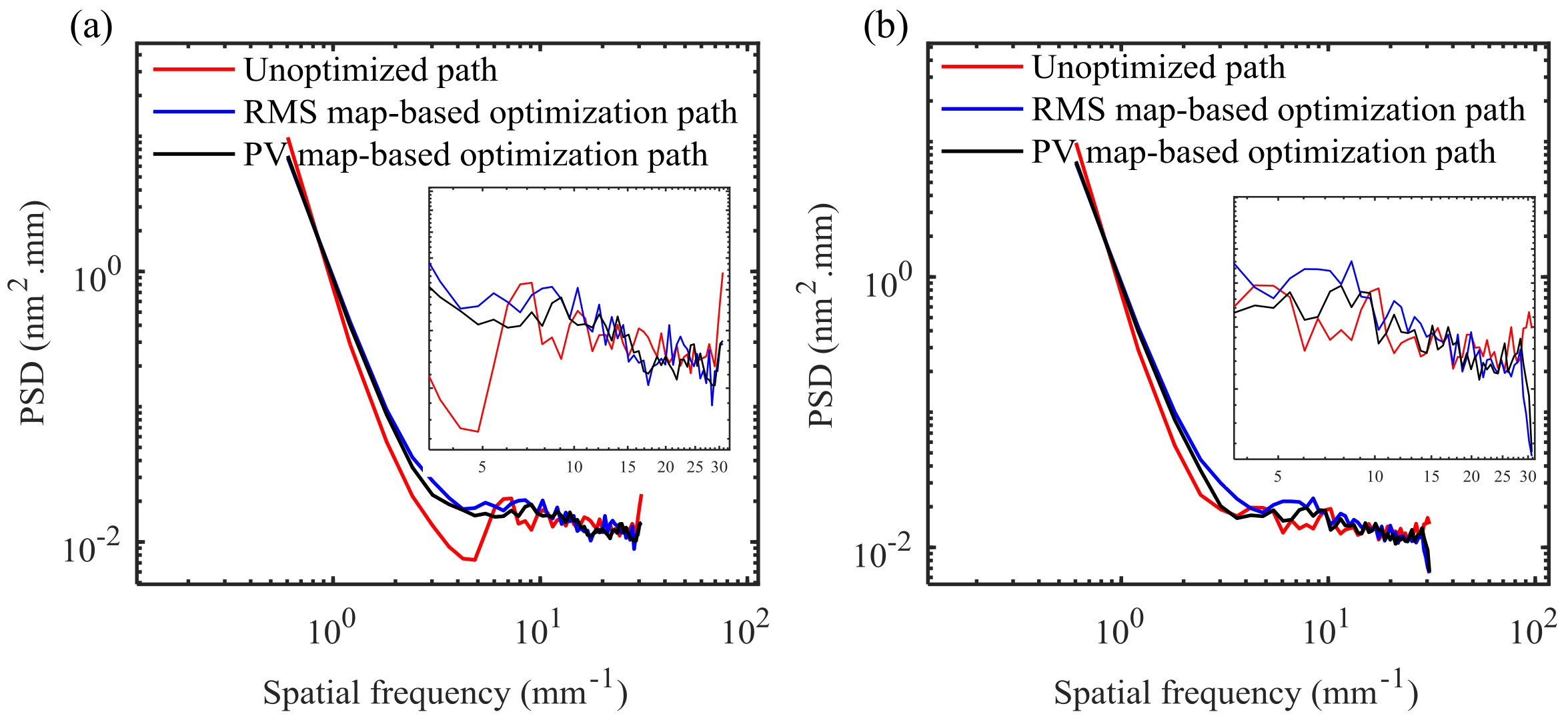
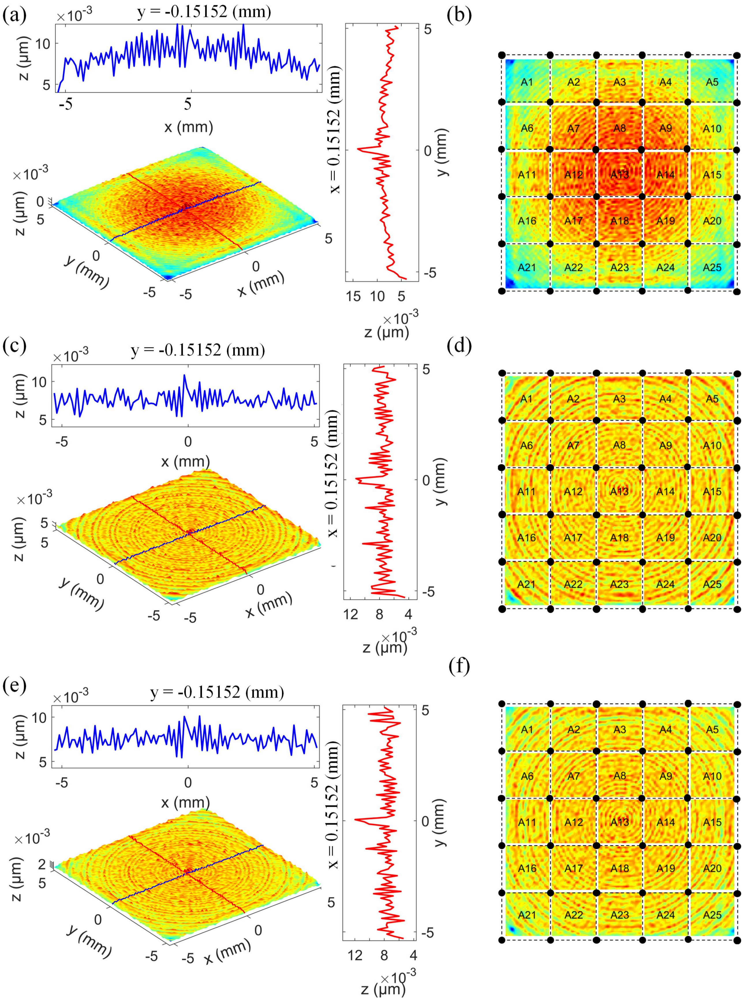
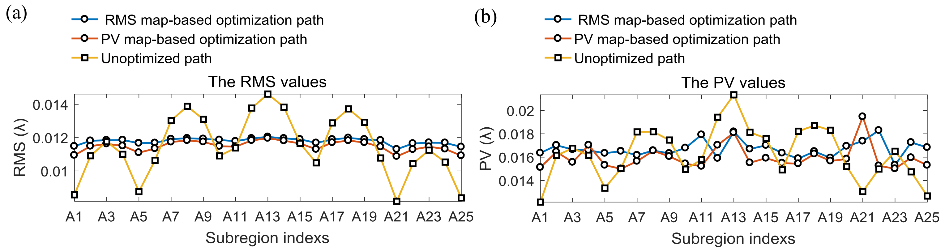
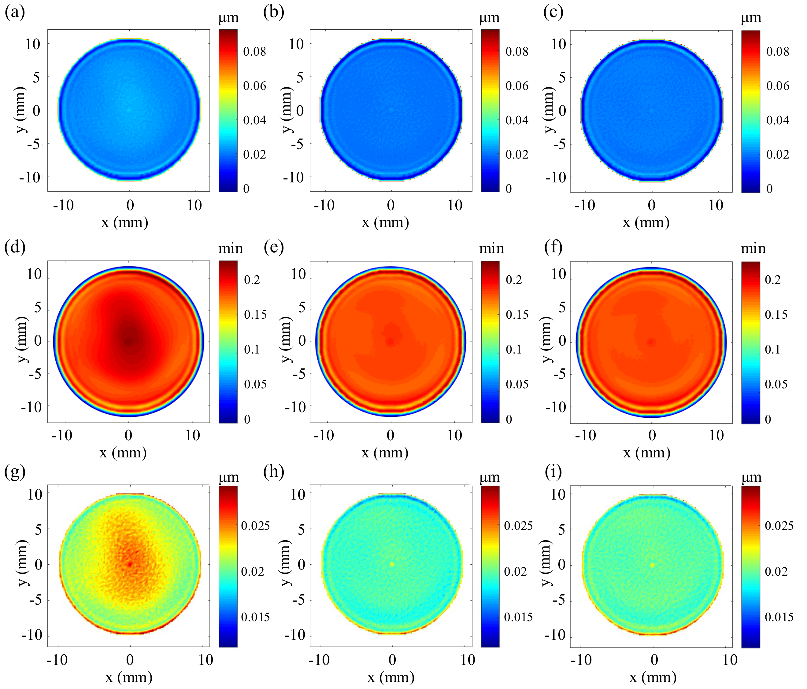
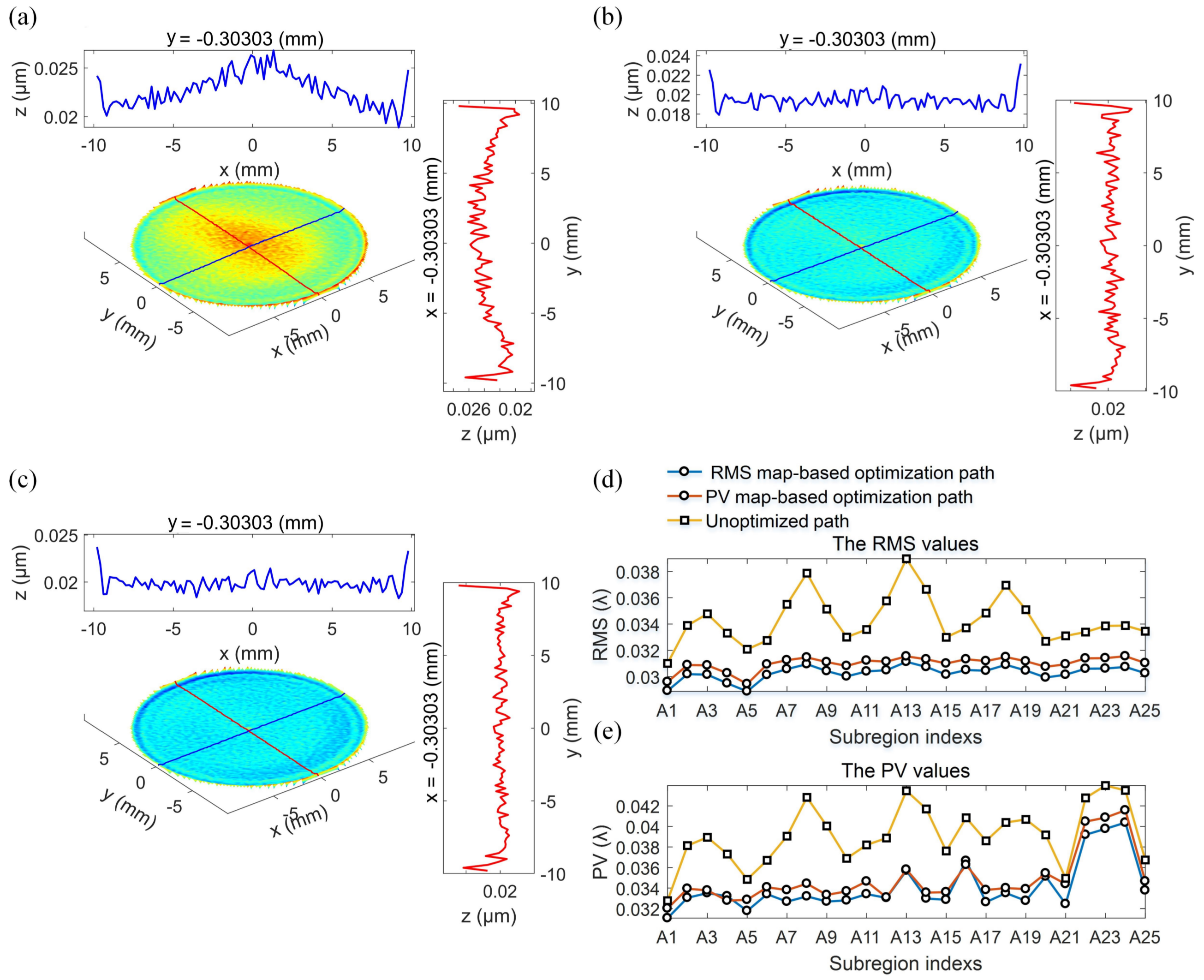
5. Comparative Study of Optimization Strategies

In order to verify the validity and feasibility of the proposed residual error optimization strategy based on the distribution of surface form error, the comparative correction polishing studies were performed in this section for one planar test piece and one aspherical test piece. The comparison results of the residual error distribution before and after optimization both verify the validity and feasibility of the proposed strategy.

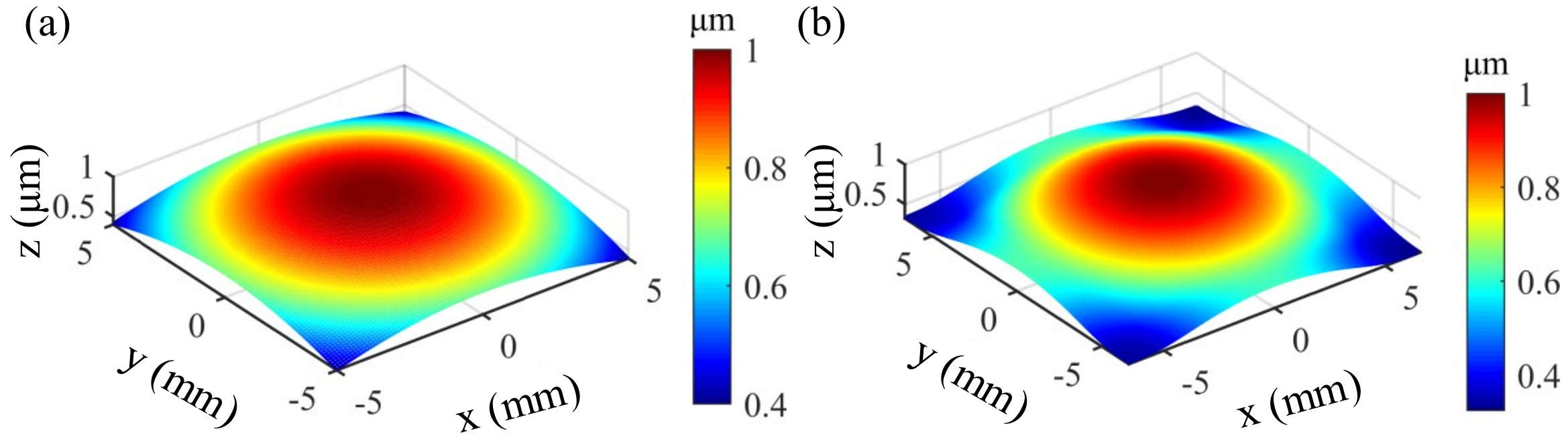
5.1. Case 1: Planar Workpiece

In this case, a planar test piece with a length of 10 mm and width of 10 mm is again selected. Figure 8 shows the initial typical form error distribution and the extended form error distribution, respectively. It can be seen that the distribution of form error is a typical convex surface form with a height variation range of $0.5\mathsf{\mu }$m to $1\mathsf{\mu }$m. The TIF specified in Section 3 is again used in this simulation. Therefore, we can directly use the RMS-map-based (Equation (5)) and PV-map-based path-pitch model (Equation (6)) obtained in Section 3 to optimize the initially planned polishing paths. In addition, since it is a planar specimen, the slope compensation factor in Equation (11) is null, i.e., $k_{slope}=0$.

Table 3. Parameters for planning the initial spiral-polishing path.

$p_{\min }$ (mm)	$p_{\max }$ (mm)	$p_0$ (mm)	$\Delta \theta$ (deg)	$r_0$ (mm)
0.2	0.6	0.2	$\pi$/6	0.01

shows the key parameters for planning the spiral-polishing path with optimized variable pitch.

According to the kind of optimization model, we get three kinds of polishing paths, namely the unoptimized path, RMS-map-based optimized path and PV-map-based optimized path. Figure 9a shows the initially planned spiral-polishing path with boundary constraints. Using the two proposed optimization models respectively to optimize the initial path given in Figure 9a, the corresponding optimized path distributions are obtained, as shown in Figure 9b,c. It can be seen that the polishing path pitch before optimization is always 0.2 mm and is evenly distributed. Although there are subtle differences in paths optimized by different optimization models, their path pitches are continuously changed with the variation of the surface form error in the range of 0.2 mm to 0.6 mm.

By solving the dwell times corresponding to the three polishing paths, the dwell time distribution maps corresponding to the three polishing paths are obtained, as shown in Figure 9d–f. It can be seen from Figure 9d that the dwell time distribution corresponding to the initial equally-spaced spiral polishing path is consistent with the initial form error distribution. It further verifies the experimental results obtained in Section 3.2.2, that is, when the path spacing is constant, there is a positive linear relationship between the dwell time of each dwell point and the amount of form error. For the optimized paths, especially in the regions we care about, the dwell time of each dwell point does not change very much. From Figure 3b in Section 3.2.1, it can be seen that there is also a positive linear relationship between the path spacing within a certain range (0.2 mm–0.6 mm) and the dwell time of each point when bulk material removal depth is constant. It is under the combined influence of bulk material removal depth and path spacing that the dwell time at each point on the optimized path remains mostly the same. To some extent, the optimized path is a good way to improve dwell time distribution. Since spacing of the planned dwell points along the path is basically the same, the optimized polishing path will run under a more stable polishing speed, which is crucial for obtaining a stable polishing process [24]. Figure 9g–i respectively shows the residual error distribution obtained by figuring the extended form error using the three polishing paths, respectively. It can be seen that the strategy of extending the path and the surface form error effectively prevents material removal of the region of interest from being affected by the edge-warping phenomenon. Compared to the residual error distribution before optimization, the imprint of the initial surface form the error distribution can hardly be found visually in the optimized residual error distributions.

As shown in Figure 10a,c,e, in order to further clearly compare and quantify the difference of the residual error distribution before and after optimization and the effects of two optimization models on the residual error distribution, the residual error distribution of the region of interest is extracted. At the same time, two cross-sectional profiles passing through the center origin and parallel to the x-axis and y-axis are respectively given for each residual error distribution. From Figure 10a, it can be seen that the residual error distribution corresponding to the unoptimized polishing path is highly similar to the distribution of the parent surface form error shown in Figure 8a, that is the error shows a decreasing trend from the center to the periphery. However, the residual error distribution after optimization shown in Figure 10c,e, respectively, is more flattened and is almost unaffected by the distribution of parent form error.

Considering the use of RMS and PV values of the overall residual error to evaluate the residual error distribution, there are two disadvantages: (i) the optimization effect of the proposed residual error optimization strategy on residual error distribution cannot be evaluated intuitively and comprehensively; (ii) it is difficult to compare subtle differences in the residual error distribution obtained by the two optimization models proposed. In this paper, a method of sub-domain evaluation is proposed. Firstly, the residual error of the region of interest is evenly divided into 25 sub-regions, as shown in the Figure 10b,d,f. Then, the RMS and PV values of the residual error corresponding to each sub-region are calculated, and the corresponding RMS and PV curves are plotted. Figure 11a,b shows the RMS and PV curves obtained from the simulation results, respectively. It can be seen that, using the sub-domain evaluation method, the RMS curves obtained by the three polishing paths all show both obvious and inconspicuous peaks, and the occurrence frequency of the peaks has a certain regularity. The curve peaks appear in the ranges A1–A5, A6–A10, A11–A15, A16–A20 and A21–A25, respectively. For the range A1–A5, if the average value of the form errors corresponding to each sub-area is plotted as a curve, a similar peak curve is obtained. From the results obtained in Section 3, we know that the RMS value of the residual error increases with the material removal depth; therefore, the resulting RMS curve also exhibits the peak. This can also explain the formation of the corresponding peak in other ranges. In addition, the average amplitude and corresponding amplitude fluctuation range of the RMS curve with optimization are both smaller than that without optimization. This is because adjustment of the path spacing effectively compensates for the influence of different material removal depths caused by the surface form error distribution on the residual error, which greatly reduces the influence of the distribution of parent surface form error on the child residual error distribution.

There are multiple outlier points on the PV curve given in Figure 11b, which appear at the positions of A1, A5, A13, A21 and A25, respectively. Comparing the residual error distribution shown in Figure 10, we can see that these outlier points appear at the center of the residual error region and at the four edge corners, respectively. The reason for the abrupt change of PV value in the residual error region corresponding to A13 is related to the center effect produced by the spiral path polishing. The sudden change in PV value at the four edge corners may be related to a 90 degree change in the polishing direction of the planned polishing path at the four corner points. Regardless of the above outlier points, it can be seen that the residual errors obtained by using the PV-map-based optimization model have smaller and closer PV values. In addition, it can be seen that the RMS-map-based optimization model improves the spread of PV values over the sub-regions of residual error.

As shown in Figure 6b,d, the ideal RMS and PV values for the two optimized models are RMS = 0.0097342 $\lambda$ and PV = 0.013193 $\lambda$, respectively. However, we found that RMS and PV values obtained after optimization are about 20% larger than the target values. This may be related to the fact that the bulk material removal depth varies in the adjacent path interval caused by varying surface form error, unlike the constant bulk material removal depth in the experiment in Section 3.

Power spectral density analysis was performed on the residual errors obtained by the above three polishing paths, and the results along the x-direction and y-direction are, respectively, shown in Figure 12a,b. It can be seen from the PSD curves that whether the path optimization model is based on the RMS or PV map, the amplitude variation of the power spectral density of the mid-spatial frequency components in the residual error obtained by the optimized path is more stable. It can be concluded that the proposed optimization strategy can effectively smooth the distribution of MSF error components in the residual error.

5.2. Case 2: Aspheric Workpiece

To further verify the feasibility of the proposed optimization strategy for corrective polishing of complex surfaces, in this case, we selected the aspherical surface shown in Figure 13a as the test sample.

Table 4. Detailed parameters of the aspheric surface.

$R_0$ (mm)	c (mm${}^{-1}$)	D (mm)	k	$a_2$	$a_3$	$a_4$
20	$1/R_0$	20	−0.32	−1.5 × 10${}^{-14}$	−1.5 × 10${}^{-14}$	−3.0 × 10${}^{-16}$

gives the specific parameters of the aspheric surface, which is expressed by Equation (14) as follows:

$$z=\frac{c\left(x^2+y^2\right)}{1+\sqrt{1-c^2\left(1+k\right)\left(x^2+y^2\right)}}+a_2{\left(x^2+y^2\right)}^2+a_3{\left(x^2+y^2\right)}^3+a_4{\left(x^2+y^2\right)}^4+\cdots$$

(14)

where $R_0$ represents the radius of curvature of the aspherical vertex; c represents the curvature of the aspherical vertex, with $c=1/R_0$; D represents the aspherical aperture; k represents the quadratic constant; $a_2$, $a_3$, $a_4$ represent the coefficients of higher order terms in the aspheric equation, respectively.

Figure 13d shows the slope distribution corresponding to the aspherical surface. It can be seen that the slope of the surface is rotationally symmetric and gradually increases from the center to the periphery. Figure 13b,c,e,f respectively shows the isometric and top view of the aspherical surface form error and of the extended surface form error obtained after extending a distance of $1.5R_{tif}$. Since the material removal depth variation in all regions in this case is small (about 0.75 $\mathsf{\mu }$m to 1 $\mathsf{\mu }$m), the chosen minimum path in Equation (7) and its variation range are narrow. The path obtained in the Cartesian space is too dense to observe the effect of pitch change by the naked eye; thus, Figure 13g,h gives the RMS-map-based optimization path in polar coordinate and its pitch-variation along the path.

Similar to Case 1, Figure 14 shows the distribution of residual error and dwell time, respectively. It can be seen that the residual error distribution obtained by the optimization strategy is hardly affected by the distribution of parent form error, and the approximately uniform distribution of dwell time indicates that the polishing speed for the whole process is maintained at a stable level, such that polishing dynamics are optimized. Figure 15a–c shows the profile changes of the two section lines corresponding to three residual errors, respectively. The imprint of the parent form error is almost invisible in the optimized section profile curve, which further verifies the usefulness of the proposed optimization strategy. For the circular workpiece, the sub-domain evaluation strategy proposed in Section 5.1 is also used to obtain the RMS and the PV curves in sub-regions of the residual error, as shown in Figure 15d,e. It can be seen from the variation of the curve that the optimization strategy can significantly improve the spread of RMS and PV values across the residual error and that different optimization models result in different optimization effects. It can be concluded that for the corrective polishing of the surface, the proposed optimization strategies are both effective, and the distribution of residual error is significantly improved.

6. Conclusions

This paper deeply studied and analyzed the influence law of bulk material removal depth and path spacing on residual error. It was found that with the increase in surface form error, the RMS and PV values of the residual error also increase. For deterministic polishing, a reasonable polishing path spacing should be less than 3/10 of the diameter of the TIF. In this range, as the path spacing increases, the corresponding RMS and PV values of the residual error increase linearly, and the larger the bulk material removal depth, the greater the influence of the path spacing on the residual error. This paper further proposed a residual error optimization strategy based on surface form error distribution. In this strategy, the mapping relationship between bulk material removal depth, path spacing and residual error was established and integrated into the optimization goal. The influence of varying bulk material removal depths resulting from the form error distribution on the residual error was compensated by adjusting the path spacing, and a specific path optimization model was obtained. In the implementation of this process, a variable-pitch polishing path is planned in accordance with the path optimization model and the actual surface form error distribution of the workpiece to be polished. Polishing with this optimized path can effectively optimize the residual error distribution and greatly reduce the influence of parent form error distribution on outcome RMS and PV values in sub-regions of the residual error. Furthermore, this optimization drastically reduces variations in tool feed across the workpiece, which facilitates dynamic control of the process.

References

1. Guo, Z.; Jin, T.; Ping, L.; Lu, A.; Qu, M. Analysis on a deformed removal profile in FJP under high removal rates to achieve deterministic form figuring. Precis. Eng. J. Int. Soc. Precis. Eng. Nanotechnol. 2018, 51, 160–168. [Google Scholar] [CrossRef]
2. Brinksmeier, E.; Mutlugünes, Y.; Klocke, F.; Aurich, J.C.; Shore, P.; Ohmori, H. Ultra-precision grinding. CIRP Ann. 2010, 59, 652–671. [Google Scholar] [CrossRef]
3. Zhang, L.; Han, Y.J.; Fan, C.; Tang, Y.; Song, X.P. Polishing path planning for physically uniform overlap of polishing ribbons on free form surface. Int. J. Adv. Manuf. Technol. 2017, 92, 4525–4541. [Google Scholar] [CrossRef]
4. Jones, R.A. Optimization of computer controlled polishing. Appl. Opt. 1977, 16, 218–224. [Google Scholar] [CrossRef] [PubMed]
5. Wan, S.L.; Zhang, X.C.; Zhang, H.; Xu, M.; Jiang, X.Q. Modeling and analysis of sub-aperture tool influence functions for polishing curved surfaces. Precis. Eng. J. Int. Soc. Precis. Eng. Nanotechnol. 2018, 51, 415–425. [Google Scholar] [CrossRef]
6. Cao, Z.C.; Cheung, C.F.; Liu, M.Y. Model-based self-optimization method for form correction in the computer controlled bonnet polishing of optical free form surfaces. Opt. Express 2018, 26, 2065–2078. [Google Scholar] [CrossRef] [PubMed]
7. Beaucamp, A.; Namba, Y. Super-smooth finishing of diamond turned hard X-ray molding dies by combined fluid jet and bonnet polishing. CIRP Ann. Manuf. Technol. 2013, 62, 315–318. [Google Scholar] [CrossRef]
8. Temple, P.A.; Lowdermilk, W.H.; Milam, D. Carbon dioxide laser polishing of fused silica surfaces for increased laser-damage resistance at 1064 nm. Appl. Opt. 1982, 21, 3249–3255. [Google Scholar] [CrossRef] [PubMed]
9. Ghadikolaei, A.D.; Vahdati, M. Experimental study on the effect of finishing parameters on surface roughness in magneto-rheological abrasive flow finishing process. Proc. Inst. Mech. Eng. Part B. J. Eng. Manuf. 2014, 229, 1517–1524. [Google Scholar] [CrossRef]
10. Stognij, A.I.; Novitskii, N.N.; Stukalov, O.M. Nanoscale ion beam polishing of optical materials. Tech. Phys. Lett. 2002, 28, 17–20. [Google Scholar] [CrossRef]
11. Li, W.; Bin, F.; Shi, C.; Jia, W.; Bin, Z. A path planning method used in fluid jet polishing eliminating lightweight mirror imprinting effect. Proc. SPIE 2014, 9281. [Google Scholar] [CrossRef]
12. Wang, T.; Cheng, H.; Zhang, W.; Yang, H.; Wu, W. Restraint of path effect on optical surface in magnetorheological jet polishing. Appl. Opt. 2016, 55, 935–942. [Google Scholar] [CrossRef] [PubMed]
13. Dunn, C.; Walker, D. Pseudo-random tool paths for CNC sub-aperture polishing and other applications. Opt. Express 2008, 16, 18942–18949. [Google Scholar] [CrossRef] [PubMed]
14. Wang, C.; Wang, Z.; Xu, Q. Unicursal random maze tool path for computer-controlled optical surfacing. Appl. Opt. 2015, 54, 10128–10136. [Google Scholar] [CrossRef] [PubMed]
15. Takizawa, K.; Beaucamp, A. Comparison of tool feed influence in CNC polishing between a novel circular-random path and other pseudo-random paths. Opt. Express 2017, 25, 22411–22424. [Google Scholar] [CrossRef] [PubMed]
16. Wang, C.; Yang, W.; Ye, S.; Wang, Z.; Yang, P.; Peng, Y.; Guo, Y.; Xu, Q. Restraint of tool path ripple based on the optimization of tool step size for sub-aperture deterministic polishing. Int. J. Adv. Manuf. Technol. 2014, 75, 1431–1438. [Google Scholar] [CrossRef]
17. Hou, J.; Liao, D.; Wang, H. Development of multi-pitch tool path in computer-controlled optical surfacing processes. J. Eur. Opt. Soc.-Rapid Publ. 2017, 13, 22. [Google Scholar] [CrossRef]
18. Hu, H.; Dai, Y.; Peng, X. Restraint of tool path ripple based on surface error distribution and process parameters in deterministic finishing. Opt. Express 2010, 18, 22973–22981. [Google Scholar] [CrossRef] [PubMed]
19. Dong, Z.; Cheng, H. Toward the complete practicability for the linear-equation dwell time model in subaperture polishing. Appl. Opt. 2015, 54, 8884–8890. [Google Scholar] [CrossRef] [PubMed]
20. Dong, Z.; Cheng, H.; Tam, H.Y. Robust linear equation dwell time model compatible with large scale discrete surface error matrix. Appl. Opt. 2015, 54, 2747–2756. [Google Scholar] [CrossRef] [PubMed]
21. Guo, P.; Fang, H.; Yu, J. Edge effect in fluid jet polishing. Appl. Opt. 2006, 45, 6729–6735. [Google Scholar] [CrossRef] [PubMed]
22. Li, H.; Zhang, W.; Yu, G. Study of weighted space deconvolution algorithm in computer controlled optical surfacing formation. Chin. Opt. Lett. 2009, 7, 627–631. [Google Scholar] [CrossRef]
23. Wang, C.; Yang, W.; Wang, Z.; Yang, X.; Hu, C.; Zhong, B.; Guo, Y.; Xu, Q. Dwell-time algorithm for polishing large optics. Appl. Opt. 2014, 53, 4752–4760. [Google Scholar] [CrossRef] [PubMed]
24. Guillerna, A.B.; Axinte, D.; Billingham, J. The linear inverse problem in energy beam processing with an application to abrasive waterjet machining. Int. J. Mach. Tools Manuf. 2015, 99, 34–42. [Google Scholar] [CrossRef]
Figure 1. (a) Tool influence function (TIF) with Gaussian shape; (b) tool path design.
Applsci 08 01814 g001
Figure 2. Effect of path pitch on (a) residual error and (b) other path parameters (bulk material removal depth = 0.5 μ m).
Applsci 08 01814 g002
Figure 3. (a) y-direction power spectral density (PSD) results for different path pitches; (b) influence of the bulk material removal depth on residual error (path pitch = 0.2 mm); (c) y-direction PSD results for different path pitches and bulk material removal depths.
Applsci 08 01814 g003
Figure 4. The influence of path spacing variations on the (a,c) root-mean-square (RMS) and (b,d) peak-to-valley (PV) of the residual error resulting from different bulk material removal depths.
Applsci 08 01814 g004
Figure 5. (a) Original RMS map; (b) fitted map of RMS; (c) original PV map; (d) fitted map of PV.
Applsci 08 01814 g005
Figure 6. (a) RMS contours of the residual error; (b) relationship curve between bulk material removal depth and the path pitch based on the RMS map; (c) PV contours of the residual error; (d) relationship curve between bulk material removal depth and the path pitch based on the PV map.
Applsci 08 01814 g006
Figure 7. (a) The generation flowchart of the optimized path with variable pitch; (b) control strategy for edge-warping effect.
Applsci 08 01814 g007
Figure 8. (a) Original form error distribution; (b) extended form error distribution.
Applsci 08 01814 g008
Figure 9. (a) Boundary-defined unoptimized path with constant pitch; (b) RMS-map-based optimized path with varying pitch; (c) PV-map-based optimized path with varying pitch; (d) dwell time map along the unoptimized path; (e) dwell time map along the RMS-map-based optimized path; (f) dwell time map along the PV-map-based optimized path; (g) residual error corresponding to the unoptimized path; (h) residual error corresponding to the RMS-map-based optimized path; (i) residual error corresponding to the PV-map-based optimized path.
Applsci 08 01814 g009
Figure 10. Residual error of the concerned surface region polished along: (a,b) the unoptimized path; (c,d) the RMS-map-based optimized path; and (e,f) the PV-map-based optimized path.
Applsci 08 01814 g010
Figure 11. (a) RMS and (b) PV curves for sub-regional evaluation.
Applsci 08 01814 g011
Figure 12. PSD analysis results of residual error in the (a) x-direction and (b) y-direction.
Applsci 08 01814 g012
Figure 13. (a) Aspheric surface; (b) isometric view of the original form error distribution; (c) isometric view of the extended form error distribution; (d) slope distribution of the aspheric surface; (e) top view of the original form error distribution; (f) top view of the extended form error distribution; (g) RMS-map optimization path in polar coordinates; (h) variation of path pitches of the RMS-map optimization path.
Applsci 08 01814 g013
Figure 14. Residual error corresponding to: (a) the unoptimized path; (b) the RMS-map-based optimized path; and (c) the PV-map-based optimized path. Dwell time map along: (d) the unoptimized path; (e) the RMS-map-based optimized path; and (f) the PV-map-based optimized path. Residual error of the concerned surface region polishing along: (g) the unoptimized path; (h) the RMS-map-based optimized path; and the (i) PV-map-based optimized path.
Applsci 08 01814 g014
Figure 15. Residual error of the concerned surface region polished along: (a) the unoptimized path; (b) the RMS-map-based optimized path; and (c) the PV-map-based optimized path; (d) RMS and (e) PV curves for sub-regional evaluation.
Applsci 08 01814 g015