Article

Solution Strategies for Linear Inverse Problems in Spatial Audio Signal Processing

1
Department of Power Mechanical Engineering, National Tsing Hua University, No. 101, Section 2, Kuang-Fu Road, Hsinchu 30013, Taiwan
2
Department of Electrical Engineering, National Chiao Tung University, No. 1001, Ta-Hsueh Road, Hsinchu 30013, Taiwan
*
Author to whom correspondence should be addressed.
Appl. Sci. 2017, 7(6), 582; https://doi.org/10.3390/app7060582
Submission received: 30 March 2017 / Revised: 15 May 2017 / Accepted: 26 May 2017 / Published: 5 June 2017
(This article belongs to the Special Issue Spatial Audio)

Abstract

:
The aim of this study was to compare algorithms for solving inverse problems generally encountered in spatial audio signal processing. Tikhonov regularization is typically utilized to solve overdetermined linear systems in which the regularization parameter is selected by the golden section search (GSS) algorithm. For underdetermined problems with sparse solutions, several iterative compressive sampling (CS) methods are suggested as alternatives to traditional convex optimization (CVX) methods that are computationally expensive. The focal underdetermined system solver (FOCUSS), the steepest descent (SD) method, Newton’s (NT) method, and the conjugate gradient (CG) method were developed to solve CS problems more efficiently in this study. These algorithms were compared in terms of problems, including source localization and separation, noise source identification, and analysis and synthesis of sound fields, by using a uniform linear array (ULA), a uniform circular array (UCA), and a random array. The derived results are discussed herein and guidelines for the application of these algorithms are summarized.

Graphical Abstract

1. Introduction

Numerous inverse problems exist in the field of acoustics. For example, nearfield acoustic holography (NAH) is a noise source identification method that reconstructs a surface field of the source on the basis of sound pressure measured in the nearfield of the source [1,2,3,4,5]. The deconvolution approach for the mapping of acoustic sources (DAMAS) is also a method for noise source identification [6]. Another example is the source signal separation problem, where an individual source signal is to be extracted from a mixed array of signals [7]. Inverse problems can also be found in source sound field synthesis (SFS) problems, where the sound field produced by secondary sources is to be matched with a target field [8,9]. Other examples include sound field control [10,11], crosstalk cancellation in binaural audio rendering [12], noise reduction in speech enhancement [13], room response equalization, and dereverberation [14,15]. In linear range acoustics, each of these problems can be formulated as a linear system (Ax = b). The current study focused on the solutions of farfield noise source identification problems, sound source localization and separation problems, and sound field analysis (SFA) and synthesis (SFS) problems. Although inverse solutions of acoustic problems have long been investigated by researchers, according to our review of the literature, no conclusive results that give solution strategies and parameter choice guidelines can be found in the literature. Furthermore, although audio quality is the chief concern in practical audio reproduction, most previous research has examined general numerical accuracy and stability. This study explored these problems from the perspective of reproduced signal quality. Solution strategies were compared in a unified framework, and guidelines of parameter choice are summarized herein.
In general, inverse problems can be divided into two categories: overdetermined and square systems, and underdetermined systems. To solve overdetermined systems, least-squares methods, Tikhonov regularization (TIKR) [16], and truncated singular value decomposition (TSVD) are commonly used. Traditionally, Morozov’s discrepancy principle, generalized cross-validation (GCV), and the L-curve method can be used to choose the regularization parameter in the TIKR method [17,18,19,20]. However, solution methods that are better suited to audio applications than conventional approaches are proposed in this work. In particular, golden section search (GSS) [21] is applied to find optimal regularization parameters. To solve underdetermined problems, compressive sampling (CS) [22,23] solved by using convex optimization (CVX) [24,25,26] is a widely used approach that is known to be computationally expensive. In the present study, computationally efficient iterative approaches that incorporate sparsity constraints, including the focal underdetermined system solver (FOCUSS) [27], steepest descent (SD), Newton’s (NT) method, and conjugate gradient (CG), were developed. These algorithms were compared for several audio application scenarios. The first scenario was sound source localization and separation using a uniform linear array (ULA) and a uniform circular array (UCA). To assess the separation quality, perceptual evaluation of audio quality (PEAQ), perceptual evaluation of speech quality (PESQ), and segmental signal-to-noise ratio (segSNR) were adopted [13,28]. The second scenario was concerned with analyses and syntheses of sound fields. Recently, an integrated array system was developed on the basis of a freefield model for spatial audio recording and reproduction [8,9]. This study extended the previous work to a reverberant environment; a live room was fitted with reflective walls. For the SFA, a 24-element circular microphone array was utilized to encode the sound field based on plane-wave decomposition, whereas in the SFS, a 32-element rectangular loudspeaker array was employed to decode the encoded sound field using three approaches. The third scenario was sound source localization and separation using a random array.

2. Inverse Solution Algorithms

In this section, an array model is given, along with its assumptions. Assume that the sound sources are at the farfield of the microphone array such that sound waves impinging on the array can be regarded as plane waves. In the following array model, time-harmonic dependence e j ω t , j = 1   and   ω as angular frequency, is assumed so that the model is essentially formulated in the frequency domain. M microphones and N sources are considered. The array pressure vector can be expressed as [29].
p = A s + v ,
where p M is the sound pressure vector received by the microphone, s N is the source amplitude vector, v is the noise vector, and A M × N is the steering matrix associated with the sources. Therefore, given the pressure measurement p and the steering matrix A, solving the problem of Equation (1) for the unknown source amplitude vector s is a linear inverse problem. Linear inverse problems can be divided into three categories: square systems (M = N), overdetermined systems (M > N), and underdetermined systems (M < N). In the following, solution strategies are presented for these categories.

2.1. Overdetermined or Square Systems

2.1.1. TSVD and Least-Squares Problems

The most basic approach [16,17,18] to solve linear inverse problems is the least-squares method in which the following cost function is minimized:
J = e 2 2 = e H e ,
where e = p As denotes the error vector and “ 2 ” denotes the vector 2-norm. If matrix A is of full-column rank, the least-squares solution can be written as
s ^ = [ A H A ] 1 A H p .
More generally, by the TSVD of
A = U Σ V H
s ^ = A + p ,
where Σ represents a diagonal matrix with singular values at its diagonal entries, U and V represent unitary matrices, and A + represents the pseudoinverse of the matrix A defined as
  A + = V Σ + U H ,
where Σ + = d i a g [ σ 1 1 , , σ r 1 , 0 , , 0 ] N × M   ,   r = rank ( A ) [30,31]. Note that the expression of Equation (4) is sufficiently general that it always provides the minimum-norm least-squares solution, even when the matrix A is rank-deficient. The square of the residual error becomes
e L S 2 = p A s ^ 2 2 = ( I A A + ) p 2 2 = i = r + 1 M | u i H p | 2
with   u i   being   the   i th   column   of   U and I being the identity matrix.
In practice, the matrix A can contain small singular values and can be very ill-conditioned, which leads to numerical instability during the inversion of A. Two common methods to cope with the ill-posedness of the problem are TSVD and TIKR. Briefly, the TSVD method is simply to discard small singular values of the matrix A, whereas TIKR involves attempts to minimize the following cost function [16]:
J = A s ^ p 2 2 + β 2 s 2 2 ,
where the regularization parameter β weights the residual norm and the solution norm. After some manipulation, we derive with the following optimal solution:
s ^ = ( A H A + β 2 I ) 1 A H p
This result can be rewritten in terms of the TSVD of A as follows:
s ^ = ( A H A + β 2 I ) 1 A H p = i = 1 N f i σ i 1 α i v i ,
where A = U S V H = i = 1 N σ i u i v i H ,   with   u i   and   v i being the ith column partition of the matrices U and V, α i = u i H p , where
f i ( β ) = σ i 2 σ i 2 + β 2 = 1 1 + ( β / σ i ) 2
denotes the filter function.
It can also be shown that the minimum residual vector can be written as
p A s ^ = i = 1 N ( 1 f i ) α i u i + r
where r = ( I A A + ) p = i = M + 1 M α i u i is the residual vector of the components of p orthogonal to { u 1 u n } . The residual norm can be written as
p A x ^ 2 2 = i = 1 n ( 1 f i ) 2 | α i | 2 + i = n + 1 m | α i | 2 = i = 1 n ( 1 f i ) 2 | α i | 2 + r 2 2
From Equation (9), the solution 2-norm can be written as
s ^ 2 2 = i = 1 N f i 2 σ i 2 | α i | 2

2.1.2. Choice of Regularization Parameter β

In traditional solution strategies for inverse problems, methods are available for choosing regularization parameters, such as Morozov’s discrepancy principle, the Generalized Cross-Validation (GCV) method, and the L-curve method [19,20]. The first two methods have been discussed extensively in the literature. Therefore, we subsequently focus on only the L-curve method for brevity.
The L-curve method is widely used for choosing regularization parameters in inverse solutions. In the curve, the solution norm is plotted versus the residual norm by varying the regularization parameter. From Equations (9) and (11), it is straightforward to find the solution norm
s ^ 2 2 = i = 1 N f i 2 σ i 2 | α i | 2
and the residual norm
p A s ^ 2 2 = i = 1 N ( 1 f i ) 2 | α i | 2 + i = n + 1 M | r | 2
Regularization helps to improve robustness against system perturbation and measurement noise. Insights can be gained by writing the solution error as
s s ^ = s A # b = ( s A # p ¯ ) A # e = [ i = 1 N ( 1 f i ) u i H p ¯ σ i v i ] i = 1 N f i u i H e σ i v i ,
where A # = ( A H A + β 2 I ) 1 A H , ( s A # p ¯ ) is the regularization error and A # e is the perturbation error.
Hence, when β 0 , f i 1 for very well-conditioned problems with high signal-to-noise ratio (SNR) measurements, the solution error is dominated by the perturbation error and a few high-order modes are filtered out. In this case, the solution norm is sensitive to the choice of β. The solution tends to be undersmoothed and susceptible to measurement noise. Conversely, when β , f i 0 for very ill-conditioned problems with low SNR measurements, the solution error is dominated by regularization error and numerous high-order modes are filtered out. The solution tends to be oversmoothed and fine details such as resolution are thus lost. In this case, the residual norm is sensitive to the choice of β.
The parameter β acts as a weighting factor between the residual norms and the solution norm. Choosing an appropriate β to strike the balance between these two terms is vital. However, conventional approaches such as GCV and the L-curve method do not always provide satisfactory results in this situation. In this paper, a new method is proposed to facilitate the choice of the regular parameter β for the TIKR method.
Setting the gradient of the cost function of the TIKR method, J = p A s 2 2 + β 2 s 2 2 , to zero leads to the normal equation
( A H A + β 2 I ) s = A H p
Without loss of generality, assume A is of full-column rank. Note that
A H A + β 2 I = V [ Σ H Σ + β 2 I ] V H = V d i a g [ ( σ 1 2 + β 2 ) , , ( σ N 2 + β 2 ) ] V H
which has an effective condition number ( σ 1 2 + β 2 ) / ( σ N 2 + β 2 ) . Therefore, if we want the condition number to be τ after regularization, we must require
τ 2 = σ 1 2 + β 2 σ N 2 + β 2
Let κ be the condition number of A; that is, κ = σ 1 / σ M . In general, for very ill-conditioned systems, κ τ 1 , and
β = σ 1 2 τ 2 σ M 2 τ 2 1 σ 1 2 τ 2 ( σ 1 2 / κ 2 ) τ 2 = σ 1 2 κ 2 τ 2 ( κ 2 τ 2 ) σ 1 τ
Therefore, the regularization parameter β can be chosen to be the maximal singular value σ 1 of A divided by the regularized condition number τ. For example, one may choose that τ = 100, which causes 40-dB potential loss of SNR in the inverse solution. Normally, A tends to be ill-conditioned at low frequencies. Choosing a frequency-independent β may suffice for the worst-case scenario. Thus, the regularization parameter β is chosen according to the maximal condition number at a selected low frequency (100 Hz is selected in the following simulation). Next, a coarse search is performed by varying β in orders of 10. A potential interval in which an optimal β may exist is located by observing how an objective function, such as Perceptual Evaluation of Speech Quality (PESQ) [29], varies with β. Finally, a fine-grained search is performed in the potential interval by using the Golden Section Search (GSS) algorithm [21].
GSS is an optimization technique suited for finding the extremum of a unimodal function. It is a simple bracketing method that does not require evaluation of the gradient of the cost function. In each search, a probe point must be selected within the left and right brackets according to the golden ratio. The golden ratio can be defined as
φ = 1 + 5 2 = 1.618   , φ   is   the   golden   ratio
Let f(β) be the objective function (PESQ in our case) for which we wish to find the optimal β that maximizes f(β). First, f(β) has been evaluated at two points, β1 and β3. The maximizing value is between β1 and β3. The golden ratio can be used to find β2 and β4. β2 and β4 can be written as
β 2   =   β 3 ( β 3   β 1 )   / φ , β 4   =   β 1 +   ( β 3     β 1 )   / φ
If f(β2) is larger than f(β4), a maximum clearly lies in the interval between β1 and β4. Therefore, the new β3 is equal to β4. If f(β2) is smaller than f(β4), a maximum lies in the interval between β2 and β3. Therefore, the new β1 is equal to β2. Figure 1 shows the Schematic of golden section search. The process is repeated until the gap between β2 and β4 is small. The iteration process stops when the beta converges within a prespecified tolerance window (0.0001 in our case). The optimal beta β o p t can be written as
β o p t = ( β 2 + β 4 ) / 2
The algorithm is summarized as the following pseudocode:
β 2   =   β 3 ( β 3   β 1 ) / φ β 4   =   β 1 +   ( β 3     β 1 ) / φ w h i l e   | β 2     β 4 |   > ε   i f   f ( β 4 )   <   f ( β 2 ) β 3   =   β 4 e l s e β 1   =   β 2 e n d β o p t = ( β 2 + β 4 ) / 2
Therefore, this study developed a procedure for choosing optimal regularization parameter beta. The procedure involves four steps as follows:
  • Step 1. Select τ according to a condition number threshold.
  • Step 2. Select a constant β = σ 1 / τ as an initial guess. For a frequency-domain design, it may be necessary to choose a frequency-independent β for the worst-case scenario.
  • Step 3. Perform a coarse search by running the simulation forward and backward with 10 s powers of β. Locate a potential interval in which an optimal β may exist by observing the trend of an objective function, such as PESQ, with respect to β.
  • Step 4. Perform a fine search by using optimization methods such as the GSS algorithm to find the optimal regularization parameter β.

2.2. Underdetermined Systems

In this section, algorithms are presented for underdetermined problems, where the number of microphones (M) is lower than the number of potential sources (N). In this case, the solution is generally not unique unless we impose constraints. Although a pseudoinverse gives a unique minimum-norm least-squares solution, the resolution of the solution is generally not favorable because the solution error tends to be evenly distributed among all entries. Instead, we impose sparsity as the constraint to limit the cardinality (nonzero entries) of the solutions in the study, which suggests that pruning procedures of some sort must be incorporated into the iteration process.

2.2.1. CVX Algorithms

An underdetermined problem with sparse solutions can be written as the following CS problem:
min s s 1   st .   A s p 2 ε ,
where 1 denotes the vector 1-norm. Numerous methods are available for solving this constrained optimization problem [22,23]. Suppose that the noise energy is constrained within a threshold ε that can be selected with reference to the aforementioned least-squares solution. This problem can be solved numerically by CVX. Freeware was adopted to conduct CVX in this study [24,25,26].

2.2.2. Iterative Approaches

In the following, we apply four iterative algorithms to solve underdetermined problems. The first method is Focal Underdetermined System Solver (FOCUSS) [27], which is an iterative technique well suited for finding sparse solutions to underdetermined linear systems. The algorithm has two integral parts: a low-resolution initial estimate of the real signal and the iteration process that refines the initial solution to the final localized solution. Because the system is underdetermined, the sensors are more numerous than the sources. In this case, we assume our dictionary contains 36 sources. These sources are located at 5° intervals from the x label. Actually, this case has only three sources. Therefore, if the result is perfect, our final solution has only three nonzero solutions.
The FOCUSS algorithm can be summarized in three steps,
W k = [ diag ( s k 1 ) ]
q k = ( A W k ) + p
s k = W k q k
In Equation (21), [ diag ( s k 1 ) ] converts the vector s k 1 into a diagonal weight matrix. The TIKR solution is used as the initial condition. Similar to other fixed-point iteration methods, the algorithms converge within finite numbers of iterations to the sparse solution with appropriate initial conditions.
The large term in the weighting reduces the 2-norm of q
W + s p 2 = q 2 = i = 1 , ω i 0 n ( s p i w i ) 2
The relatively large entries in W reduce the contributions of the corresponding elements of s p to the cost, and the solution is nonzero in the source direction. The pseudoinverse in Equation (22) can also be implemented by using the TIKR method. Therefore, it can also be written as
q k = ( W k 1 H A H A W k 1 + β 2 I ) 1 W k 1 H A H p
The FOCUSS-TIKR method is robust to noise because of the regularization parameter β. The iteration process stops when the solution converges within a prespecified tolerance window (0.0001 in our case).

2.2.3. Iterative Approaches: Promote Sparsity by Pruning

CVX algorithms can solve CS problems, but these algorithms are known to be very computationally expensive, which prevents their use in real-time processing. To address this challenge, several iterative approaches are proposed as follows.
In these iterative techniques, the quadratic residual function
  J ( s ) = 1 2 A s p 2 2 = 1 2 [ s H A H A s p H A s s H A H p + p H p ]
is to be minimized. The key step that executes the “compressive sampling” is a pruning process that must be incorporated into each iteration to promote sparsity, as illustrated in Figure 2. First, several main peaks as well as sidelobes may appear in the source diagram. We reset all elements in the source vector s below a prespecified threshold ( s max D ) to zero. D is initially set to a very small value D 0 ; it is then increased incrementally by Δ D in each iteration, typically by the same Δ D in every step.
The iterative pruning process is summarized with a flowchart in Figure 3. The stopping condition is
D > D max   or   J ( s ) 2 2 0.001
in which J ( s ) is the gradient of the quadratic residual function J ( s ) . Three approaches were employed in this study to update the solutions in the iterative CS algorithms such that each quadratic residual function J ( s ) is minimized.

Steepest Decent (SD) Method

The SD algorithm is based on the notion that the search direction at each iteration is the negative gradient of the cost function in Equation (26) for minimization problems. The gradient vector of the quadratic residual function is given by
w = J ( s ) = ( A H A s A H p ) = A H r ,
where r = p A s is the residual vector.
The new solution s is updated as
s = s + Δ s = s + μ w
where μ is the step size. To determine the optimal step size μ , let the vector g be
g = A w
It can be shown after some algebraic manipulations that
F ( s ) = 1 2 ( μ 2 g H g 2 μ g H r + r H r )
From Equation (31), the step size   μ to minimize F ( s ) along the direction w can be found by setting the derivative of F ( s ) with respect to μ   to zero. Consequently, we obtain
μ = w 2 2 g 2 2

Newton’s Method

The NT method is also an iterative method gradient search. Recall the gradient of the cost function is
F ( s ) = v = ( A H A s A H p ) = A H ( p A s ) = A H r ,
where r is as defined before. Setting this gradient to zero leads to the optimal solution
s = ( A H A ) 1 A H p = A + p ,
where A + = ( A H A ) 1 A H . Next, multiplying ( A H A ) 1 on both sides of v yields
( A H A ) 1 v = ( A H A ) 1 ( A H A s A H p ) = s ( A H A ) 1 A H p = s A + p = ( A H A ) 1 A H r = A + r
or
A + r = s A + p = s s
Hence, the solution can be updated as
s = s + A + r
In practical implementation, the pseudoinverse A + is usually of the form of TIKR, namely A + = ( A H A + β 2 I ) 1 A H , because A H A is singular for underdetermined problems. As a refinement of the algorithm, a step size μ   can be used to rewrite the update equation as
s = s + μ A + r

Conjugate Gradient (CG) Method

The CG method is an iterative algorithm well suited for the numerical solution of systems of linear equations, associated with symmetric and positive-definite matrices. Instead of the negative gradient used in the SD method, which occasionally causes zigzag convergence, the search direction of the CG method is a linear combination of the current negative gradient and the previous search direction. Development of the CG algorithm is based on nested Krylov subspaces. For details, we refer the interested readers to Ref. [32,33,34]. For brevity, we only summarize the CG algorithm with the following pseudocode:
r 0 = p A s 0 p 0 = r 0 k = 0 f o r α k = r k T r k p k T A p k s k + 1 = s k + α k p k r k + 1 = r k α k A p k β k = r k + 1 T r k + 1 r k T r k p k + 1 = r k + 1 + β k p k k = k + 1 e n d
To put the system of equations in Equation (1) into a more tractable form, we multiply by A H on both sides, which leads to the normal equations
A H p = A H A s p
This equation is equivalent to finding the vector s for which the gradient of F(s) equals zero.
F ( s ) = A H ( p A s ) = 0

3. Comparison of Algorithms

This section presents the application of the preceding algorithms to acoustic source localization and separation problems through numerical simulation. These algorithms were compared for three example problems, with the aid of a uniform linear array (ULA) and a random array. In addition, an inverse solution involved in sound field analysis (SFA) and sound field synthesis (SFS) in spatial audio was investigated. Microphone data are synthetic and generated by the model of Equation (1).

3.1. Uniform Linear Array

In the numerical simulation shown in 
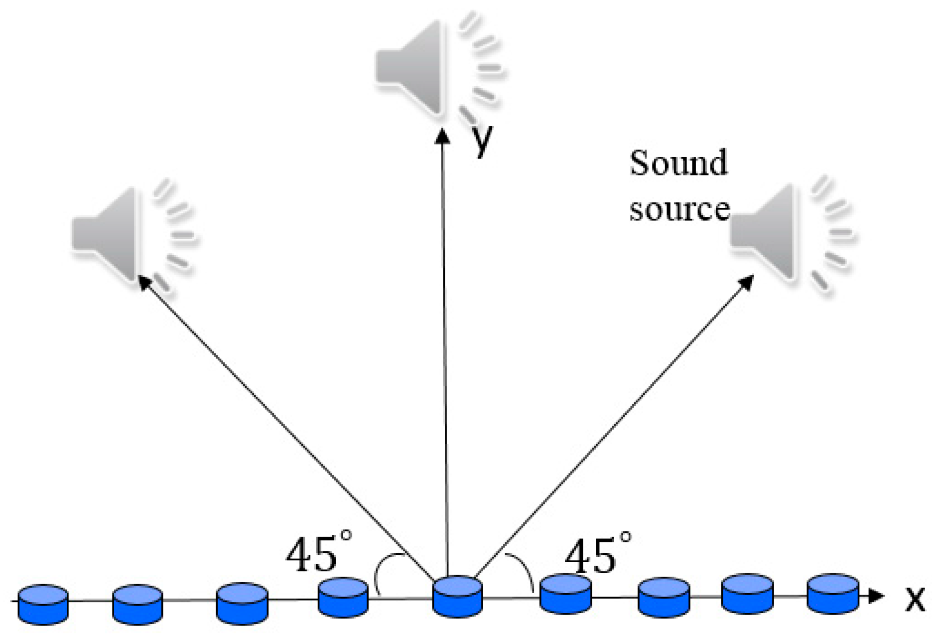
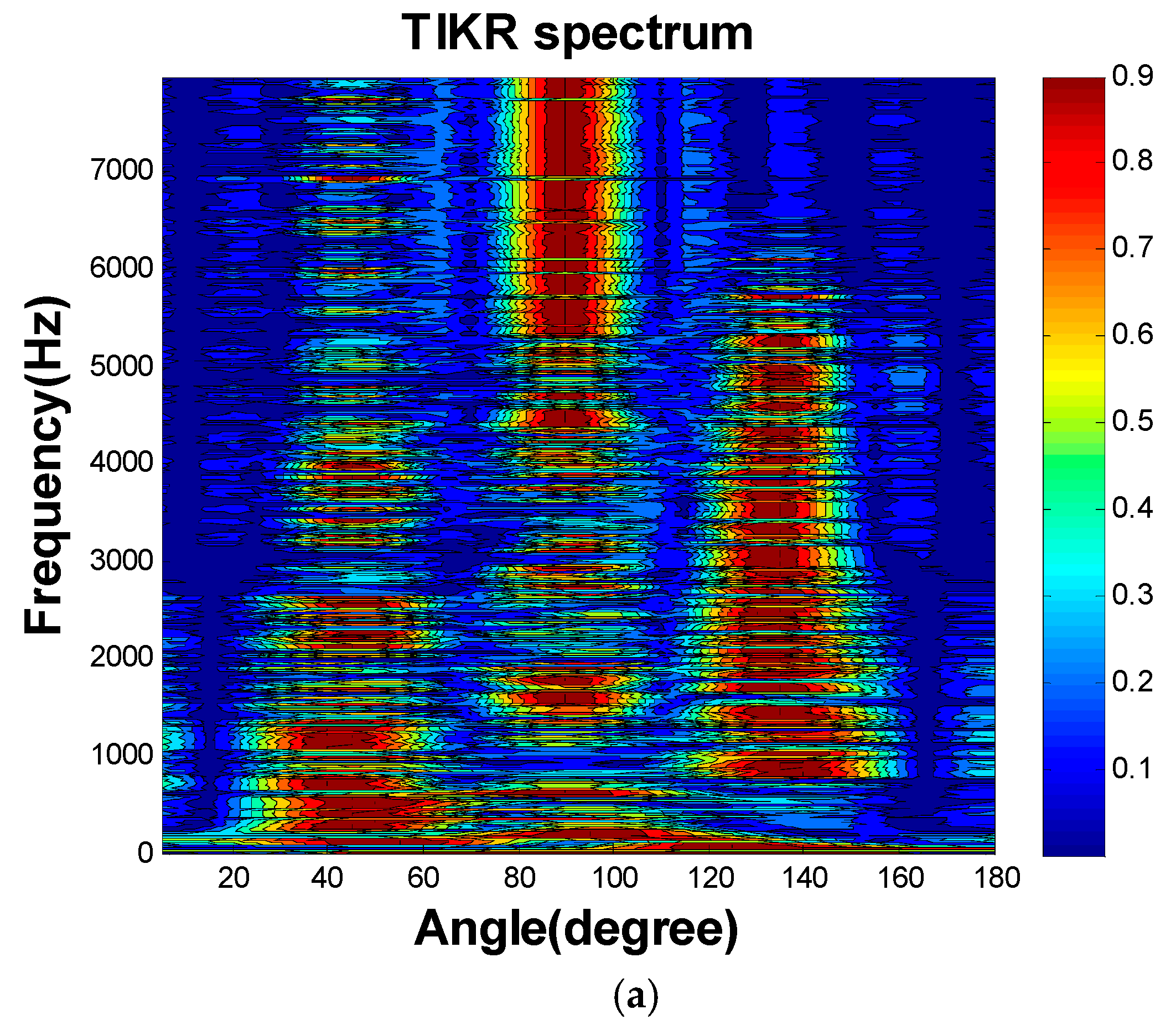
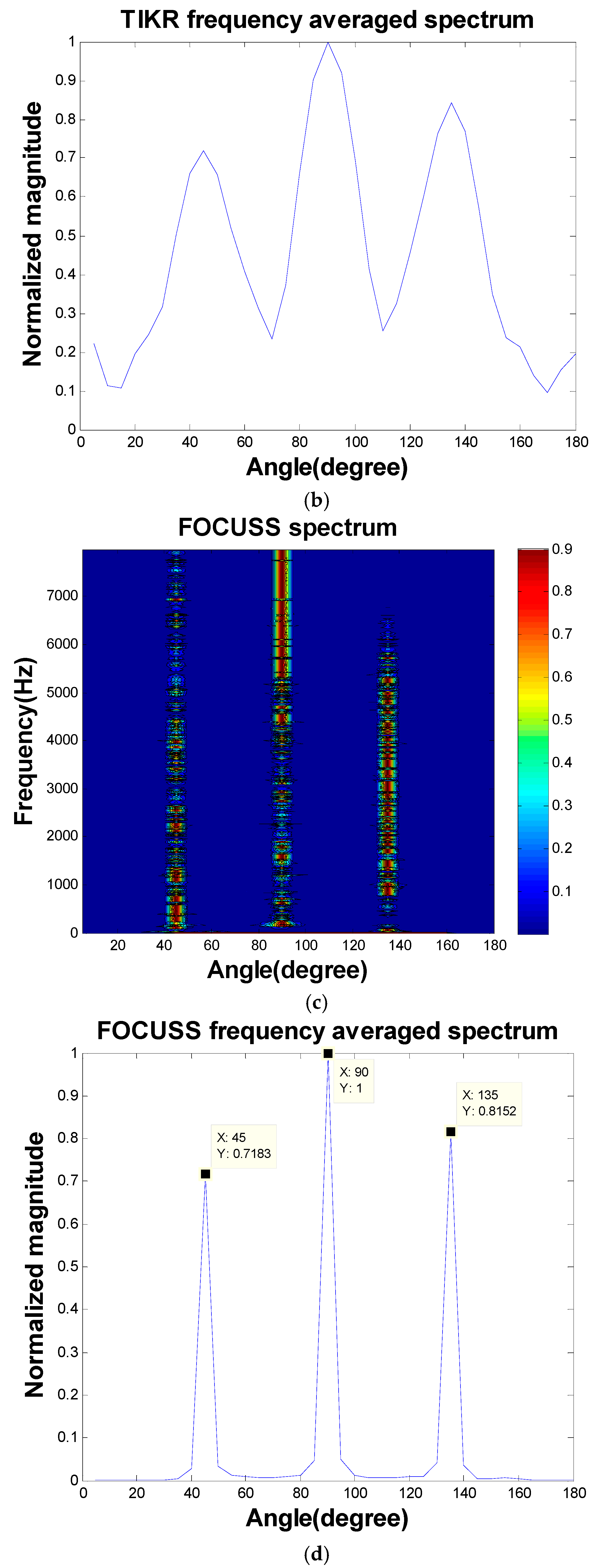
Figure 4, 10-microphone ULA was utilized to separate the signals emitted by three sources. The sources were located at the far field such that the plane wave assumption was valid. The spacing between adjacent microphones was 10 cm. This simulated underdetermined system contained 36 sources as our dictionary. We separated the signals and localized the signals in one stage. TIKR, FOCUSS, and CS-CVX algorithms were used to solve these inverse problems. Figure 5 shows the condition numbers of different frequencies. The problem is ill-conditioned at low frequencies. Source localization results are shown in Figure 6.
The separation results obtained using TIKR, FOCUSS, and CS-CVX are summarized in Table 1. PESQ is an objective test measure for speech quality evaluation. It is a full-reference algorithm and analyzes the speech signal sample-by-sample after a temporal alignment of corresponding excerpts of reference and test signal. The mean opinion score (MOS) is calculated on the basis of PESQ ranging from 1 to 5; MOS signifies the difference in speech quality between the clean and the separated signals, which is affected by separation performance and signal distortion. The segmental SNR (segSNR) is defined as
S N R s e g = 1 N k = 1 N 10 log 10 [ n f r a m e k | s ( n ) | 2 n f r a m e k | s ^ ( n ) s ( n ) | 2 ]
The segSNR correlates with the effect of noise reduction. The FOCUSS-PINV algorithm was observed to achieve the highest score in PESQ and segSNR (Table 1), although it required more computation time than TIKR and FOCUSS-TIKR.
In our previous simulation, we simulated microphones that had no noise; therefore, our regularization parameter was very close to zero. In the current simulation, our microphones did have white noise with a magnitude equal to the magnitude of the microphone signals divided by 100. Therefore, the potential loss of SNR was 40 dB.
The regularization parameter is chosen by the maximal singular σ 1 value dividing 100 in 100 Hz. In our case, the maximal singular value was equal to 5.32. Next, a coarse search was performed by varying β in orders of 10 and using the GSS algorithm to find the optimal regularization parameter. In this case, the optimal regularization parameter was 0.0174, and the FOCUSS-PINV of the robustness to the noise was very ineffective because PINV artifacts caused discontinuities in regularization. CS-CVX was sensitive to the noise, and the segSNR and PESQ achieved lower scores than FOCUSS-TIKR did, as listed in Table 2 and Table 3 (20dB). Therefore, noise was present, and FOCUSS-TIKR was the best choice in this case. It outperformed PESQ and segSNR.

3.2. Random Array

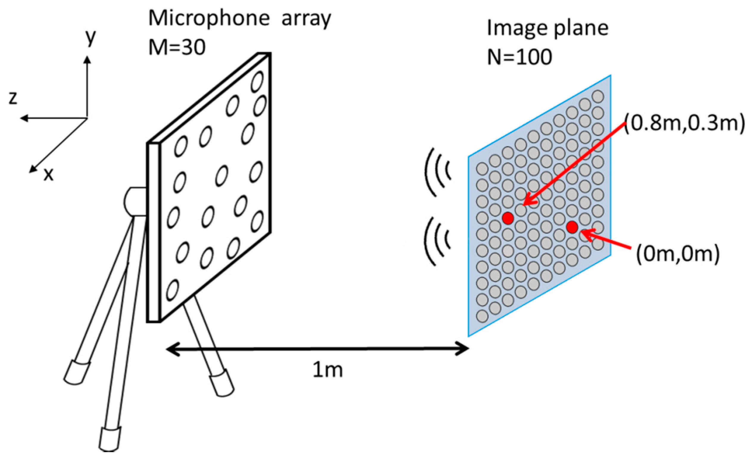
A simulation was conducted for localization and separation of two point sources located at (0, 0, −1 m) and (0.8, 0.3, −1 m), both of which were emitting clean speech signals, as illustrated in Figure 7. A 30-element random array with aperture dimension 0.48 m × 0.4 m situated at z = 0 was utilized to capture the signals emitted by these two sources. To set up the propagation matrix, 100 (10 × 10) equivalent sources were distributed on the image plane located 1 m away from the array. 
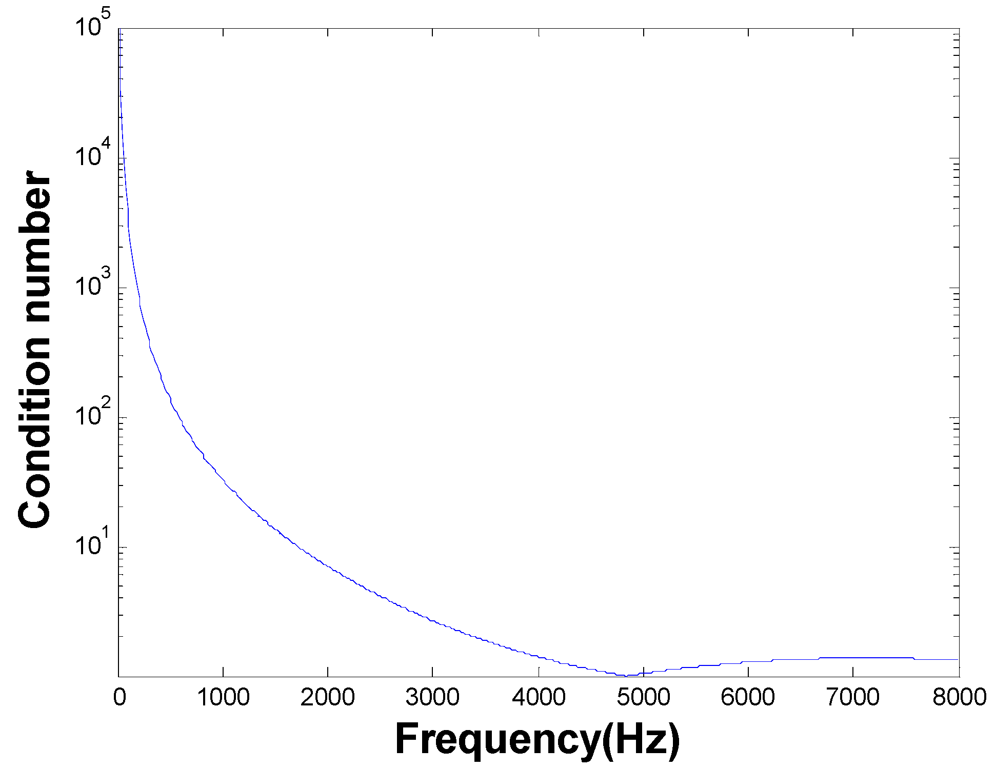
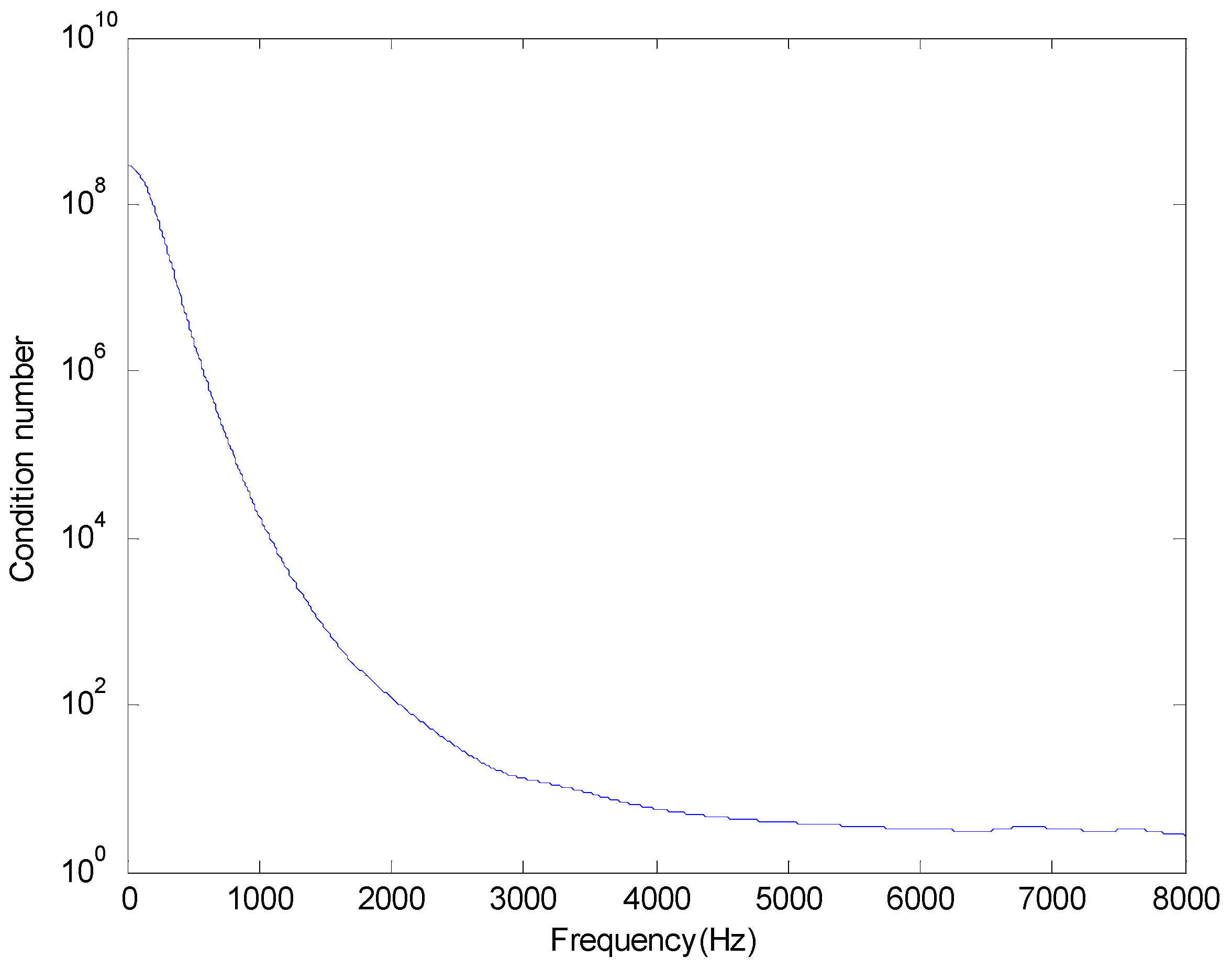
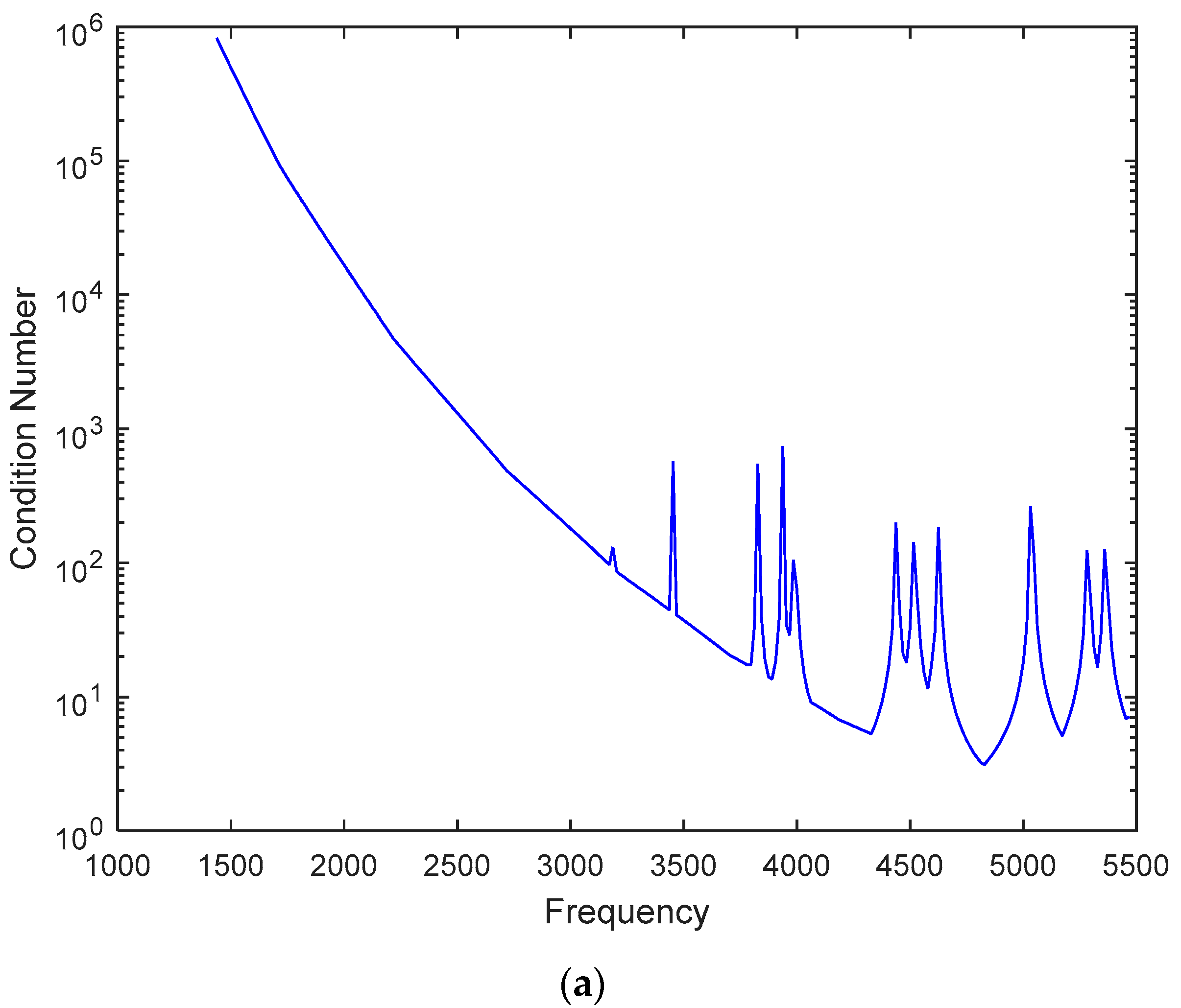
Figure 8 shows the condition numbers of different frequencies. The problem is ill-conditioned at low frequencies.
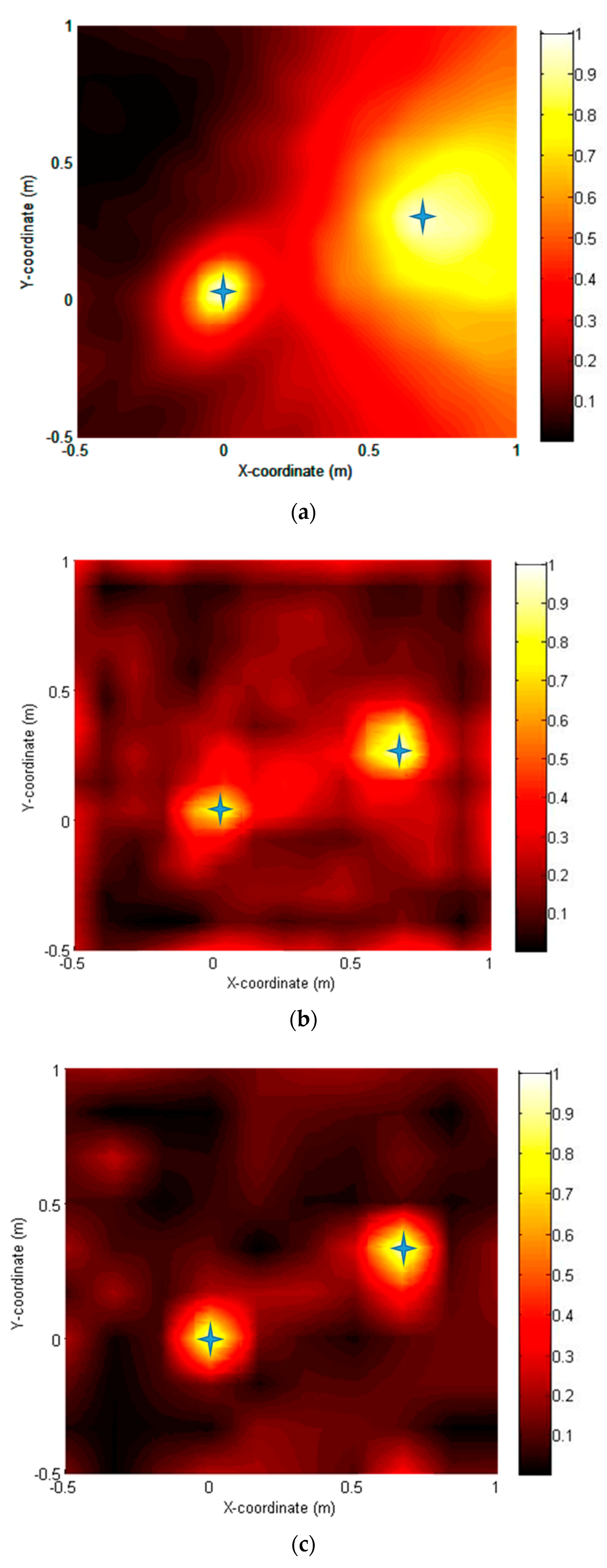
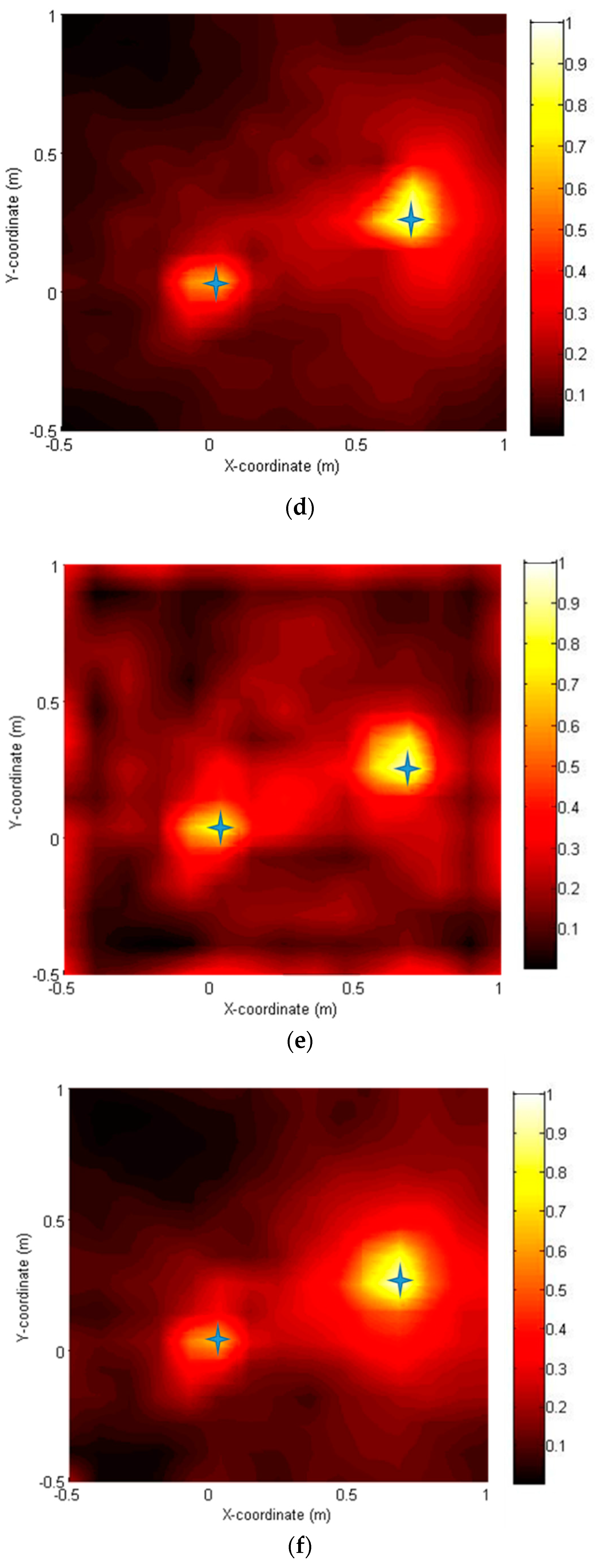
Figure 9a–f show the source localization results obtained using six approaches. Two sources were correctly located on the noise map with varying degrees of resolution by all methods. A conventional method delay and sum (DAS) method (a) gave the poorest resolution, whereas the CS-CVX method provided the highest resolution. The SD method (d) and CG method (f) were acceptable but did not perform quite as well as the CS-CVX method. The NT method (e) yielded accurate source locations with a slightly increased sidelobe level, but it was the most computationally efficient (Table 2).
Table 4 presents a comparison of the separation results obtained using five methods. CS-CVX displayed the highest scores for PESQ and segSNR, despite being extremely time-consuming. Iterative CS approaches were determined to be far more computationally efficient than the CS-CVX method. The CG method attained the highest PESQ, but the lowest segSNR. This suggests that the favorable separation performance of the CG method comes at the price of signal distortion. The SD and NT methods demonstrated acceptable PESQ and high segSNR. Although signals were not perfectly separated by using these two methods, the incurred distortion was minor. In general, methods present a trade-off between separation performance and signal distortion. Table 5 shows the separation results with additive noise (SNR = 28 dB). All the methods were observed to suffer from the interference of noise; consequently, the values of PESQ and segSNR were notably low. However, all the methods were determined to be robust to noise. The present study also considered mismatches between equivalent sources (dictionaries) and real sources. Table 6 shows the separation results of the NT method with different levels of mismatch. Mismatch means that the real source is not precisely on the deployed source location (dictionary). Extreme mismatch means the real source is exactly on the center of four nearest the deployed source location. More descriptions are added to the revised manuscript. Unless the source was just at the center of the near dictionaries, the separation performance was high and not influenced by noise.

3.3. SFA and SFS

Depending on the sparsity of the sound sources, the SFA stage can be implemented in several manners [35,36,37,38]. For the sparse-source scenario, a two-stage algorithm is utilized; the source bearings are estimated using the minimum power distortionless response (MPDR) [7] and the associated amplitudes of plane waves are estimated using the TIKR algorithm. For the nonsparse-source scenario, a one-stage algorithm based on the CS-CVX algorithm or the FOCUSS algorithm is employed.
The SFS stage is carried out using a loudspeaker array to reconstruct the sound field with the source bearing and amplitude obtained in the SFA stage. Pressure matching was employed for the SFS purpose in this study by sampling a large number of virtual control points in the interior area surrounded by the loudspeakers. The pressure matching procedure can be described as the following optimization problem:
min s s ( ω ) B ( ω ) s p ( ω ) H ( ω ) s s ( ω ) ,
where s p ( ω ) = [ s 1 ( ω ) s P ( ω ) ] T is the amplitude vector of the Pth primary plane-wave component, s s ( ω ) = [ s 1 ( ω ) s L ( ω ) ] T denotes the amplitude vector of the input signals to the L secondary loudspeaker sources, H ( ω ) K × L denotes the room response matrix, and b d = [ e j k d · y 1 e j k d · y K ] T is the steering vector for the dth primary plane-wave component to the nth control point, y n , n = 1 , , K . B ( ω ) = [ b 1 b d ] K × P is the steering matrix from the plane-wave components obtained in the preceding SFA stage to the control points. Therefore, the optimal solution can be written as
s s ( ω ) = H # ( ω ) B ( ω ) s p ( ω ) ,
where “#” symbolizes some type of inverse operation on the matrix H ( ω ) . In this study, TIKR was utilized to calculate the input signal amplitudes to the secondary sources. GSS can be used to find the optimal regularization parameter.
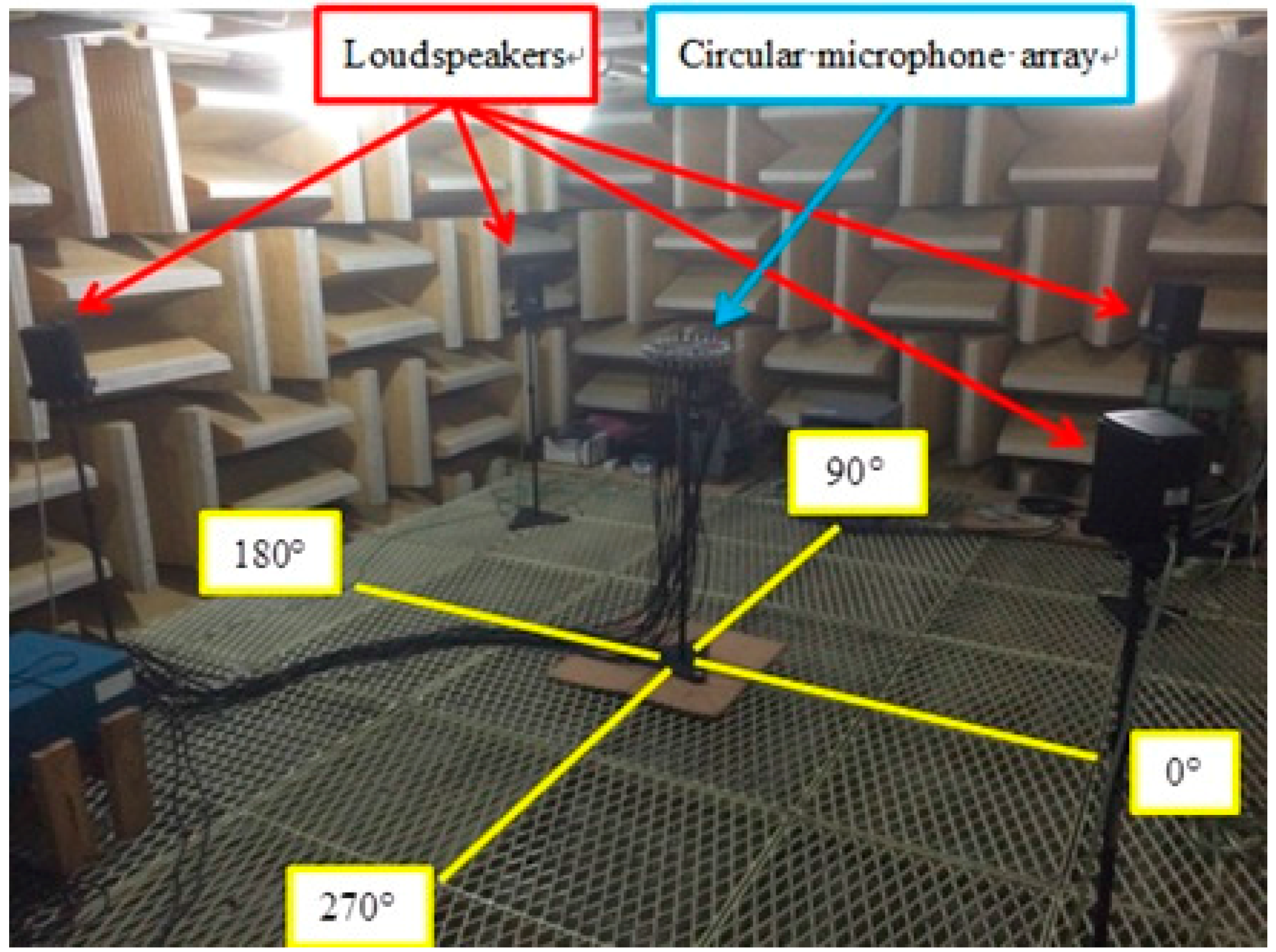
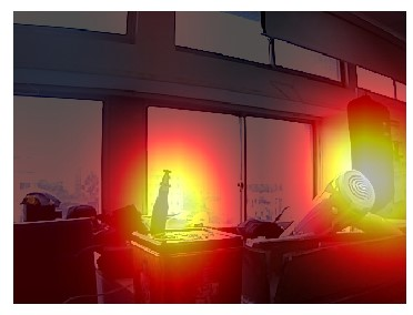
Experiments were conducted to validate the proposed audio analysis and synthesis system. In the SFA stage, a 24-element circular microphone array with a radius of 12 cm was utilized to capture and parameterize the sound field in an anechoic chamber (the recording room), as illustrated in 
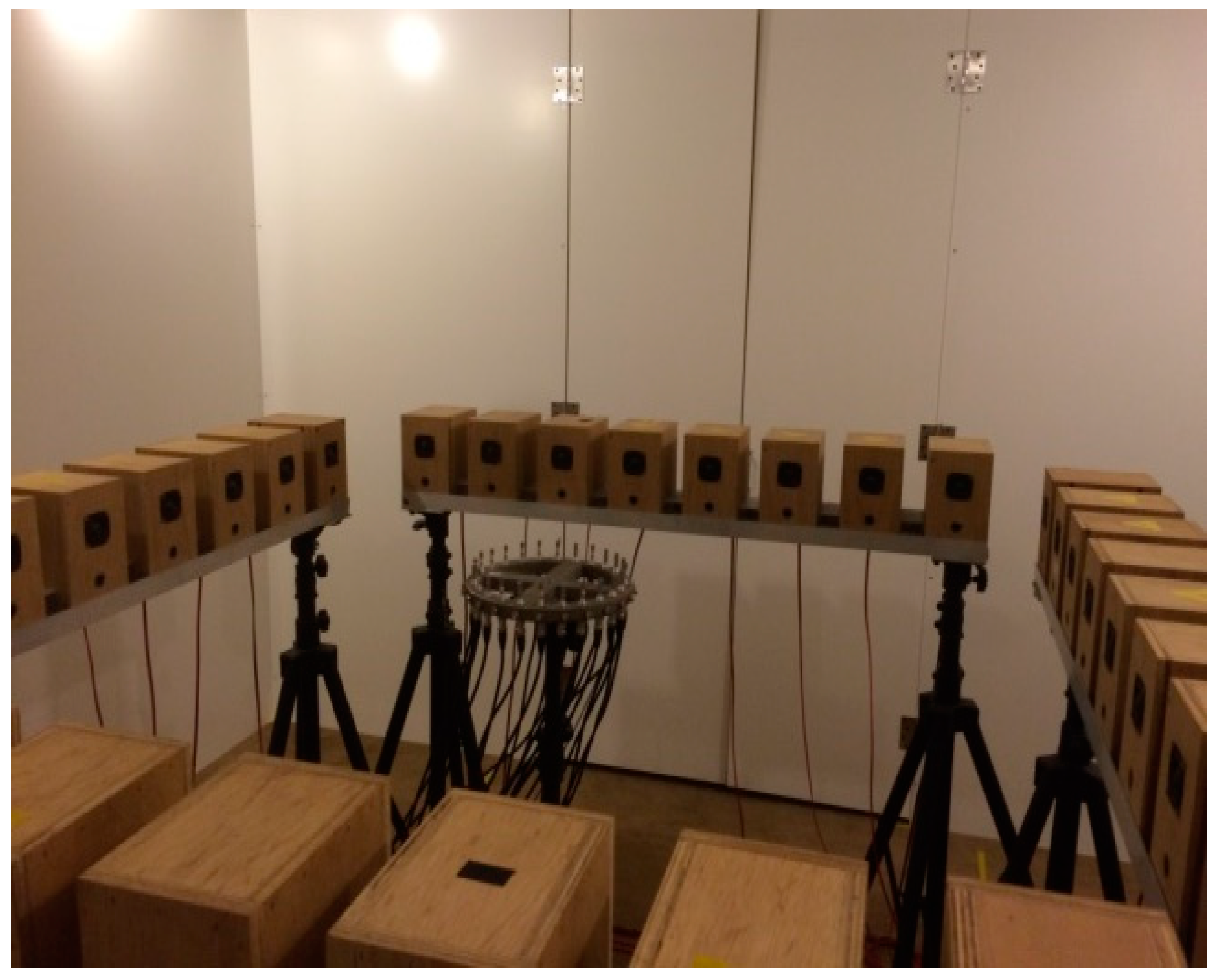
Figure 10. In the SFS stage, a rectangular, 32-loudspeaker array was employed to reproduce in a live room (the reproduction room) the sound field previously encoded in the SFA stage. The walls of the room were lined with acoustically reflective boards (Figure 11).
To process microphone output and loudspeaker input signals, multichannel analog-to-digital converters (M-32 AD) and digital-to-analog converters (M-32 DA) (RME, Haimhausen, Germany) were used with a sampling frequency of 16 kHz.
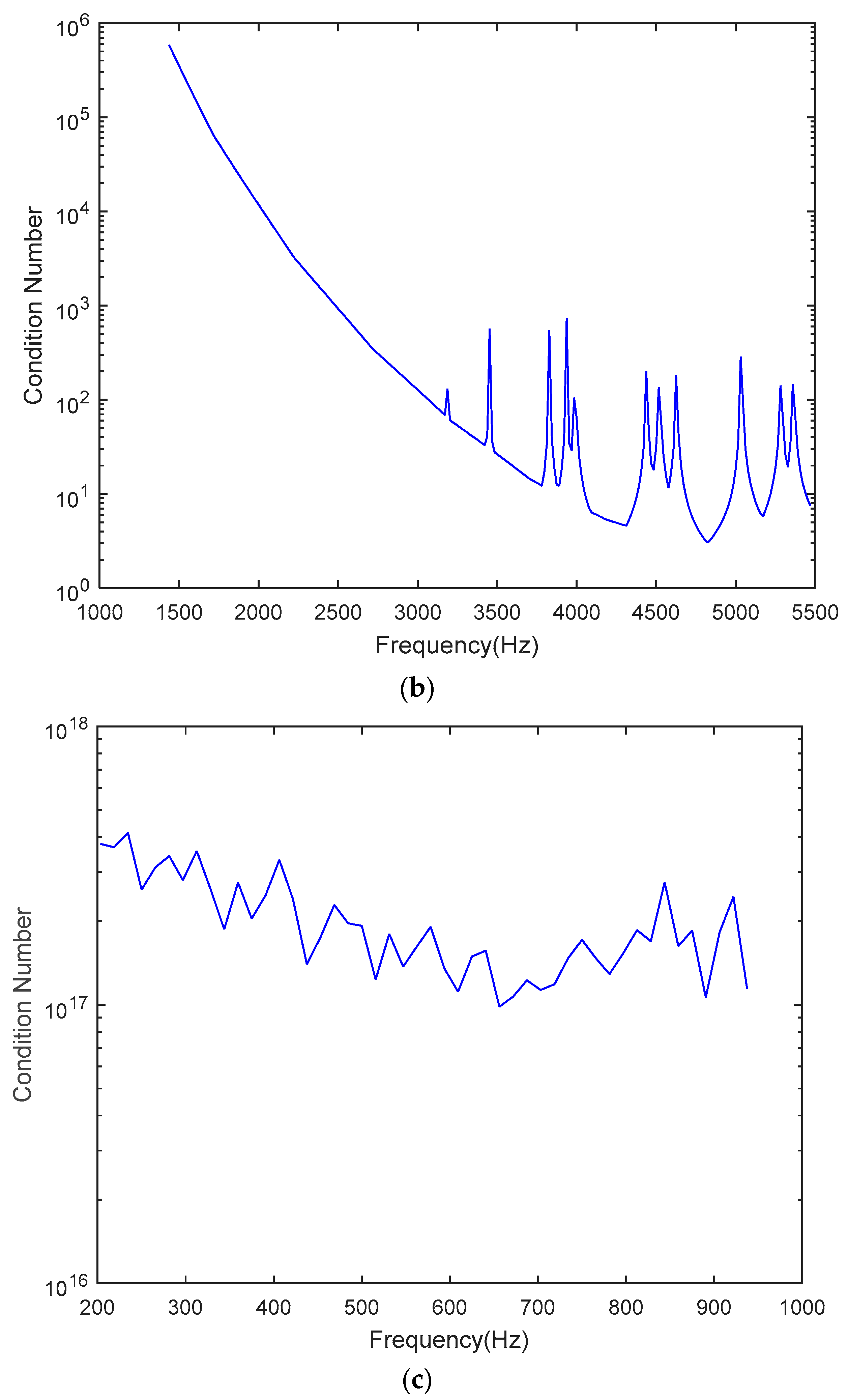
An audio codec system involves three inverse problems, namely the SFA stage, room response modeling, and the SFS stage. The condition numbers are plotted against the frequencies of three steering matrices in Figure 12a–c. Figure 12c indicates that the ill-posedness encountered in the room response modeling procedures must be addressed, with the aid of appropriate regularization methods. Large regularization parameters can increase the robustness of the inverse problem. In this study, we set the regularization parameter to 10.
In the SFA experiment, loudspeaker sources positioned at the angles θ = 60 ° , 240 ° 
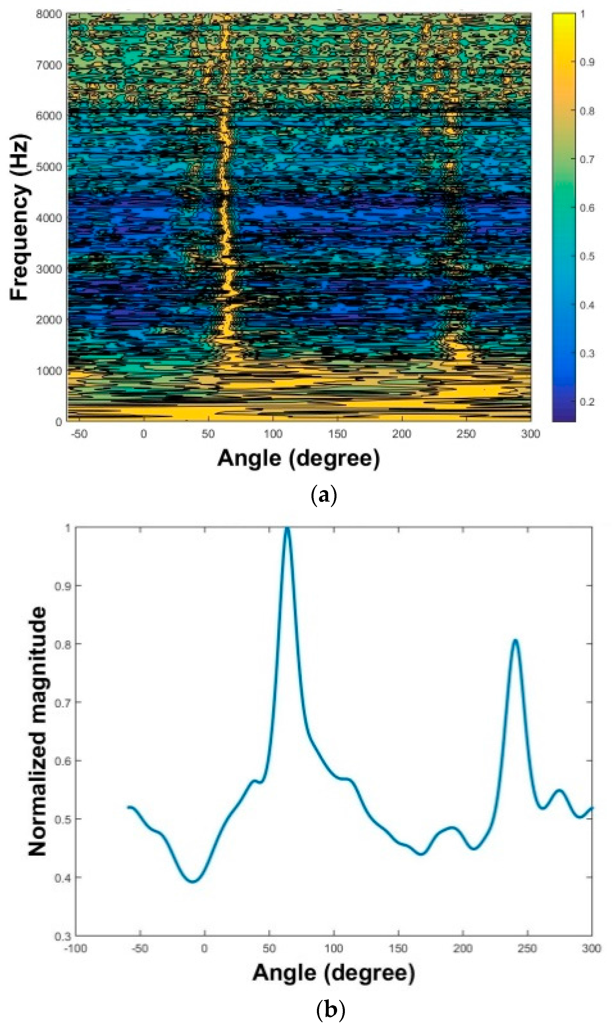
played two 10-s speech clips. After recording the source by CMA, we used three algorithms to extract the source signals. First, we applied the two-stage MPDR and TIKR algorithms. The MPDR spectrum is plotted as a function of angle and frequency in Figure 13a. The resulting frequency-averaged and normalized MPDR spectrum is illustrated in Figure 13b, which peaks at the angles θ = 60 ° , 240 ° as desired. The results show that the source was accurately localized using MPDR. Next, the source signals were extracted using the TIKR algorithm. We also applied one-stage CS algorithms and one-stage FOCUSS algorithms, which located sources and separated their amplitudes in a single calculation.
The signals extracted using different methods were evaluated by using the MOS of the PESQ test. Results confirmed that the TIKR performed well in signal separation with satisfactory audio quality. The results are summarized in Table 7.
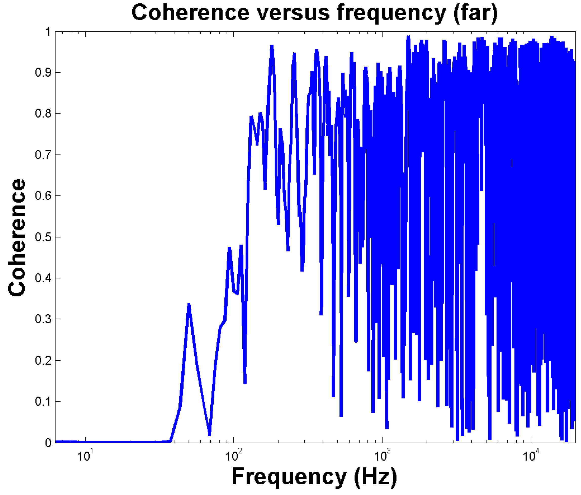
One sample coherence function between one loudspeaker and one microphone is shown in Figure 14, indicating the signal quality to be poor below 200 Hz. Therefore, band-limited processing was applied for all frequencies up to 200 Hz in the SFS stage. In this frequency range, pressure matching was used on the basis of the room response model.
The SFS stage was conducted for three different methods. The coherence between the loudspeaker and the microphone was poor below 200 Hz; therefore, the signals below 200 Hz were not processed. Method 1, band-limited processing, was applied from 200 Hz to the spatial aliasing frequency, 952 Hz, in the SFS stage. In this frequency range, pressure matching was performed on the basis of the room response model. Below 200 Hz, unprocessed audio signals were fed directly to the loudspeakers. Above 952 Hz, a simple vector panning [39] approach was adopted. The optimal regularization parameter β achieving the highest MOS in room response modeling was calculated using GSS [21] as β = 0.0008634.
In the second method, instead of a vector panning method, we used DAS to process signals above 952 Hz. In the third method, we used pressure matching to obtain signals above 200 Hz. The use of different regularization parameters in pressure matching results in different levels of localization performance and audio quality.
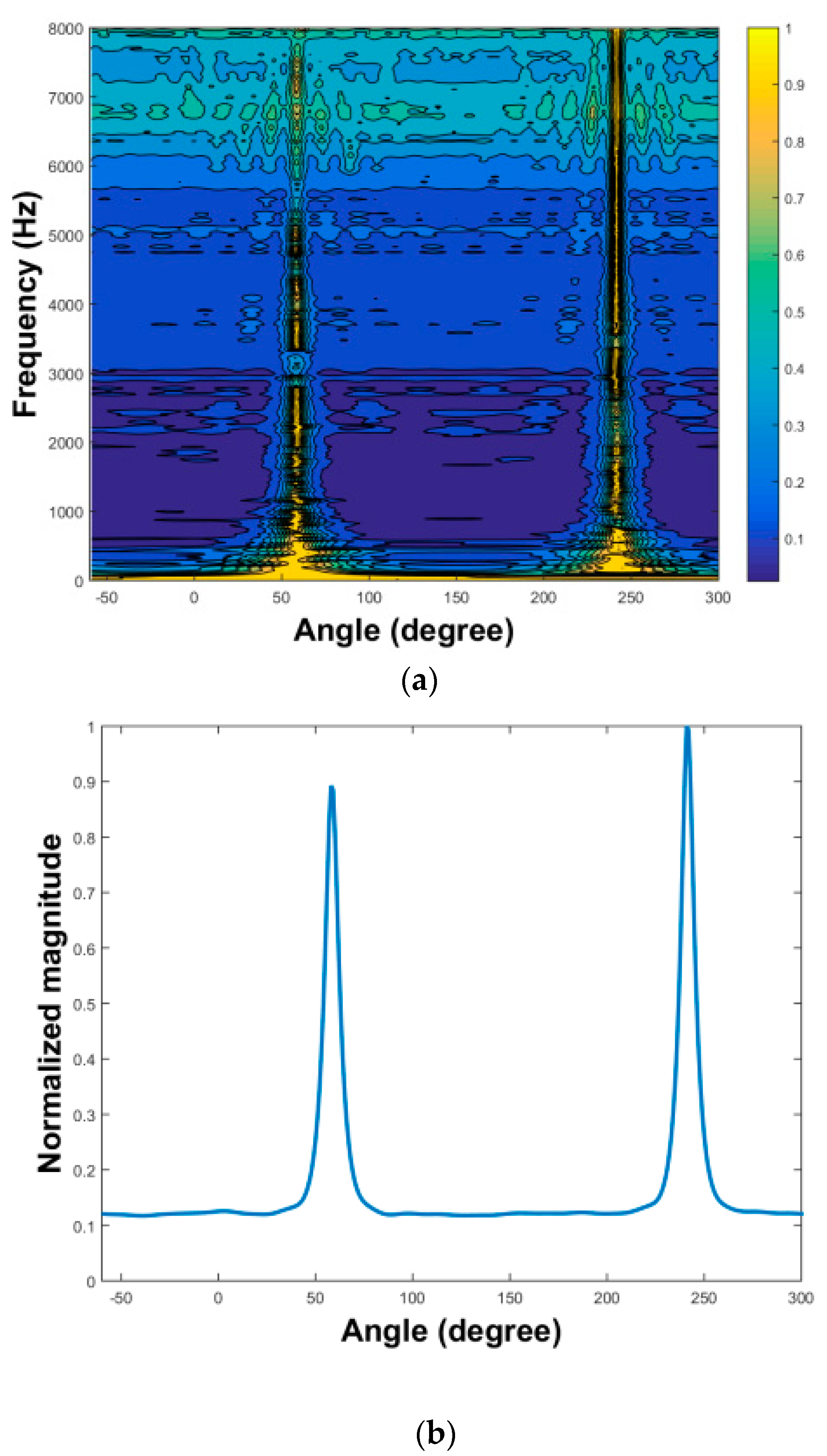
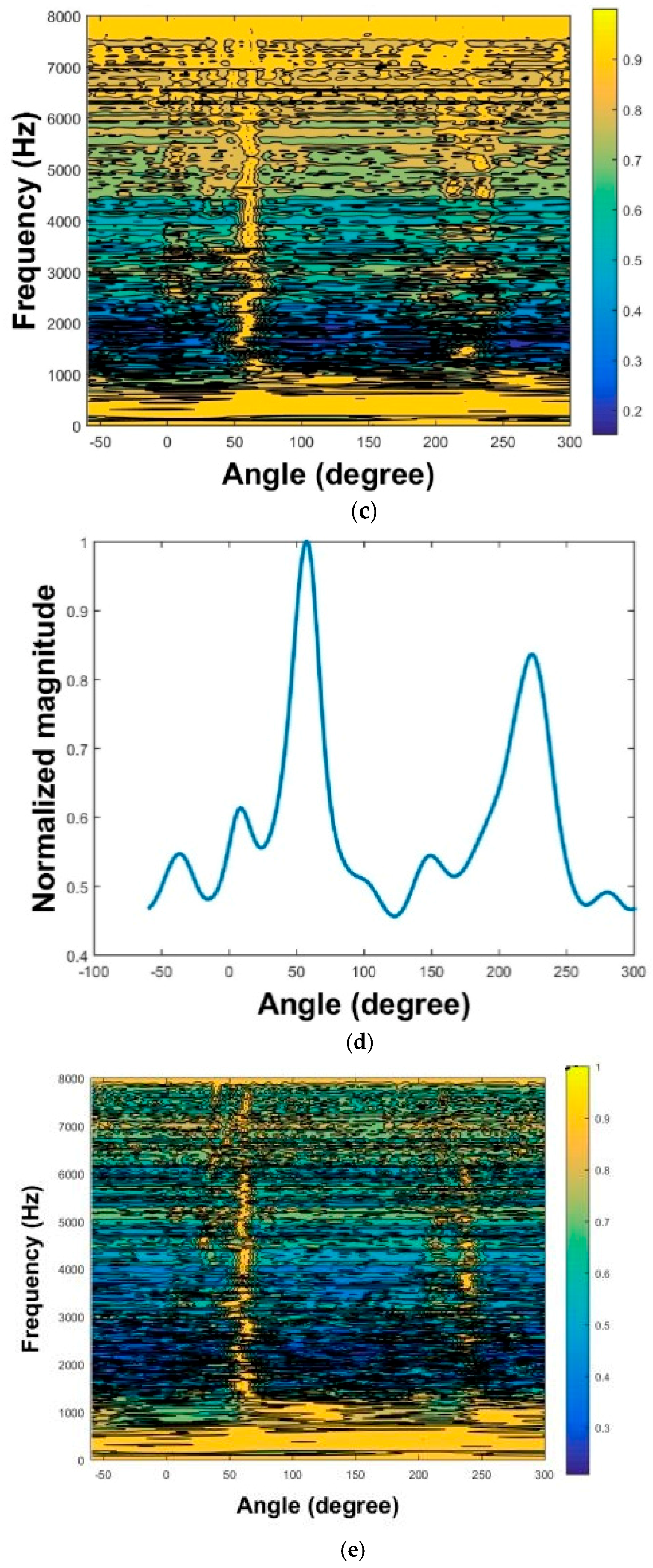
Figure 15a,c shows the MPDR spectrum and the normalized MPDR spectrum obtained using the third method for β = 0.01 and β = 10, respectively. Low values of the regularization parameter β yielded higher localization performance than high values did. These two signals were compared with the clean signal through the PESQ test. The results showed that the high β ensured satisfactory voice quality, whereas the low β impaired voice quality.
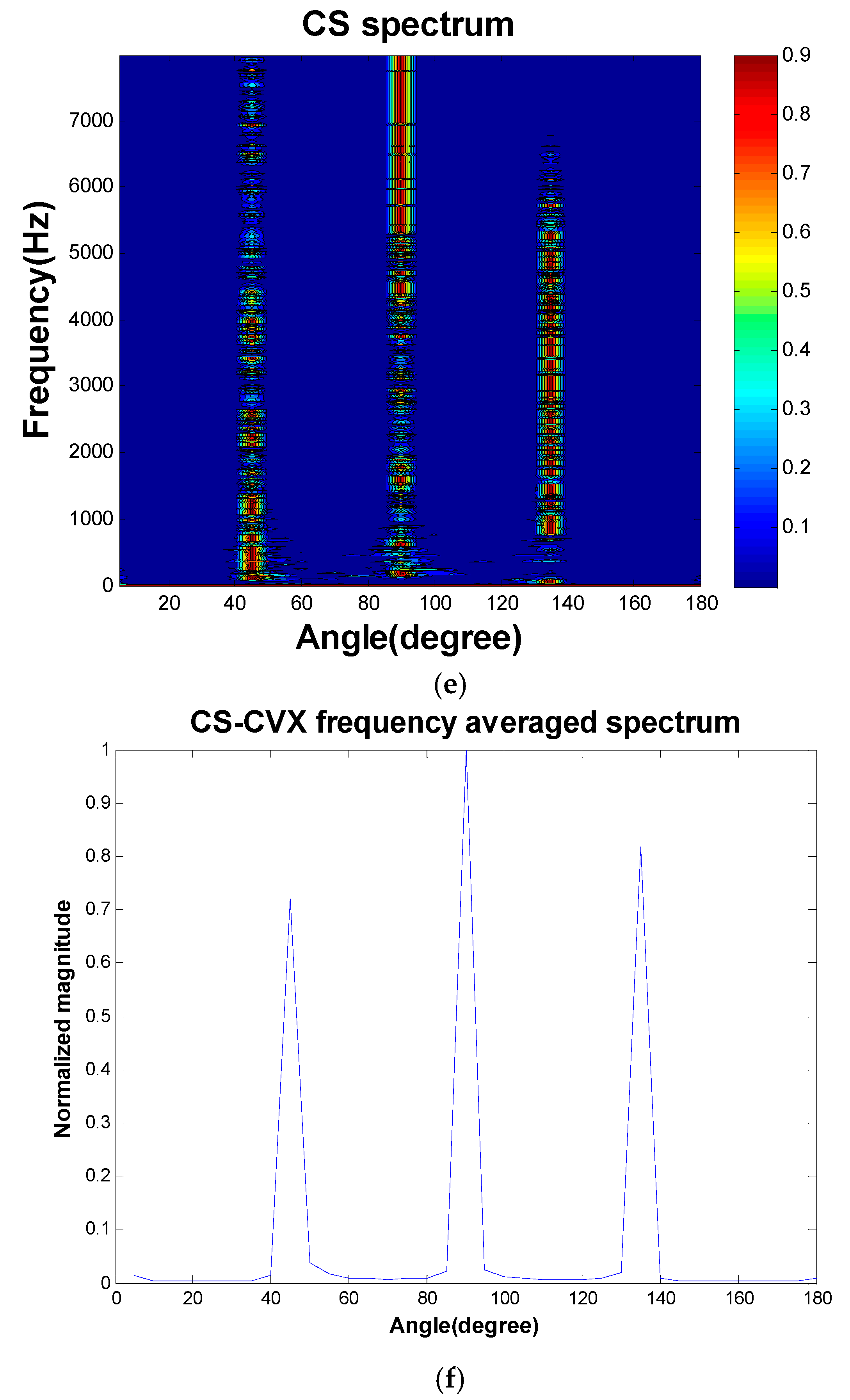
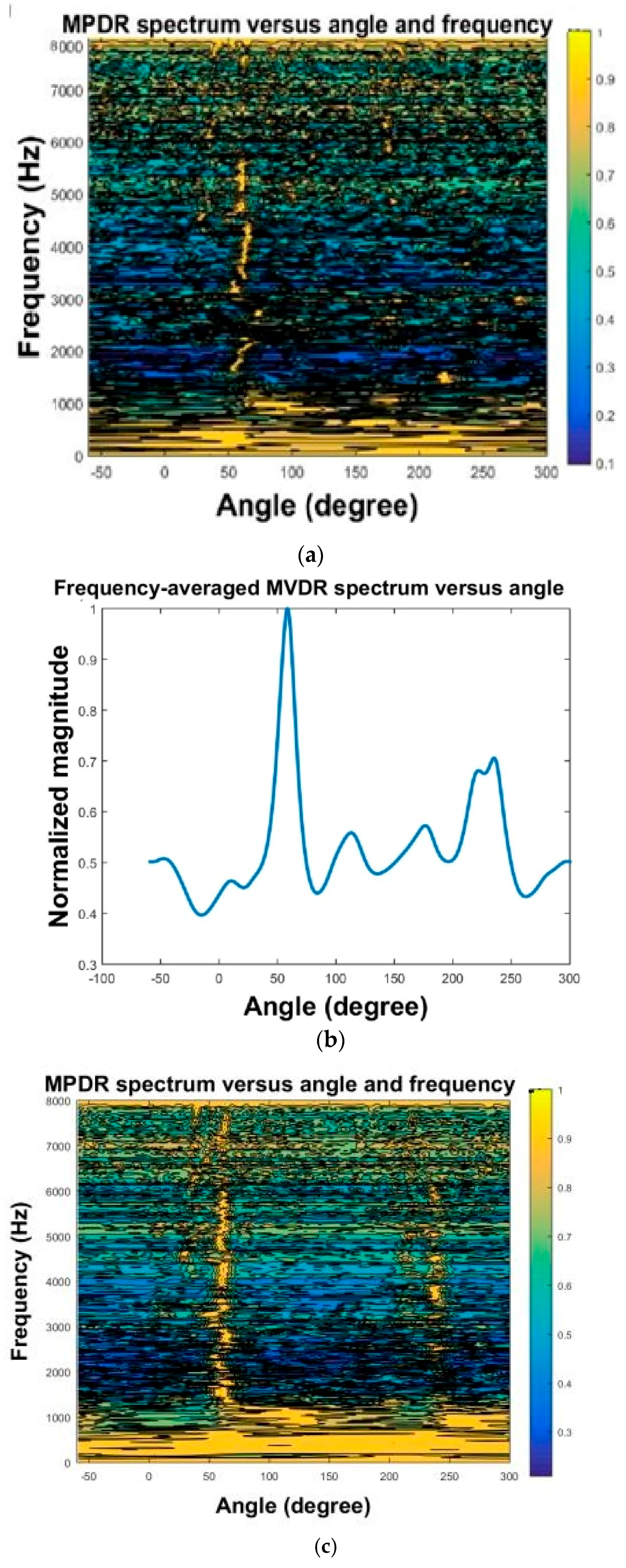
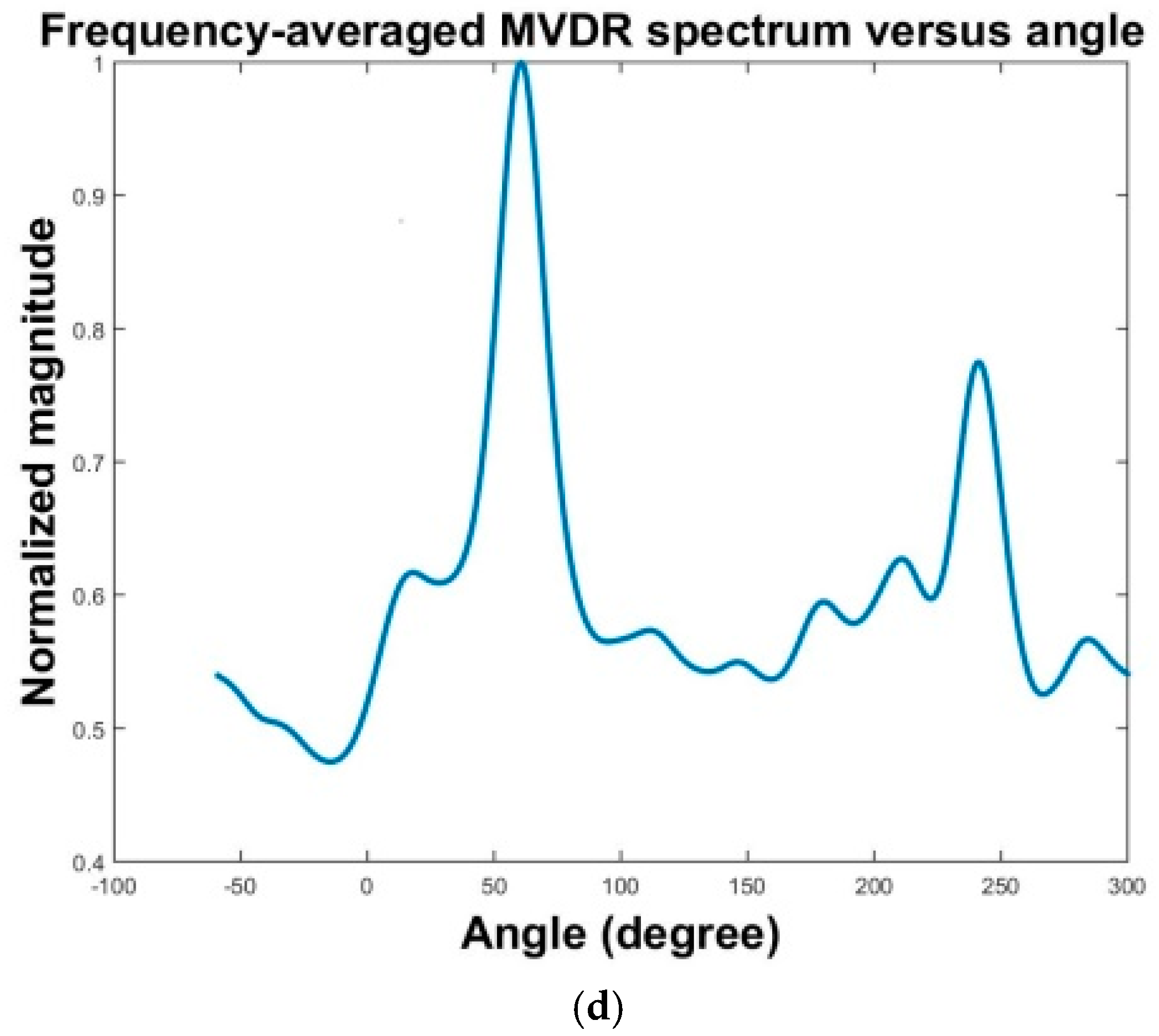
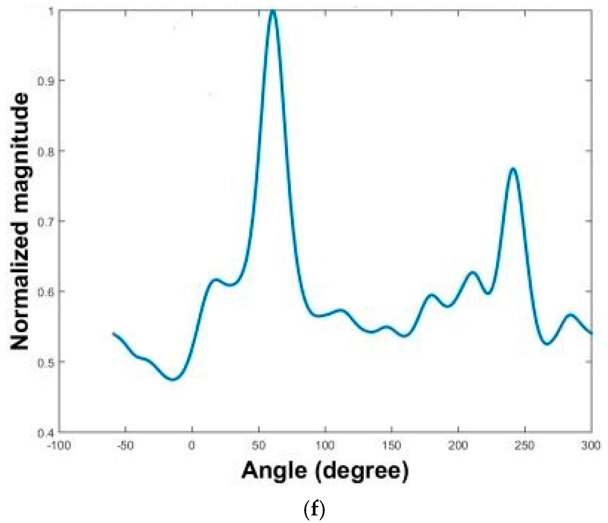
The results of three localization methods are presented in Figure 16a–f. The MPDR spectra are plotted as functions of angle and frequency in Figure 16a,c,f. The resulting frequency-averaged and normalized MPDR spectra are shown in Figure 16b,d,f.

4. Conclusions

This study developed algorithms for solving inverse problems generally encountered in spatial audio signal processing. The TIKR algorithm was shown to solve overdetermined problems. However, the regularization parameter in the TIKR method was not effectively chosen. This study thus presents a guideline for choosing the optimal regularization parameter β in the TIKR method. Specifically, choosing the optimal β involves dividing the maximal singular value at low frequency by the threshold and then running the simulation forward and backward for powers of 10 of β. Optimization methods such as GSS can be used by observing the trend of an objective function (such as PESQ). Some trade-offs must be made between localization performance and voice quality. In general, a high β results in a small solution norm with high voice quality, whereas a low β yields a small residual norm with high localization performance.
Inverse problems in noise sound source localization and separation problems can be solved by 1-stage and 2-stage (overdetermined and underdetermined), each of the 1-stage and 2-stage methods has its advantages and disadvantages. In general, the 1-stage methods provide both localization and separation results with good performance. The 2-stage methods give slightly better separation performance than the 1-stage methods. From our experience, PESQ correlates better with separability and segSNR correlates better with distortion.
For 1-stage (underdetermined) problems, iterative CS algorithms have been developed for solving acoustic inverse problems, with applications to localization and separation. The results demonstrate that the CS-CVX method was effective in solving CS problems, despite being computationally expensive. Iterative CS methods achieved comparable performance to the CS-CVX method for CS problems, in far less computation time. The FOCUSS-TIKR and CG methods attained high PESQ, whereas the SD and NT methods attained high segSNR. In general, iterative CS methods were determined to perform better than the TIKR method. For 1-stage methods, FOCUSS-TIKR attains the highest MOS value of PESQ for clean signals, while the Newton method performs the best. Both methods require less CPU time than the CS-CVX.
Inverse solution approaches are also useful in solving SFA and SFS problems. In this study, three inverse problems were solved for implementing an audio codec system. Because of the ill-posed yield at low frequencies, particularly in the room response modeling stage, choosing an appropriate regularization parameter β was crucial. Therefore, this stage required a larger regularization parameter than the SFA and SFS stages required. In the analysis stage, the one-stage CS algorithm was determined to be more computationally expensive than the two-stage TIKR algorithm. In the synthesis stage, the first method performed well in localization, but did not perform well in reproduced voice quality. As compared with the third method, the second method reproduced signals with boosted high-frequency content above 952 Hz with poor localization. The third method had the highest performance in terms of voice quality and localization performance.

Acknowledgments

The work was supported by the Ministry of Science and Technology (MOST) of Taiwan, Republic of China, under project number 102-2221-E-007-029-MY3.

Author Contributions

M.R. Bai and C.-M. Yang conceived and designed the experiments; Y.-H. Chiang and P.-C. Wu performed the experiments; P.-C. Wu and C. Chung analyzed the data; C. Chung and Y.-H. Chinag wrote the paper.

Conflicts of Interest

The authors declare no conflict of interest.

References

  1. Kim, Y.; Nelson, P.A. Spatial resolution limits for the reconstruction of acoustic source strength by inverse methods. J. Sound Vib. 2003, 265, 583–608. [Google Scholar] [CrossRef]
  2. Nelson, P.A.; Yoon, S.H. Estimation of acoustic source strength by inverse methods: Part I, conditioning of the inverse problem. J. Sound Vib. 2000, 233, 639–664. [Google Scholar] [CrossRef]
  3. Kim, Y.; Nelson, P.A. Optimal regularisation for acoustic source reconstruction by inverse methods. J. Sound Vib. 2004, 275, 463–487. [Google Scholar] [CrossRef]
  4. Maynard, J.D.; Williams, E.G.; Lee, Y. Nearfield acoustic holography: I. Theory of generalized holography and the development of NAH. J. Acoust. Soc. Am. 1985, 78, 1395–1413. [Google Scholar] [CrossRef]
  5. Hald, J. Fast wideband acoustical holography. J. Acoust. Soc. Am. 2016, 139, 1508–1517. [Google Scholar] [CrossRef] [PubMed]
  6. Brooks, T.F.; Humphreys, W.M. A deconvolution approach for the mapping of acoustic sources (DAMAS) determined from phased microphone arrays. J. Sound Vib. 2006, 294, 856–879. [Google Scholar] [CrossRef]
  7. Bai, M.R.; Kuo, C.H. Deconvolution-based acoustic source localization and separation algorithms. J. Acoust. Soc. Am. 2014, 135, 2358. [Google Scholar] [CrossRef]
  8. Bai, M.R.; Hua, Y.H.; Kuo, C.H.; Hsieh, Y.H. An integrated analysis-synthesis array system for spatial sound fields. J. Acoust. Soc. Am. 2015, 137, 1366–1376. [Google Scholar] [CrossRef] [PubMed]
  9. Bai, M.R.; Hsu, H.S.; Wen, J.C. Spatial sound field synthesis and upmixing based on the equivalent source method. J. Acoust. Soc. Am. 2014, 135, 269–282. [Google Scholar] [CrossRef] [PubMed]
  10. Elliott, S.J.; Cheer, J.; Murfet, H.; Holland, K.R. Minimally radiating sources for personal audio. J. Acoust. Soc. Am. 2010, 128, 1721–1728. [Google Scholar] [CrossRef] [PubMed]
  11. Bai, M.R.; Hsieh, Y.H. Point focusing using loudspeaker arrays from the perspective of optimal beamforming. J. Acoust. Soc. Am. 2015, 137, 3393–3410. [Google Scholar] [CrossRef] [PubMed]
  12. Bai, M.R.; Tung, C.W.; Lee, C.C. Optimal design of loudspeaker arrays for robust cross-talk cancellation using the Taguchi method and the genetic algorithm. J. Acoust. Soc. Am. 2005, 117, 2802–2813. [Google Scholar] [CrossRef] [PubMed]
  13. Loizou, P.C. Speech Enhancement: Theory and Practice; Taylor & Francis: Park Drive, UK; Abingdon, UK, 2007. [Google Scholar]
  14. Shabtai, N.R. Optimization of the directivity in binaural sound reproduction beamforming. J. Acoust. Soc. Am. 2015, 138, 3118–3128. [Google Scholar] [CrossRef] [PubMed]
  15. Miyoshi, M.; Kaneda, Y. Inverse filtering of room acoustic. IEEE Transac. Acoust. Speech Signal Process. 1998, 36, 145–152. [Google Scholar] [CrossRef]
  16. Groetsch, C.W. The Theory of Tikhonov Regularization for Fredholm Equations of the First Kind; Pitman Advanced Pub. Program: Boston, MA, USA, 1984. [Google Scholar]
  17. Hansen, P.C. Rank-Deficient and Discrete Ill-Posed Problems; Society for Industrial and Applied Mathematics: Philadelphia, PA, USA, 1998. [Google Scholar]
  18. Bertero, M.; Poggio, T.; Torre, V. Ill-Posed Problems in Early Vision. Proc. IEEE 1988, 76, 869–889. [Google Scholar] [CrossRef]
  19. Hansen, P.C. Analysis of Discrete Ill-Posed Problems by Means of the L-Curve; Society for Industrial and Applied Mathematics: Philadelphia, PA, USA, 1992. [Google Scholar]
  20. Hansen, P.C.; O’leary, D.P. The Use of the L-Curve in the Regularization of Discrete Ill-Posed Problems; Society for Industrial and Applied Mathematics: Philadelphia, PA, USA, 1993. [Google Scholar]
  21. Brent, R.P. Algorithms for Minimization without Derivatives; Prentice-Hall, Inc.: Englewood Cliffs, HJ, USA, 1973; pp. 48–75. [Google Scholar]
  22. Candes, J.; Wakin, M.B. An introduction to compressive sampling. IEEE Signal Process. Mag. 2008, 25, 21–30. [Google Scholar] [CrossRef]
  23. Edelmann, G.F.; Gaumond, C.F. Beamforming using compressive sensing. J. Acoust. Soc. Am. 2011, 130, 232–237. [Google Scholar] [CrossRef] [PubMed]
  24. Boyd, S.; Vandenberghe, L. Convex Optimization; Cambridge University Press: New York, NY, USA, 2004; Chapters 1–7. [Google Scholar]
  25. Bai, M.R.; Chen, C.C. Application of Convex Optimization to Acoustical Array Signal Processing. J. Sound Vib. 2013, 332, 6596–6616. [Google Scholar] [CrossRef]
  26. Grant, M.; Boyd, S. CVX, Version 1.21 MATLAB Software for Disciplined Convex Programming. Available online: http://cvxr.com/cvx (accessed on 14 June 2013).
  27. Gorodnitsky, I.F.; Rao, B.D. Sparse Signal Reconstruction from Limited Data Using FOCUSS: A Re-weighted Minimum Norm Algorithm. IEEE Trans. Signal Process. 1997, 45, 600–616. [Google Scholar] [CrossRef]
  28. ITU-T Recommendation P.862. Perceptual Evaluation of Speech Quality (Pesq): An Objective Method for End-to-End Speech Quality Assessment of Narrow-Band Telephone Networks and Speech Codecs; International Telecommunication Union: Geneva, Switzerland, 2001; p. 21. [Google Scholar]
  29. Bai, M.R.; Ih, J.G.; Benesty, J. Acoustic Array Systems: Theory, Implementation, and Application, 1st ed.; Wiley-IEEE Press: Singapore, 2013; Chapters 3–4. [Google Scholar]
  30. Golub, G.H.; van Loan, C.F. Matrix Computations, 3rd ed.; Johns Hopkins University Press: Baltimore, MD, USA, 1989; Chapter 12. [Google Scholar]
  31. Noble, B.; Daniel, J.W. Applied Linear Algebra; Prentice Hall: Englewood, NJ, USA, 1977. [Google Scholar]
  32. Hestenes, M.R.; Stiefel, E. Methods of conjugate gradients for solving linear systems. J. Res. Natl. Bur. Stand. 1952, 49, 409–436. [Google Scholar] [CrossRef]
  33. Fraysse, V.; Giraud, L. A Set of Conjugate Gradient Routines for Real and Complex Arithmetics; CERFACS Technical Report TR/PA/00/47; Cedex: Toulouse, France, 2000. [Google Scholar]
  34. Ginn, K.B.; Haddad, K. Noise source identification techniques: Simple to advanced applications. Proc. Acoust. 2012, 2012, 1781–1786. [Google Scholar]
  35. Capon, J. High-Resolution Frequency-Wavenumber Spectrum Analysis. Proc. IEEE 1969, 57, 1408–1418. [Google Scholar] [CrossRef]
  36. Gomes, J.; Hald, J.; Juhl, P.; Jacobsen, F. On the Applicability of the Spherical Wave Expansion with a Single Origin for Near-Field Acoustical Holography. J. Acoust. Soc. Am. 2009, 125, 1529–1537. [Google Scholar] [CrossRef] [PubMed]
  37. Candes, J.; Romberg, J.; Tao, T. Stable Signal Recovery from Incomplete and Inaccurate Measurements. Commun. Pure Appl. Math. 2006, 59, 1207–1223. [Google Scholar] [CrossRef]
  38. Candes, J.; Romberg, J.; Tao, T. Robust Uncertainty Principles: Exact Signal Reconstruction Form Highly Incomplete Frequency Information. IEEE Trans. Inf. Theory 2006, 52, 489–509. [Google Scholar] [CrossRef]
  39. Kim, Y.H.; Choi, J.W. Sound Visualization and Manipulation; Wiley: Singapore, 2013. [Google Scholar]
Figure 1. Schematic of golden section search. If f(β2) is higher than f(β4), β 3 is equal to β4 in the next iteration.
Applsci 07 00582 g001
Figure 2. Pruning process to promote sparsity of inverse solution.
Applsci 07 00582 g002
Figure 3. Flowchart of iterative compressive sampling algorithms (adapted from reference [5]).
Applsci 07 00582 g003
Figure 4. Numerical simulation of 10-microphone uniform linear array utilized to separate the signals emitted by three sources. The first source, located at θ = 45 ° , was broadcasting a male speech signal. The second source, located at θ = 90 ° , was broadcasting a female speech signal. The third source, located at θ = 135 ° , was broadcasting a music signal.
Applsci 07 00582 g004
Figure 5. Condition number versus frequency.
Applsci 07 00582 g005
Figure 6. Source localization results obtained using the focal underdetermined system solver (FOCUSS) algorithm and a uniform linear array. (a) Tikhonov regularization (TIKR) spectrum (b) TIKR averaged spectrum (c) FOCUSS spectrum (d) FOCUSS frequency-averaged spectrum. (e) Compressive sampling-convex optimization (CS-CVX) spectrum (f) CS-CVX frequency-averaged spectrum.
Applsci 07 00582 g006aApplsci 07 00582 g006bApplsci 07 00582 g006c
Figure 7. Arrangement for simulation of localization and separation of two sources.
Applsci 07 00582 g007
Figure 8. Condition number versus frequency.
Applsci 07 00582 g008
Figure 9. Localization results of two point sources. (a) Delay and sum algorithm, (b) Tikhonov regularization algorithm, (c) compressive sampling-convex optimization algorithm, (d) steepest descent algorithm, (e) Newton’s algorithm, and (f) conjugate gradient algorithm.
Applsci 07 00582 g009aApplsci 07 00582 g009b
Figure 10. Sound field analysis experimental arrangement in a 5.4 m × 3.5 m × 2 m anechoic room.
Applsci 07 00582 g010
Figure 11. Sound field synthesis experimental arrangement in a 3.6 m × 3.6 m × 2 m live room fitted with reflective walls.
Applsci 07 00582 g011
Figure 12. Plots of condition numbers versus frequencies of each steering matrix in three inverse problems: (a) sound field analysis stage; (b) room response modeling; and (c) sound field synthesis stage.
Applsci 07 00582 g012aApplsci 07 00582 g012b
Figure 13. Localization of one music source signal with sampling rate 16 kHz, located at the angles 60 ° ,   240 ° in an anechoic chamber. By using a uniform circular array with a radius of 12 cm, the source direction can be identified by the peak in the angular spectrum. (a) Minimum power distortionless response (MPDR) spectrum plotted versus angle and frequency. (b) Frequency-averaged and normalized MPDR spectrum.
Applsci 07 00582 g013
Figure 14. Coherence curve measured from one loudspeaker to one microphone in a live room. A PULSE analysis platform made from Brüel & Kjær was arranged to measure the coherence curve. A white noise signal with sampling rate 16 kHz was used as the driving signal of the loudspeaker.
Applsci 07 00582 g014
Figure 15. Localization results in the sound field synthesis experiment by the third method with different regularization parameters. β = 10 (a,b) and β = 0.01 (c,d).
Applsci 07 00582 g015aApplsci 07 00582 g015b
Figure 16. Localization results in the sound field synthesis experiment with three different approaches. (a,b) first method, (c,d) second method, and (e,f) third method.
Applsci 07 00582 g016aApplsci 07 00582 g016bApplsci 07 00582 g016c
Table 1. Separation performance of the Tikhonov regularization (TIKR) and focal underdetermined system solver (FOCUSS) methods for three sources in the underdetermined system.
MethodsTIKRFOCUSS-PINVFOCUSS-TIKRCS-CVX
PESQSource 12.0343.9663.3503.251
Source 21.6963.1462.8792.783
Source 31.9123.8183.3943.347
segSNRSource 10.55411.9211.278.817
CPU time (s)5381048716302
Table 2. Separation performance of the Tikhonov regularization (TIKR), focal underdetermined system solver (FOCUSS), and compressive sampling-convex optimization (CS-CVX) methods for three sources with additive white noises (40dB SNR).
MethodsTIKRFOCUSS-PINVFOCUSS-TIKRCS-CVX
PESQSource 12.1351.1702.9412.412
Source 21.8101.1212.2341.321
Source 31.7231.1682.8412.241
segSNRSource 10.52−10.001.5580.946
CPU time (s)5881749716431
Table 3. Separation performance of the TIKR, FOCUSS and CS-CVX methods for three sources with additive white noises (20dB SNR).
MethodsTIKRFOCUSS-PINVFOCUSS-TIKRCS-cvx
PESQSource 11.5121.1682.5121.436
Source 21.4011.1182.0121.712
Source 31.4891.0442.4871.324
segSNRSource 1−0.12−13.110.12−1.112
CPU time (s)5781549416421
Table 4. Separation performance of five algorithms for two speech sources.
MethodsTIKRCS-CVXSDNTCG
PESQSource 11.993.122.392.482.76
Source 22.603.312.772.833.13
segSNRSource 12.157.545.086.040.50
Source 22.738.247.027.261.53
CPU time (s)20131065377296386
Table 5. Separation performance of five algorithms for two speech sources with additive noise.
MethodsTIKRCS-CVXSDNTCG
PESQSource 11.822.832.222.382.59
Source 22.123.202.532.532.88
segSNRSource 11.402.112.034.13−0.50
Source 22.306.512.091.721.23
CPU time (s)21131348358290307
Table 6. Separation performance of Newton’s algorithm for two speech sources with different mismatch conditions.
Methodswithout Mismatchwith MismatchExtreme Mismatch
PESQSource 12.522.482.14
Source 22.812.831.70
segSNRSource 16.906.04−0.40
Source 26.337.260.18
Table 7. Mean opinion score of perceptual evaluation of speech quality for source signal separation at the angles 60 ° ,   240 ° with speech signals using Tikhonov regularization (TIKR), compressive sampling-convex optimization (CS-CVX), and focal underdetermined system solver (FOCUSS).
MethodsTwo-Stage TIKROne-Stagecs-CVXOne-Stagefocuss
PESQSource 12.843.111.56
Source 22.792.991.61
segSNRSource 117.4020.7413.54
Source 216.5917.3412.68
CPU time (s)827,588275

