Detection of Pitting in Gears Using a Deep Sparse Autoencoder

Abstract

In this paper; a new method for gear pitting fault detection is presented. The presented method is developed based on a deep sparse autoencoder. The method integrates dictionary learning in sparse coding into a stacked autoencoder network. Sparse coding with dictionary learning is viewed as an adaptive feature extraction method for machinery fault diagnosis. An autoencoder is an unsupervised machine learning technique. A stacked autoencoder network with multiple hidden layers is considered to be a deep learning network. The presented method uses a stacked autoencoder network to perform the dictionary learning in sparse coding and extract features from raw vibration data automatically. These features are then used to perform gear pitting fault detection. The presented method is validated with vibration data collected from gear tests with pitting faults in a gearbox test rig and compared with an existing deep learning-based approach.

1. Introduction

Gears are one of the most critical components in many industrial machines. Health monitoring and fault diagnosis of gears are necessary to reduce breakdown time and increase productivity. Pitting is one of the most common gear faults and normally difficult to detect. An undetected gear pitting fault during the operation of the gears can lead to catastrophic failures of the machines.

In recent years, many gear pitting fault detection methods have been developed. Following the same way to classify machine fault diagnostic and prognostic methods by [1,2], gear pitting fault detection methods can be classified into two main categories, namely model-based methods and data-driven methods. The model-based techniques rely on accurate dynamic models of the systems, while the data-driven approaches use data to train fault detection models. Model-based approaches obtain the residuals between actual system and output. These residuals are then used as the indicator of the actual faults [3,4]. However, the model-based approaches require not only expertise in dynamic modeling, but also accurate condition parameters of the studied system. On the other hand, data-driven approaches do not require the knowledge of the target system and dynamic modeling expertise. In comparison with model-based techniques, data-driven approaches can design a fault detection system that can be easily applied when massive data is available. Data-driven techniques are appropriate when a comprehensive understanding of system operation is absent, or when it is sufficiently difficult to model the complicated system [5].

Data-driven-based gear pitting fault detection methods in general relies on feature extraction by human experts and complicated signal processing techniques. For example, Reference [6] used a zoomed phase map of continuous wavelet transform to detect minor damage such as gear fitting. References [7,8] used the mean frequency of a scalogram to get features for gear pitting fault detection. Reference [9] extracted condition indicators from time-averaged vibration data for gear pitting damage detection. Reference [10] used empirical mode decomposition (EMD) to extract features from vibration signals for gear pitting detection. Reference [11] combined EMD and fast independent component analysis to extract features from stator current signals for gear pitting fault detection. Reference [12,13] applied spectral kurtosis to extract features for gear pitting fault detection. Reference [14] extracted statistical parameters of vibration signals in the frequency domains as an input to artificial neural network for gear pitting fault classification. One challenge facing the abovementioned data-driven gear fault detection methods in the era of big data is that features extracted from vibration signals depend greatly on prior knowledge of complicated signal processing and diagnosis expertise. Besides, features are selected per the specific fault detection problems and may not be appropriate for different fault detection problems. An approach that can automatically and effectively self-learns gear fault features from the big vibration data and effectively detect the gear fault is necessary to address the challenge.

As a data-driven approach, sparse coding is a class of unsupervised methods for learning sets of overcomplete bases to represent data efficiently. Unlike principal component analysis (PCA) that learn a complete set of basis vectors efficiently, sparse coding learns an overcomplete basis. This gives sparse coding the advantage of generating basis vectors that are able to better capture structures and patterns inherent in the input data. Recently, sparse coding-based methods have been developed for machinery fault diagnosis [15,16,17,18]. However, these methods used manually constructed overcomplete dictionaries that cannot guarantee to match the structures in the analyzed data. Sparse coding with dictionary learning is viewed as an adaptive feature extraction method for machinery fault diagnosis [19]. Study reported in Reference [19] developed a feature extraction approach for machinery fault diagnosis using sparse coding with dictionary learning. In their approach, the dictionary is learned through solving a joint optimization problem alternatively: one for the dictionary and one for the sparse coefficients. One limitation with this approach is that solving the joint optimization problem alternatively for massive data is NP-complete [20] and therefore is not efficient for automation.

In this paper, a new method is proposed. The proposed approach combines the advantages of sparse coding with dictionary learning in feature extraction and the self-learning power of the deep sparse autoencoder for dictionary learning. Autoencoder is an unsupervised machine learning technique and a deep autoencoder is a stacked autoencoder network with multiple hidden layers. To the knowledge of the authors, no attempt to combine sparse coding with dictionary learning and deep sparse autoencoder for gear pitting fault detection has been reported in the literature.

2. The Methodology

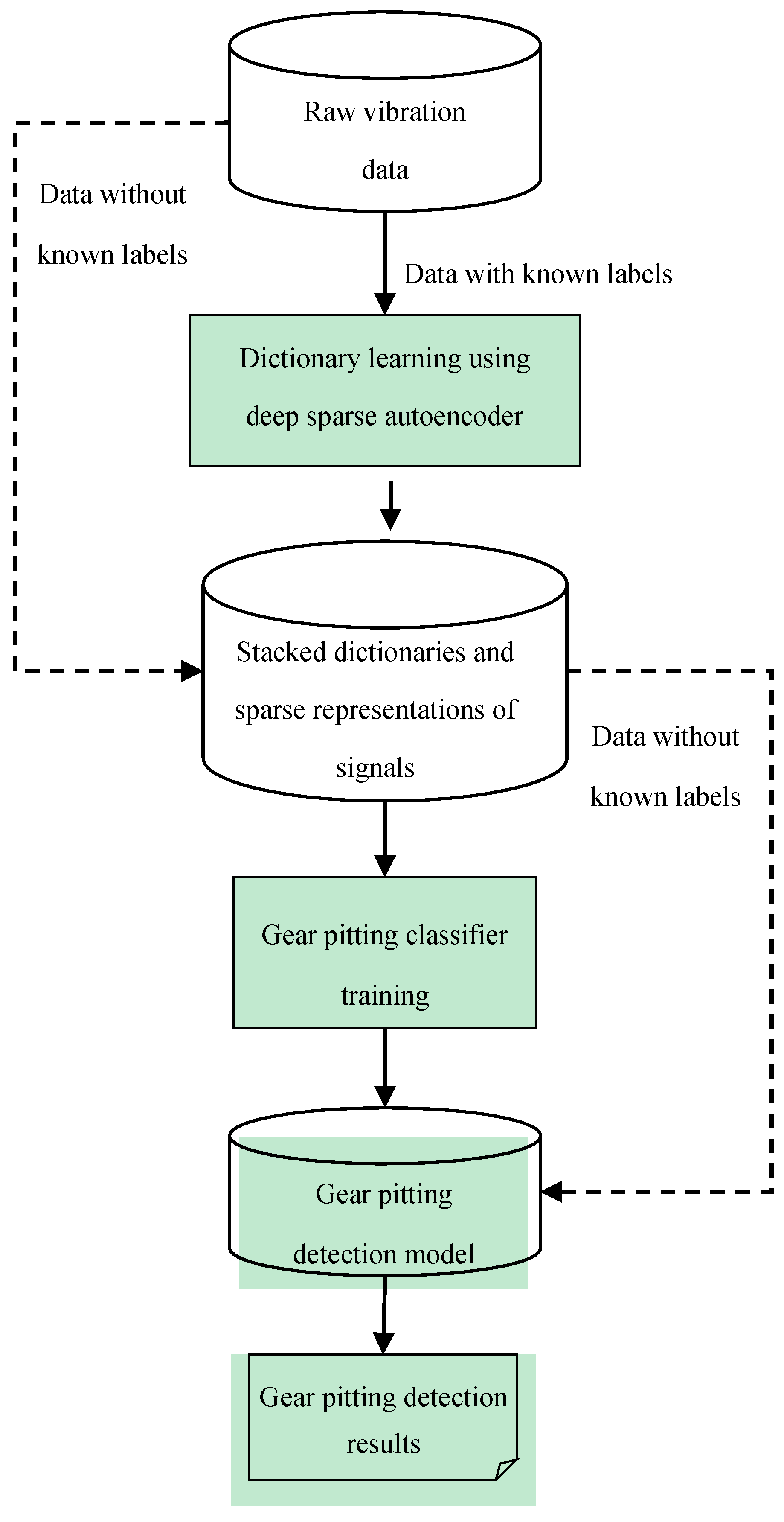
The general procedure of the presented method is shown in Figure 1 below. As shown in Figure 1, the presented method is composed of three main steps. Firstly, the dictionary and the corresponding representation of raw data will be obtained through unsupervised learning by the deep sparse autoencoder. Then, a simple backpropagation neural network constructed as the last hidden layer and the output layer is trained to classify the healthy and pitting gear condition using the learnt representation. With the learnt dictionary and trained classifier, the testing raw data are then imported into the network for pitting fault detection. It should be noted that the dictionary learning process is an unsupervised learning process. Thus, the representations regarded as features extracted from raw signals are learnt completely unsupervised without fine-tuning. Section 2.1 and Section 2.2 give a brief introduction on dictionary learning and autoencoder, respectively. Dictionary learning using deep sparse autoencoder for gear pitting detection is explained in Section 2.3.

2.1. Dictionary Learning

In recent years, the application of dictionary learning has been popularized in various fields, including image and speech recognition [21,22,23,24,25]. The study of dictionary learning application in vision can be traced back to the end of the last century [26]. The goal of dictionary learning is to learn a basis for representation of the original input data. The expansion of dictionary learning based applications is benefited from the introduction of K-SVD [27,28]. K-SVD is an algorithm that decomposes the training data in matrix form into a dense basis and sparse coefficients. Given an input signal $\mathit{x}={\left[x_1,x_2,\dots ,x_n\right]}^T$, the basic dictionary learning formula can be expressed as:

$$\underset{\mathit{D},\mathit{S}}{\min }{\Vert \mathit{x}-\mathit{D}\mathit{S}\Vert }_2^2$$

(1)

where $\mathit{D}\in {ℝ}^{n\times K}$ represents the dictionary matrix to be learnt with dimension n as number of data points in the input signal $\mathit{x}$ and $K$ as the number of atoms in the dictionary D, each column of D the basic function ${\mathit{d}}_k$ also known as atoms in dictionary learning, $\mathit{S}={\left[s_1,s_2,\dots ,s_k\right]}^T$ the representation coefficients of the input signal $\mathit{x}$, and $\Vert ·{\Vert }_2$ the approximation accuracy accessed by the $l^{2}norm$.

The goal of dictionary learning is to learn a basis which can represent the samples in a sparse presentation, meaning that $\mathit{S}$ is required to be sparse. Thus, fundamental principle of dictionary learning with sparse representations is expressed as:

$$\underset{\mathit{S}}{\min }{\Vert \mathit{S}\Vert }_0$$

(2)

Subject to:

$${\Vert \mathit{x}-\mathit{D}\mathit{S}\Vert }_2^2\le \gamma$$

(3)

where function ${\Vert ·\Vert }_0$ is referred to as $l_{0}norm$ that counts the nonzero entries of a vector, as a sparsity measurement, and $\gamma$ the approximation error tolerance.

As shown in Equation (2), solution of the $l_{0}norm$ minimization is a NP hard problem [20]. Thus, the orthogonal matching pursuit (OMP) [29] is commonly used to solve approximation of $l_{0}norm$ minimization. As mentioned previously, the popular used dictionary learning algorithm K-SVD was developed with employment of OMP as well. The K-SVD is constituted by two main procedures. In the first procedure, the dictionary matrix is firstly learnt and then it is used in the second procedure to represent the data sparsely. In the procedure of dictionary learning, K-SVD estimate the atoms one at a time according to the ranking update with efficient technique. Such strategy leads to the disadvantage of K-SVD as relatively low computing efficiency since the singular value decomposition (SVD) is required in each iteration.

The basic functions of dictionary matrix D can be either manually extracted or automatically learned from the input data. The manually extracted basic functions are simple and will lead to fast algorithms, however with poor performance on matching the structure in the analyzed data. An adaptive dictionary should be learned from input data through machine learning based methods, such that the basic functions can capture a maximal amount of structures of the data.

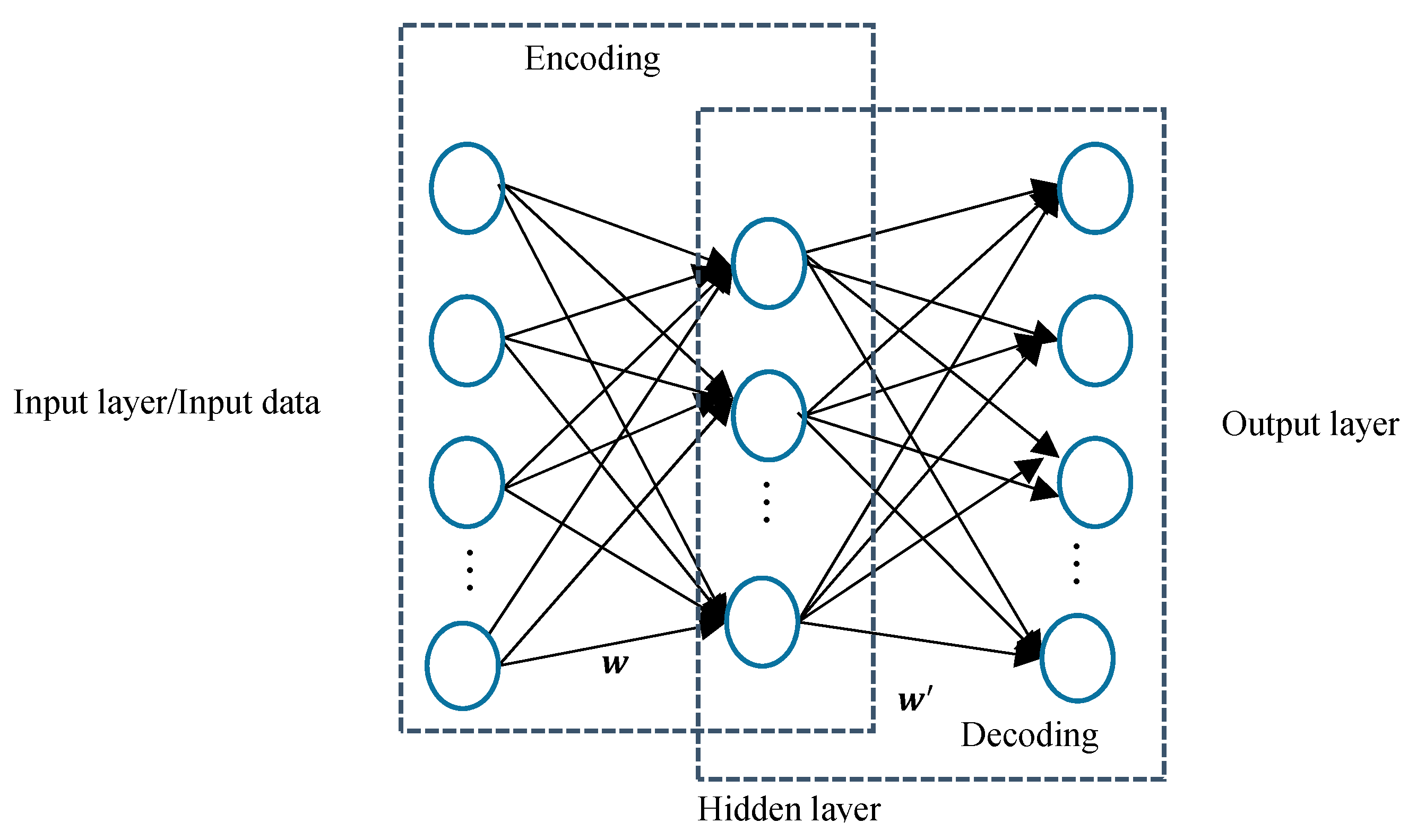
2.2. Autoencoder

The structure of autoencoder is shown in Figure 2. A typical autoencoder contains two parts, namely the encoding and decoding part. As shown in Figure 2, the encoding part maps the input data to the latent expression in the hidden layer, and then the decoding part reconstructed the latent expression to the original data as output. In an autoencoder, all the neurons in the input layer are connected to all the neurons in the hidden layer, and vice versa. With a given input data (bias term included) vector $\mathit{x}$, the latent expression in the hidden layer $h$ can be written as:

$$h=f_e\left(\mathit{w}\mathit{x}\right)$$

(4)

where $\mathit{w}$ represents the weights matrix between each neuron in the input layer and the one in the hidden layer, $f_e$ the non-linear activation function used to smooth the output of the hidden layer. Commonly, the activation function is selected as sigmoid or tanh function.

The decoding portion reverse the maps the latent expression to the data space as:

$$\widehat{\mathit{x}}=f_d\left[{\mathit{w}}^{\prime }{f}_e\left(\mathit{w}\mathit{x}\right)\right]$$

(5)

where $\widehat{\mathit{x}}$ represents the reconstructed data mapped from the latent expression in the hidden layer, ${\mathit{w}}^{\prime }={\mathit{w}}^T$ the weight matrix between hidden layer and the output layer, and $f_d$ the activation function to smooth the output layer results. Likewise, $f_d$ is usually selected as sigmoid or tanh function.

The objective in the autoencoder training procedure is to obtain the set of encoding weights $\mathit{w}$ and decoding weights ${\mathit{w}}^{\prime }$ such that the error between the original input data and the reconstructed data is minimized. The learning objective can be written as:

$$\arg \underset{\mathit{w},{\mathit{w}}^{\prime }}{\min }{\Vert \mathit{x}-\widehat{\mathit{x}}\Vert }_2^2$$

(6)

The smooth and continuously differentiable activation function in the Equation (5) guarantees that even as a non-convex problem in Equation (6), the smooth results leads it can be solved by gradient descent techniques.

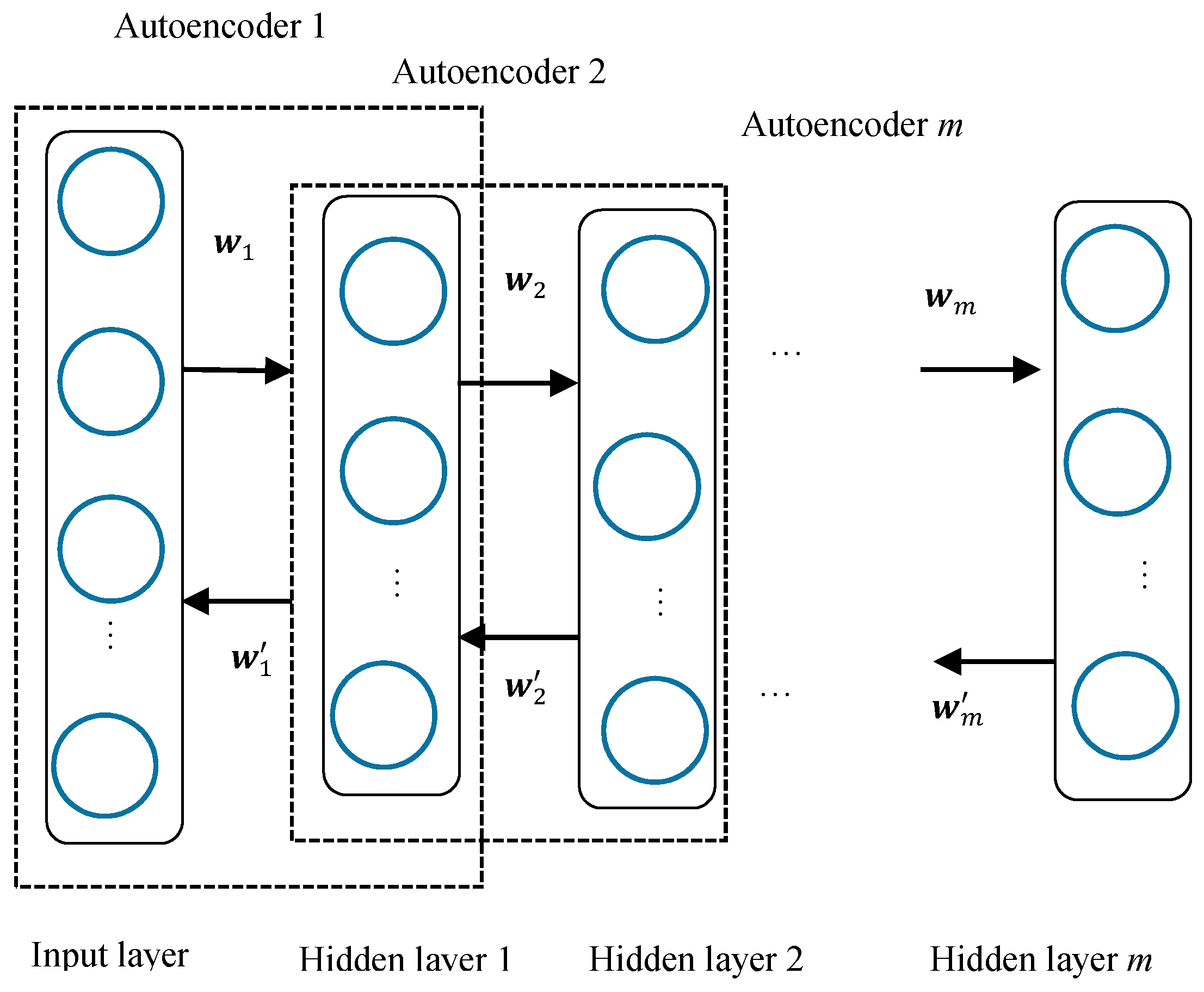
Furthermore, multiple autoencoders can be stacked to construct a deep structure. The deep autoencoder structure is illustrated in Figure 3.

For the deep autoencoders shown in Figure 3, the overall cost function can be expressed based on Equation (6) as: $\underset{{\mathit{w}}_1,\dots ,{\mathit{w}}_{m-1},{\mathit{w}}_1^{\prime },\dots ,{\mathit{w}}_m^{\prime }}{\min }{\Vert \mathit{x}-\widehat{\mathit{x}}\Vert }_2^2$ where $\widehat{\mathit{x}}=f_{d1}{\mathit{w}}_1^{\prime }\left\{{\mathit{w}}_2^{\prime }\dots {\mathit{w}}_m^{\prime }\left[E\left(\mathit{x}\right)\right]\right\}$, and

$$E\left(\mathit{x}\right)=f_{e\left(m-1\right)}\left\{{\mathit{w}}_{m-1}{f}_{e\left(m-2\right)}\left[{\mathit{w}}_{m-2}\dots f_{e1}\left({\mathit{w}}_1\mathit{x}\right)\right]\right\}$$

(7)

where ${\mathit{w}}_i$ and ${\mathit{w}}_i^{\prime }$ ($i=1,2,\dots ,m$) represent the encoding and decoding weight matrix of the i^th autoencoder in the network respectively, $f_{ei}$ and $f_{di}$ the encoding and decoding activation function of the i^th autoencoder. The computational complexity of massive amount of parameters (weight matrix) in Equation (7) results in computation challenge and over fitting phenomena. Thus, searching for the appropriate solution is commonly accomplished through the layer-wise learning behavior.

2.3. Dictionary Learning Using Deep Sparse Autoencoder

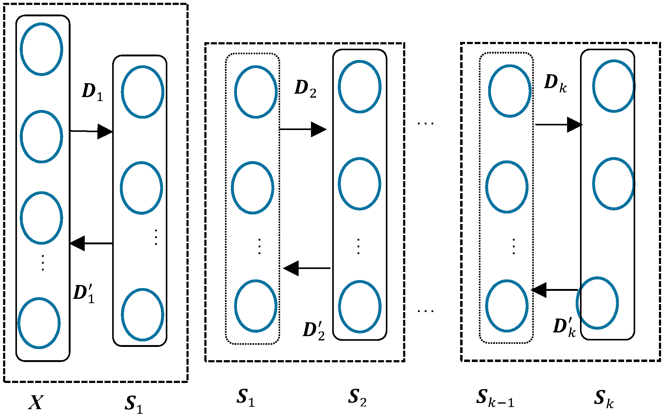
Based on the previously reviewed dictionary learning and stacked autoencoder models, a deep sparse autoencoder based dictionary learning is presented in this section. Like the structure of a deep autoencoder, the deep sparse autoencoder based dictionary learning can be illustrated as Figure 4 below.

As shown in Figure 4, each dash block represents a shallow/single dictionary learning process.

The first dictionary learning process can be written as:

$$\mathit{X}={\mathit{D}}_1{\mathit{S}}_1$$

(8)

where $\mathit{X}={\left\{{\mathit{x}}_i\in {ℝ}^d\right\}}_{i=1}^N$ stands for the set of $N$ input signals,${\mathit{x}}_i$ the signal vector with a length of$d$, ${\mathit{D}}_1=\left\{{\mathit{d}}_1^1,{\mathit{d}}_1^2,\dots ,{\mathit{d}}_1^j,\dots ,{\mathit{d}}_1^K\right\}$ for ${\mathit{d}}_1^j\in {ℝ}^d$ the first learnt dictionary, and ${\mathit{S}}_1=\left\{{\mathit{s}}_1^1,{\mathit{s}}_1^2,\dots ,{\mathit{s}}_1^g,\dots ,{\mathit{s}}_1^N\right\}$ for ${\mathit{s}}_1^g\in {ℝ}^K$ the first latent expression of $\mathit{X}$ in ${\mathit{D}}_1$. Treating the deep autoencoder as a dictionary learning network, one can define ${\mathit{D}}_1^{\prime }=\left\{{{\mathit{d}}^{\prime }}_1^1,{{\mathit{d}}^{\prime }}_1^2,\dots ,{{\mathit{d}}^{\prime }}_1^p,\dots ,{{\mathit{d}}^{\prime }}_1^K\right\}$ for ${{\mathit{d}}^{\prime }}_1^p\in {ℝ}^d$as the reconstruction weight from latent expression ${\mathit{S}}_1$ to original input $\mathit{X}$. Like the expression in the autoencoder, the reconstructed input data $\widehat{\mathit{X}}$ can be written as:

$$\widehat{\mathit{X}}=f_d\left[{\mathit{D}}_1^{\prime }{f}_e({\mathit{S}}_1)\right]$$

(9)

where $f_e$ and $f_d$ represent the encoding and decoding activation functions, respectively.

Substitute ${\mathit{S}}_1$ in Equation (9) with Equation (8), $\widehat{\mathit{X}}$ can be written as:

$$\widehat{\mathit{X}}=f_d\left\{\left[{\mathit{D}}_1^{\prime }{f}_e\left({\mathit{D}}_1^{-1}\mathit{X}\right)\right]\right\}$$

(10)

Here in this study, the activation function for both encoding and decoding processes are selected as sigmoid function. The cost function of dictionary learning using deep sparse autoencoder can be expressed as:

$$\underset{D,D^{\prime }}{\min }\frac{1}{2N}{\Vert \mathit{X}-\widehat{\mathit{X}}\Vert }_2^2+\beta {\displaystyle \sum }_{j=1}^{J}KL(\rho ||{\widehat{\rho }}_j)$$

(11)

$$KL(\rho ||{\widehat{\rho }}_j)=\rho \log \frac{\rho }{{\widehat{\rho }}_j}+\left(1-\rho \right)\log \frac{1-\rho }{1-{\widehat{\rho }}_j}$$

(12)

$$\widehat{{\rho }_j}=\frac{1}{N}{\left[1+\exp \left(-{\mathit{D}}^{-1}\mathit{X}\right)\right]}^{-1}$$

(13)

where N represents the number of input vectors, $\beta$ the parameter controlling the weight of the sparsity penalty term, $\rho$ the sparsity parameter, ${\widehat{\rho }}_j$ the average activation of the hidden unit $j$ over the all $N$ training samples. The sparsity penalty term is defined as Kullback-Leibler (KL) divergence, which is used to measure the difference between two distributions. It is defined as $KL(\rho |\left|\widehat{{\rho }_j}\right)=0$ when $\rho ={\rho }_j$, otherwise the KL divergence increases as $\left|\rho -{\rho }_j\right|$ increases. In comparison with the similar k-sparse autoencoder proposed in [30], the advantages of the deep sparse autoencoder include: (1) The introduction of the sparsity penalty leads to the automatic determination of the sparsity rather than pre-defined as k-sparsity. It enables the deep sparse autoencoder to extract the sparse features more accurately based on the characteristics of the data. (2) The dictionary is learnt in the encoding procedure. The encoding dictionary is different from the encoding weight matrix. (3) The deep sparse autoencoders does not require the fine-tuning process while the performance of k-sparse autoencoders relies on the supervised fine-tuning process.

In the deep autoencoder, the output of a hidden layer in the previous autoencoder can be taken as the input to the next autoencoder. Let the first layer of the k^th autoencoder in the deep autoencoder be the k^th layer and the second layer as the (k + 1)^th layer. Also, let ${\mathit{D}}_k$ and ${\mathit{D}}_k^{\prime }$ be the dictionary and reconstruction weight for the k^th layer in the deep autoencoder, the encoding procedure in the k^th autoencoder can be expressed as:

$${\mathit{a}}^k=f_e\left({\mathit{z}}^k\right)$$

(14)

$${\mathit{z}}^{k+1}={{\mathit{D}}_k}^{-1}{\mathit{a}}^k$$

(15)

where ${\mathit{a}}^k$ stands for the output of the k^th layer, ${\mathit{z}}^k$ and ${\mathit{z}}^{k+1}$ the input for the k^th and (k + 1)^th layer, respectively.

Similarly, the decoding procedure in the k^th autoencoder can be expressed as:

$${\mathit{a}}^k=f_d\left({\mathit{z}}^k\right)$$

(16)

$${\mathit{z}}^{k-1}={{\mathit{D}}_k}^{\prime }{\mathit{a}}^k$$

(17)

Thus, the original input $\mathit{X}$ can be expressed by the latent expression $S_k$ in the (k + 1)^th layer as:

$$\mathit{X}=({\mathit{D}}_1{\mathit{D}}_2\dots {\mathit{D}}_k)S_k$$

(18)

where ${\mathit{D}}_k$ represents the learnt dictionary in the k^th dictionary learning process, $S_k$ the latent expression of $\mathit{X}$ in ${\mathit{D}}_k$.

The stacked dictionaries $\left({\mathit{D}}_1{\mathit{D}}_2\dots {\mathit{D}}_k\right)$ will be learnt in a greedy layer by layer way. The greedy layer by layer learning guarantees the convergence at each layer.

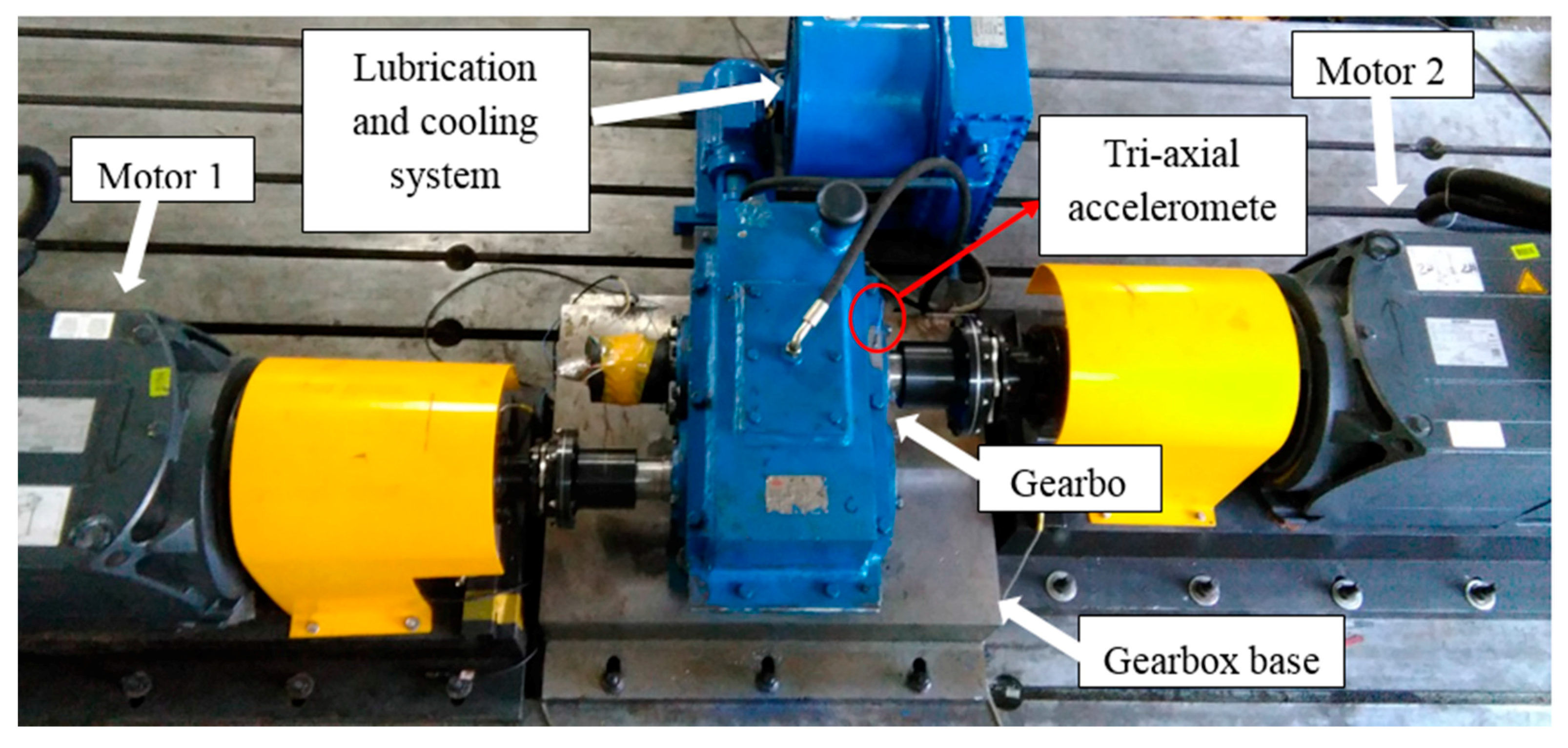
3. Gear Test Experimental Setup and Data Collection

The gear pitting tests were performed on a single stage gearbox installed as an electronically closed transmission test rig. The gearbox test rig includes two 45 kW Siemens servo motors. One of the motors can act as the driving motor while the other can be configured as the load motor. The configuration of the driving mode is flexible. Compared with traditional open loop test rig, the electrically closed test rig is economically more efficient, and can virtually be configured with arbitrary load and speed specifications within the rated power. The overall gearbox test rig, excluding the control system, is showed in Figure 5.

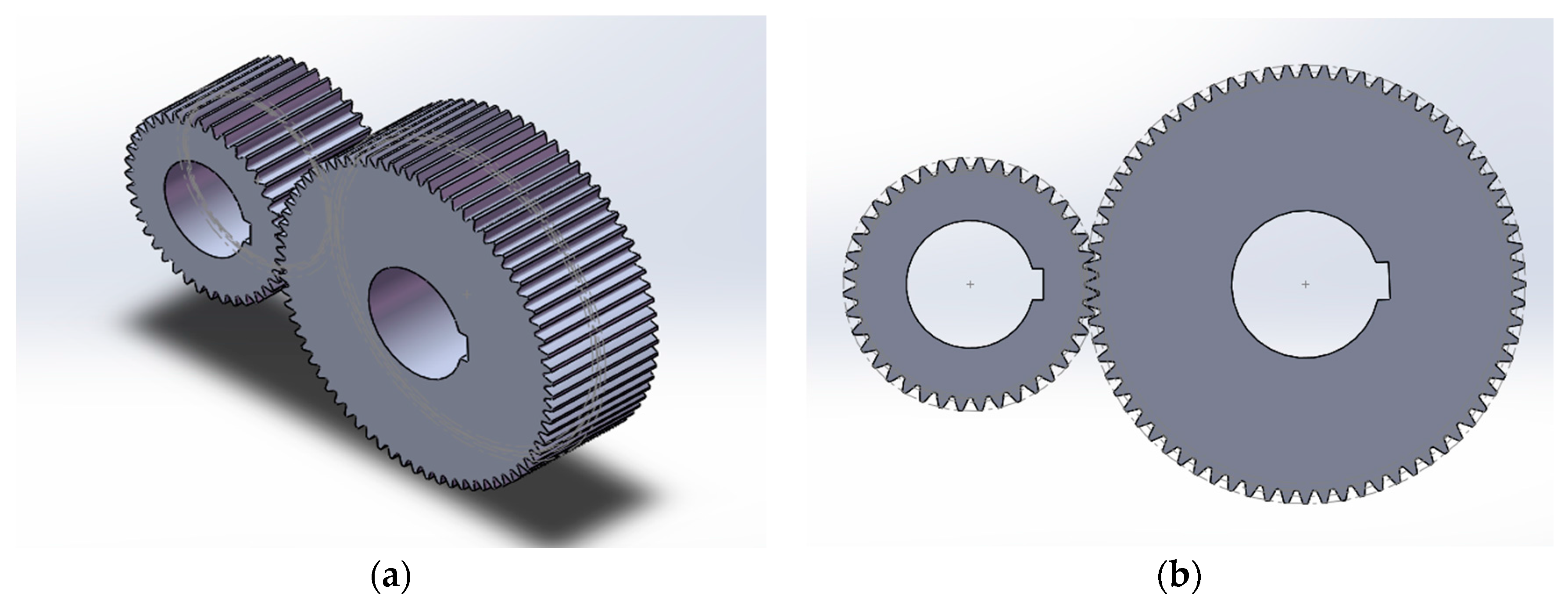
The testing gearbox is a single stage gearbox with spur gears. The gearbox has a speed reduction of 1.8:1. The input driving gear has 40 teeth and the driven gear has 72 teeth. The 3-D geometric model of the gearbox is shown in Figure 6.

Gear parameters are provided in

Table 1. List of gear parameters for the tested gearbox.

Gear Parameter	Driving Gear	Driven Gear
Tooth number	40	72
Module	3 mm	3 mm
Base circle diameter	112.763 mm	202.974 mm
Pitch diameter	120 mm	216 mm
Pressure angle	20°	20°
Addendum coefficient	1	1
Coefficient of top clearance	0.25	0.25
Diametric pitch	8.4667	8.4667
Engaged angle	19.7828°	19.7828°
Circular pitch	9.42478 mm	9.42478 mm
Addendum	4.5 mm	3.588 mm
Dedendum	2.25 mm	3.162 mm
Addendum modification coefficient	0.5	0.196
Addendum modification	1.5 mm	0.588 mm
Fillet radius	0.9 mm	0.9 mm
Tooth thickness	5.8043 mm	5.1404 mm
Tooth width	85 mm	85 mm
Theoretical center distance	168 mm	168 mm
Actual center distance	170.002 mm	170.002 mm

.

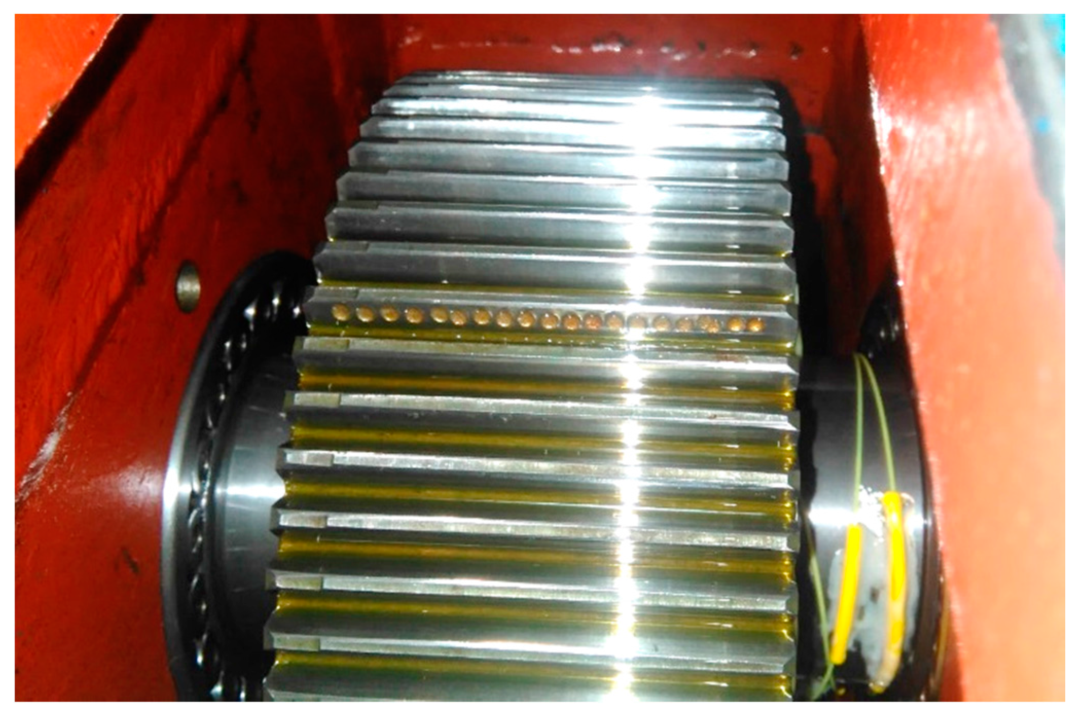
The pitting fault was simulated by using electrical discharge machine to erode gear tooth face. The pitting location is on one of the teeth on the output driven gear with 72 teeth. Approximately, the gear tooth face was eroded with a depth of 0.5 mm. One row of pitting faults was created along the tooth width. The simulated pitting fault is shown in Figure 7.

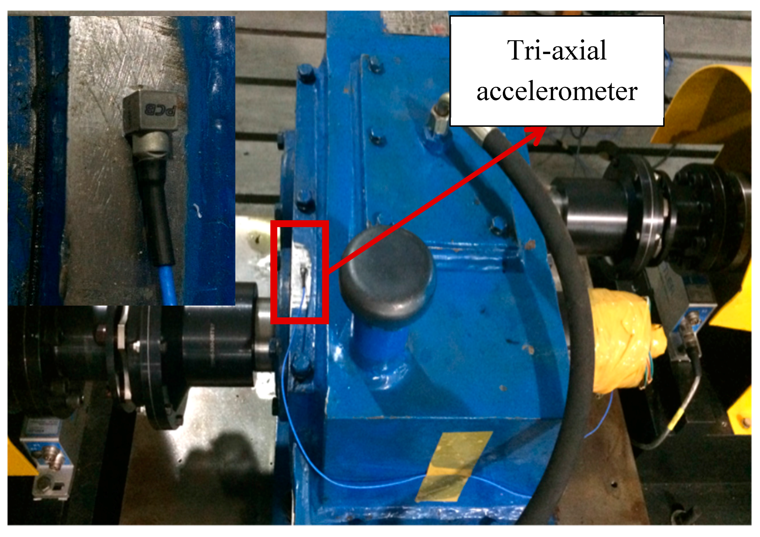
A tri-axial accelerometer was attached on the gearbox case close to the bearing house on the output end as shown in Figure 8.

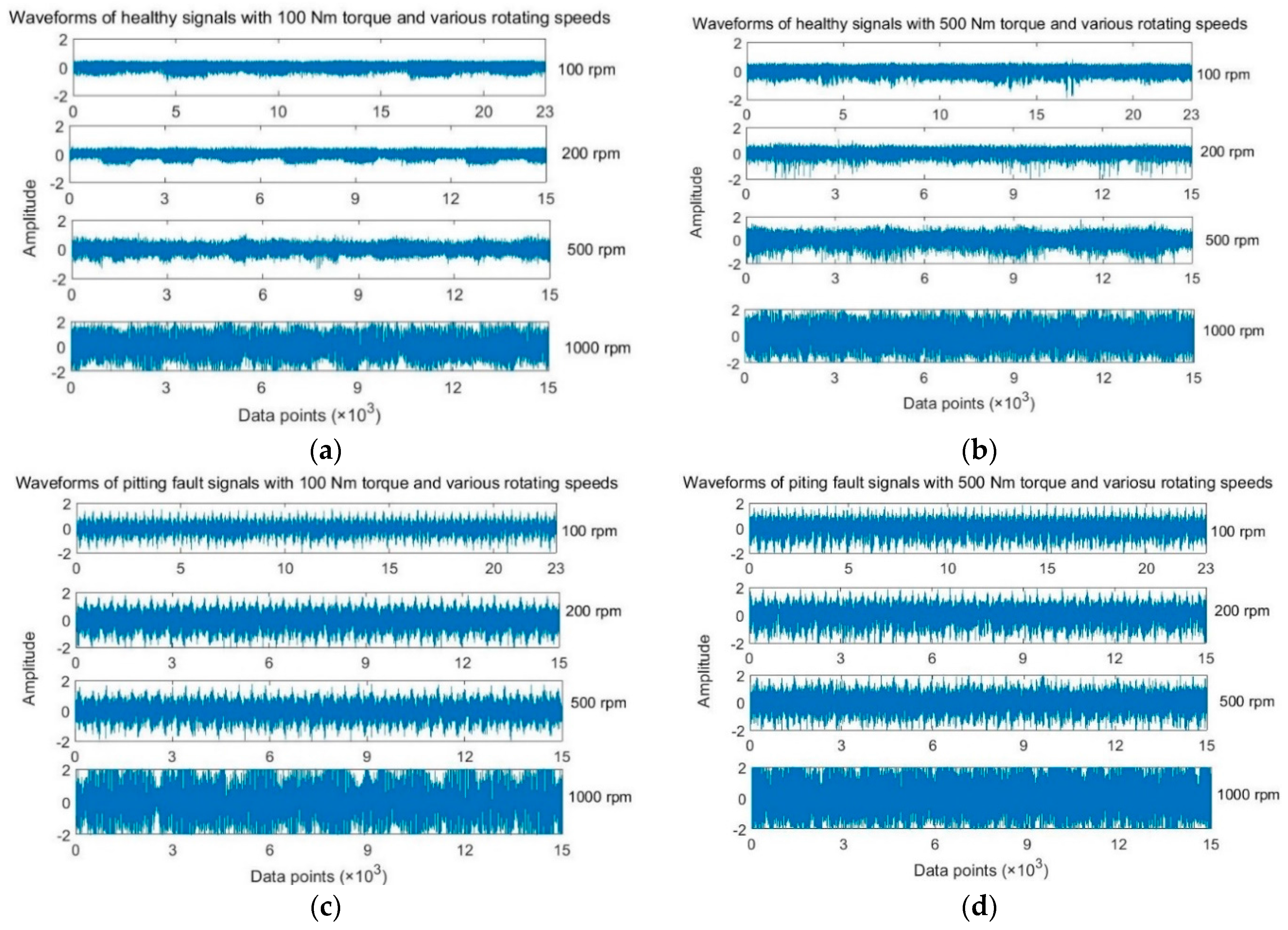
Both healthy and pitted gearboxes under various operating condition were run and the vibration signals collected. The tested operation conditions are listed in

Table 2. Operation condition of the experiments.

Speed (rpm)	100	200	500	1000
Torque (Nm)	50/100/200/300/400/500	50/100/200/300/400/500	50/100/200/300/400/500	50/100/200/300/400/500

. The vibration signals were collected with a sampling rate of 20.48 KHz.

Figure 9 shows the raw vibration signals collected for normal gear and pitting gear at loading conditions of 100 Nm and 500 Nm.

4. The Validation Results

The proposed deep sparse autoencoder structure was implemented to accomplish the greedy deep dictionary learning. The vibration signals along the z vertical direction were used in this study since they contain the richest vibration information among the three monitored directions. At first, the gear pitting detection was carried on using signals with light loading as the training data and signals with heavy loadings as the testing data, respectively. Loadings of 100 Nm torque and 500 Nm torque were used as light loading condition and heavy loading condition, respectively. Signals at rotating speeds of 100, 200, 500 and 1000 rpm were used for validation tests. To study the influence of different rotating speeds on the pitting gear fault detection performance of the deep sparse autoencoder, 100 and 1000 rpm were selected as low and high speed for independent validations. The length of the samples was decided to ensure that at least one revolution of the output driven gear was included. Therefore, there were 23,000 data points in each sample for signals at 100 rpm and 15,000 data points for signals at a speed of at least 200 rpm. Thus, 26 samples of signals at 100 rpm were generated for healthy gear and pitting gear, respectively. Hence, there were 52 samples in the training dataset and 52 samples in the testing dataset. Similarly, 40 samples of signals at 1000 rpm were generated for each gear condition, with 80 samples in the training dataset and 80 samples in the testing dataset. The structure of the deep sparse autoencoder was designed separately for signals at 100 rpm and signals at the speed of over 100 rpm as: one input layer (23,000 neurons for signals at 100 rpm and 15,000 neurons for signals at the speed over 100 rpm), four hidden layers (1000-500-200-50 neurons), and one output layer (2 neurons). Particularly, following the suggestions in [31], the sparsity parameter in each sparse autoencoder was set as $\beta$= 3 and $\rho =0.005$. The sparse representations of the original signals were imported into classifier for pitting gear fault detection. The last hidden layers of 50 neurons and the output layer of 2 neurons were constructed as a simple backpropagation neural network as a classifier for gear pitting detection. The two neurons in the output layer were setup for classifying the input signals as either gear pitting fault or normal gear. The training parameters of the back propagation neural network classifier were set as: training epoch was 100, learning rate was 0.05 and the momentum was 0.05. For each gear condition, the models were executed 5 times to get average detection accuracy. The detection results are shown in

Table 3. Detection results at 100 and 1000 rpm (trained with light loading samples and tested with heavy loading samples).

Gear Conditions	Training Accuracy (100 Nm) (100 rpm/1000 rpm)	Testing Accuracy (500 Nm) (100 rpm/1000 rpm)
Healthy gear	100%/99.50%	99.23%/98.84%
Pitting gear	98.43%/100%	98.43%/98.91%
Overall accuracy	99.22%/99.75%	98.83%/98.88%

.

The detection results in Table 3 show a good adaptive learning performance of the presented method. The testing accuracy is high as 98.88% overall, which is slightly lower than the training accuracy. It can be explained as that signals at light loading condition contain less fault significant information. Furthermore, the same designed deep sparse autoencoder structure was experimented with heavy loading training data and light loading testing data. The detection results are shown in

Table 4. Detection results at 100 and 1000 rpm (trained with heavy loading samples and tested with light loading samples).

Gear Conditions	Training Accuracy (500 Nm) (100 rpm/1000 rpm)	Testing Accuracy (100 Nm) (100 rpm/1000 rpm)
Healthy gear	100%/99.95%	100%/99.90%
Pitting gear	100%/100%	99.23%/100%
Overall accuracy	100%/99.98%	99.62%/99.95%

.

It can be observed from Table 4 that in comparison with results shown in Table 3, the testing accuracy is slightly higher than the training accuracy. The better adaptive feature extraction and fault detection results are benefited from that the signals with heavy loading condition contain more fault significant information. The results in Table 3 and Table 4 show marginal influence of the rotating shaft speeds on the pitting fault detection performance.

Moreover, the signals with stable loading and mixed rotating speed were also tested in the study. The detailed description of each dataset used in the validation is provided in

Table 5. Dataset description.

Dataset	Loading Condition of the Training Dataset (Nm)	Loading Condition of the Testing Dataset (Nm)	Rotating Speed (rpm)	Length of Signal Sample
A	100	500	100	23,000
B	500	100	100	23,000
C	100	500	1000	15,000
D	500	100	1000	15,000
E	100	500	100/200/500/1000	15,000
F	500	100	100/200/500/1000	15,000

. The detection results are presented in

Table 6. Detection results at mixed rotating speeds (trained with light loading samples and tested with heavy loading samples).

Gear Conditions	Training Accuracy (100 Nm)	Testing Accuracy (500 Nm)
Healthy gear	99.45%	97.21%
Pitting gear	99.65%	97.05%
Overall accuracy	99.55%	97.13%

and

Table 7. Detection results at mixed rotating speeds (trained with heavy loading samples and tested with light loading samples).

Gear Conditions	Training Accuracy (500 Nm)	Testing Accuracy (100 Nm)
Healthy	99.45%	99.94%
Pitting gear	99.58%	99.84%
Over all	99.52%	99.89%

.

Still, 100 and 500 Nm torque loadings were selected as the light loading and heavy loading condition. For each loading condition, 52 samples and 80 samples were generated for both healthy and pitting gear condition at 100 rpm and at the speeds over 100 rpm, respectively. In comparison with the results in Table 3 and Table 4, even though the detection accuracies in Table 6 and Table 7 for both cases (trained with light loading samples and tested with heavy loading samples, and vice versa) are slightly lower, the accuracies obtained by the deep sparse autoencoders are satisfactorily as high as 97.13% and 99.89%. The satisfactory detection results show the good performance without the effects of various rotating speeds of the deep sparse autoencoders. Furthermore, it shows the capability of the deep sparse autoencoders in automatically extracting the adaptive features from the raw vibration signals. The validation results have shown the good robustness of the deep sparse autoencoders on gear pitting detection without much influence of working conditions, including loadings and rotating speeds.

To make a comparison, a typical autoencoder based deep neural network (DNN) presented in [32] was selected to detect the gear pitting fault using the same data. The DNN was designed with a similar structure like the deep sparse autoencoder, namely one input layer (23,000 neurons and 15,000 neurons), four hidden layers (1000-500-200-50 neurons), and one output layer (2 neurons). Like the deep sparse autoencoder, the last hidden layer and the output layer of the DNN was designed as a back propagation neural network classifier. Since the autoencoder based neural network normally requires supervised fine-tuning process for better classification, the designed DNN was tested without and with supervised fine-tuning. The detection results of the DNN are provided in

Table 8. Detection results of DNN at mixed rotating speeds (trained with light loading samples and tested with heavy loading samples).

Gear Conditions	Training Accuracy (100 Nm)		Testing Accuracy (500 Nm)
	Without Supervised Fine-Tuning	With Supervised Fine-Tuning	Without Supervised Fine-Tuning	With Supervised Fine-Tuning
Healthy gear	85.25%	90.50%	83.42%	89.85%
Pitting gear	85.85%	89.95%	81.15%	88.24%
Overall accuracy	85.55%	90.23%	82.29%	89.05%

and

Table 9. Detection results of DNN at mixed rotating speeds (trained with heavy loading samples and tested with light loading samples).

Gear Conditions	Training Accuracy (500 Nm)		Testing Accuracy (100 Nm)
	Without Supervised Fine-Tuning	With Supervised Fine-Tuning	Without Supervised Fine-Tuning	With Supervised Fine-Tuning
Healthy gear	82.18%	90.25%	84.25%	91.50%
Pitting gear	84.15%	88.85%	85.17%	91.50%
Overall accuracy	83.17%	89.55%	84.71%	91.50%

.

In comparing the results obtained by the DNN in Table 8 and Table 9 with those obtained by the deep sparse autoencoder, one can see that the deep sparse autoencoder gives a better performance than the DNN based approach for gear pitting fault detection. In both cases, the detection accuracies obtained by the DNN are much lower than those of the deep sparse autoencoder. In comparison with the DNN, the presented method is more robust in automatically extracting the adaptive features for gear pitting detection. In addition, the presented method does not require the supervised fine-tuning process. Such advantage will increase the computational efficiency and enhance the robustness of the gear pitting fault detection in dealing with massive data.

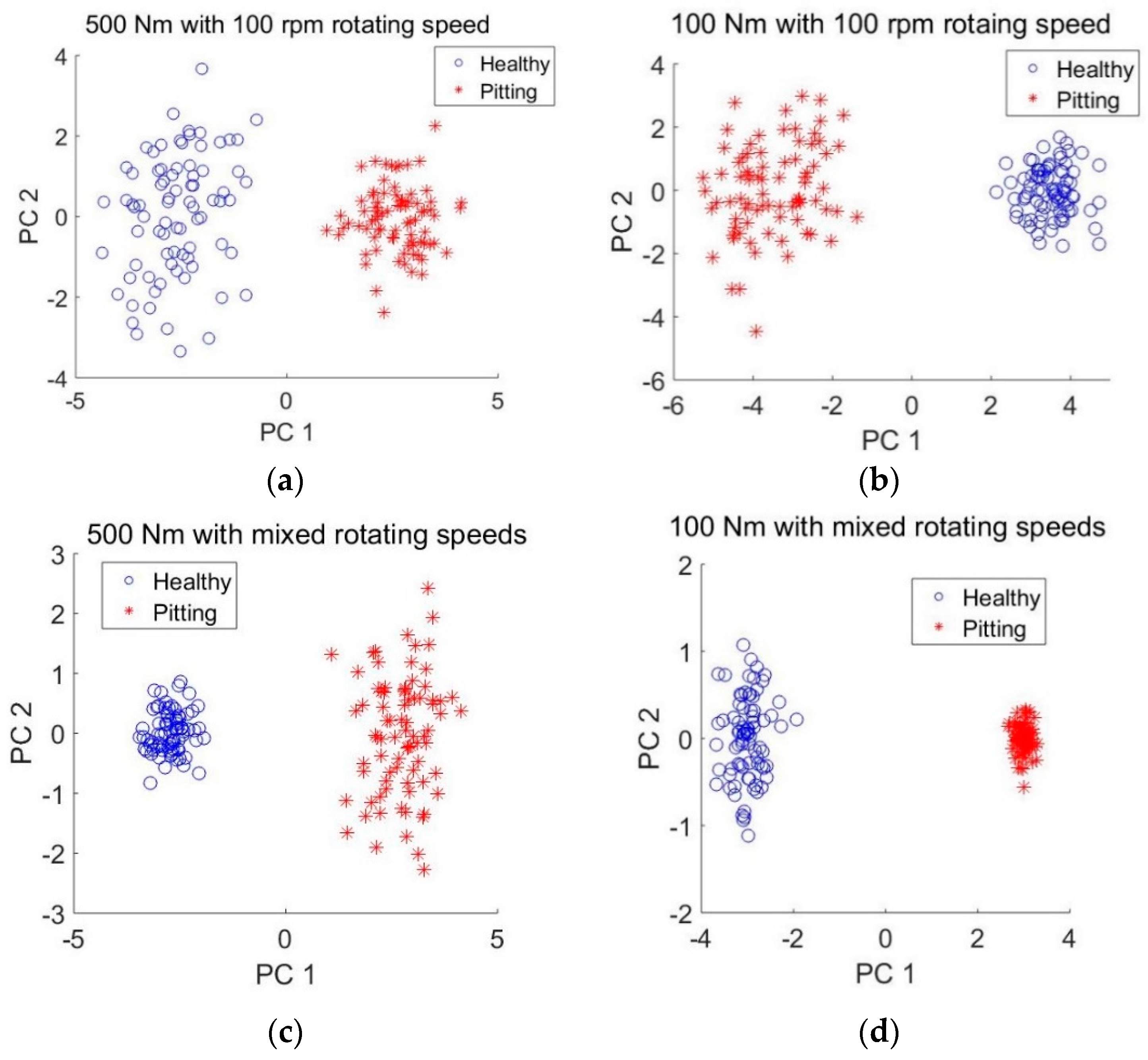
To verify the ability of the presented method for automatically adaptive features extraction, using a similar approach in [33], the principal component analysis (PCA) was employed to visualize the extracted features. The values of neurons in the last hidden layer were regarded as pitting fault features since they were used for pitting detection in the output layer. Therefore, 50 features were obtained by the deep sparse autoencoders. The first two principle components were used for the visualization since they carried out more than 90% information in the feature domain. Since pitting gear detection results at rotating speed of 1000 rpm is slightly more accurate than that at 100 rpm, only features obtained using signals at 100 rpm were plotted for observation. The scatter plot of principle components of the features automatically extracted from datasets A, B, E and F are presented in Figure 10.

It can be observed from Figure 10 that the features of the same health condition are grouped in the corresponding clusters which are clearly separated from each other. In comparison with Figure 10a,c, Figure 10b,d show a better clustering performance and more clear separation boundary between the healthy and pitting gear conditions. This could be due to the fact that the features of heaving loading conditions in A and E are extracted using the deep sparse autoencoders trained with data of light loading conditions. The fault features of light conditions are normally less significant than those of heavy loading conditions.

5. Conclusions

Gears are one of the most critical components in many industrial machines and pitting is one of the most common gear faults and normally difficult to detect. An undetected gear pitting fault during the operation of the gears can lead to catastrophic failures of the machines. In this paper, a new method for gear pitting fault detection was presented. The presented method was developed based on a deep sparse autoencoder that integrates dictionary learning in sparse coding into a stacked autoencoder network. The presented method uses a stacked autoencoder network to perform the dictionary learning in sparse coding and automatically extract features from raw vibration data. These features are then used to train a simple backpropagation neural network to perform pitting fault detection. The presented method was validated with vibration data collected from tests with gear pitting faults in a gearbox test rig and compared with a deep neural network based approach. In the validation tests, data obtained from one loading condition was used to train the gear pitting detection model and the model was then tested with data obtained from a different loading condition. The validation results have shown the good robustness of the deep sparse autoencoders on gear pitting detection without much influence of working conditions, including loadings and rotating speeds. The comparison between the deep sparse autoencoder and the deep neural network has shown the outstanding performance of the presented method on automatically extracting the adaptive features than the deep neural network based method.