
Intent-Estimation- and Motion-Model-Based Collision Avoidance Method for Autonomous Vehicles in Urban Environments


Abstract
:
1. Introduction
2. Intent-Estimation- and Motion-Model-Based Collision Avoidance Method
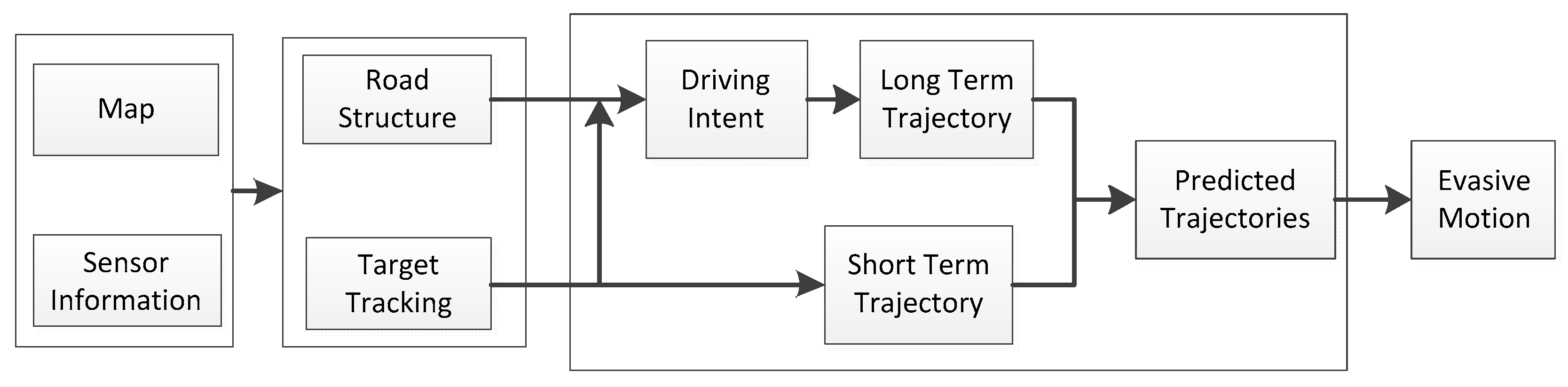
2.1. Overview
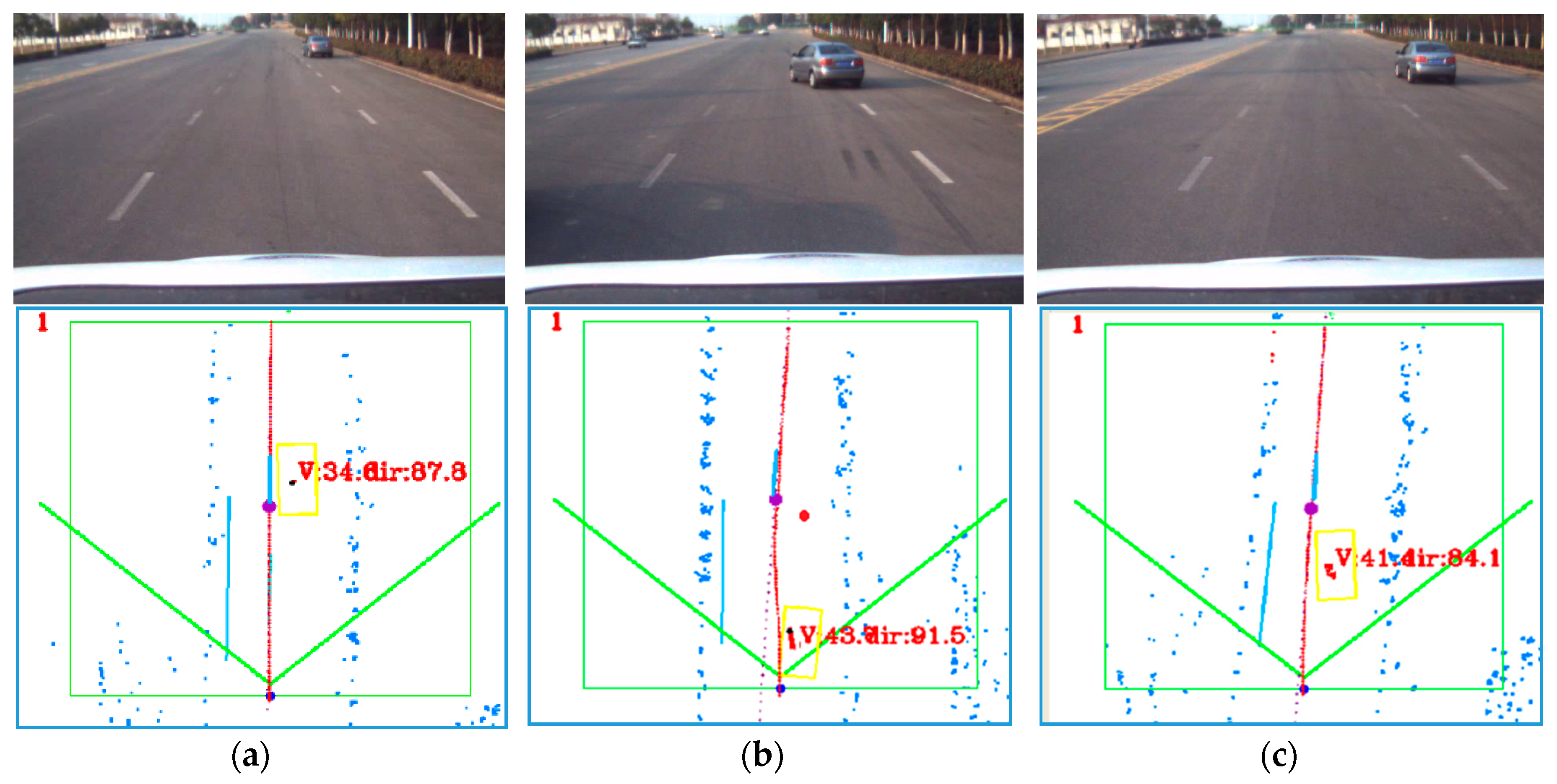
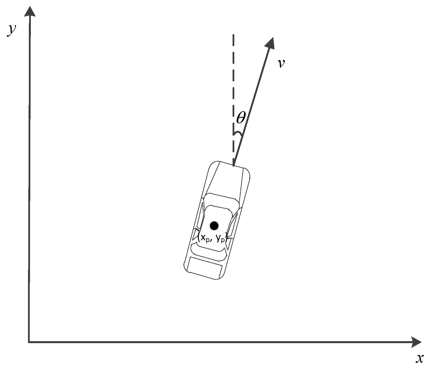
2.2. Intent Estimation
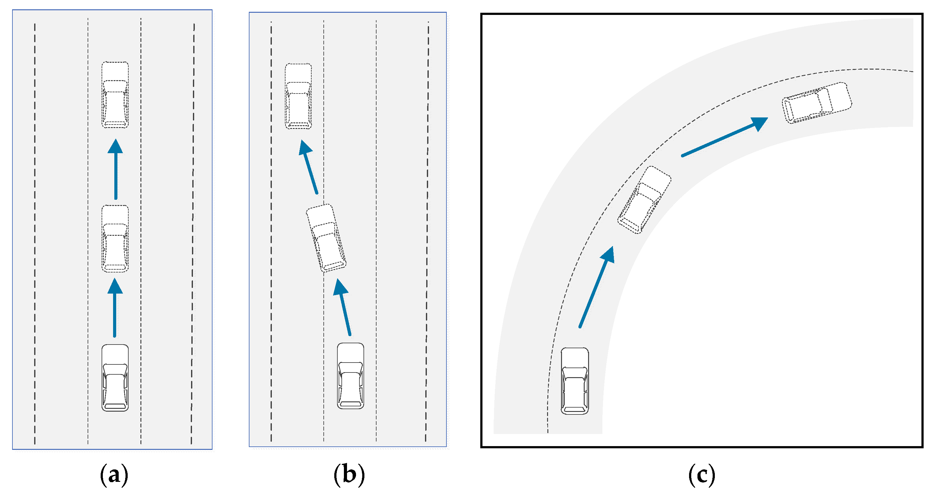
- Normal moving (moving along the lane)
- Left change
- Right lane change
- Turn
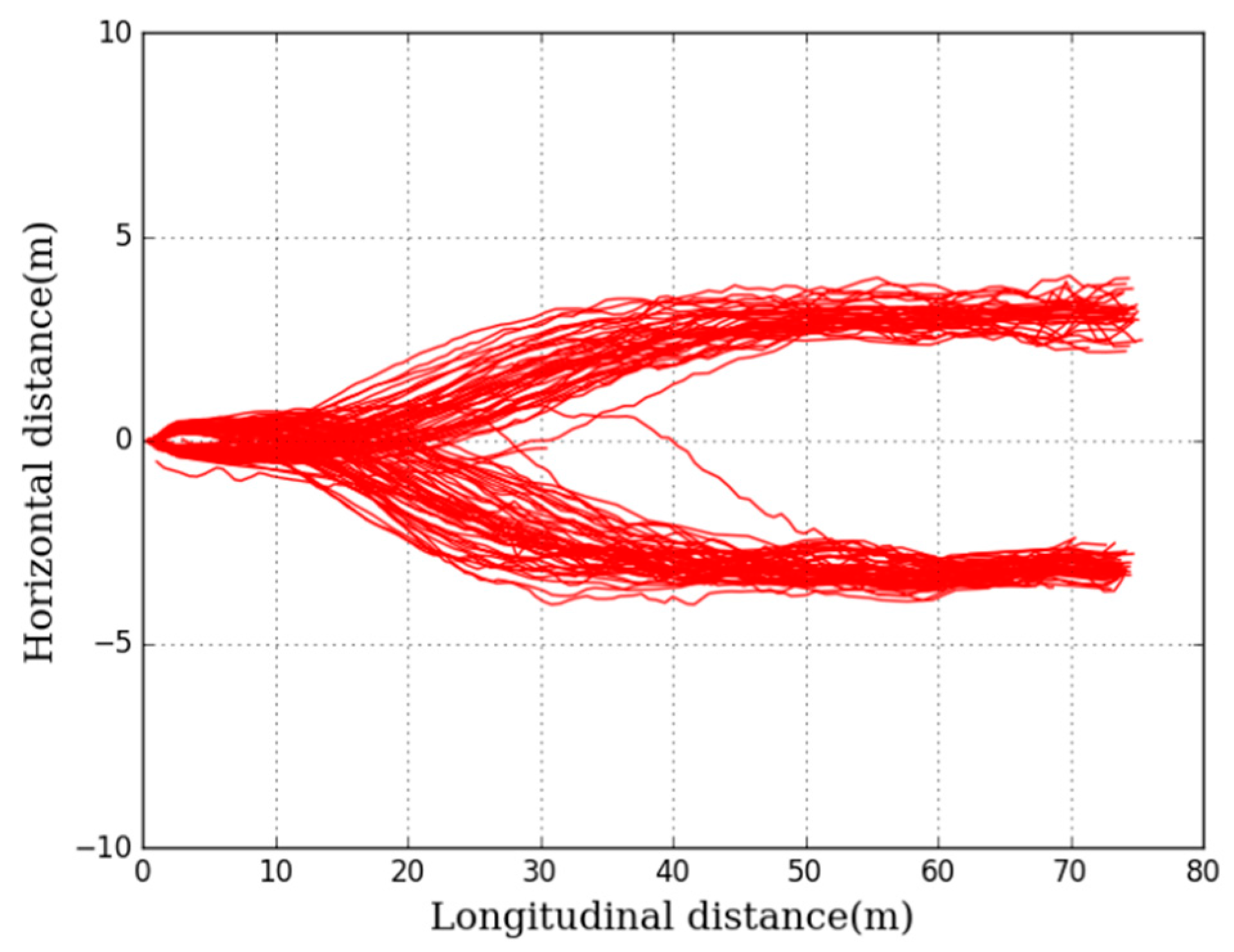
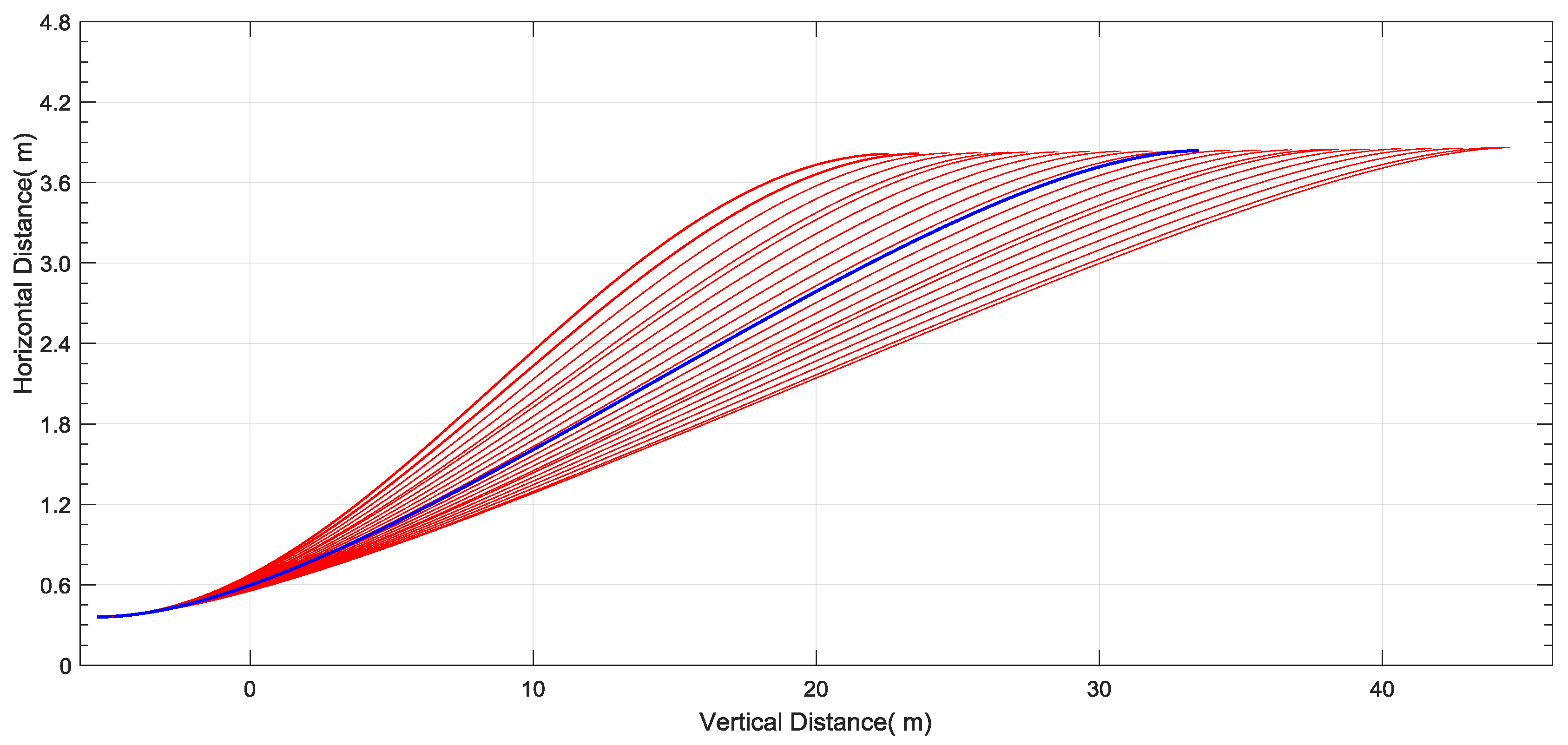
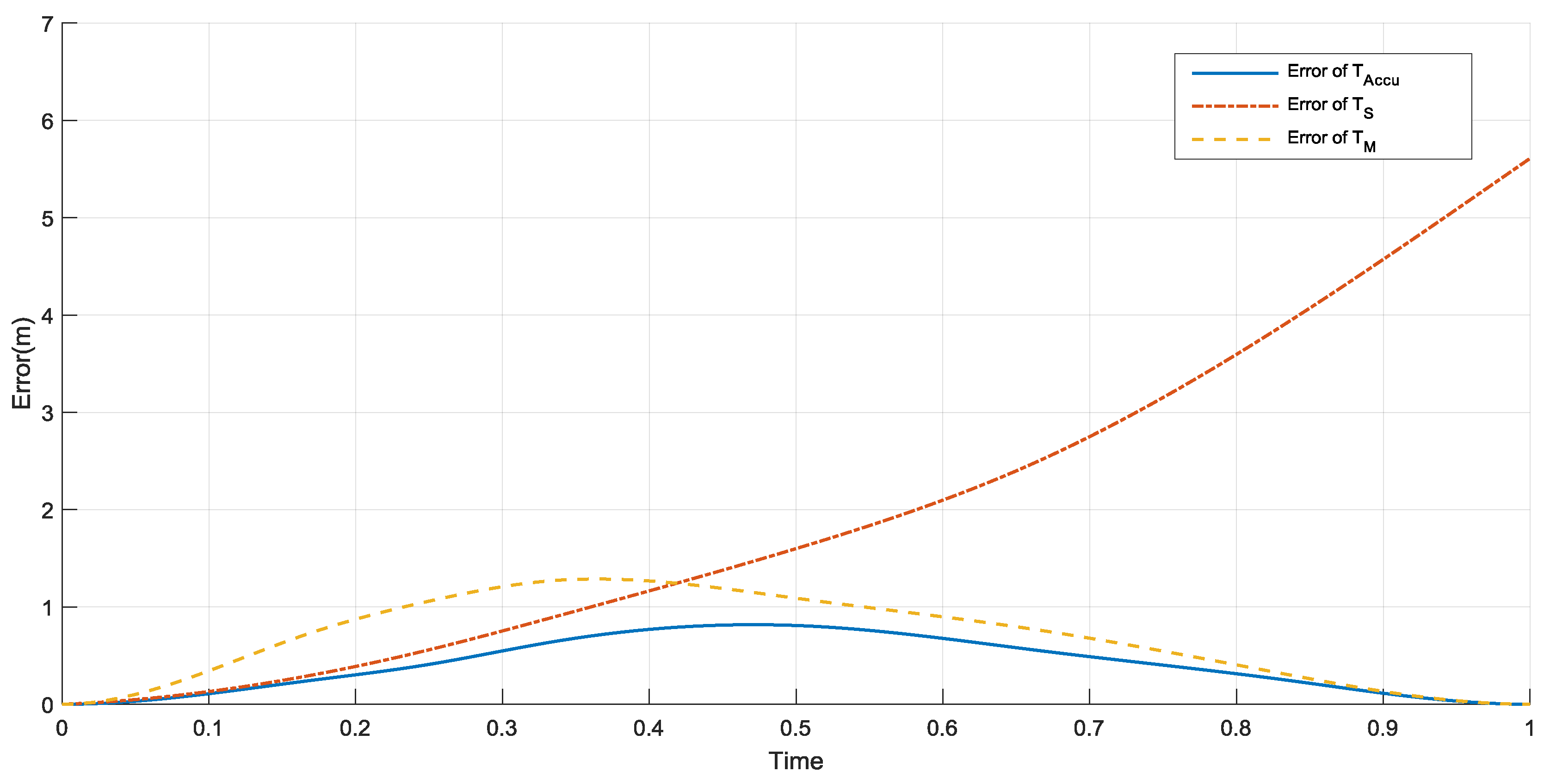
2.3. Trajectory Prediction with Intent and Motion Model
2.4. Collision Avoidance
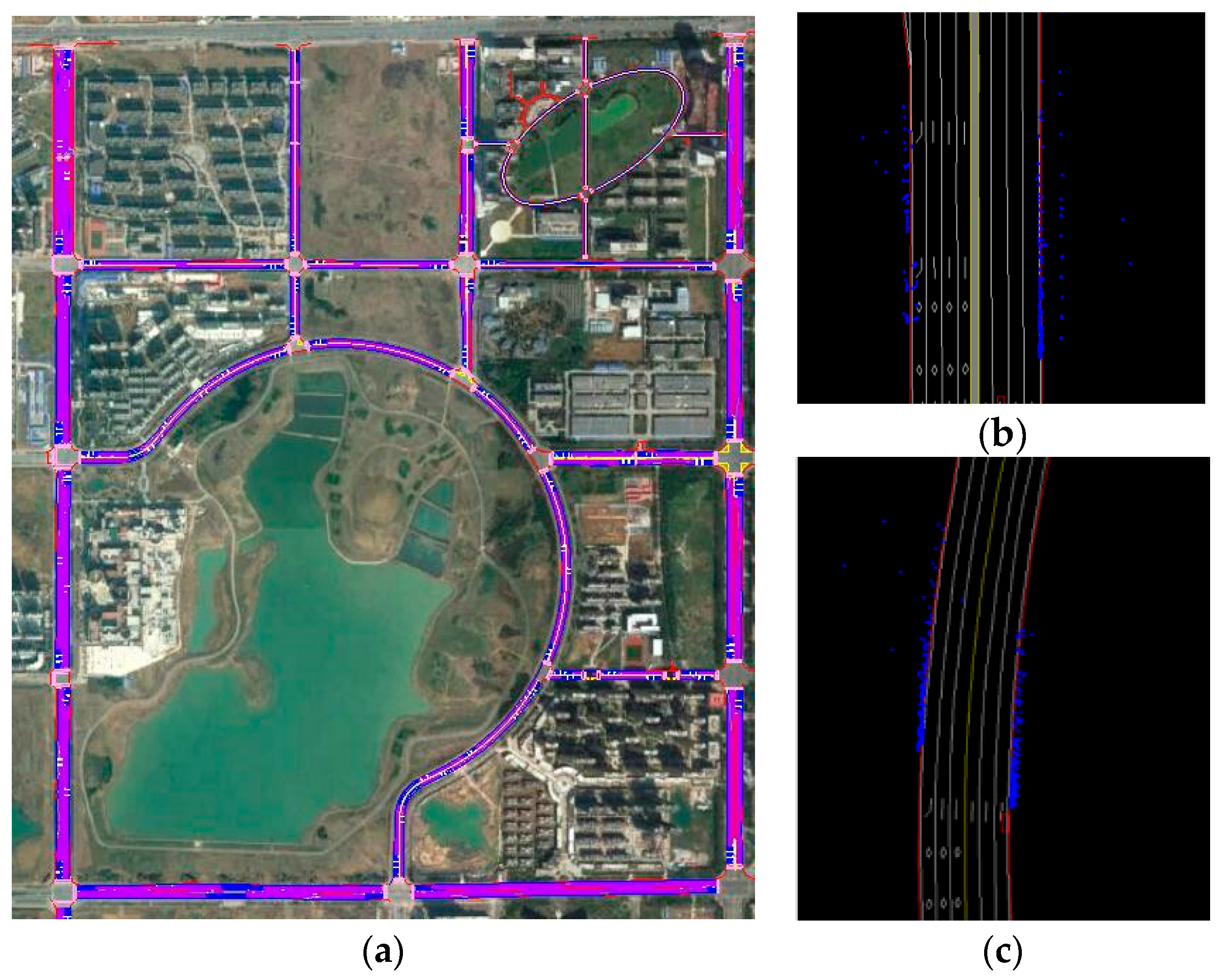
3. Experiments and Discussion
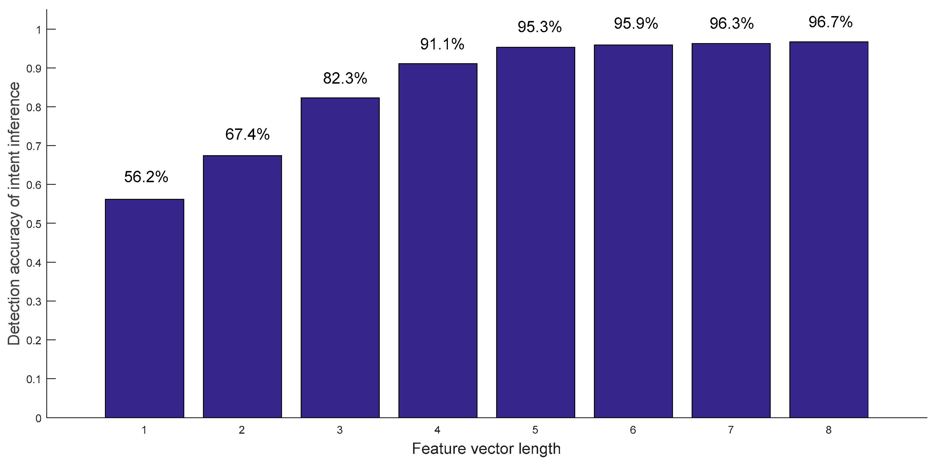
3.1. Performance of the Intent-Estimation Method
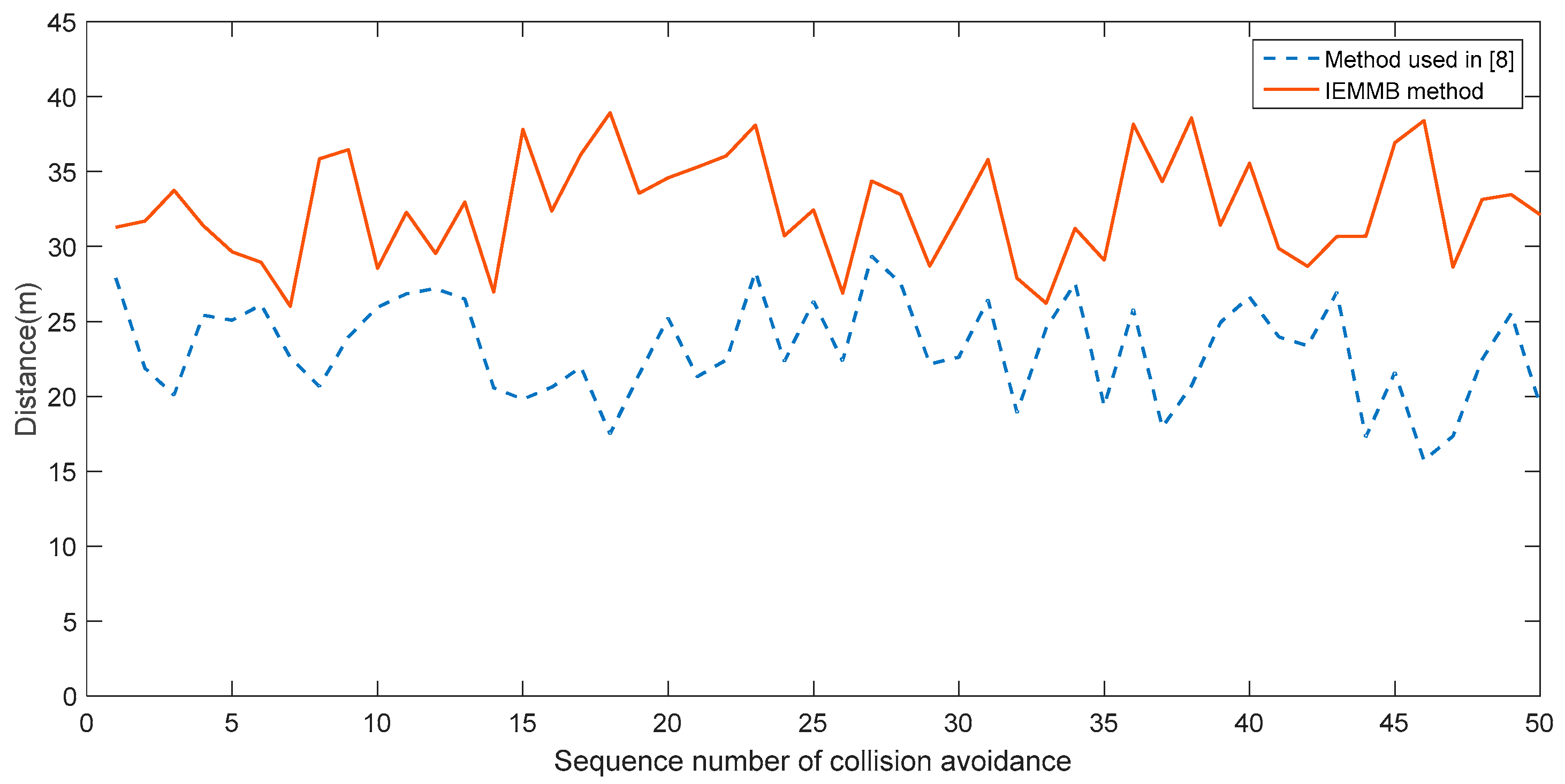
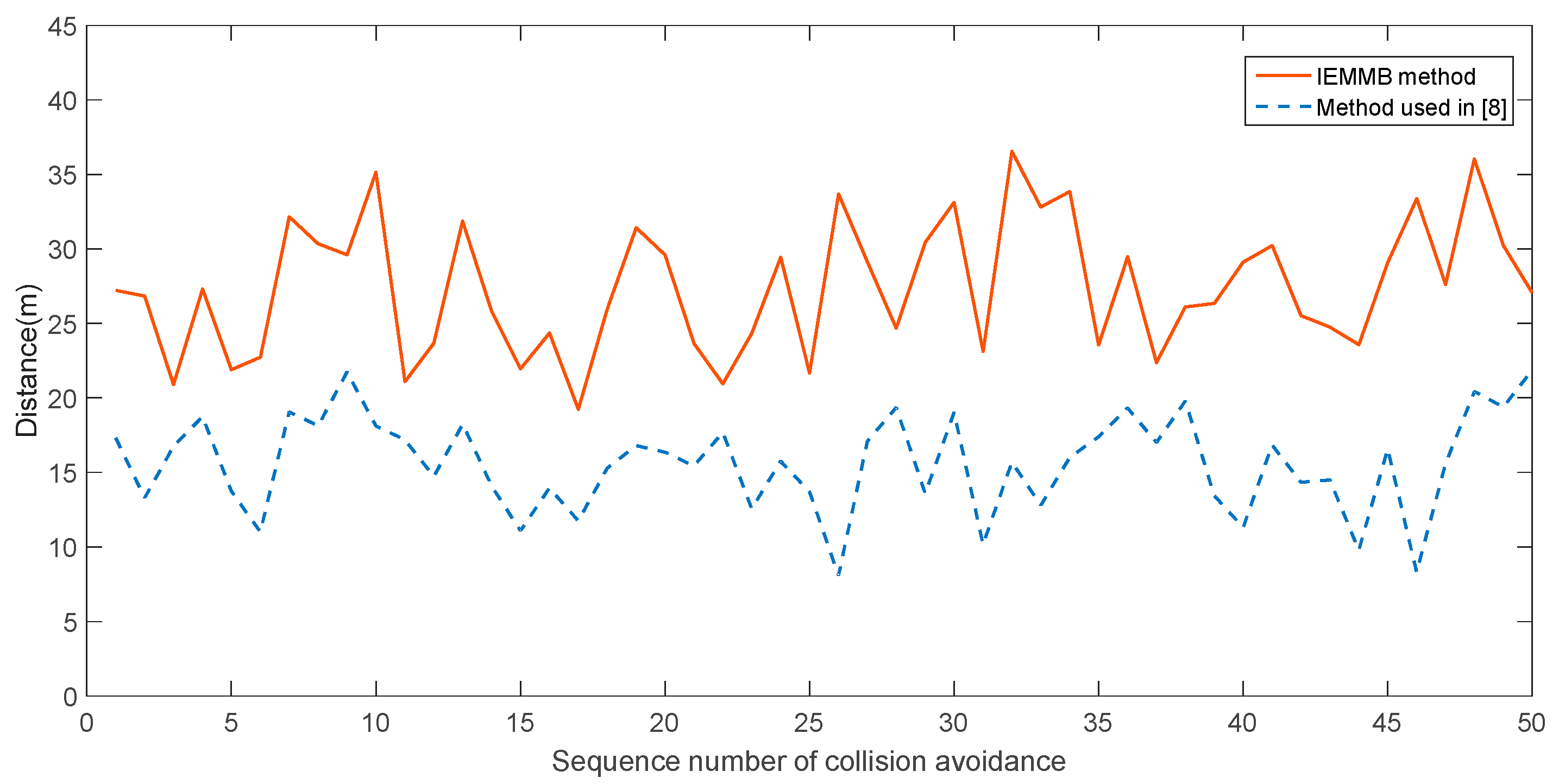
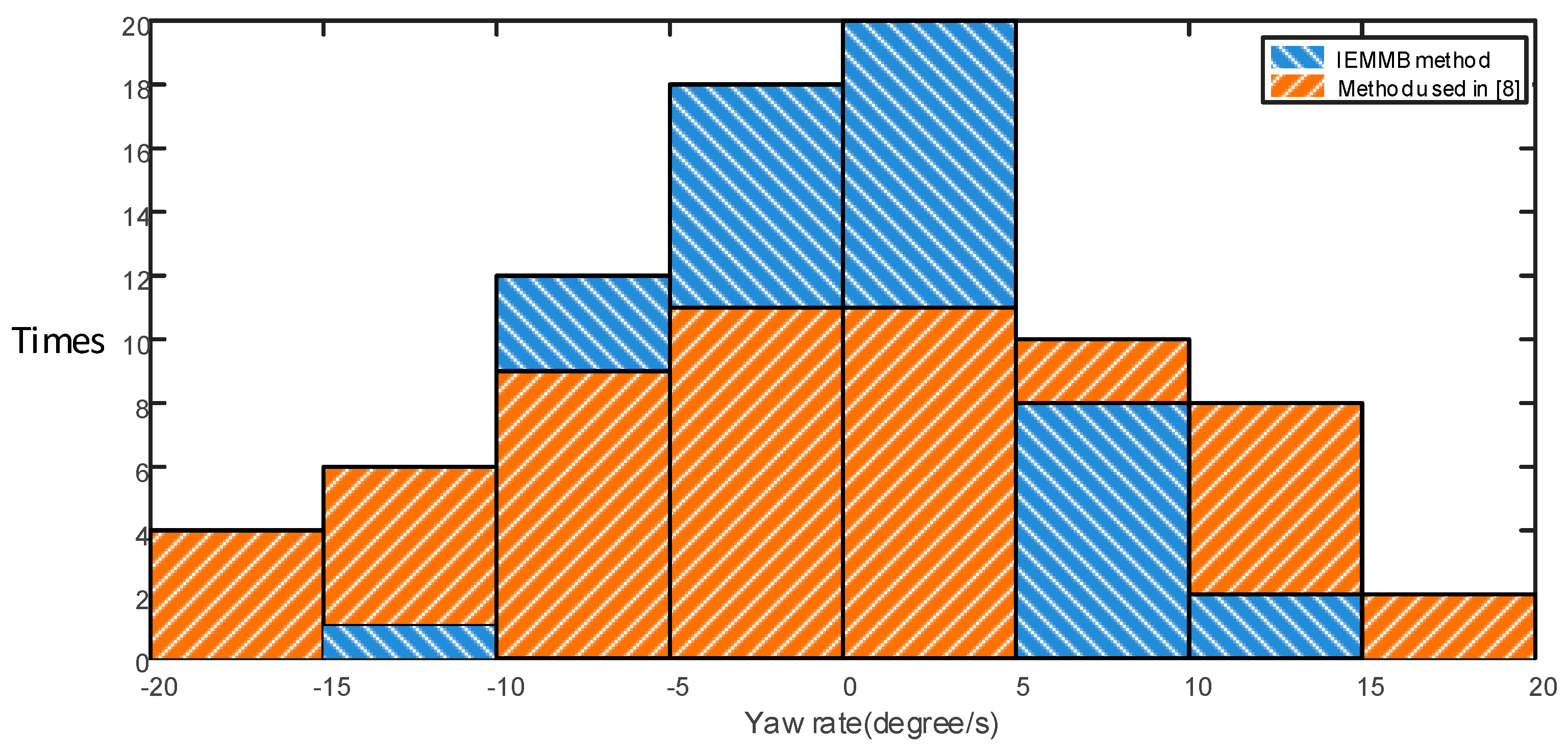
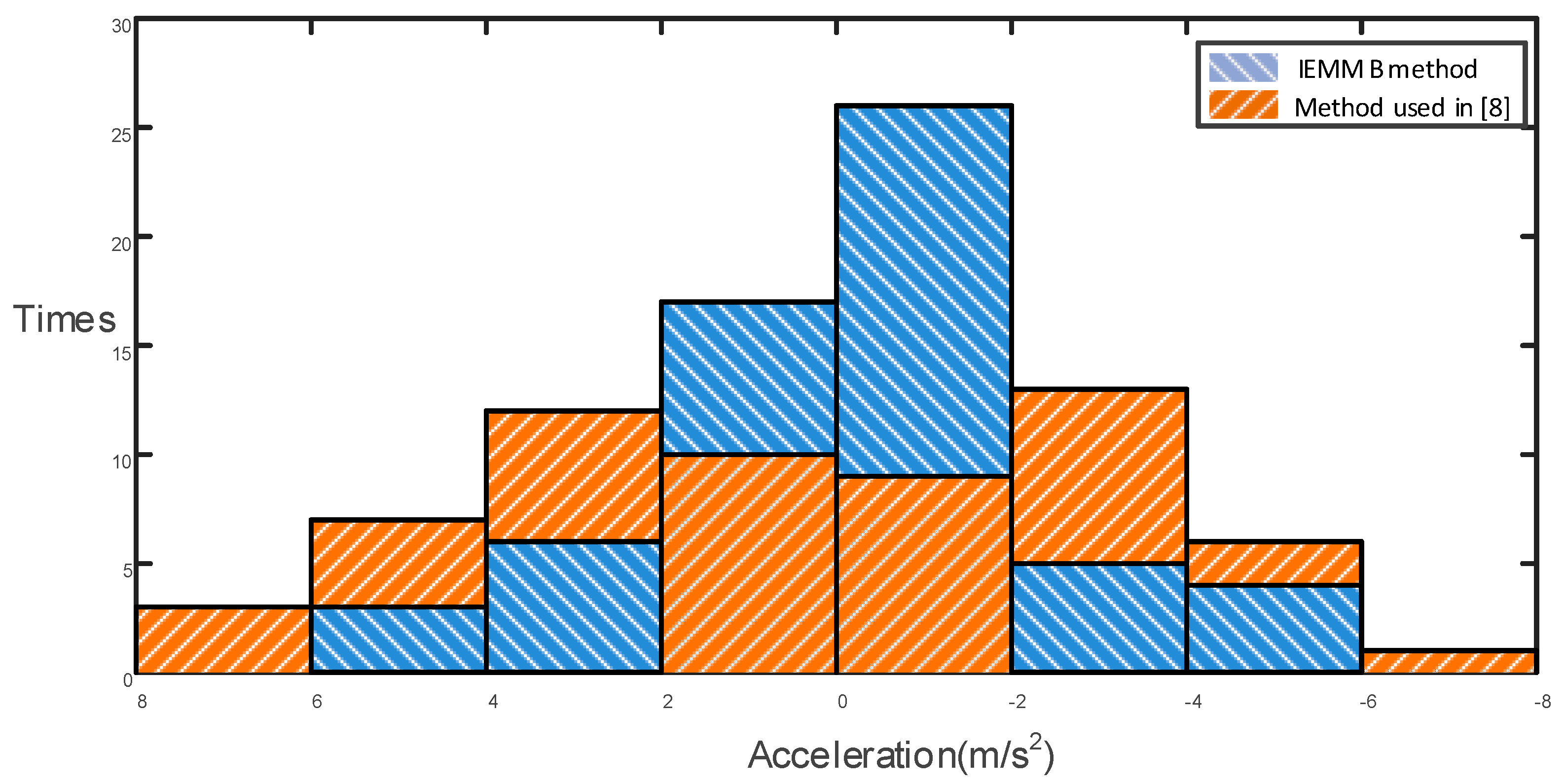
3.2. Performance of Collision Avoidance Method
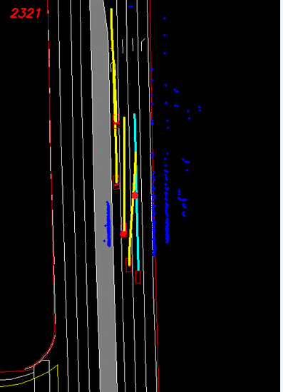
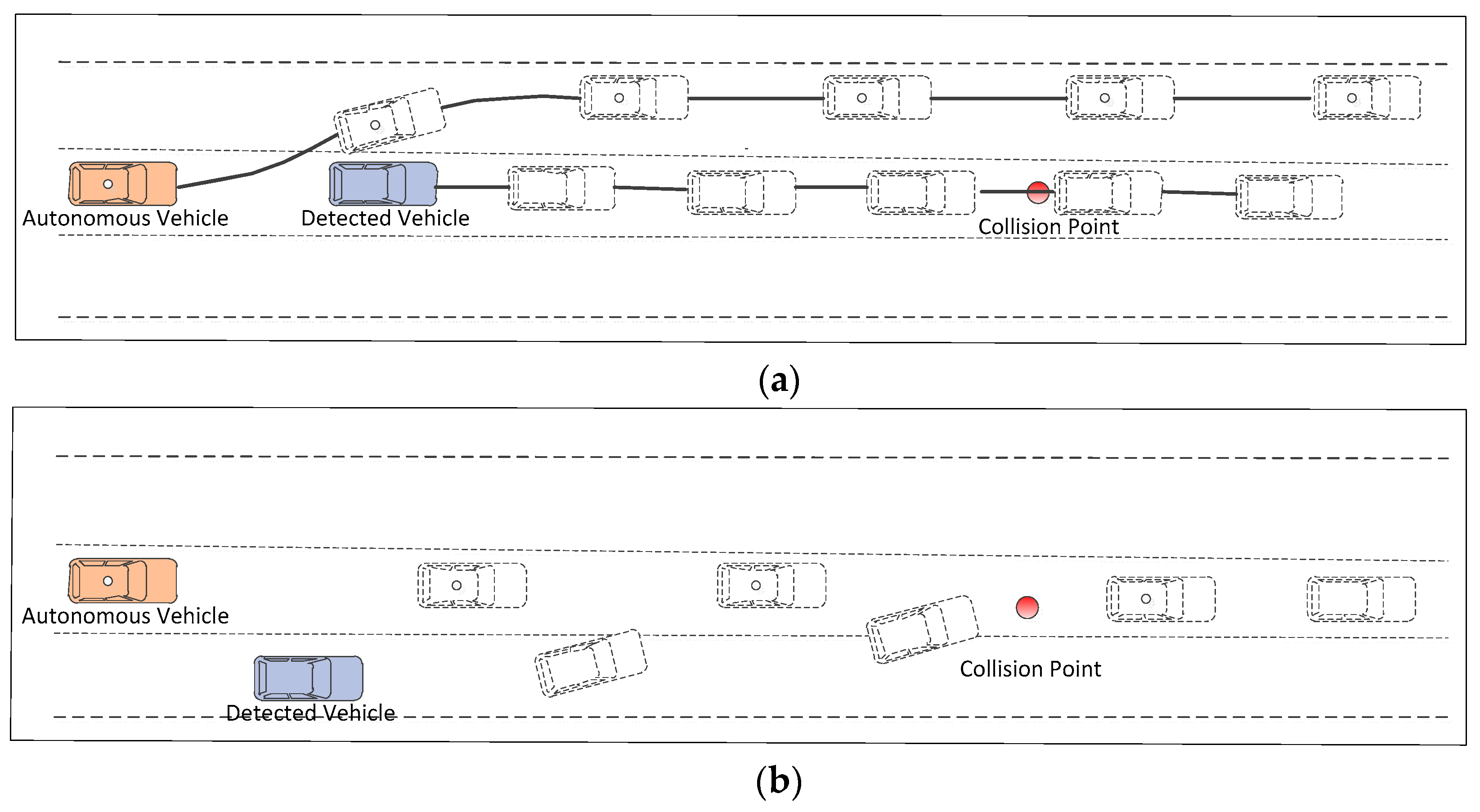
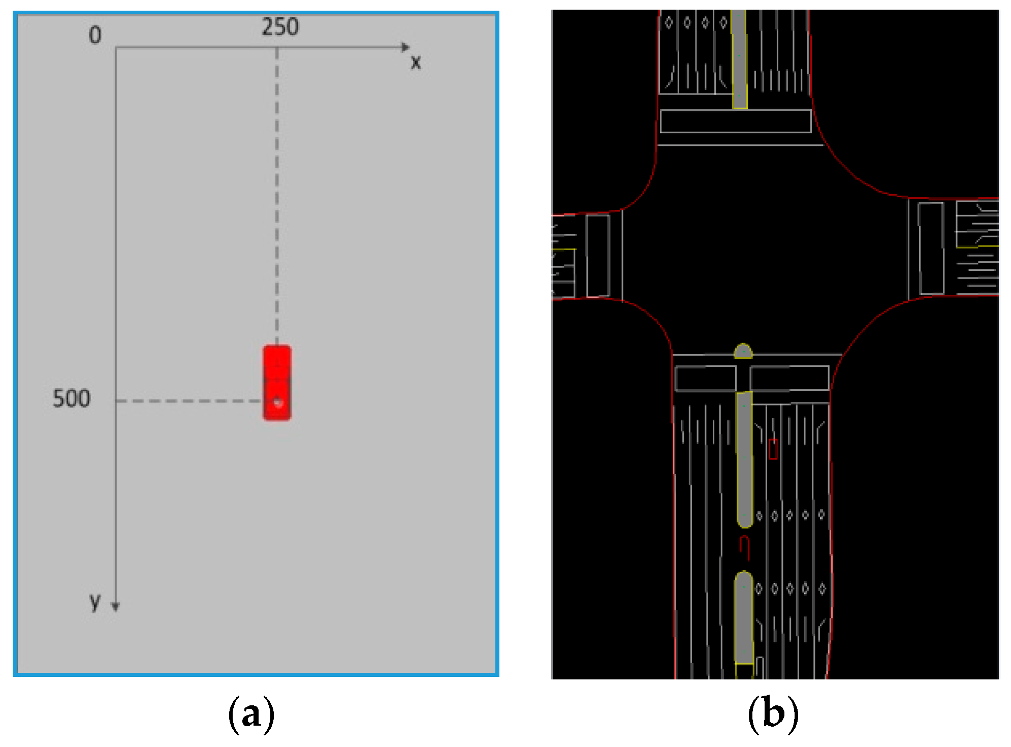
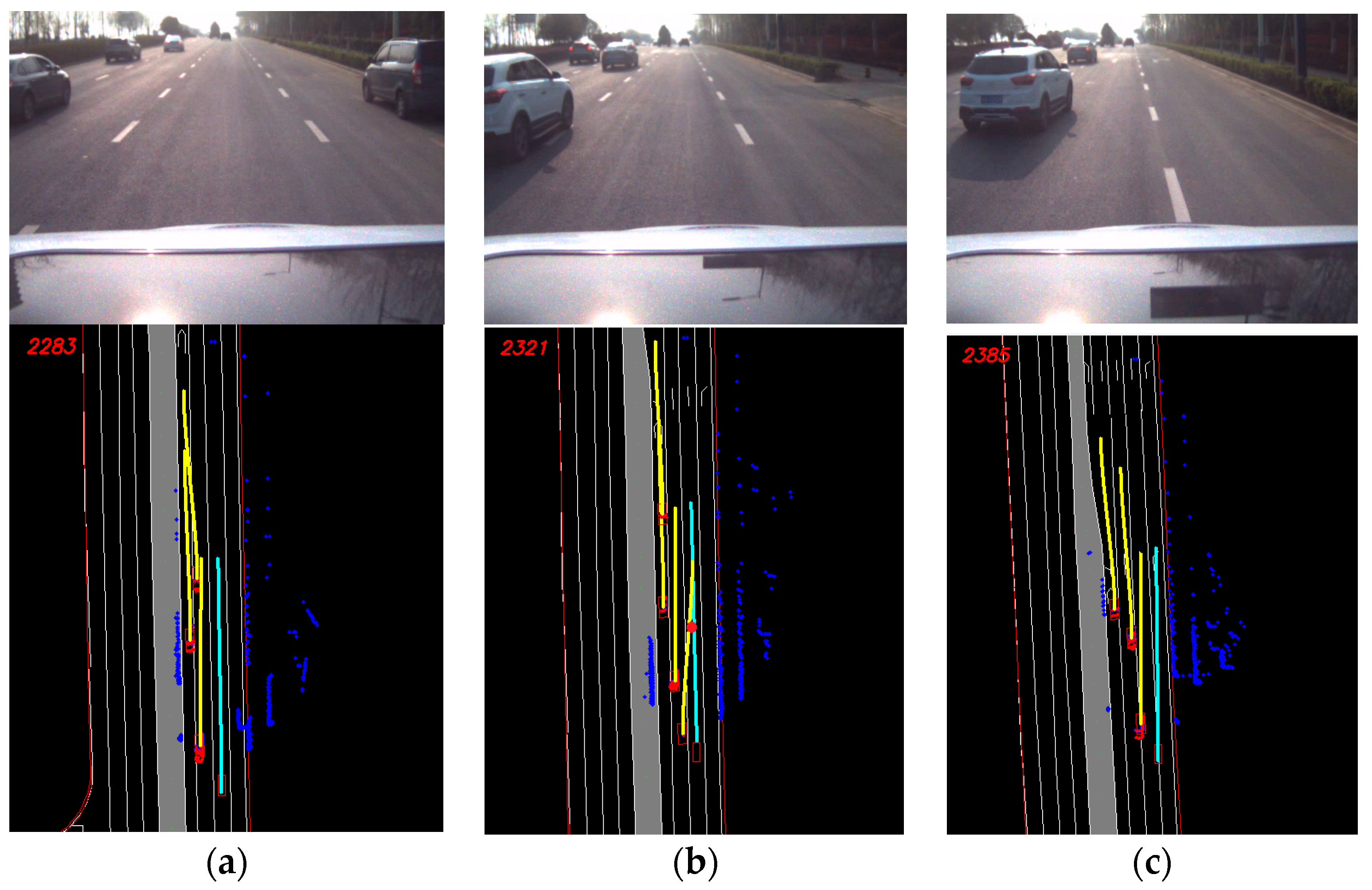
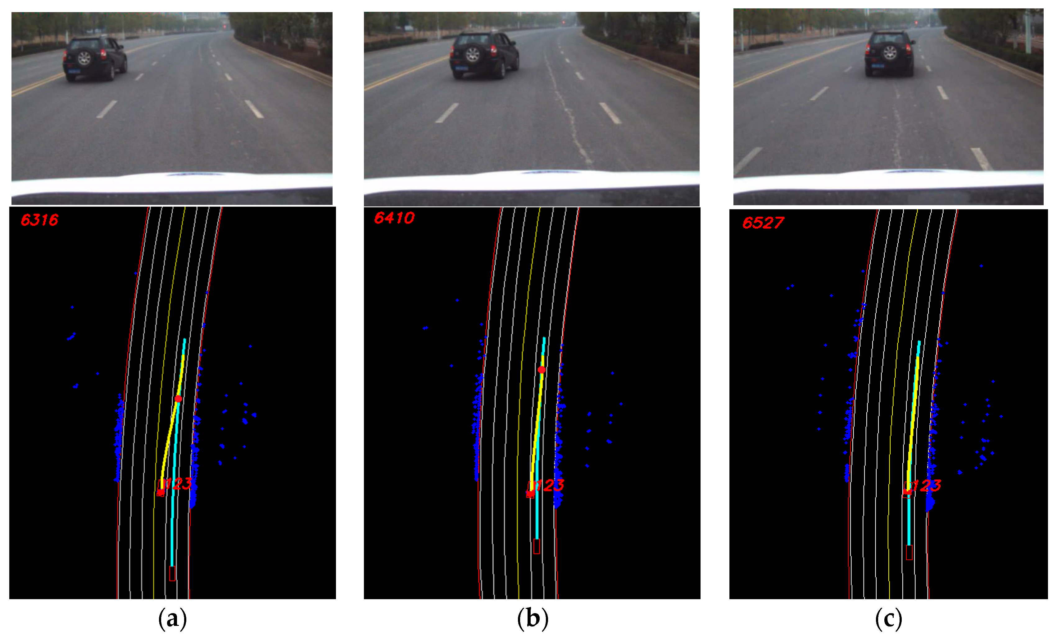
3.3. Typical Collision Avoidance Scenes
4. Conclusions
Acknowledgments
Author Contributions
Conflicts of Interest
Appendix A
Appendix B
| Our Method | Predicted Results | Normal moving | Left lane change | Right lane change | |
| Ground Truth | |||||
| Normal Moving | 270 | 4 | 4 | ||
| Left lane change | 4 | 34 | 0 | ||
| Right lane change | 4 | 0 | 30 | ||
| Method in [11] | Predicted Results | Normal moving | Left lane change | Right lane change | |
| Ground Truth | |||||
| Normal Moving | 249 | 16 | 13 | ||
| Left lane change | 10 | 28 | 0 | ||
| Right lane change | 9 | 0 | 25 | ||
| Our Method | Predicted Results | Normal moving | Left lane change | Right lane change | |
| Ground Truth | |||||
| Normal Moving | 221 | 7 | 5 | ||
| Left lane change | 5 | 33 | 0 | ||
| Right lane change | 4 | 0 | 25 | ||
| Method in [11] | Predicted Results | Normal moving | Left lane change | Right lane change | |
| Ground Truth | |||||
| Normal Moving | 176 | 33 | 24 | ||
| Left lane change | 21 | 17 | 0 | ||
| Right lane change | 15 | 0 | 14 | ||
References
- Pawan, D. Road Safety and Accident Prevention in India: A review. IJAET 2014, 5, 64–68. [Google Scholar]
- IEEE SPECTRUM. Available online: http://spectrum.ieee.org/transportation/advanced-cars/autonomous-vehicles-complete-darpa-urban-challenge (accessed on 1 November 2007).
- The New York Times. Available online: https://www.nytimes.com/interactive/2016/07/01/business/inside-tesla-accident.html?_r=0,July (accessed on 12 July 2016).
- State of California Department of Motor Vehicles. Available online: https://www.dmv.ca.gov/portal/wcm/connect/3946fbb8-e04e-4d52-8f80-b33948df34b2/Google_021416.pdf?MOD=AJPERES (accessed on 23 February 2016).
- Urmson, C.; Anhalt, J.; Bagnell, D.; Baker, C.; Bittner, R.; Clark, M.N.; Dolan, J.; Duggins, D.; Galatali, T.; et al. Autonomous Driving in Urban Environments: Boss and the Urban Challenge. J. Field Robot. 2008, 25, 425–466. [Google Scholar] [CrossRef]
- Ferguson, D. Prediction, Tracking and Avoidance of Dynamic Obstacle in Urban Environments. In Proceedings of the IEEE Intelligent Vehicles Symposium, Eindhoven, The Netherlands, 4–6 June 2008. [Google Scholar]
- Montemerlo, M. Junior: The Stanford Entry in the Urban Challenge. J. Field Robot. 2008, 25, 569–597. [Google Scholar] [CrossRef]
- Xin, Y.; Liang, H.; Mei, T.; Huang, R.; Chen, J.; Zhao, P.; Sun, C.; Wu, Y. A New Dynamic obstacle Collision Avoidance System for Autonomous Vehicles. Int. J. Robot. Autom. 2015, 30, 113–131. [Google Scholar] [CrossRef]
- Stéphanie, L. Context-based Estimation of Driver Intent at Road Intersections. In Proceedings of the IEEE Symposium on Computational Intelligence in Vehicles and Transportation Systems, Singapore, 16–19 April 2013. [Google Scholar]
- Liebner, M. Velocity-Based Driver Intent Inference at Urban Intersections in the Presence of Preceding Vehicles. Intell. Trans. Syst. Mag. 2013, 5, 10–21. [Google Scholar] [CrossRef]
- Gadepally, V.N. Estimation of Driver Behavior for Autonomous Vehicle Applications. Ph.D. Theses, The Ohio State University, Columbus, OH, USA, 2013. [Google Scholar]
- Huang, R.; Liang, H.; Chen, J.; Zhao, P.; Du, M. An intent inference based dynamic obstacle avoidance method for intelligent vehicle in structured environment. In Proceedings of the IEEE International Conference on Robotics and Biomimetics, Zhuhai, China, 6–9 December 2015. [Google Scholar]
- Houenou, A.; Bonnifait, P.; Cherfaoui, V.; Yao, W. Vehicle trajectory prediction based on motion model and maneuver recognition. In Proceedings of the IEEE Intelligent Vehicles Symposium, Gold Coast, Australia, 23–26 June 2013. [Google Scholar]
- Yu, D.; Deng, L. Gaussian Mixture Models. In Automatic Speech Recognition; Springer: London, UK, 2015; pp. 13–21. [Google Scholar]
- Shu, K.N.; Krishnan, T.; Mclachlan, G.J. The EM Algorithm. In Handbook of Computational Statistics; Springer: Berlin/Heidelberg, Germany, 2012; pp. 139–172. [Google Scholar]
- Werling, M.; Ziegler, J.; Kammel, S.; Thrun, S. Optimal trajectory generation for dynamic street scenarios in a Frenét Frame. In Proceedings of the IEEE International Conference on Robotics and Automation, Anchorage, AK, USA, 3–8 May 2010. [Google Scholar]
- Takahashi, A.; Hongo, T.; Ninomiya, Y.; Sugimoto, G. Local Path Planning and Motion Control for AGV in Positioning. In Proceedings of the IEEE/RSJ International Workshop on Intelligent Robots and Systems, Tsukuba, Japan, 4–6 September 1989; pp. 392–397. [Google Scholar]
- Schubert, R.; Richter, E.; Wanielik, G. Comparison and evaluation of advanced motion models for vehicle tracking. In Proceedings of the International Conference on Information Fusion, Cologne, Germany, 30 June–3 July 2008. [Google Scholar]
- Liu, J.; Liang, H.; Wang, Z.; Chen, X. A Framework for Applying Point Clouds Grabbed by Multi-Beam LIDAR in Perceiving the Driving Environment. Sensors 2015, 15, 21931–21956. [Google Scholar] [CrossRef] [PubMed]
- Du, M.; Mei, T.; Liang, H.; Chen, J.; Huang, R.; Zhao, P. Drivers’ Visual Behavior-Guided RRT Motion Planner for Autonomous On-Road Driving. Sensors 2016, 16, 102. [Google Scholar] [CrossRef] [PubMed]
- Chen, J.; Zhao, P.; Liang, H.; Mei, T. Motion Planning for Autonomous Vehicle Based on Radial Basis Function Neural Network in Unstructured Environment. Sensors 2014, 14, 17548–17566. [Google Scholar] [CrossRef] [PubMed]
- Karjanto, J.; Yusof, N.M. Comfort Determination in Autonomous Driving Style. In Proceedings of the AutoUI, Nottingham, UK, 1–3 September 2015. [Google Scholar]


| Examples | |||
|---|---|---|---|
| 0.9 | −0.1 | 1.91 | |
| 0.40 | 1.76 | 0.69 | |
| Vector_1 (left lane change) | 1.1 | −0.8 | 1.6 |
| Vector_2 (normal moving) | 0.6 | 0.4 | 0.8 |
| Z-score of Vector_1 | 0.5 | −0.82 | 0.45 |
| Z-score of Vector_2 | −0.75 | 0.28 | −1.61 |
| Maneuver Type | Normal Moving | Left Lane Change | Right Lane Change | |
|---|---|---|---|---|
| Road Type | ||||
| Straight Road | 50 | 50 | 50 | |
| Winding Road | 50 | 50 | 50 | |
| Methods | Intent Types | True Positive | False Positive | False Negative | Precision Rate | Recall Rate | F-Score |
|---|---|---|---|---|---|---|---|
| Proposed Method | Normal moving | 270 | 8 | 8 | 97.1% | 97.1% | 97.1% |
| Left lane changes | 34 | 5 | 4 | 87.2% | 89.5% | 88.6% | |
| Right lane change | 30 | 3 | 4 | 90.9% | 88.2% | 89.5% | |
| Method in [11] | Normal moving | 249 | 19 | 29 | 92.9% | 89.6% | 91.2% |
| Left lane change | 28 | 16 | 10 | 63.6% | 73.7% | 68.3% | |
| Right lane change | 25 | 13 | 9 | 65.8% | 73.5% | 69.4% |
| Methods | Intent Types | True Positive | False Positive | False Negative | Precision Rate | Recall Rate | F-Score |
|---|---|---|---|---|---|---|---|
| Proposed Method | Normal moving | 221 | 9 | 12 | 96.1% | 94.8% | 95.4% |
| Left lane changes | 33 | 7 | 5 | 82.5% | 86.8% | 84.6% | |
| Right lane change | 25 | 5 | 4 | 83.3% | 86.2% | 84.7% | |
| Method in [11] | Normal moving | 176 | 36 | 57 | 83.0% | 75.5% | 79.1% |
| Left lane change | 17 | 33 | 21 | 34% | 44.7% | 38.6% | |
| Right lane change | 14 | 24 | 15 | 36.8% | 48.3% | 41.8% |
© 2017 by the authors. Licensee MDPI, Basel, Switzerland. This article is an open access article distributed under the terms and conditions of the Creative Commons Attribution (CC BY) license (http://creativecommons.org/licenses/by/4.0/).
Share and Cite
Huang, R.; Liang, H.; Zhao, P.; Yu, B.; Geng, X. Intent-Estimation- and Motion-Model-Based Collision Avoidance Method for Autonomous Vehicles in Urban Environments. Appl. Sci. 2017, 7, 457. https://doi.org/10.3390/app7050457
Huang R, Liang H, Zhao P, Yu B, Geng X. Intent-Estimation- and Motion-Model-Based Collision Avoidance Method for Autonomous Vehicles in Urban Environments. Applied Sciences. 2017; 7(5):457. https://doi.org/10.3390/app7050457
Chicago/Turabian StyleHuang, Rulin, Huawei Liang, Pan Zhao, Biao Yu, and Xinli Geng. 2017. "Intent-Estimation- and Motion-Model-Based Collision Avoidance Method for Autonomous Vehicles in Urban Environments" Applied Sciences 7, no. 5: 457. https://doi.org/10.3390/app7050457
APA StyleHuang, R., Liang, H., Zhao, P., Yu, B., & Geng, X. (2017). Intent-Estimation- and Motion-Model-Based Collision Avoidance Method for Autonomous Vehicles in Urban Environments. Applied Sciences, 7(5), 457. https://doi.org/10.3390/app7050457