Compensation for Group Velocity of Polychromatic Wave Measurement in Dispersive Medium


Abstract
:1. Introduction
2. Group Velocity Measurement Based on Electromagnetic Wave Theory
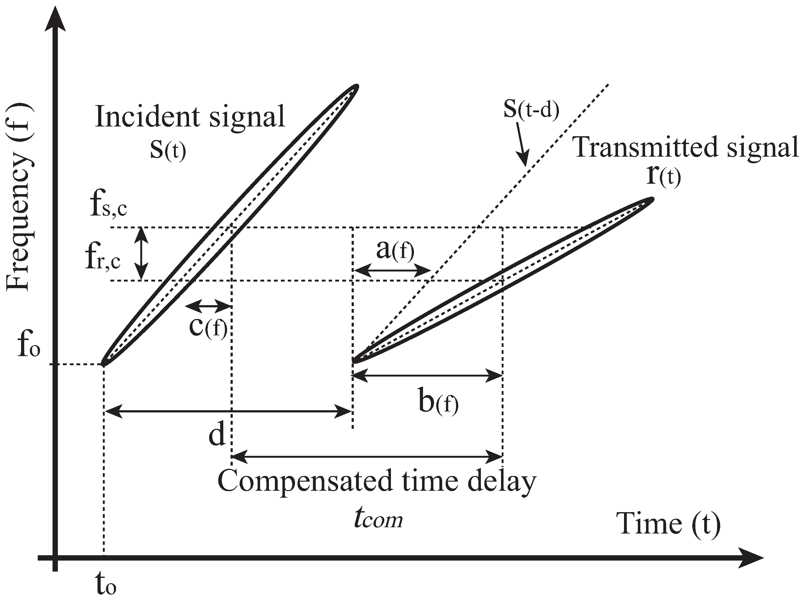
3. Compensation of Group Velocity in Dispersive Medium
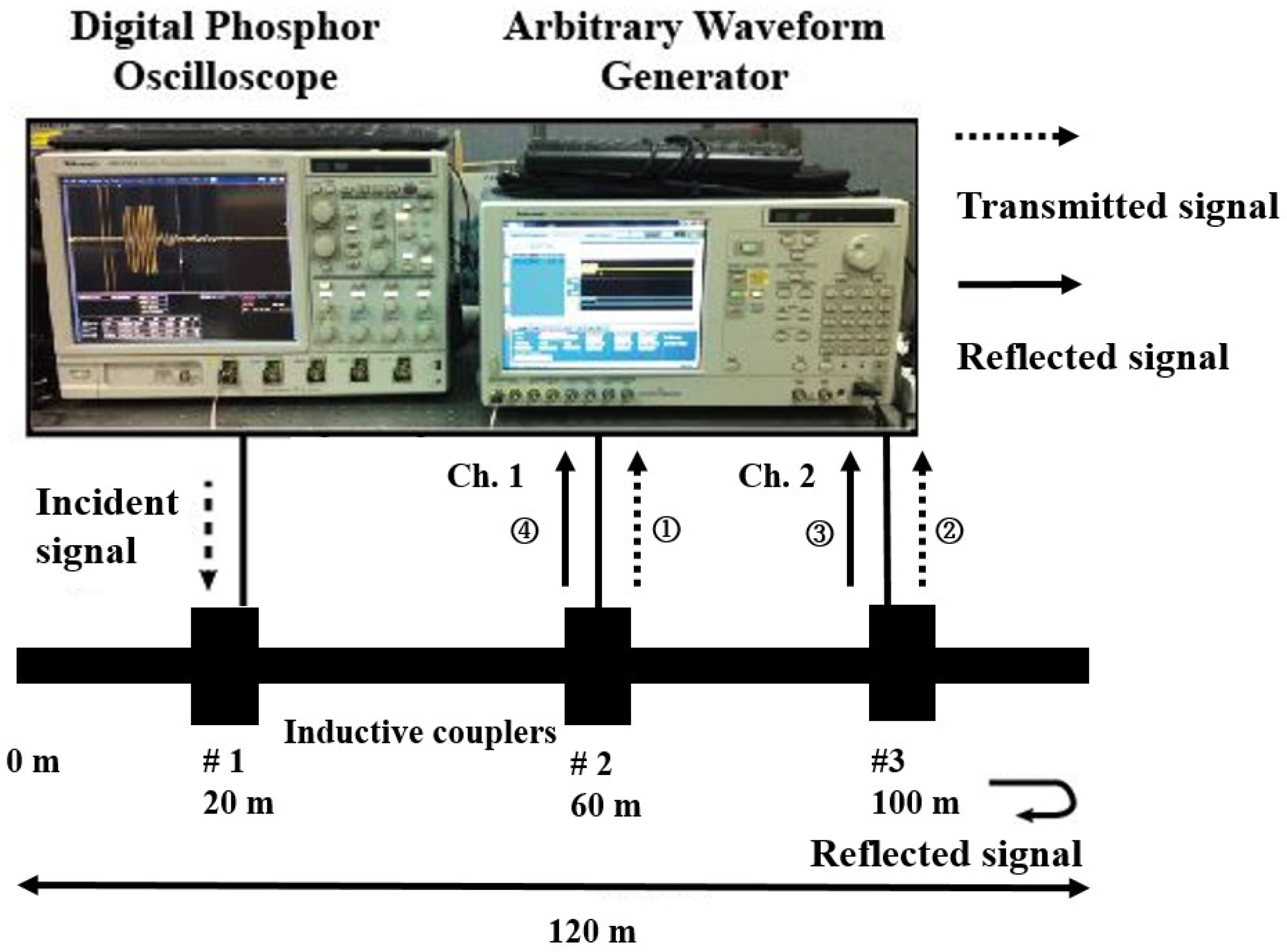
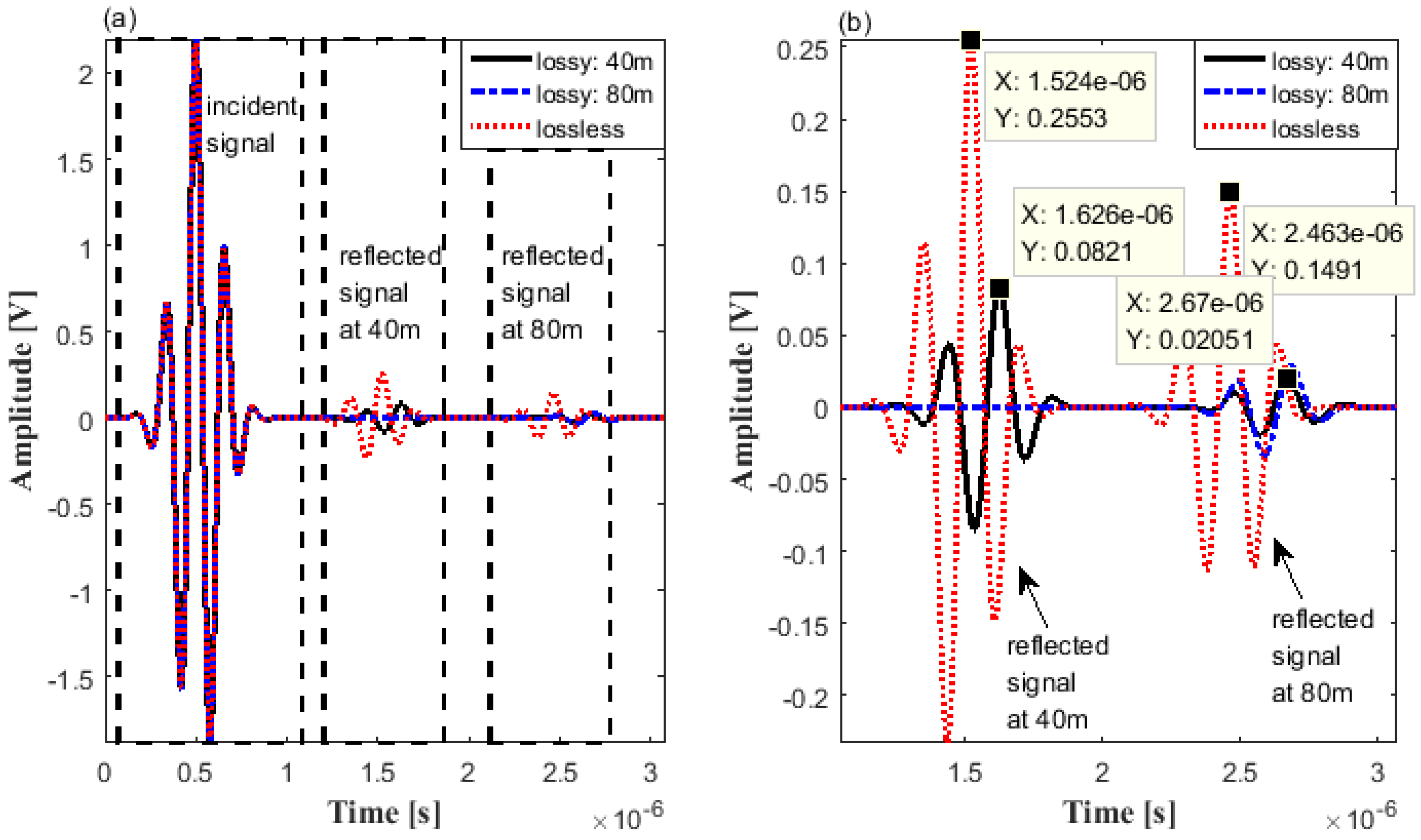
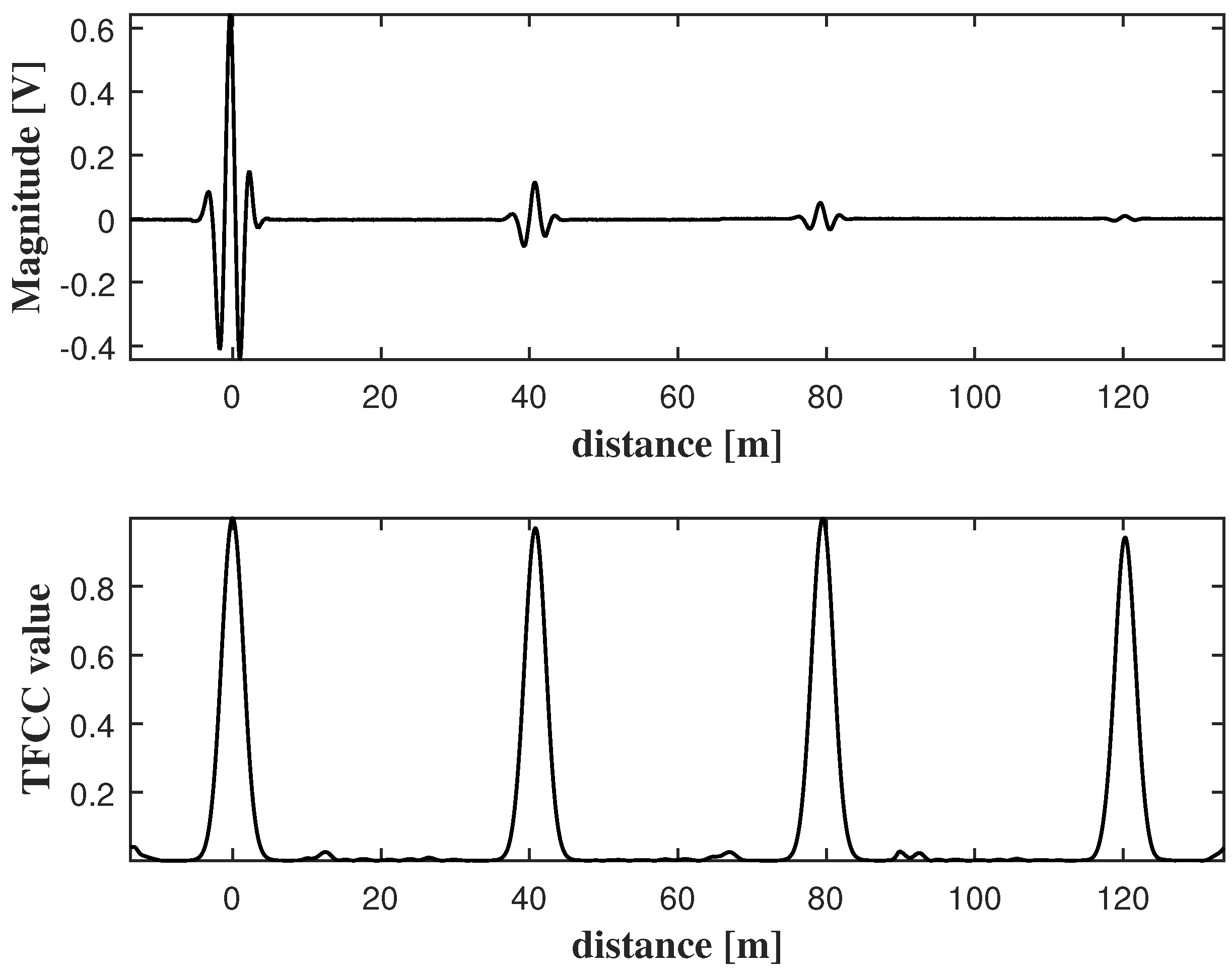
4. Experimental Results
5. Conclusions
Author Contributions
Conflicts of Interest
References
- Cho, J.; Kim, H.; Jung, K.-Y. Simple transmission line model suitable for the electromagnetic pulse coupling analysis of twisted-wire pairs above ground. IEICE Electron. Express 2016, 13, 20160149. [Google Scholar] [CrossRef]
- Chowdary, K.M.; Majetich, S.A. Frequency-dependent magnetic permeability of Fe10Co90 nanocomposites. J. Phys. D Appl. Phys. 2014, 47, 175001. [Google Scholar] [CrossRef]
- Chang, S.J.; Lee, C.K.; Lee, C.-K.; Han, Y.J.; Jung, M.K.; Park, J.B.; Shin, Y.-J. Condition monitoring of instrumentation cable splices using Kalman filtering. IEEE Trans. Instrum. Meas. 2015, 64, 3490–3499. [Google Scholar] [CrossRef]
- Lee, C.K.; Park, J.B.; Shin, Y.J.; Yoon, T.S. High resolution LFMCW radar system using model-based beat frequency estimation in cable fault localization. IEICE Electron. Express 2014, 11, 20130768. [Google Scholar] [CrossRef]
- Lee, S.H.; Lee, C.K.; Park, J.B.; Choi, T.H. Diagnostic method for insulated power cables based on wavelet energy. IEICE Electron. Express 2013, 10, 20130335. [Google Scholar] [CrossRef]
- Kwak, K.S.; Doo, S.; Lee, C.K.; Yoon, T.S. Reduction of the blind spot in the time-frequency domain reflectometry. IEICE Trans. Electron. 2008, 5, 265–270. [Google Scholar] [CrossRef]
- Lee, C.K.; Kwak, K.S.; Yoon, T.S.; Park, J.B. Cable Fault Localization Using Instantaneous Frequency Estimation in Gaussian-Enveloped Linear Chirp Reflectometry. IEEE Trans. Instrum. Meas. 2013, 62, 129–139. [Google Scholar] [CrossRef]
- Shin, Y.J.; Song, E.S.; Kim, J.W.; Park, J.B.; Yook, J.G.; Powers, E.J. Time-frequency domain reflectometry for smart wiring systems. Proc. SPIE 2002, 4791. [Google Scholar] [CrossRef]
- Chang, S.J.; Lee, C.K.; Shin, Y.-J.; Park, J.B. Multiple Resolution Chirp Reflectometry for Fault Localization and Diagnosis High Voltage Cable in Automotive Electronics. Meas. Sci. Technol. 2016, 27, 125006. [Google Scholar] [CrossRef]
- Selesnick, I.W.; Figueiredo, M.A.T. Signal restoration with overcomplete wavelet transforms: comparison of analysis and systhesis priors. Proc. SPIE 2009, 7446. [Google Scholar] [CrossRef]


| Group Velocity | |||
|---|---|---|---|
| Cable Length: 40 m | Cable Length: 80 m | Cable Length: 120 m | |
| TFCC accuracy | |||
| proposed method accuracy | |||
| measurement value | |||
© 2017 by the authors. Licensee MDPI, Basel, Switzerland. This article is an open access article distributed under the terms and conditions of the Creative Commons Attribution (CC BY) license (http://creativecommons.org/licenses/by/4.0/).
Share and Cite
Chang, S.J.; Moon, S.-I. Compensation for Group Velocity of Polychromatic Wave Measurement in Dispersive Medium. Appl. Sci. 2017, 7, 1306. https://doi.org/10.3390/app7121306
Chang SJ, Moon S-I. Compensation for Group Velocity of Polychromatic Wave Measurement in Dispersive Medium. Applied Sciences. 2017; 7(12):1306. https://doi.org/10.3390/app7121306
Chicago/Turabian StyleChang, Seung Jin, and Seung-Il Moon. 2017. "Compensation for Group Velocity of Polychromatic Wave Measurement in Dispersive Medium" Applied Sciences 7, no. 12: 1306. https://doi.org/10.3390/app7121306
APA StyleChang, S. J., & Moon, S.-I. (2017). Compensation for Group Velocity of Polychromatic Wave Measurement in Dispersive Medium. Applied Sciences, 7(12), 1306. https://doi.org/10.3390/app7121306