1. Introduction
In an increasingly connected world, network security is a pressing issue facing many organizations. Modern networks consist of a myriad of devices sharing data through a variety of services and each with a private data store that they wish to keep safe [
1,
2]. On top of this, many devices are connected to other networks or the Internet, exposing them to threats from outside attackers, including compromising network availability, damaging devices, and stealing data.
Given the complexity of the network and the range of possible damages, many network administrators have turned to game theory to model network vulnerabilities and determine an optimal defense strategy [
3]. Game models allow us to predict, to a degree, the results of defensive actions, which offers an enormous advantage over simple heuristics. Modification of the model allows for quick response to new attacker strategies. Filtering network security decisions through a game-based model helps to allocate limited resources, calculate risks, and automate network defense [
4].
Xiao et al. [
5] surveyed ongoing usage of game theory in cyber security and have identified a variety of applications, each adapted to different security scenarios. Consistent in their approach is the idea of modeling the network defense as a two-player game between an attacker and a defender. Kordy proved that attack-trees can be extended to include defender actions [
6], to create attack-defense trees, which are essentially a representation of actions in a two-player zero-sum game [
7].
Given the advantages of game modeling, the security industry would benefit from research in determining an optimal defense strategy in network security games. This article attempts to find an optimal defense strategy for a two-player zero-sum game. We use an information-incomplete model with simultaneous game play and multiple objectives. This model is a more realistic representation of actual network security, as the defender needs to balance different goals, during an attack. Specifically, we attempt to automate attacker and defender behavior and determine a rapid method to find an optimal defense strategy.
Current application of game theory models tends to focus on finding the Nash equilibrium for single-objective symmetric games. Our proposal offers a major improvement by using multiple objective reinforcement learning to ensure continuous improvement. This approach, while not unique, is scarcely researched and has not been applied to network security games. Examples outside of network security include Kamis and Gomaa implementing a multi-objective learning algorithm for traffic signal control [
8] and van Moffaert [
9] describing methods for scalarized reinforcement. We believe that there is a clear need for this approach in network security games.
We further improve the basic Q-learning approach by combining it with a multi-objective specific optimization algorithm, namely Pareto optimization. This method has been used in network games by Eisenstadt [
10] to show that Pareto optimization can be used to remove non-optimal strategies. The advantages of the Pareto approach are not undisputed, as Ikeda et al. [
11] doubts the effectiveness of using Pareto domination to find optimal solutions. This article shows that using Pareto optimization actually improves the reinforcement learning approach to find an optimal defense strategy for a network security game.
There is a plethora of research addressing the issues in the context of networking using game-theoretic models, bandwidth allocation [
12,
13,
14,
15], flow control [
16,
17,
18] price modeling [
19,
20] and routing [
21,
22]. Methodological analysis of decision-making in the context of security has paved the way for using game theory to model the interactions of agents in security problems [
23,
24]. Game theory provides mathematical tools for the decision-maker to choose optimal strategies from an enormous search space of what-if scenarios [
25]. There has been a growing body of research towards game-theoretic approach on network security problems [
24].
Roy et al. [
26] and Manshaei et al. [
4] have conducted comprehensive surveys of the field showing that game theory serves as an excellent tool for modeling security in computer networks, since securing a computer network involves an administrator trying to defend the network while an attacker tries to harm the network.
Roy categorized game-theoretic network security models into six groups [
26]. They are (1) the perfect information game—all the players are aware of the events that have already taken place; (2) the complete information game—all the players know the strategies and payoffs of the other players; (3) the Bayesian game—where strategies and payoffs of others are unknown and Bayesian probability is used to predict them; (4) the static game—a one-shot game where all of the players play at once; (5) the dynamic game—a game with more than one stage in which players consider the subsequent stages; and (6) the stochastic game—games involving a probabilistic transition of stages.
Sallhammar [
27] has proposed a stochastic approach to study vulnerabilities and system’s security and dependability in certain environments. The model provides real-time assessment. Unlike our model the proposed model is more inclined toward security risk assessment, dependability, and trustworthiness of the system. In addition to that, their model assumes vulnerabilities are unknown, whereas in our work the possible attack and defense scenarios are known to both agents.
Liu et al. [
28] analyzed interaction between attacking and defending nodes in ad-hoc wireless networks using a Bayesian game to approach. The proposed hybrid Bayesian-approach Intrusion Detection System (IDS) saves significant energy while reducing the damage inflicted by the attacker. In this model, the stage games are considered Bayesian static since the defender’s belief update requires constant observation of the attacker’s action at each stage. Karim et al. [
29] have proposed a similar model that uses collaborative method for IDS. The dynamic nature of this multi-stage game is similar to our model. In contrast to their model, we analyze the best defense strategy for a defender in heterogeneous network.
In this paper, we study the behavior of an agent (defender) who tries to maximize three goals: the cost difference, the number of uncompromised data nodes, and network availability. The agents iteratively play the game and stage transition uses a probability function. Thus, in this article, we focus on stochastic game with multiple objectives. In multi-objective mathematical programming there is no single optimal solutions [
30]. Since all objective functions are simultaneously optimized, the decision maker searches for the most preferable solution, instead of the most optimal solution [
31].
1.1. Pareto Optimization
The administrator has a limited amount of resources and achieving complete security is unattainable [
32,
33]. Thus, a realistic approach is to find an optimal strategy that maximizes the performance of the network with a minimum cost despite known vulnerabilities [
34,
35,
36,
37,
38,
39,
40,
41,
42,
43,
44,
45,
46]. Similarly, the attacker has a limited amount of resources. The knowledge of possible actions for both players allows participants to discover the potential actions and their best counter action [
37]. Thus, both participants are forced to maximize their utility from multiple goal perspectives [
38]. Pareto optimality is a state of resource allocation that addresses the issue of cost/benefit trade off. In a Pareto optimal state, no goal can be further improved without making the other goals worse off.
Gueye et al. [
32] have proposed a model for evaluating vulnerabilities by quantifying corresponding Pareto optima using the supply-demand flow model. The derived vulnerability to the attack metric reflects the cost of a failed link, as well as the attacker’s willingness to attack a link.
The Pareto front separates the feasible region from an infeasible region [
39]. The optimal operating point is computed by considering a network utility function. In this model, vulnerability to the attack metric is dependent on network topology, which makes it unsuitable for fully connected networks [
40].
Guzmán and Bula proposed a bio-inspired metaheuristic hybrid model that addresses the bi-objective network design problem. It combines Improved Strength Pareto Evolutionary Algorithm—SPEA2 and the Bacterial Chemotaxis Multi-objective Optimization Algorithm (BCMOA) [
41]. The Pareto-optimal points approximations are faster than SPEA2 and Binary-BCMOA, however this method is not applicable to our model since we include more than two objectives.
In recent years, multi-objective reinforcement learning has emerged as a growing area of research. Fang et al. [
42] used reinforcement learning to enhance the security scheme of cognitive radio networks by helping secondary users to learn and detect malicious attacks and nodes. The nodes then adapt and dynamically reconfigure operating parameters.
1.2. Reinforcement Learning
Reinforcement learning (RL) is a machine learning technique used by software agents to determine a reward maximizing strategy for given environment [
43]. Attack-defense games that use RL provide users with the capability to analyze hundreds of possible attack scenarios and methods for finding optimal defense strategies with predicted outcomes [
26]. The technique is derived from behavioral psychology, where agents are encouraged to repeat past beneficial behavior and discouraged from repeating harmful behavior [
44,
45]. This article uses a Q-learning implementation of reinforcement learning. As such, it is best to describe the technique using the specific Q-learning.
Lye et al. [
37] proposed a two-player stochastic, general-sum game with a limited set of attack scenarios. The game model consists a seven-tuple set of network states, actions, a state transition function, a reward function, and a discount factor, resulting in, roughly, 16 million possible states. However their work only considered 18 network states. The game topology consists of only four nodes with four links. This model is inefficient if a large number of nodes is introduced to the network. One of the key disadvantages of the model is that it uses full state spaces, making it inefficient. The model has some resemblances to ours as we employ reinforcement learning as the state transition probability calculation method. In this paper, we address a similar situation with much larger set of network nodes.
RL has the problem of a combinatorial explosive state space [
46]. In order to learn Q-values, each agent (attacker or defender) is required to store Q-values in a table. Each entry in the Q-table represents a state reward for each action by one agent (attacker) to a corresponding action for that of other agent (defender). Thus, the action space is an exponential of the number of agents. In RL, the agent learns by trial-and-error, by repeatedly going through the stages. The iterative process of taking an action and obtaining a reward allows the agent to gain percepts of the dynamic environment.
Several methods have been proposed to reduce the size of the state space and most methods involve scalarizing the reward function and learning with the resulting single-objective function [
47]. Girgin et al. [
48] have proposed a method to address the issue by constructing a tree to locate common action sequences of possible state for possible optimal policies. The subtasks that have almost identical solutions are considered similar. The repeated smaller subtasks that have a hierarchical relationship among them are combined into a common action sequence. The intuition behind this method is that, in most realistic and complex domains, the task that an agent tries to solve is composed of various subtasks and has a hierarchical structure formed by the relations between them [
49,
50], and the tree structure with common action sequence prevents agents going through inefficient repetition.
Tuyls et al. [
51] used a decision tree to overcome the problem. The tree is created online allowing agent to shift attention to other areas of the state space. Nowe and Verbeek’s approach to limit the state space is to force the agents to only model agents relevant to themselves. Inspired by biological systems, Defaweux et al. [
52] have a proposed a similar system to address the product space problem, in which they only take a
niche combination of agents who have relevant impact on reward function. Those who have a little impact on reward function are discarded.
Another method to resolve the issue of combinatorial explosion of state space is generalization. The goal is to have a smaller number of states (subset), which is useful to approximate a much larger set of states. This method speeds up learning and reduces the storage space required for lookup tables. However the (accuracy) quality of this method depends on the accuracy of the function approximation that takes example from target function mappings and attempts to generalize to entire function [
53].
In our proposed model, we address the issue of a large state space by using Pareto optimization. The Pareto sets (Pareto fronts) contain all the optimal solutions for a given defense action. Instead of taking all the actions as inputs for the Q-learning function, we take a subset of the actions (Pareto front of the player’s actions), improving speed of learning. The sets of dominated actions are eliminated, leaving only optimal Pareto fronts. The purpose is to let agents learn from the superior set of actions and make the learning process faster.
3. Game Model on Pareto Optima and Q-learning
3.1. Game Definition
The network attacker and defender interaction can be modelled as an information-incomplete two-player zero-sum game. Using such a model, we will teach our software agent to determine the optimal action when confronted with an actual network attack [
37]. The specific network interaction we wish to model is described as the following game:
Here, is the network, is the set of all possible states the game can be in; is the set of possible actions that an attacker can perform on a node; is the set of possible actions that a defender can perform on a node; is the state transition function; is the reward function defined in Equation (3); and is a discount factor. refers to the solution space for the reward function.
A network
consists of a set of nodes connected by edges. Each node represents a hardware device, which runs several services, can be infected by a virus, and contains data. The value/weight of the services is given by
, the value of keeping the node virus free is
, and the value of the data on the node is
. These values can differ per node. An edge represents the connection between two nodes. If two nodes are running the same service, they will use a connecting edge to communicate.
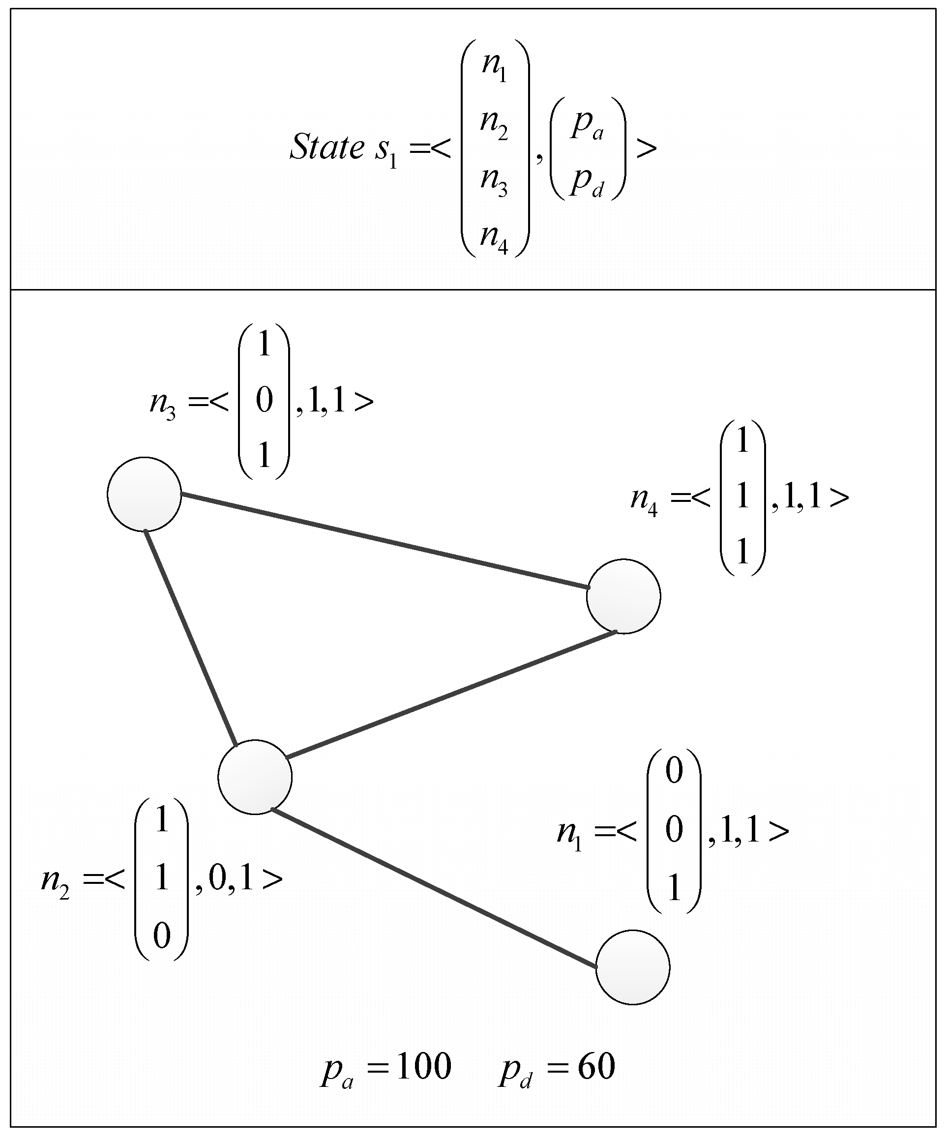
A game state is a combination of the network state and each player’s resource points. The network state is the state of all the nodes, i.e., which services are running on the node, if it is infected by a virus, and whether or not the data has been stolen, and the state of all the edges identified by service availability. Resource points are points that players can spend to perform an action.
The players can only perform actions on the nodes, so the network state is simply the state of the nodes. Let
be the state of the nodes. In the node state,
is a vector showing which services are running on the node (1 = running and 0 = down),
indicates whether or not the node has been virus free (1 = virus-free and 0 = infected) and
indicates whether or not the data is secure (1 = secure and 0 = data is stolen).
In this game, we introduce the concept of resource points. From existing research, we know it is common to assume that each action taken by a player has an associated cost. To keep track of costs, we start a game, by giving each player a fixed set of resource points. The resource points tell us if a player can afford to take a certain action, e.g., if the cost of an action exceeds the available resource points, the player cannot take that action. If a player runs out of resource points, the game ends. Let p be a vector containing the player resource points:
The final definition of a game state is
.
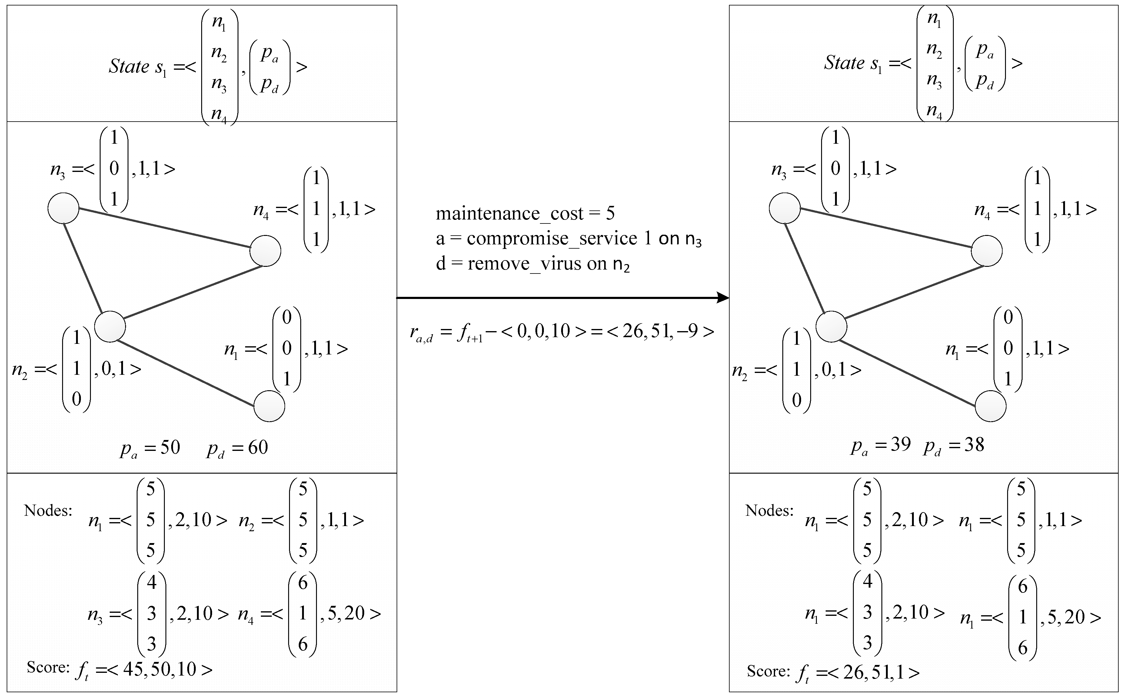
Figure 4 shows a game state with compromised services in
n1,
n2, and
n3 and a virus installed in
n2.
We do not need to formally define the state transition function P. The game will use a combined Pareto-Q-learning algorithm to determine the best policy for the defender and attacker. Hence, Q-values will be determined iteratively according to Equation (8), rather than by the explicitly defined function of Equation (6). Equation (8) does not require an explicitly-defined state transition function.
3.2. Game Rules
This game uses the following actions on a node for the attacker and defender (the cost is shown in brackets):
A = {compromise_service (6), install_virus (12), steal_data (8), nothing (0)}
D = {restore_service (12), remove_virus (12), nothing (0)}
A player can perform any of the above action on a single node. The actual action sets defined in Equations (16) and (17) are a subset of the combination of one of the above actions and the nodes in the network. Assuming that n is the nodes of the network as defined in Equation (13). The subset contains all the valid actions for the current state.
The game is played as follows: At a given time , the game is in state . If all the data is stolen, the game ends. If not, check the player’s resource points. If one of the players has enough resource points to do anything other than nothing, they can perform an action. The game ends as soon as one of the following ending conditions is met:
- -
The attacker brings down all the services (network availability is zero), the game ends.
- -
The attacker manages to steal all the data or infect all the nodes, the game ends
- -
Either the attacker or the defender can no longer make a move, the game ends.
Performing an action: The attacker chooses an action from
and performs it, then the defender chooses an action from
and performs it. The game determines the next state s
t+1 according to the transition function
. The rewards for that state transition are calculated and the goals are updated with the rewards. The game transitions to state
and time
. See
Figure 5 for a state transition
Transitioning to a new state: Transitioning to a new state involves three things: (1) modify the network state according to the performed actions; (2) subtract the cost of the performed action from the corresponding player’s resource points; (3) subtract one resource point for each compromised service and one resource point for each installed virus from the attacker’s resource points; this is a cost for keeping the nodes compromised.
Valid actions: compromise_service—an attacker can compromise any service that is not yet compromised.
install_virus: an attacker can install a virus on any node that is currently virus free.
steal_data: an attacker can steal data from any node that has a virus installed.
restore_service: a defender can restore any service that is compromised.
remove_virus: a defender can remove a virus from any node that has a virus installed.
nothing: either attacker or defender can choose to do nothing.
3.3. Goal Definition
This is a zero-sum game, thus, the goals for the attacker and defender are the inverse of each other, meaning that if the defender aims to maximize a score, the attacker aims to minimize it. The game score at a given time
, where the game is in state
, is defined as:
- -
= score for the network availability;
- -
= score for the node security;
- -
= score for the defense strategy cost effectiveness
The score for network availability is defined as the sum of the value of communicating services.
Keeping the nodes secure means keeping them virus-free and making sure the attacker did not steal the data. Let
be the state of node in the network, defined in Equation (13), such that
An effective defense strategy means that the defender expended as few resource points as possible while defending the network. The score for the defense strategy cost effectiveness is the difference in resource points between the defender and attacker.
The Reward function maps a combination of the specific state
and a player’s action to a reward. This mapping of a state-action pair to a reward is the
used in the Q-learning algorithm. We want to incentivize the player’s for keeping the network in their desired state as long as possible and for the efficient use of their resource points. This means we can use the cumulative state scores of
and
and the final score of
. The reward function for a single transition is then:
An example of a reward calculation is visible in
Figure 5.
4. Experiment
In this section, we use an example to show how the Pareto-Q-Learning implementation can help a network defender to create an optimal policy for network defense. First, we describe the game conditions and implementation details, then we discuss the results of the implementation. In the discussion, we will compare the Pareto-Q-Learning approach to a random defense strategy and a Q-learning only approach. We prove that the Pareto-Q-Learning approach proves superior to both alternatives.
4.1. Network Definition
The goal of this experiment is showing that the Pareto-Q-learning approach is an effective method of determining an optimal defense strategy. More specifically, the approach (a) outperforms random selection; (b) outperforms a non-Pareto learning approach; and (c) works well under different network configurations. The experiment reaches that goal by answering three questions:
- 1.
Does the Pareto-Q-learning approach lead to an optimal solution for the defined network security game?
The experiment will hopefully show that a policy determined by the Pareto-Q-learning approach performs better than an arbitrary (random) policy selection.
- 2.
Does the Pareto-Q-learning approach provide a superior solution to a simple Q-learning approach?
The experiment will hopefully show that the Pareto-Q-learning reaches an optimal solution faster than the simple Q-learning algorithm.
- 3.
Does the Pareto-Q-learning provide a solution for different computer network configurations?
As indicated in the introduction and related work sections the Pareto-Q-learning approach should prove itself to be applicable to any computer network that conforms to the game definition described in the theory section. The experiment should show that the Pareto-Q-learning approach can find an optimal solution in several different network configurations.
4.2. Experiment Planning
The Pareto-Q-learning approach was applied to 16 different network configurations. This is to determine how well the approach holds up in variant networks. The configurations were chosen to emulate real networks as much as possible and to allow for a game with at least three moves.
A node in the network has three services, can be infected by one virus and has one data store. 10% of the possible services have been turned off (meaning that the service cannot be contacted, but also cannot be compromised). Likewise, 10% of the nodes do not have data stores and 10% of nodes cannot be infected by a virus.
Each network consists of a set of high-value nodes (server, Network Attached Storage, etc.) and low-value nodes (client machines, peripheral devices, etc.). The weights of high- and low-value nodes are randomly assigned and within the ranges defined in
Table 1. The costs of actions are the same as those defined in the model and also given in
Table 1. The ratio of high-value nodes to low-value nodes is given in
Table 1. The variety in the network was achieved by using a different number of nodes, game points and sparsity. The different choices are given in
Table 1. To show the improvement of the policy over time, the resulting reward vectors have been normalized and turned into scalars using the scalarization values given in
Table 1.
The defined nodes are randomly connected to each other until the network hits the number of edges specified by the sparsity, which is |edges| = sparsity*|nodes|*(|nodes| − 1). The resulting random network is used as the starting state for a game. Note that each configuration has a different starting state.
Figure 6 shows an example of what an actual network may look like. Note that this Figure contains 10 just nodes, and that there exists a path between all the nodes of the graph but the graph is not fully connected.
4.3. Experiment Operation
Each configuration of the game was run 200 times with ε starting at 0 and increasing to 0.8 by the 150th run. The starting state of a configuration was constant for each iteration. Each configuration was run for three different algorithms, namely:
- (1)
Random strategy: The defender uses a random strategy.
- (2)
Basic Q-learning: The defender uses the basic Q-learning algorithm.
- (3)
Pareto-Q-Learning: The defender uses the combined Pareto-Q-learning algorithm.
The experiment was implemented in Python, using the numpy library to keep track of the state vectors and q-table vectors. Rather than saving the state as a pair of vectors of vectors, we chose to roll out the state into a single integer array with 0 representing a service/virus/data that has been compromised, and 1 representing when the defender restored it.
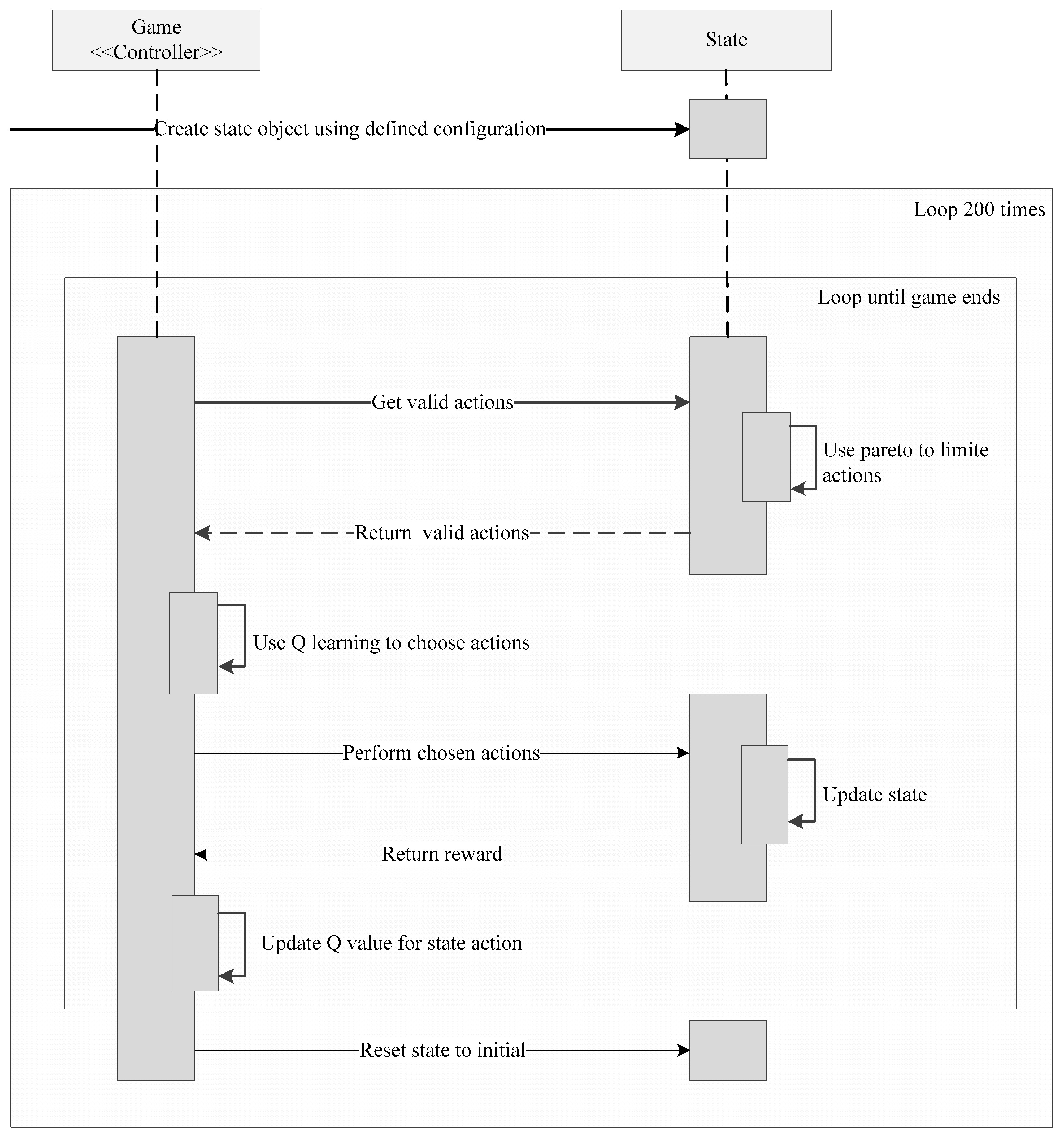
Figure 7 shows sequence diagram of the program, the program consisted of one game object acting as controller of the state object. The state object holds the current state, network definition, and logic to calculate Pareto fronts. The game object holds the logic to calculate the Q-values needed for the Q-learning.
During a single game, the game object will retrieve the valid actions from the state, use the Q-values to choose an action, update the state, and update the Q-values, until the game ends. Once the game ends, it resets the state object to the initial state and starts a new game. It repeats this 200 times.
4.4. Experiment Result Definition
Each game iteration produces a final score, which is the cumulative reward of that game. The goal of the defender, as defined in the game model section, is to maximize that cumulative reward.
Note, that the game has three separate objectives and, thus, the reward is a 3D vector. An optimal defense policy will have a higher cumulative reward than a non-optimal defense policy.
In order to resolve the stated problem statements, the results of the experiments should show that, over time, the Pareto-Q-learning approach leads to higher cumulative rewards. By mapping the cumulative rewards of games played over time, we can show just that.
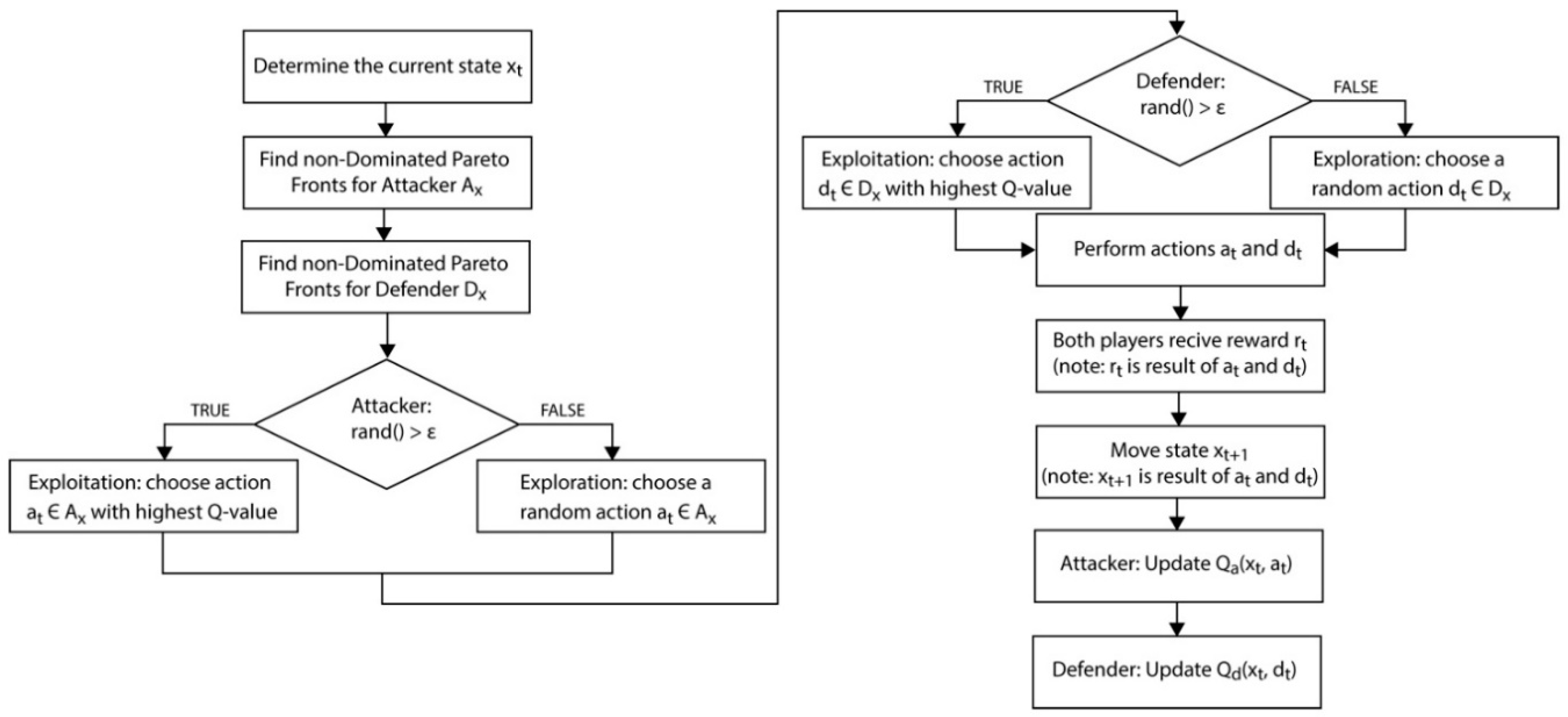
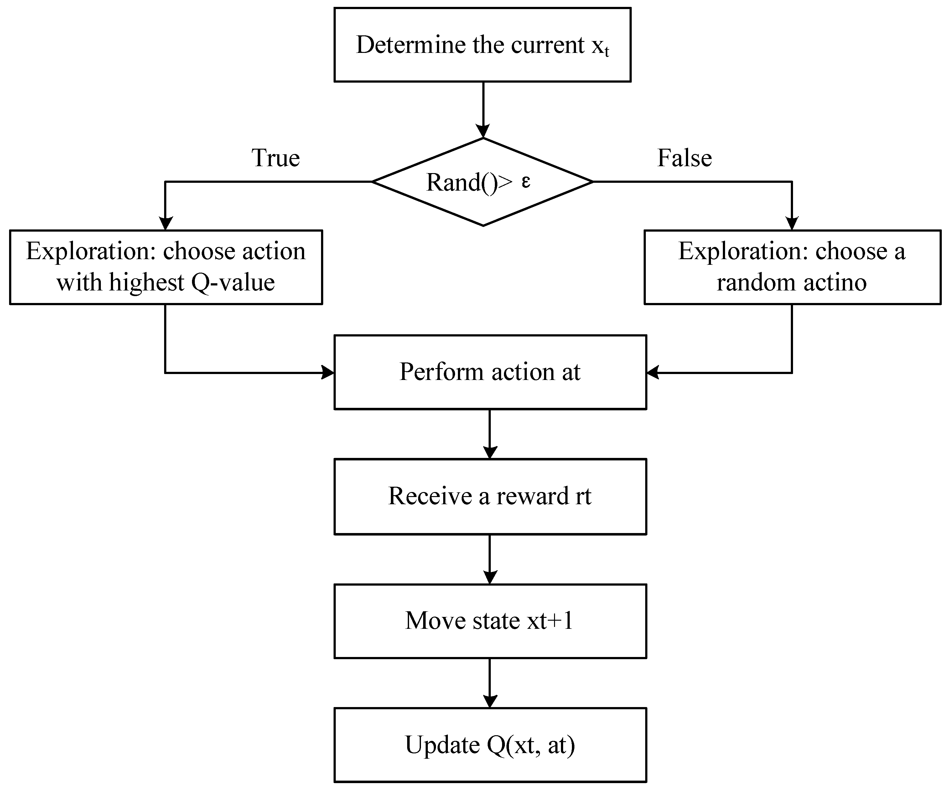
Each configuration of the game was run 200 times. The cumulative reward of each game was averaged over two iterations, creating 100 data points for analysis. The averaging to 100 points was done in order to decrease the variability between the results. While learning, the Pareto-Q-learning algorithm will, from time to time, select a random action, when rand() > ε. These random choices are a feature of Q-learning, as visible in
Figure 2 and
Figure 3, and are necessary for the exploration of the state space. However, this can lead to very different rewards and, thus, increase the variability of the results.
4.5. Pseudo-Code for Pareto-Q-Learning
This section shows the pseudo-code for the game Q-learning logic in the game object and Pareto optimization logic in the state object.
----------------------------------
Game.playGame() -→ Q-learning
----------------------------------
while ( !gameOver ) {
  state = new State(graph, points);
  // Get a map of valid actions for the given state
  ATTactionsMap <Action, reward> = attacker.getActions(state);
  DEFactionsMap <Action, reward> = defender.getActions(state);

  // Get the Non-Dominated Pareto Fronts
  ATTactionsMap <Action, reward> = paretoFrontsForAttacker();
  DEFactionsMap <Action, reward> = paretoFrontsForDefender();

  // Perform the Q-learning using the Non-Dominated Pareto Fronts
  if(rand() > epsilon){
    // Exploit the Q value for Attacker (use softmax)
    DEFaction = pickLearnedAction(state, DEFactionsMap);
  } else {
    // Explore the available actions for Attacker
    DEFaction = pickRandomAction(state, DEFactionsMap);
  }

  // Update the Q-values
  updateQvalues(state, ATTaction, DEFaction);

  // Update the graph and points objects
  gameOver = attacker.performAction(ATTaction, graph, points);
  gameOver = defender.performAction(DEFaction, graph, points) || gameOver;
}
----------------------------------
State.paretoFrontForDefender(ATTactionsMap, DEFactionsMap, state)
----------------------------------
// Group the actions by defense
foreach (defenseAction in DEFactionsMap){

  // Loop through the attacks and find the best attacks
  foreach (currentAttack in ATTactionsMap) {
    // Check if the current attack is dominated by an alternative Attack
    foreach (altAttack in ATTactionMap){
      // Note that this is a vector comparison
      if(currentAttack != altAttack && graph.calculateReward(currentAttack,
        defenseAction) <= graph.calculateReward(altAttack,defenseAction)){
          // The current Attack is dominated
          addToFront = false;
      }
}

    if(addToFront){
  paretoDEFfrontMap[defenseAction].add(currentAction,
  graph.calculateReward(currentAttack, defenseAction));
    }
  }
}

// Remove the defense actions with dominated Pareto fronts
foreach (currentDefense in paretoDEFfrontMap) {
  foreach(altDefense in paretoDEFfrontMap){
    foreach(altAttack in paretoDEFfrontMap[altDefense]){
      foreach(anyAttack in paretoDEFfrontMap[currentDefense]){
        if(!(paretoDEFfrontMap[altDefense][altAttack] <=
            paretoDEFfrontMap[currentDefense][anyAttack]){
              dominant = false;
        }
      }

      // Remove dominated Pareto fronts
      if(dominant){
        DEFactionsMap.remove(currentDefense);
      }
    }
  }
}
5. Results and Analysis
The results show cumulative rewards over time. If the Pareto-Q-learning leads to an optimal solution, the cumulative rewards should increase over time in all three dimensions. In order to validate that this is the result of the approach and not the game definition, the Pareto-Q-learning rewards should be compared to a base case of arbitrary (random) actions and a simple Q-learning approach (i.e., the possible action space is not limited by Pareto optimization).
A visual representation of the network with configuration of 100 nodes and 0.05 sparsity is given in
Figure 8,
Figure 9 and
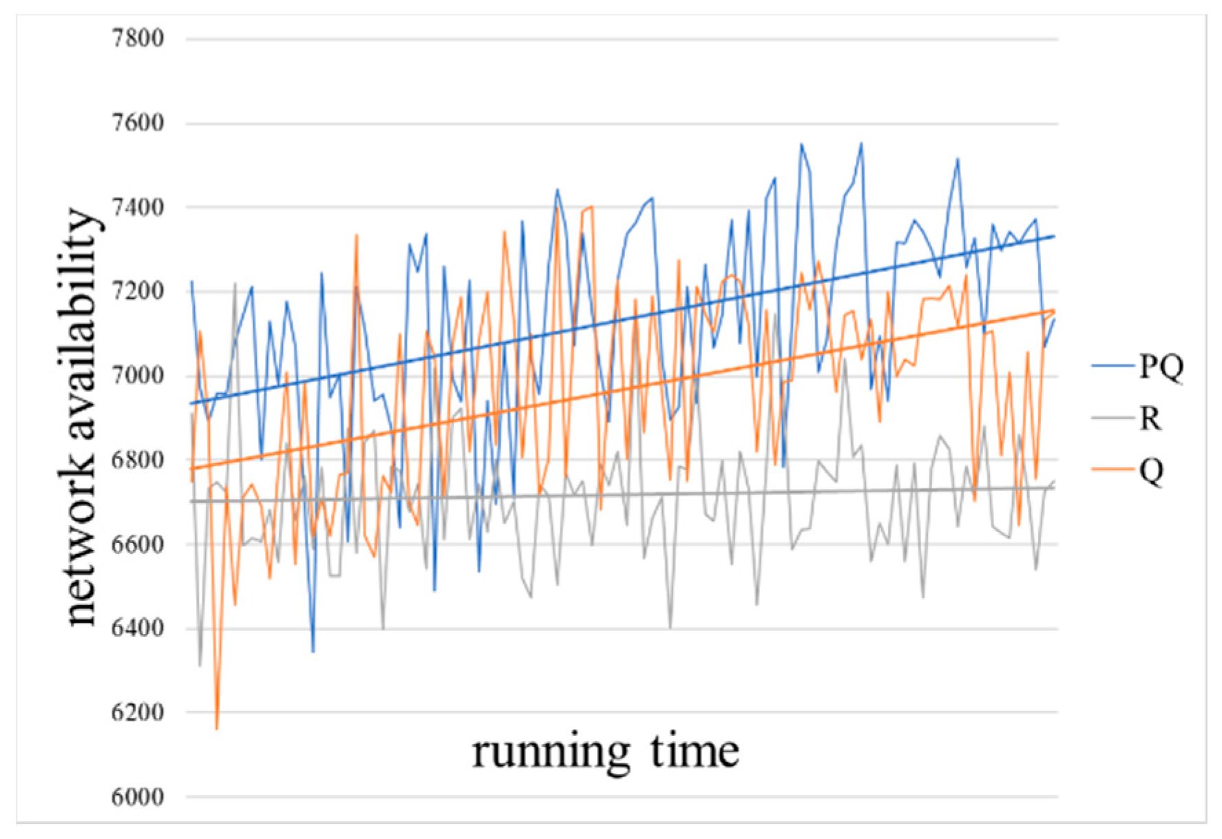
Figure 10, and the results showing improvement over time are visible.
Figure 8 shows the network availability (
),
Figure 9 shows the node security (
) over the same games, and
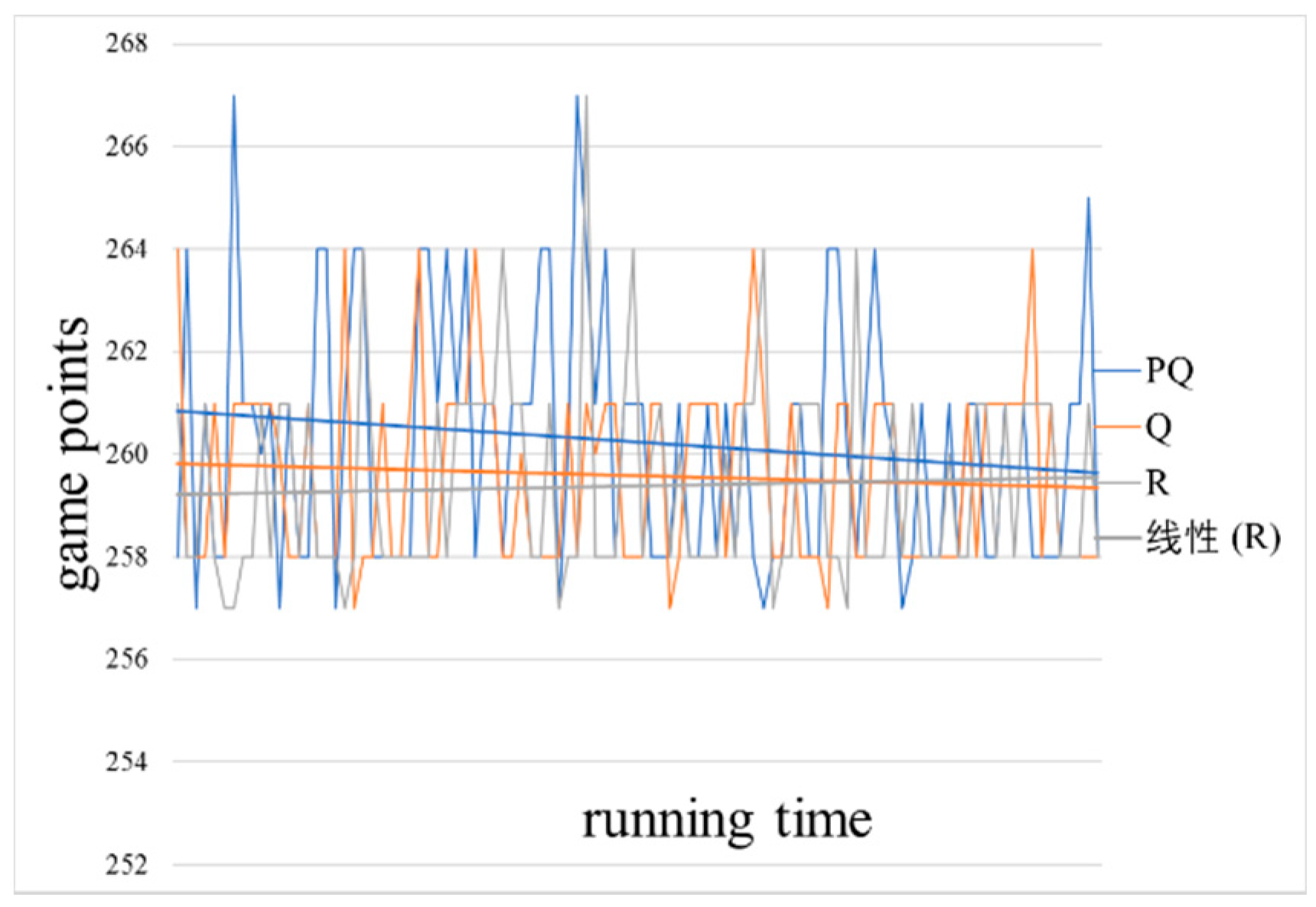
Figure 10 shows the defense strategy cost effectiveness (
) over the same games. The configuration for these figures are derived from
Table 1, reflecting 100 nodes, a sparsity of 0.05, and both the defender and attacker start with 250 game points. The weights of the nodes are randomly generation within the limits described in
Table 1.
We implemented the game using Python version 3.6 (2017) and the NumPy library (2017), Python is a free software by Python Software Foundation, America, and NumPy is the fundamental package for scientific computing with Python. The experiment was run on a MacBook Pro 2016 model machine (MacOS Sierra Version 10.12.6) with an Intel Core i5 (dual-core 3.1 GHz) CPU and 8 GB of RAM (Random-Access Memory). We use the machine’s internal SSD (Solid State Drives) hard-disk for storing data.
According to the experimental configuration in
Section 4.3, the algorithm performs 200 simulation calculations. The result is shown in
Figure 8,
Figure 9,
Figure 10 and
Figure 11, which represent the values of the game target
–
and the cumulative reward vector. As shown in
Section 4.1, the value of the cumulative reward vector is calculated based on the weights of 6:2:2 for the game targets
,
, and
, where the blue lines represent the result of the PQ (Pareto-Q-learning) algorithm, the orange are Q algorithm results and the gray are random results. In order to facilitate the comparison of different algorithms, the results are processed by a linear smoothing process, as shown by straight lines. The horizontal axis in the figures represents the time of the simulation calculation, and the vertical axis represents the corresponding game target value. The higher the data point on the straight line in the figure, the better the network availability and node security that the defender can obtain at the lower cost in the network attack and defense game.
The results clearly show that the Pareto-Q-learning algorithm outperforms both the basic Q-learning algorithm and a random baseline. In fact, you can see that the Pareto-Q-learning approach outperforms from the very first iteration. This is in contrast with the Q-learning approach which, although it slowly improves over time, it clearly gives lower rewards than the combined approach.
In
Figure 8 and
Figure 9, you can see that over time simple Q-learning does approach the results of the Pareto-Q-learning implementation. It is expected that simple Q-learning will eventually reach the same solution as the Pareto-Q-learning algorithm. The initial advantage of the Pareto-Q-learning approach means that from the beginning the results are sufficiently optimal to allow network administrators to run the algorithm for fewer iterations than they would have to when using simple Q-learning.
Both network availability () and node security () see an increase in cumulative reward. This is because the goals are completely independent. A move designed to increase the cumulative reward of the network availability has no effect on node security, and vice versa. If the goals were weighted in favor of either goal, the results would show a strong preference for one goal over the other, leading the software agent to consistently choose one goal. This would result in the other goal showing less growth.
In
Figure 10, we see that both Pareto-Q-learning and simple Q-learning actually decrease over time. We believe that is the result of the very large difference between the maintenance cost and the cost of performing an action. The high number of nodes, means the loss of game points due to performing an action, is trivial when compared to the fixed cost of maintenance. Therefore, it is generally not advantageous for the software agent to “do nothing”, which is the only action avoiding the loss of game points. Additionally, the high maintenance cost leads to games that end rather early (an average of four moves per game) and all is due to the third end condition of the game being met (see game rules: if either the attacker or the defender can no longer make a move, the game ends). Realistically, it is very unlikely for an attacker to completely bring down a network. He could steal all the data, but that would lead to much longer games and take a very long game due to: (1) a good defender stopping the attacker from ever bringing down the network/stealing all the data; (2) a good attacker has to specifically focus on stealing data, thus ignoring the other goals (and this will still take many moves, because the defender will try to stop him); and (3) a lucky attacker accidentally wins the game, which is a statistical fluke and should probably be ignored.
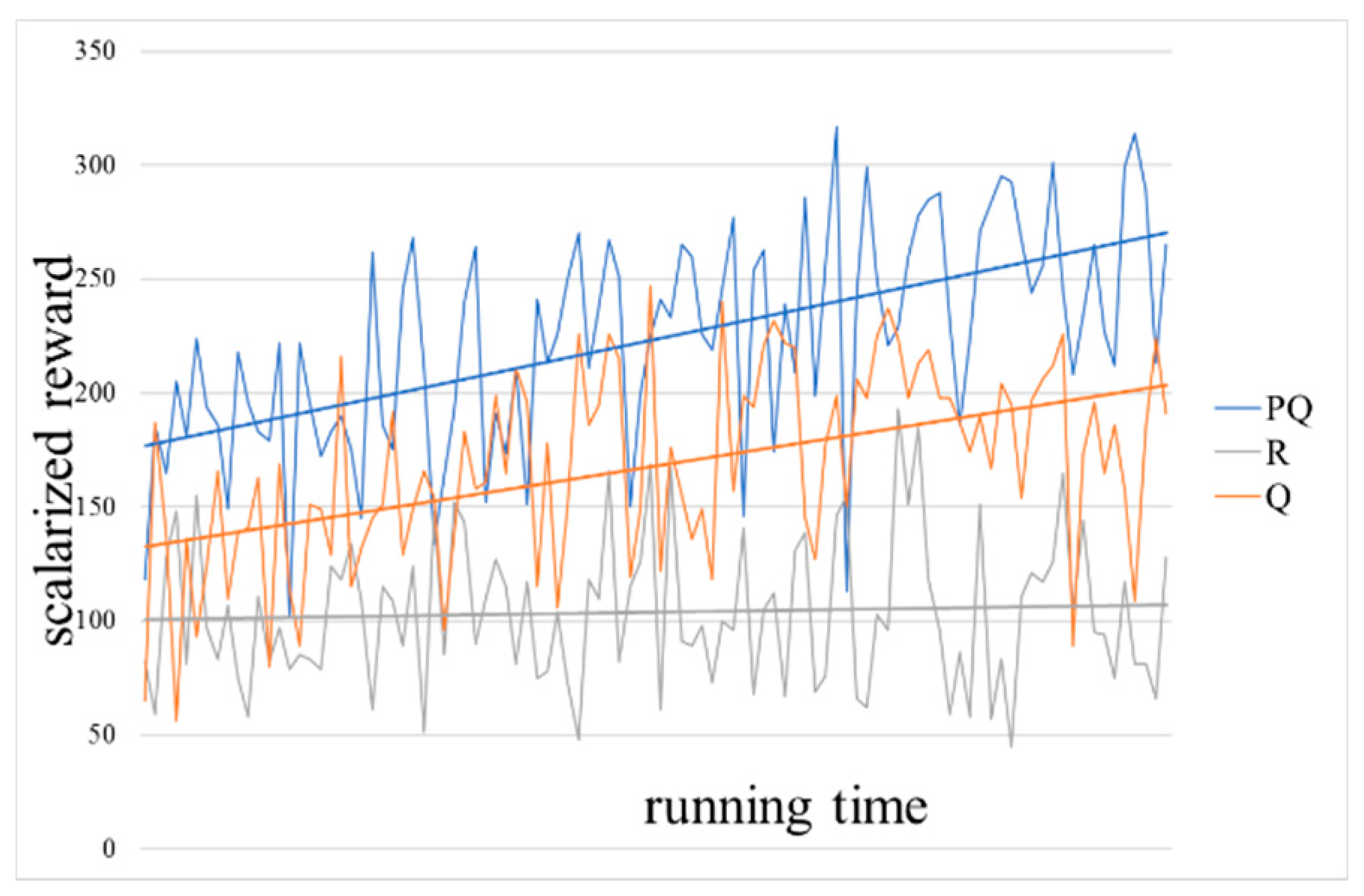
To better visualize the improvement over time, we created a normalized scalarization of the cumulative reward vector. As visible in
Figure 11, the approach clearly leads to better cumulative rewards over time. Note that the results are normalized at 100 and the arbitrary (random) strategy never strays from that base. The obvious advantage of the Pareto-Q-learning approach is especially clear in this graph. The Pareto-Q-learning approach is more than 2.5 times as effective as an arbitrary strategy. We also included a linear fit to the data to show that the results clearly increase over time. While the growth may not be exactly linear, we feel that the linear curve best visualizes the difference in results over time.
We can conclude that, if we consider the initial network state as a good condition, the Pareto-Q-learning algorithm of this paper leads to a final state with improved network performance. It reaches this state in fewer moves than a simple Q-learning or arbitrary policy, which indicates that the Pareto-Q-learning algorithm is more effective than other methods.
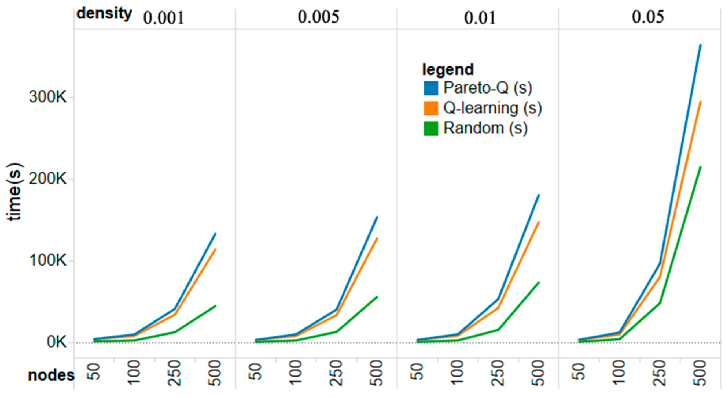
The Pareto-Q-learning approach is, unfortunately, more computationally expensive than simple Q-learning. This is understandable as it is a combination of the two methods and, therefore, requires the calculation of Pareto fronts on top of the full computation of the regular Q-learning. A comparison between execution times in seconds is given in
Figure 12. Our implementation of the Pareto algorithm leads to greater execution time in large action spaces. However, increasing the efficiency of the Pareto algorithm is not the goal of this paper. Moreover, a shorter number of games matches the actual situation, and is conducive to the defenders to prevent attacks as soon as possible in the practical application. Instead we focus on the number of game moves that it takes to come to an optimal strategy instead of the actual running time.
We believe that the immediate outperformance of the Pareto-Q-learning algorithm is due to the elimination of clearly inferior actions from the set of possible actions that the Q-learning algorithm can explore. The result is a rapid determination of an optimal defense strategy.
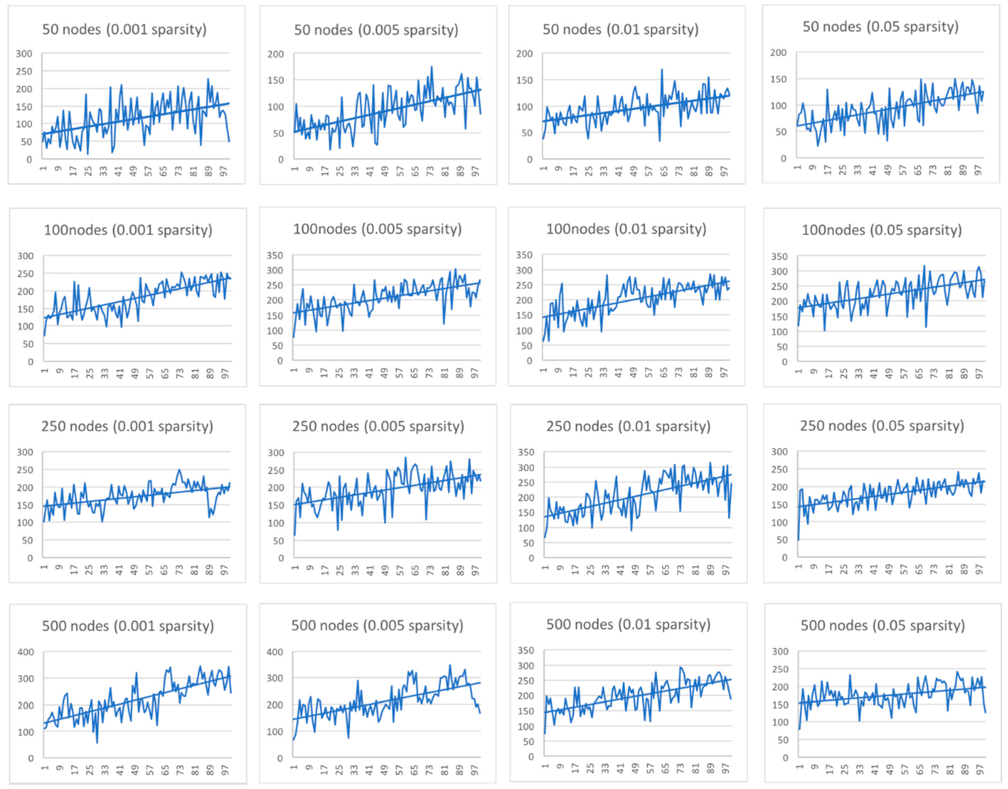
To determine if the approach works in different network conditions, we graphed the scalarized cumulative reward vector over time for the 16 different configurations described in the experiment planning section. The horizontal axis represents the running time in the corresponding network configuration, and the vertical axis represents the corresponding cumulative reward function value; the higher the reward function value, the better the game result.
Figure 13 shows that for each implemented configuration the Pareto-Q-learning approach leads to an increase in the cumulative reward over time.
One disadvantage of the Pareto-Q-learning approach, is that it does not completely solve the problem of a large action space. As is visible from
Figure 13, an increase in either the sparsity or the number (i.e., increasing the action space) does effectively decrease the learn rate. The Pareto-Q-learning approach, as an improvement of simple Q-learning, will eventually encounter the same problems as Q-learning in terms of problems with a large action space.
Another disadvantage is the high variance in strategy selection. We believe that is the result of the stochastic nature of Q-learning in the exploration phase. By randomly selecting strategies, the results vary wildly. The independent nature of the goals exacerbates this problem, as an accidental move that highly rewards one goal may lead to a policy that pursues that goal at cost of the others. This is visible in the uniform distribution ignoring the “do-nothing” strategy, which has a low chance of being selected from the very large action space.
6. Conclusions and Future Work
In this article, we presented an application of reinforcement learning, specifically Q-learning, to determine an optimal defense policy for computer networks. We enhanced the basic Q-learning approach by expanding it to multiple objectives and pre-screening possible actions with Pareto optimization. The results of our experiment show that basic Q-learning is a slow approach for network security analysis, but the process can be made significantly more efficient by applying Pareto optimization to the defense strategy selection process.
The work presented in this paper has several limitations. Our game model consists of nodes, which are directly connected to each other. However, most real-world networks have various devices that facilitates connection between devices such as routers and switches. In addition to that, in our model the attacker chooses random actions. In real computer networks, attackers do not behave in this way. Even if the attacker, blinded, performs random attacks at the beginning, he will change his strategy over time. Therefore, it seems difficult to use these approaches to counteract a real-time attack. The model does not consider that the attacker has a defined goal, nor do we explicitly predict attacker behavior. Instead, we merely focus on the defender.
We feel that the presented experiment functions best as an academic exercise, which shows the advantages offered by combining Pareto optimization and reinforcement learning. The method can be used for systematic monitoring of a network or a set of computers. Network defenders can run an offline system analysis based on the model, and use the results as a reference for planning defense strategies. This is especially useful for networks with a large number of nodes.
While the current model provides us with an automated defense selection mechanism, we can see that the results were still plagued by a rather high variance in the game scores. As indicated in the results analysis, we assume this to be the result of the algorithm’s inability to balance the divergent goals. We suggest that future work be focused on choosing an optimal strategy from independent, and seemingly equally important, goals and applying that to Pareto set domination.
Another direction for future work, is implementing this approach for an information system facing an emulated distributed denial of service attack. We can test, independently of the processor time delay, the propagation of the attack and of the reaction of the defender.


