Bio-Inspired Real-Time Prediction of Human Locomotion for Exoskeletal Robot Control

Abstract

Human motion detection is of fundamental importance for control of human–robot coupled systems such as exoskeletal robots. Inertial measurement units have been widely used for this purpose, although delay is a major challenge for inertial measurement unit-based motion capture systems. In this paper, we use previous and current inertial measurement unit readings to predict human locomotion based on their kinematic properties. Human locomotion is a synergetic process of the musculoskeletal system characterized by smoothness, high nonlinearity, and quasi-periodicity. Takens’ reconstruction method can well characterize quasi-periodicity and nonlinear systems. With Takens’ reconstruction framework, we developed improving methods, including Gaussian coefficient weighting and offset correction (which is based on the smoothness of human locomotion), Kalman fusion with complementary joint data prediction and united source of historical embedding generation (which is synergy-inspired), and Kalman fusion with the Newton-based method with a velocity and acceleration high-gain observer (also based on smoothness). After thorough analysis of the parameters and the effect of these improving techniques, we propose a novel prediction method that possesses the combined advantages of parameter robustness, high accuracy, trajectory smoothness, zero dead time, and adaptability to irregularities. The proposed methods were tested and validated by experiments, and the real-time applicability in a human locomotion capture system was also validated.

1. Introduction

Human motion detection is of fundamental importance for control of human–robot coupled systems such as exoskeletal robots, and for many other applications. In recent years, inertial measurement unit (IMU) technologies have quickly evolved, and complex mechanisms for tracking the operator’s movement [1,2] have gradually been replaced by motion capture systems comprising IMUs [3,4,5,6,7]. IMU-based motion capture systems have unique advantages, such as multidimensional information richness, compactness, and light weight. However, compared with biosensors for which signals appears earlier than in human body motion [8,9,10], human motion capture systems bear the apparent disadvantage of asynchronization with execution delay, which is a critical challenge for applications in exoskeletal robot control.

Human locomotion is a nonlinear quasi-periodic process with chaos [11] resulting from latent human musculoskeletal dynamics. During human walking, the two lower limbs operate synergistically [12,13,14,15]. Both the quasi-periodicity and the synergy lead to the development of several efficient prediction methods. Firstly, by drawing evidence from the lower limb synergy, echo control has long been used in powered prosthesis for generating joint trajectories of one limb by a phase shift of the opposite limb [16]. To apply echo control in prediction, the time shift needs to be correctly identified. Secondly, the complementary limb motion estimation (CLME) method [8] improves the echo control method by assuming a coupling relationship between the two lower limbs. However, its performance is not always consistent due to a significant influence from the underlying regression method [17]. Thirdly, the aforementioned quasi-periodic nonlinear behaviour of walking has led to Takens’ reconstruction method, which is closely related to Takens’ reconstruction theorem. It is essentially a nonlinear time series dynamic factor analysis method for predicting joint trajectories [18,19]. However, it requires historical system data to achieve a better performance which brings in inevitable dead time. There are also some other prediction methods, such as the autoregressive integrated model method, autoregressive integrated moving average method, autoregressive moving average model method [20], and modified recursive least square methods [21], which are also time series analysis methods but with undesired computational expense, dead time, or complex parameter tuning processes. Besides, the consistency and smoothness of human joint motion should not be ignored as human joints possess apparent biological damping [22,23,24] which damps out the high frequency vibration. Such observations indicate that the traditional Newton’s method, in the short term for smoothing or correction techniques, might be beneficial. For Newton’s method, estimation of the velocity and acceleration with noise rejecting ability is needed. High-gain observers could be exploited, which are usually used in robot or automation applications [25,26,27].

In this work, we consider, without loss of generality, a series of prediction methods and its improving techniques utilizing the biological features of human locomotion. Based on progressive analysis, we introduce a novel method which fuses the advantages of different approaches to achieve an even better performance verified by a daily motion dataset of a normal subject, including irregular motion. The method is also applicable to real-time embedded systems.

This paper is organized as follows. Section 2 introduces the IMU-based motion capture system. Section 3 describes different prediction methods, assessment measures, and the used dataset. Section 4 evaluates the influence of several common parameters and the prediction performance with different prediction methods by simulation, elaborates their characteristics, and then proposes our best method. Also, the real-time applicability of the proposed algorithm is demonstrated. Section 5 concludes the paper.

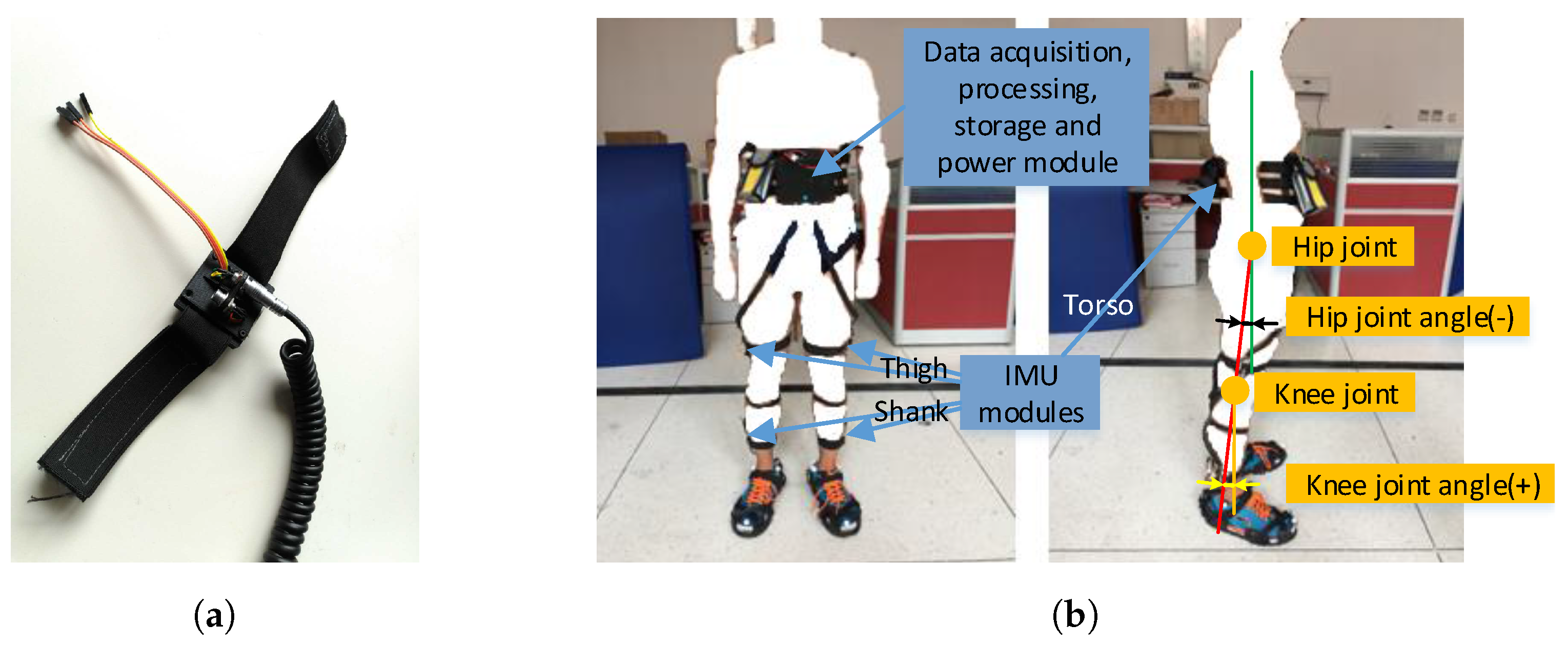
2. The IMU-Based Motion Capture System

A motion capture system using IMUs has been developed by Xeno Dynamics Co., Ltd. (Shenzhen, Guangdong, China), as shown in Figure 1. In each IMU, the gyroscope, accelerometer and magnetometer data are fused with a gradient descent algorithm with magnetic distortion compensation [28]. The compact rigid container with elastic straps could be easily attached to human lower limbs. The data collected by serial communication could either be stored and processed in a standalone central control device as shown in Figure 1b or sent into the developing exoskeletal robots with a sampling frequency of 50 Hz. The test subject can move freely when wearing the motion capture system. In the experiment designed in this research, only the left hip, right hip, left knee, and right knee joint data in the human sagittal plane were collected, as illustrated in Figure 1b.

3. Methods

The prediction methods starts with Takens’ reconstruction prediction and its enhancement with Gaussian coefficient weighting, offset correction, and a feedback scheme. Synergy of a complementary joint is exploited with two methods producing the synergy-enhanced Takens’ reconstruction predictions. To further improve the prediction performance during the short term, and adaptability to irregularities, the classic Newton’s method with a high-gain observer is brought in and some new methods appear.

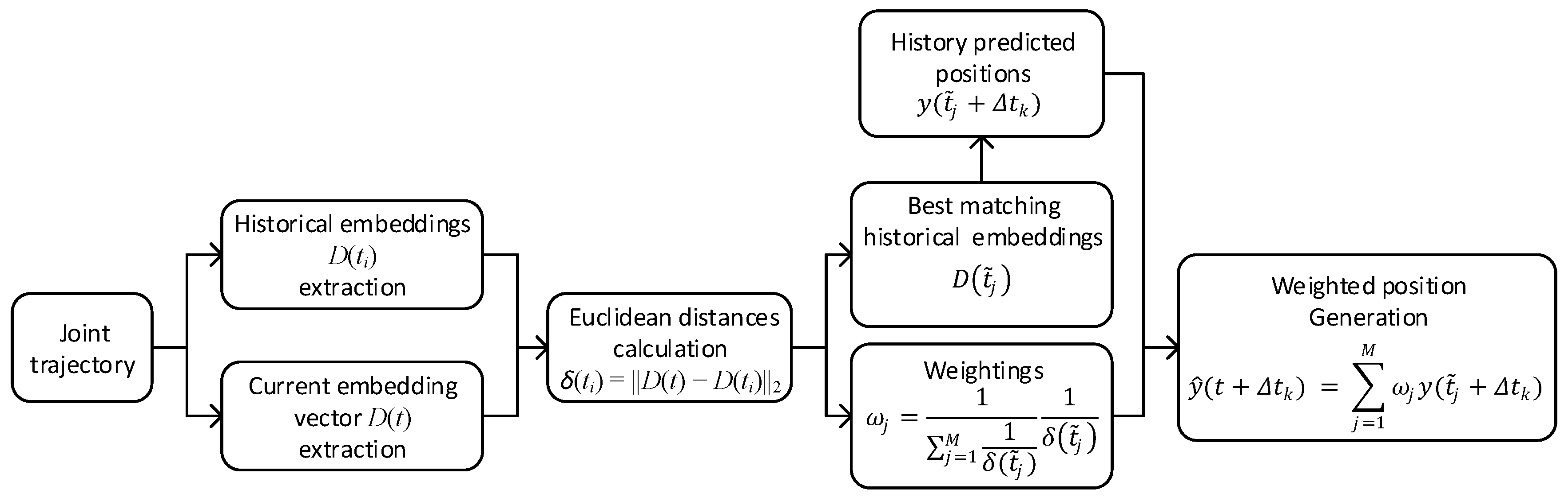
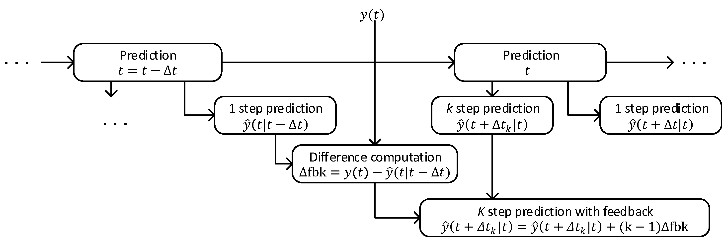
3.1. Takens’ Reconstruction Prediction and Modifications Based on Motion Smoothness

Takens’ reconstruction method is correct for predicting the joint trajectories of human lower limbs, which present quasi-periodicity and nonlinearity. According to Takens’ reconstruction theorem, it is possible to reconstruct the dynamics of a nonlinear system based on its past measurements. For this purpose, a current embedding vector is defined:

$$D\left(t\right)={\left[\begin{array}{cccc}y\left(t\right)& y(t-\Delta t)& \cdots & y(t-(p-1)\Delta t)\end{array}\right]}^T,$$

(1)

where $y\left(t\right)$ stands for the current state which might be position, velocity, acceleration, etc., t is the current sampling instant, p is the embedding vector length, and the sampling constant is $\Delta t$. Takens’ original reconstruction algorithm proposed by Herrmann [19] is illustrated in Figure 2:

At each sampling instant t with $t\ge l\Delta t$, an embedding vector $D\left(t\right)$ is acquired. The current embedding vector $D\left(t\right)$ is then compared to all collected historical embeddings $D\left(t_i\right)$ with $l\Delta t\le t_i<t$ by determining the Euclidean distances

$$\delta \left(i\right)=\sqrt{\sum _{x=1}^p{(y(t_i-\Delta t_{x-1})-y(t-\Delta t_{x-1}))}^2},$$

(2)

In Equation (2) i is the index of the ith historical embedding $D\left(t_i\right)$ and $1\le i\le l$. l is also called the history data length. As $D\left(t_i\right)$ is a vector composed of a series of states, the first component of $D\left(t_i\right)$ is labeled as $y\left(t_i\right)$ and the components are defined as $y(t_i-\Delta t_{x-1})$ where $\Delta t_{x-1}=(x-1)\Delta t$ and $1\le x\le p$.

The M best matching embeddings $D\left({\tilde{t}}_1\right),D\left({\tilde{t}}_2\right),\dots ,D\left({\tilde{t}}_M\right)$ from the sampling instants ${\tilde{t}}_j$ with $1\le j\le M$ are used to calculate a k-step prediction $\widehat{y}(t+\Delta t_k|t)$:

$$\widehat{y}(t+\Delta t_k|t)=\sum _{j=1}^M{\omega }_{j}y({\tilde{t}}_j+\Delta t_k),$$

(3)

with the weightings

$${\omega }_j=\frac{1}{N}\frac{1}{\delta \left({\tilde{t}}_j\right)},$$

(4)

and

$$N=\sum _{j=1}^M\frac{1}{\delta \left({\tilde{t}}_j\right)},$$

(5)

In Equation (3) $\Delta t_k=k\Delta t$. When k = 1, the subscript is dropped as $\Delta t$. k is also called prediction horizon.

Although Takens’ reconstruction method bears many practical advantages such as easy parameter calibration, result smoothness, accuracy and so on, its improvement is still quite possible. The natural smoothness of motion brought by the human body indicates whether high frequency jumps and sharp spikes in trajectories were initially predicted, as correction and smoothing techniques would be used to produce a more realistic result.

First, we assumed that the $y(t_i-\Delta t_{x-1})$ in $D\left(t_i\right)$ closer to $y\left(t_i\right)$ had more of an influence on Euclidean distance determination. Thus, the Euclidean distances was calculated with the addition of Gaussian coefficients $G\left(x\right)$:

$$\delta \left(i\right)=\sqrt{\sum _{x=1}^p{\left((y(t_i-\Delta t_{x-1})-y(t-\Delta t_{x-1}))G\left(x\right)\right)}^2},$$

(6)

and

$$G\left(x\right)=e^{-\frac{1}{2}{(\frac{x-1}{\frac{Q}{p}})}^2},$$

(7)

where Q is constant and p is the embedding vector length. As the prediction result was not very sensitive to the value of Q, it was chosen to be 4 in this research, which was justified by several items of gait data.

Second, the offset between $y\left({\tilde{t}}_j\right)$ in a best matching embedding of $D\left({\tilde{t}}_j\right)$ and $y\left(t\right)$ in the current embedding vector was decided during each vector match by

$$\Delta y_j=y\left({\tilde{t}}_j\right)-y\left(t\right),$$

(8)

where $y\left({\tilde{t}}_j\right)$ means the past observation of the current state $y\left(t\right)$ in the jth best matching vector $D\left({\tilde{t}}_j\right)$. The obtained $\Delta y_j$ is used for correction during the weighting procedure with the equation

$$\widehat{y}(t+\Delta t_k|t)=\sum _{j=1}^M{\omega }_j\left(y({\tilde{t}}_j+\Delta t_k)-\Delta y_j\right),$$

(9)

Third, the feedback scheme is integrated and tested as illustrated in Figure 3.

At time t, the 1 step prediction $\widehat{y}\left(t\right|t-\Delta t)$ of the current time is achieved at $t-\Delta t$. The difference between the current position $y\left(t\right)$ and $\widehat{y}\left(t\right|t-\Delta t)$, $\Delta fbk$, is added to the current k step prediction $\widehat{y}(t+\Delta t_k|t)$ with a factor of $k-1$. At the same time a new 1 step prediction is completed as $\widehat{y}(t+\Delta t|t)$, which will be used in the feedback determination in the next time step.

3.2. Takens’ Reconstruction Method’s Synergy Improvement

The synergy feature of the lower limb joints could be used in a simple way for Takens’ reconstruction-based methods, making use of the complementary joint motion data of the other limb. Basically, considering the complementary joint data as another source of history or taking it as an indirect measurement of the original joint motion should be able to provide help. This results in two distinct methods:

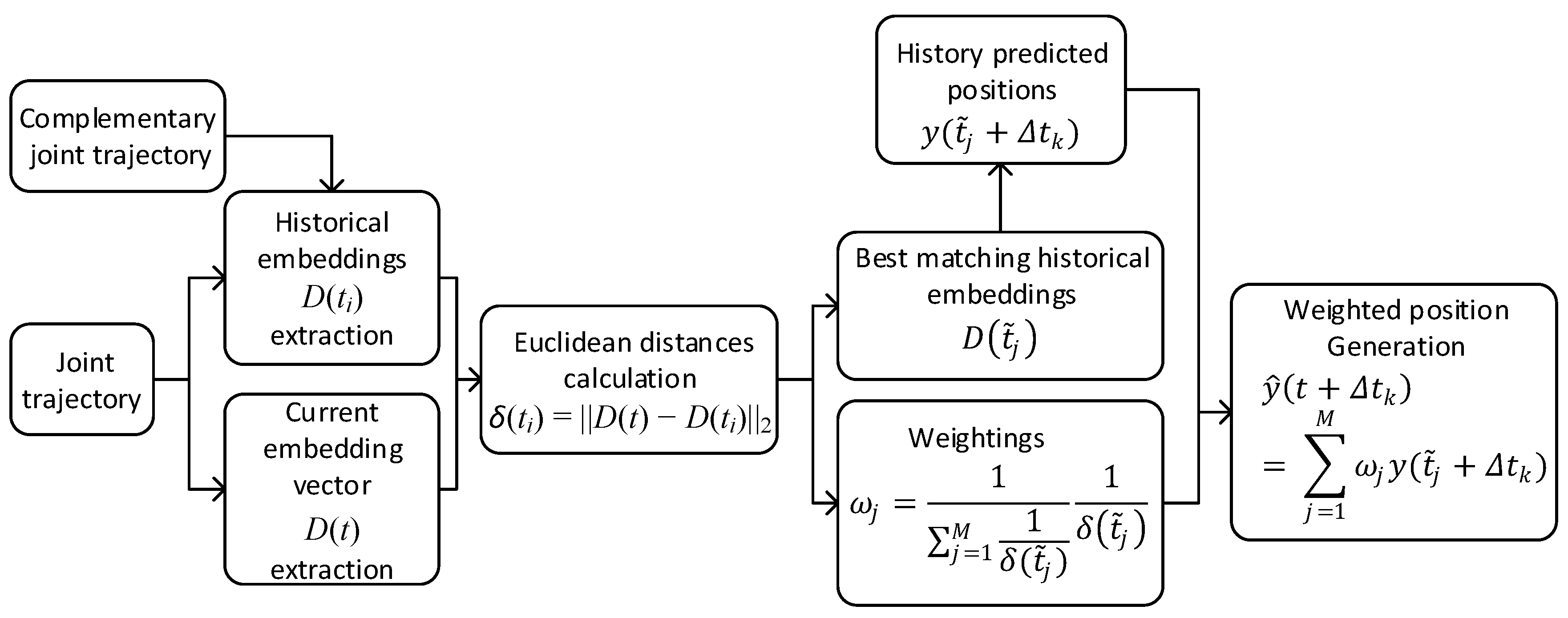
• While searching for the best matching vectors, the embedding vectors are generated with the united source of the two joints’ history data. The detailed process is shown in Figure 4.
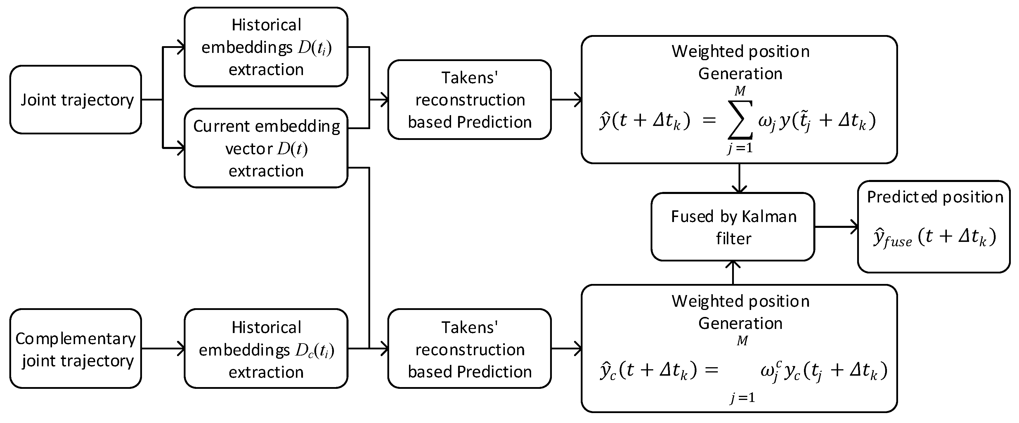
• Predict k step position ahead as usual and get $\widehat{y}(t+\Delta t_k|t)$. Then take the complementary joint as the source of embedding vector generation and predict ${\widehat{y}}_c(t+\Delta t_k|t)$. Finally, fuse $\widehat{y}(t+\Delta t_k|t)$ and ${\widehat{y}}_c(t+\Delta t_k|t)$ with the Kalman filter and obtain ${\widehat{y}}_{fuse}(t+\Delta t_k|t)$. The detailed process is shown in Figure 5.

The two means represented different directions. They have limited theoretical foundation as the synergy mechanism is still under research and could not be commented by comparative analysis without being applied to assessment on real data.

3.3. Takens’ Reconstruction Adaptability Enhancement with Newton’s Method

Motion smoothness also means the assumption of local linearity is appropriate, thus the traditional Newton’s method in the short term might be beneficial. A high-gain observer [25,26,27] is formulated to obtain the required velocity and acceleration for a second-order Newton’s method.

$$y_{NHgo}(t+\Delta t_k|t)=y\left(t\right)+\widehat{\dot{y}}\left(t\right)\Delta t_{k+1}+\frac{1}{2}\widehat{\ddot{y}}\left(t\right)\Delta t_{k+1}^2,$$

(10)

where $\widehat{\dot{y}}$ and $\widehat{\ddot{y}}$ are computed with

$$\widehat{\dot{y}}=\frac{ϵs}{\frac{{ϵ}^3{s}^2}{{\alpha }_2}+\frac{{\alpha }_1{ϵ}^{2}s}{{\alpha }_2}+ϵ}y,$$

(11)

and

$$\widehat{\ddot{y}}=\frac{ϵs}{\frac{{ϵ}^3{s}^2}{{\alpha }_2}+\frac{{\alpha }_1{ϵ}^{2}s}{{\alpha }_2}+ϵ}\widehat{\dot{y}},$$

(12)

where ${\alpha }_1$ = 100, ${\alpha }_2$ = 80 and $ϵ$ = sampling constant which was 0.02 s in this context.

As a high-gain observer could be taken as a non-linear filter, ${\alpha }_1$ and ${\alpha }_2$ were chosen so that the amplitude of the data after the filter did not change and the phase delay in time domain was constant. It usually brought in a delay of about one sampling cycle. Equation (10) roughly compensates the delay by taking a one step longer prediction at $k+1$ as the k step result. Finally, the Newton-based and Takens’ reconstruction-based methods could be fused to achieve some methods with unique adaptability enhancement.

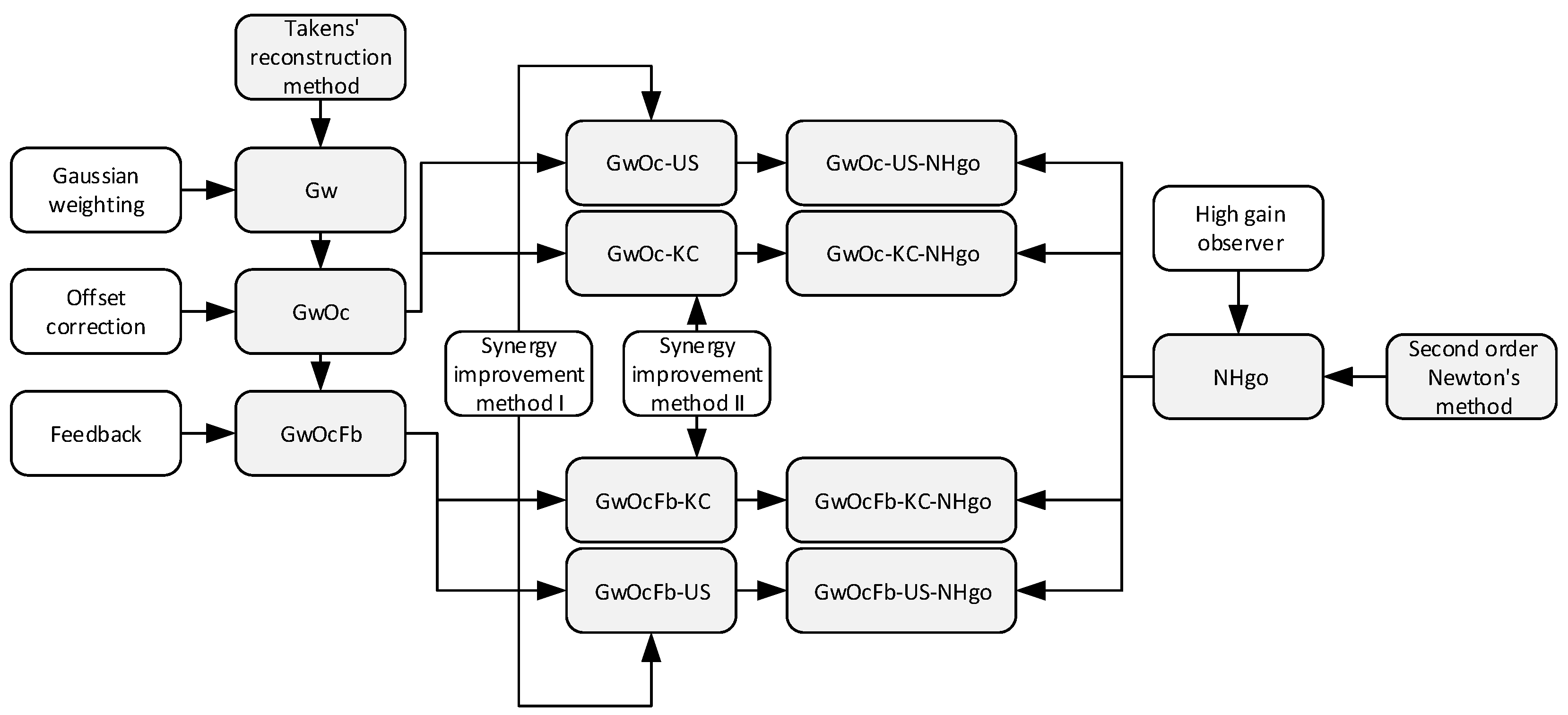
3.4. Methods Summary

Summarizing the above methods, besides the fundamental Takens’ reconstruction and Newton’s method, there are 12 new prediction methods that are introduced and analysed which are listed in

Table 1. Prediction methods in this article and their abbreviations.

Abbreviation	Method Description	Proposed by Author
Takens’	Takens’ reconstruction method	No
NHgo	Newton’s method with velocity and acceleration observed by high gain observer	Yes
Gw	Takens’ reconstruction with Gaussian weightings	Yes
GwOc	Takens’ reconstruction with Gaussian weightings and offset correction scheme	Yes
GwOcFb	Takens’ reconstruction with Gaussian weightings, offset correction and feedback scheme	Yes
GwOcFb-KC	GwOcFb predicted result Kalman fusion with the complementary joint GwOcFb predicted	Yes
GwOcFb-US	GwOcFb with coupled joints’ united source of historical embedding generation	Yes
GwOc-KC	GwOc predicted result Kalman fusion with the complementary joint GwOc-KC predicted	Yes
GwOc-US	GwOc with coupled joints’ united source of historical embedding generation	Yes
GwOcFb-US-NHgo	GwOcFb-US predicted result Kalman fusion with the NHgo predicted	Yes
GwOc-US-NHgo	GwOcFb predicted result Kalman fusion with the NHgo predicted	Yes
GwOcFb-KC-NHgo	GwOcFb-KC predicted result Kalman fusion with the NHgo predicted	Yes
GwOc-KC-NHgo	GwOc-KC predicted result Kalman fusion with the NHgo predicted	Yes

.

The relationship between different prediction methods with different improving approaches is illustrated in Figure 6.

3.5. Assessment Data

The dataset used to assess the performance of different prediction methods is 208.5 s long with a sampling rate of 50 Hz, including the joint angles of the knees and hips of a test subject in a sagittal plane. It is comprised of the following continuous motion process segmented and highlighted in Figure 7: 5 stand–sits, 5 steps walking, 2 left turns, 5 steps walking, 2 left turns, 5 steps walking, stepping onto a treadmill, 1 km/h, 2 km/h and 3 km/h walking on a treadmill, stopping and leaving the treadmill, 5 steps walking and sitting down. In order to assess the adaptability of different methods the following segments were defined as irregularities: stand–walk transition, turns, stepping on a treadmill, stopping and leaving the treadmill, and stand–sit.

3.6. Assessment Measures

To quantitatively evaluate the algorithms’ prediction performance, the prediction ratio ($PR$) representing prediction errors, and the smoothness factor ($SF$) measuring predicted trajectory smoothness are calculated by the following equations [19]:

$$PR(y\left(t\right),e\left(t\right))=1-\frac{RMS\left(e_{PR}\left(t\right)\right)}{RMS\left(y\right(t\left)\right)}\times 100\%,$$

(13)

$$e_{PR}\left(t\right)=\widehat{y}\left(t\right|t-\Delta t_k)-y\left(t\right),$$

(14)

where $\widehat{y}\left(t\right|t-\Delta t_k)$ represents the predicted current position $\widehat{y}\left(t\right)$ at $t-\Delta t_k$, which is obtained by shifting the predicted results with $\Delta t_k$ and

$$SF\left(\widehat{y}\left(t\right)\right)=\frac{1}{t_{End}(max\left(\widehat{y}\left(t\right)\right)-min\left(\widehat{y}\left(t\right)\right)}{\int }_0^{t_{End}}|f\left(t\right)-\widehat{y}\left(t\right)|,$$

(15)

where $t_{End}$ is the time when prediction ends and $f\left(t\right)$ is the filtered result of $y\left(t\right)$ by a zero-phase filter with a cut-off frequency of 5 Hz.

A higher $PR$ value means higher accuracy, while a lower $SF$ value means smoother motion. In order to provide an overall relative comparison among different methods, $PR$ and $SF$ are combined into an overall performance index ($OPI$), which is computed with

$$OPI=\alpha PR\left(i\right)/max\left(PR\right(i\left)\right)+(1-\alpha )min\left(SF\right(i\left)\right)/SF\left(i\right),$$

(16)

where i represents the index of a specific method involved in the comparison. It should be emphasized that such an index is not an absolute criterion but a relative one. The preference over prediction accuracy and smoothness could be modified by the coefficient $\alpha$.

In addition, the adaptability of prediction methods to irregularities happening from time to time is very essential. Such capability could be assessed by isolating the irregularities, including the beginning and termination of walking and the transition between different motion speed and modes.

4. Implementation and Assessment

In practical applications, prediction horizon may change in real-time, so a good algorithm does not only perform well at a fixed prediction horizon, but also over a certain range. Before the performance evaluation over different prediction horizons, the common parameters used in Takens’ reconstruction-based algorithms must be reasonably selected.

4.1. Parameter Selection for Takens’ Reconstruction-Based Methods

For Takens’ reconstruction-based methods common parameters were evaluated, including the history data length, embedding vector length, and the number of weighted best matching vectors. A group of basic parameters are listed in

Table 2. Basic parameters for parameter evaluation.

Parameter Name	Symbol	Value	Variation Range	Variable
History data length	l	360	200–400	Yes
Embedding vector length	p	20	6–20	Yes
Number of weighted best matching vectors	M	5	1–8	Yes
Prediction horizon	k	5	/	No

. During the evaluation the evaluated parameters were taken as variables while others were fixed.

Only the left hip data were shown in the following paragraphs because the four joints results exhibited the same varying patterns which meant the ruling laws were the same for different methods.

Theoretically, a longer history is beneficial and Figure 8 gave the proof with continuous escalation of $PR$s. A steep rise ended at the value of 360, which was the chosen value in Table 2. The history data length had limited influence on $SF$s after 360, because a longer history could not generate better historical embedding vectors.

The length of embedding vectors represents the orders of the reconstructed system. Excessive higher order might cause overfitting, which reduces the prediction accuracy and increases unnecessary computational expense. Gaussian weightings mitigate the problem by reducing the influence of the history data far away and the offset correction and feedback scheme also provide powerful fixation. Figure 9 proved the analysis. For the $SF$ values, the expending of embedding vectors could improve them more or less for all methods. Thus, considering that a length of 20 is not an burden to the embedded system and it has limited influence on most of the improved methods, the embedded vector length was chosen to be 20.

As shown in Figure 10, when the weighted best matching vector number increased, the $PR$s of different methods rose to the highest at 5 and the trend then descended afterwards. Meanwhile, for the $FS$s after 5, they also entered an slow falling state. This was reasonable because the matched vector quality degraded when the number increased to a certain level, and their weighting values fell quickly. At the same time, the increasing number of weighted history embedding vectors worked as a smoother by averaging down the oscillations.

Surprisingly, most newly-introduced Takens’ reconstruction-based methods exhibited robust performance with parameter variation. Thus, the parameter robustness of the newly introduced methods was discovered.

Summarizing the previous analysis, the basic parameters are selected with enough confidence, and could be applied to algorithm performance assessment.

4.2. Results and Assessment

The prediction methods listed in Table 1 and evaluated (Figure 7) demonstrated the dataset with respect to an extending prediction horizon from 1 to 20, which was the requirement of exoskeletal robot sensing for control. For $OPI$ calculation, $\alpha$ in Equation (16) was chosen as 0.8, which emphasized accuracy over smoothness. The evaluations were performed with the simulation of real-time operation by pushing the data one by one in a time sequence into the last position of a data pool, which was fair for all the methods.

Studying the results by comparison the pros and cons of different methods and improving techniques were clear:

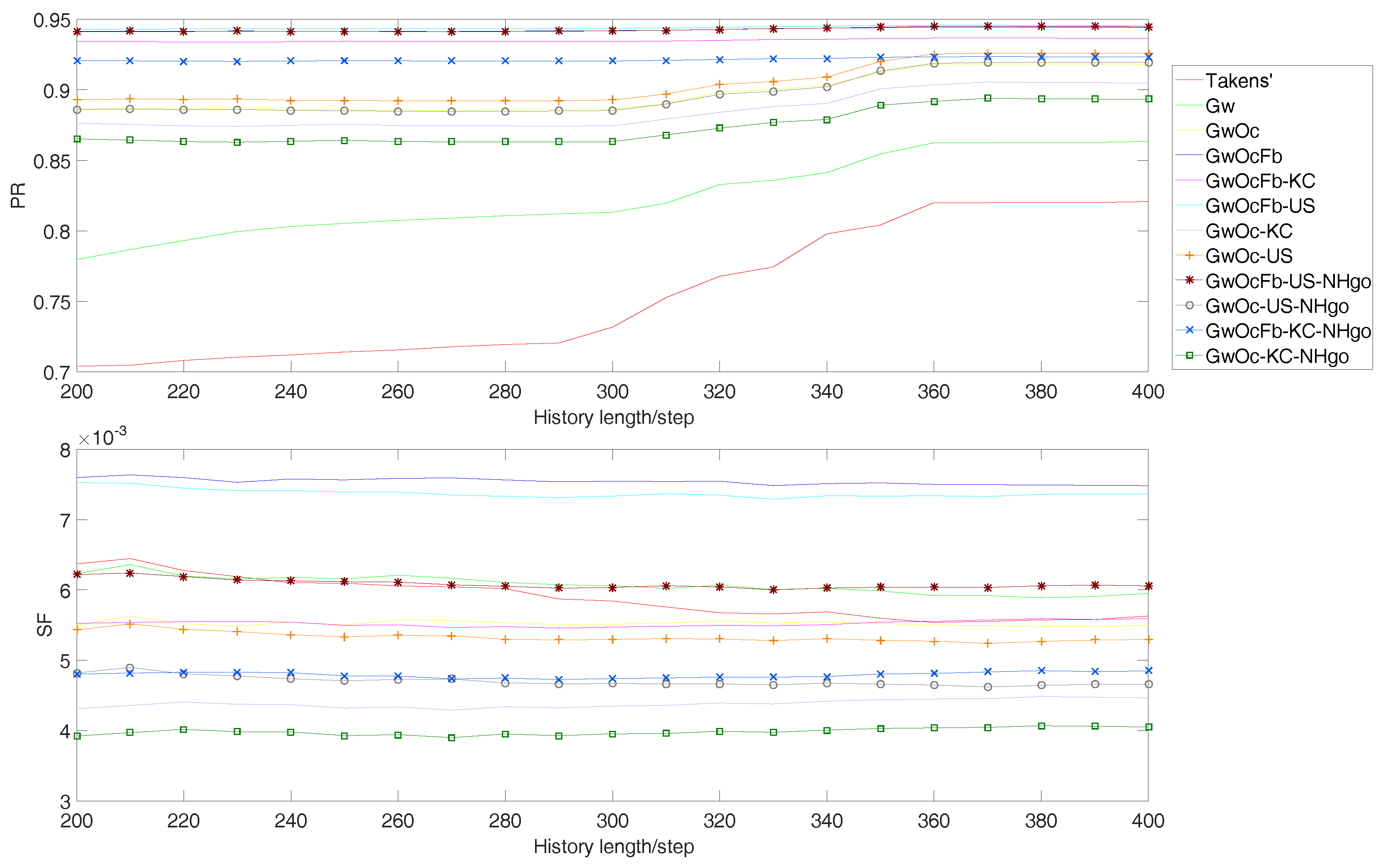
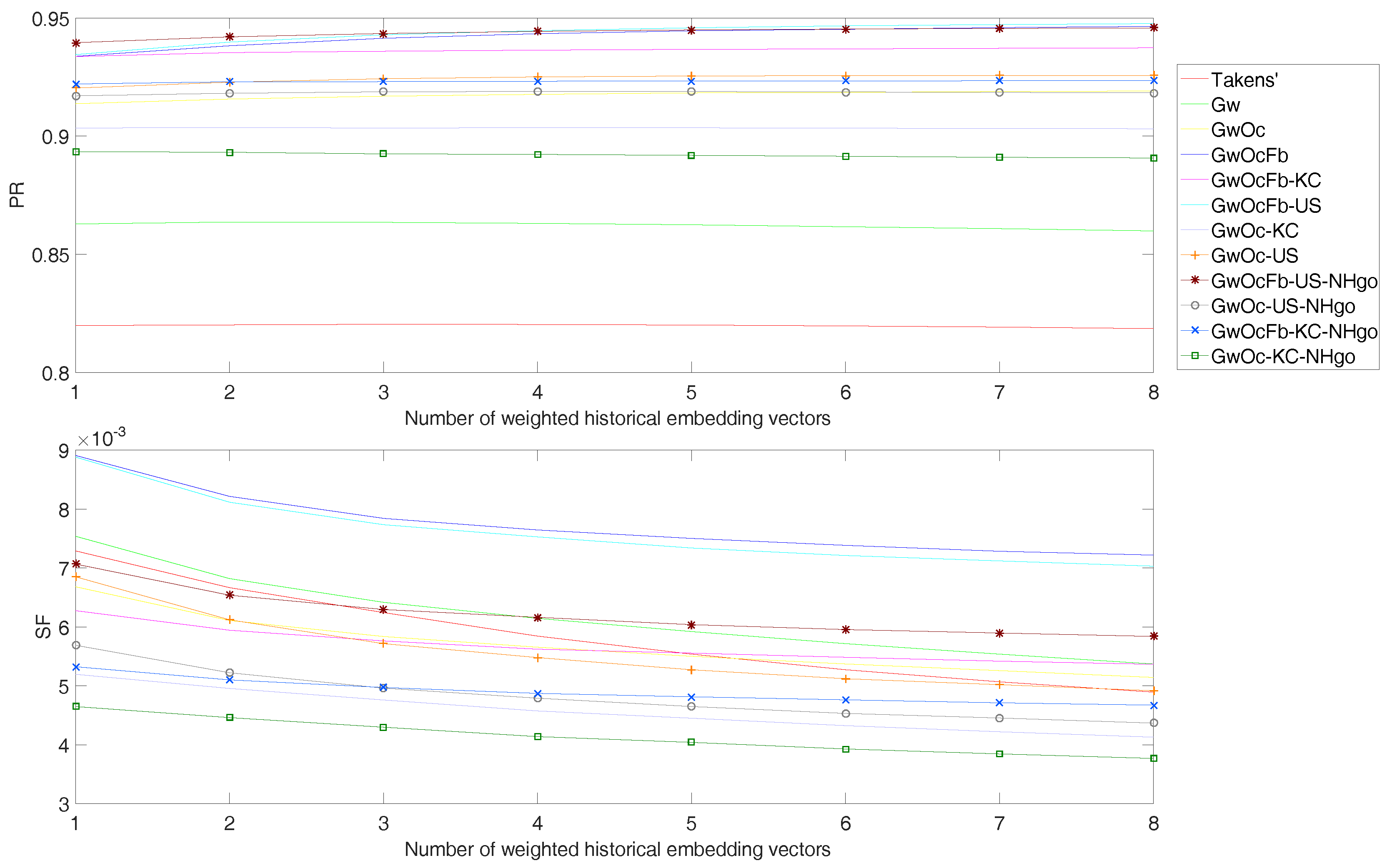
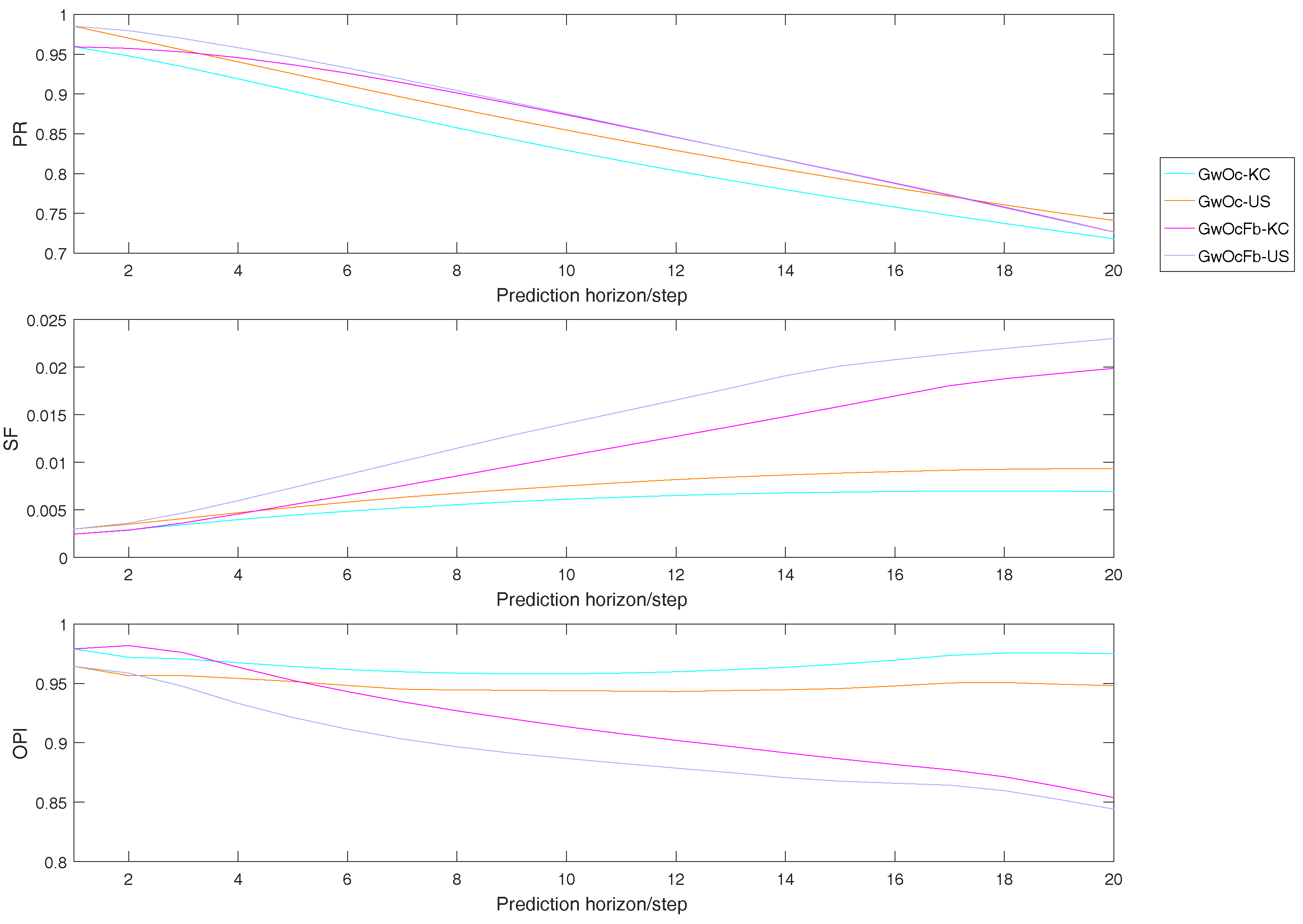
• It can seen more clearly in Figure 11 that when compared with the original Takens’ reconstruction method, the $PR$ and $SF$ values of Gw and GwOC had significant improvements, especially during the lower prediction horizon range, which meant the Gaussian weighting and offset correction were effective and the assumption of smoothness and consistency of human motion was reasonable.
• Also, it can be inferred by comparing GwOc, GwOc-KC, and GwOc-US that for prediction accuracy the synergy improvement of united source of history embedding vector generation had a positive effect on smoothness improvement and a negative effect on accuracy. In contrast, the improvement of Kalman fusion with complementary joint prediction played an opposite role. Hence, the two synergy improvements would be chosen based on application preference.
• Figure 11, Figure 12 and Figure 13 show that feedback scheme would push up the $PR$ value and hold back the $FS$ value. The $FS$ curves of the methods with feedback scheme deviated a lot from the other methods with the extension of the prediction horizon. This was always true by comparative inspection. Hence, if prediction accuracy is expected with highest priority, the feedback scheme should be considered.
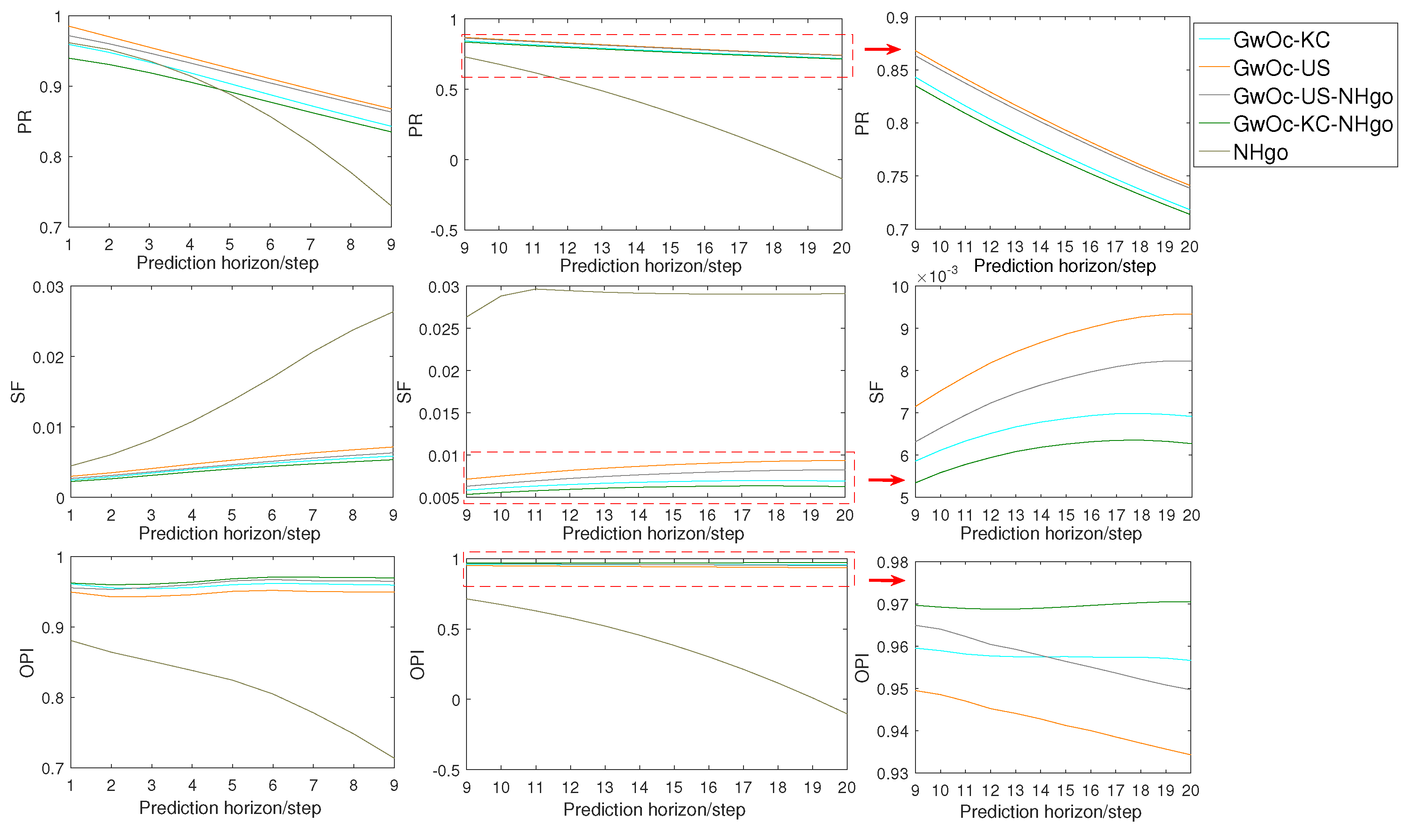
• In Figure 14, initially in the prediction horizon range of 1–3, the Newton’s method with a high-gain observer had a medium accuracy and also adequate smoothness, but after 3, the Newton’s method-based predictions degraded the fastest in both accuracy and smoothness. Meanwhile, for Takens’ reconstruction-based methods, the curves changed moderately. The NHgo-fused methods, GwOC-US-NHgo and GwOC-US-NHgo, exhibited a slight drop in $PR$ values compared to the methods without fusion, but the smoothness was more elevated. As a result, their overall performance was increased.
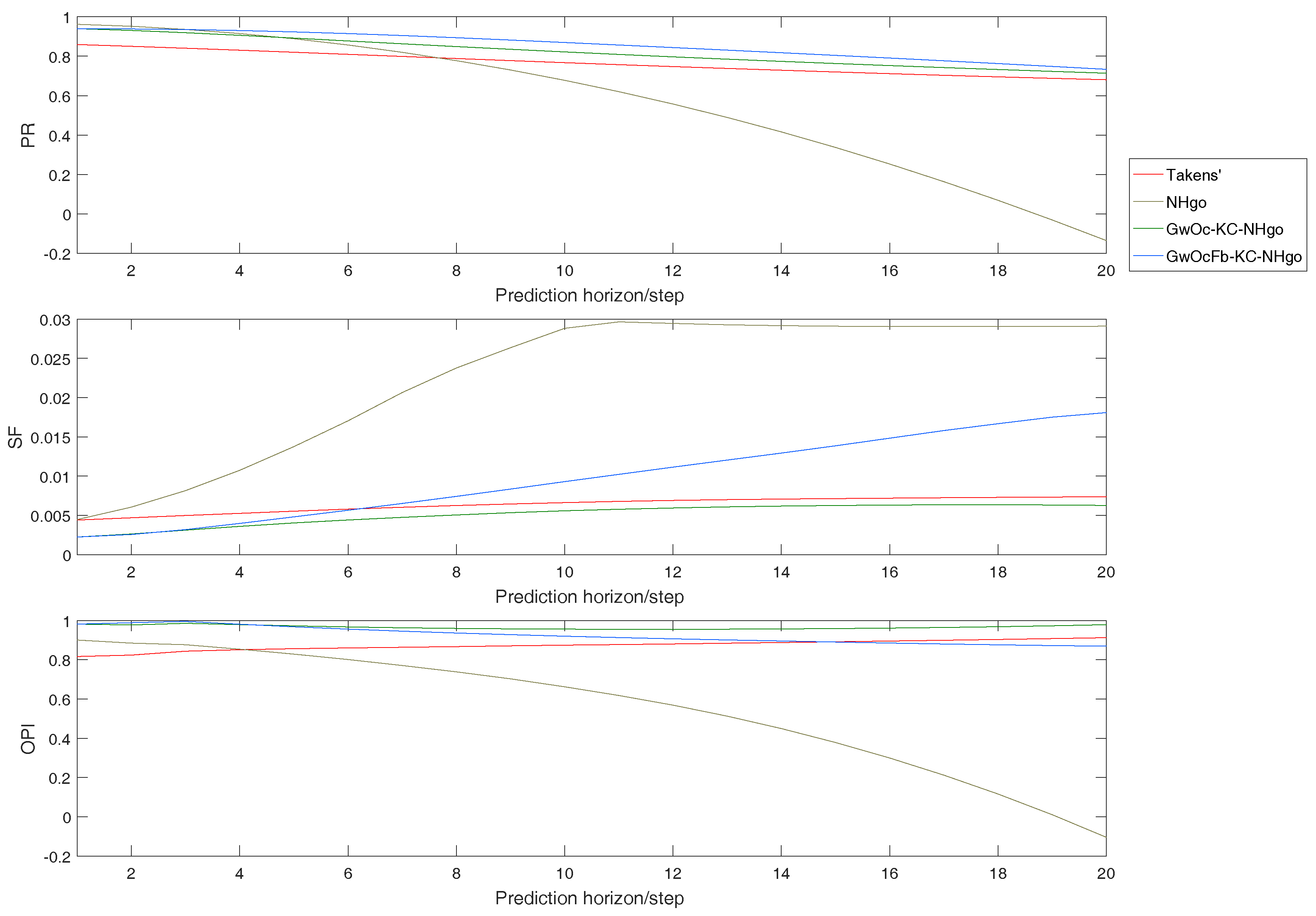
• By observing Figure 15 for short-term prediction such as in steps 1–3, the basic Takens’ reconstruction method’s performance was unsatisfactory, but its $OPI$ value rose gradually, which meant its relative performance over other methods increased. The $OPI$ curve with the KC-NHgo method changed gradually from an descending trend to ascending, which meant it was superior to other methods with respect to an extended prediction horizon. Considering the $OPI$ values with designed weighting, the fully improved method, GwOc-KC-NHgo, was apparently better across the prediction horizon range. The $OPI$ values are relative criterion and are significantly affected by the weighting value. If smoothness is preferred, the GwOc-KC-NHgo method is superior.

The adaptability to irregularities could be assessed visually and quantitatively by local irregularity tracking performance observations. The segments considered as irregularities in the assessment dataset were isolated and the predictions with different methods based on the parameters in Table 2 were executed. Some typical local trajectories are shown in Figure 16.

It can be seen in Figure 16a that a flat curve with zero values from 0 to 0.4 s exists at the very beginning of the predicted curves of Takens’ reconstruction methods. Noting that there are no human data (zero), this meant dead time existed. Zero dead time was gained by other methods via offset correction, feedback, and fusion with the Newton-based methods.

Figure 16b presents the performance of different methods during transitions. Except for the basic Takens’ reconstruction method, other methods were able to provide more or less prediction. The NHgo method-predicted curve fluctuated severely. Although the methods fusing the NHgo method, GwOc-KC-NHgo and GwOcFb-KC-NHgo, were influenced by these fluctuations locally, the fusion provided a better inhibiting effect. As the NHgo method exhibited outstanding prediction capability during periodicity loss, the methods fused with it acquired better prediction ability than without it.

Figure 16c,d were segments where periodicity was invisible, thus it was quite obvious that Takens’ reconstruction method could hardly provide prediction, while other methods still worked more or less.

Quantitatively, the numerical criteria could gave a more objective judgement. Figure 17 compared the $PR$, $OPI$, and $SF$ values between the whole dataset and the dataset during irregularities only. There are three phenomena worth noting in the figure:

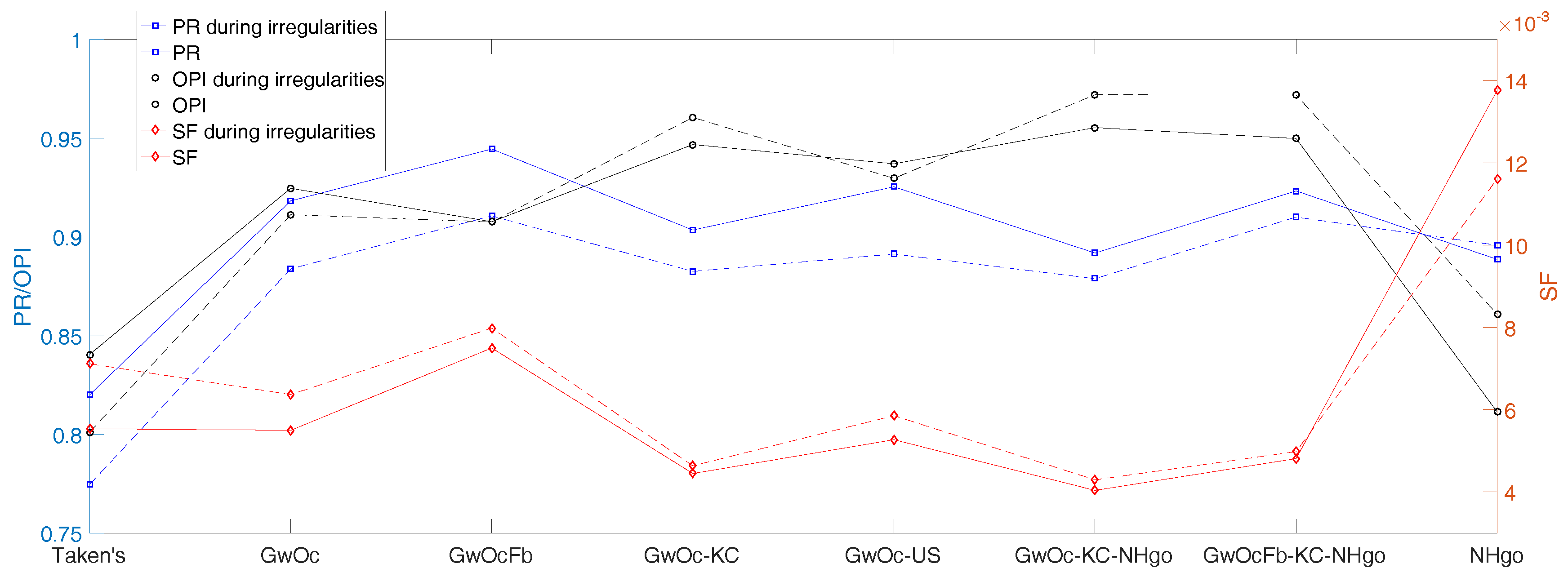
• The closing up of the assessment measure value gaps between the whole dataset and dataset during irregularities
• The improvement in the values’ changing trends.
• The signs of differences in assessment measure values between the whole dataset and dataset during irregularities.

Compared with the basic Takens’ method, the GwOc method closed up the gaps of $PR$, $SF$, and $OPI$ values between the whole dataset and the dataset during irregularities. Also, all the values were improved with a positive trend. Compared with the GwOc method, the GwOcFb method also made the gap even smaller, but the $SF$ values rose, which brought down the $OPI$ values. With a similar analysis, the GwOc-KC and GwOc-US methods elevated the smoothness with prediction accuracy degradation, and also narrowed the gaps, which means the synergy improvement was effective in improving the prediction performance.

The $PR$ value difference using the NHgo method with respect to the whole dataset and the dataset of irregularities is negative, which means the prediction accuracy adapted better to irregularities, while for the $SF$ values the difference is positive, which means the smoothness of predicted trajectories also adapted to irregularities better than periodicity. In contrast, the Takens’, GwOc, GwOc-KC, and GwOc-US methods adapted to the whole dataset better.

Thus, by fusing the two types of prediction methods, the GwOcFb-KC-NHgo and GwOc-KC-NHgo methods achieved acceptable accuracy and smoothness, and their adaptability to irregularities was improved. The OPI values for irregularities also demonstrated better adaptability of GwOcFb-KC-NHgo and GwOc-KC-NHgo over other methods, performing extremely well with the whole dataset and the irregular segments.

Based on the previous analysis, the GwOc-KC-NHgo method was the first choice for prediction because of its high prediction accuracy, smoothness, and adaptability to irregularities with no dead time.

4.3. Real-Time Demonstration

The GwOc-KC-NHgo methods were implemented on the human lower limb motion capture system in Figure 1 with the basic parameters designed as in Table 2. The algorithm’s computational time was between 3.2 and 3.3 ms (Figure 18) with tiny fluctuations which could satisfy the real-time execution requirements. The computational expenses of the other methods were similar, but could not be shown here.

5. Conclusions

In exoskeletal robot control, it would be much easier to handle the human robot coordination problem if the human motion was known in advance. Prediction is a helpful approach. Based on the biological features of human walking, a series of bio-inspired prediction methods were proposed and implemented. The parameters of Takens’ reconstruction-based methods were analysed and selected with the parameter robustness of newly introduced methods demonstrated as well. The comparative assessment demonstrated the offset correction and that Gaussian weighting techniques could effectively improve the prediction performance of Takens’ reconstruction method in both prediction accuracy and trajectory smoothness. The feedback scheme was useful in prediction accuracy improvement but degraded the smoothness. The synergy improvement of the coupled joints’ united source of historical embedding generation exhibited better performance in prediction accuracy than Kalman fusion with the complementary joint prediction and poorer performance in trajectory smoothness. The second-order Newton’s method with a high-gain observer gave acceptable performance with short prediction horizons. When considering improving the adaptability to irregularities, the Takens’ reconstruction-based methods were fused with Newton-based methods. On comparison with their contending methods, the new hybrid methods showed mixed features with nearly zero dead time, a slight deterioration in prediction accuracy and smoothness in short prediction horizons, and improvement in longer prediction horizons. The methods should be tailored for the detailed requirements of exoskeletal robot applications. When accuracy is emphasized, the GwOc-KC-NHgo method is recommended. The real-time computational expense would not be a burden for the methods introduced.

References

1. Sheridan, T.B. Telerobotics. Automatica 1989, 25, 487–507. [Google Scholar] [CrossRef]
2. Huang, L. Robotics Locomotion Control. Ph.D. Thesis, University of California, Berkeley, CA, USA, 2005. [Google Scholar]
3. Novak, D.; Reberšek, P.; De Rossi, S.M.M.; Donati, M.; Podobnik, J.; Beravs, T.; Lenzi, T.; Vitiello, N.; Carrozza, M.C.; Munih, M. Automated detection of gait initiation and termination using wearable sensors. Med. Eng. Phys. 2013, 35, 1713–1720. [Google Scholar] [CrossRef] [PubMed]
4. Kanjanapas, K.; Wang, Y.; Zhang, W.; Whittingham, L.; Tomizuka, M. A Human Motion Capture System Based on Inertial Sensing and a Complementary Filter. In Proceedings of the ASME 2013 Dynamic Systems and Control Conference on American Society of Mechanical Engineers, Palo Alto, CA, USA, 21–23 October 2013; p. V003T40A004. [Google Scholar]
5. Wang, M.; Wu, X.; Liu, D.; Wang, C.; Zhang, T.; Wang, P. A human motion prediction algorithm for non-binding lower extremity exoskeleton. In Proceedings of the 2015 IEEE International Conference on Information and Automation, IEEE, Lijiang, China, 8–10 August 2015; pp. 369–374. [Google Scholar]
6. Zhang, W.; Tomizuka, M.; Byl, N. A wireless human motion monitoring system for smart rehabilitation. J. Dyn. Syst. Meas. Control 2016, 138, 111004. [Google Scholar] [CrossRef]
7. Lin, Y.; Min, H.; Wei, H. Inertial measurement unit-based iterative pose compensation algorithm for low-cost modular manipulator. Adv. Mech. Eng. 2016, 8. [Google Scholar] [CrossRef]
8. Novak, D.; Riener, R. A survey of sensor fusion methods in wearable robotics. Robot. Auton. Syst. 2015, 73, 155–170. [Google Scholar] [CrossRef]
9. Fleischer, C.; Hommel, G. A Human–Exoskeleton Interface Utilizing Electromyography. IEEE Trans. Robot. 2008, 24, 872–882. [Google Scholar] [CrossRef]
10. Li, Z.; He, W.; Yang, C.; Qiu, S.; Zhang, L.; Su, C.Y. Teleoperation control of an exoskeleton robot using brain machine interface and visual compressive sensing. In Proceedings of the 2016 12th World Congress on Intelligent Control and Automation (WCICA), Guilin, China, 12–15 June 2016; pp. 1550–1555. [Google Scholar]
11. Iqbal, S.; Zang, X.; Zhu, Y.; Saad, H.M.A.A.; Zhao, J. Nonlinear time-series analysis of different human walking gaits. In Proceedings of the 2015 IEEE International Conference on Electro/Information Technology (EIT), Dekalb, IL, USA, 21–23 May 2015; pp. 25–30. [Google Scholar]
12. Pitkin, M.R. Effects of Design Variants in Lower-Limb Prostheses on Gait Synergy. JPO J. Prosthet. Orthot. 1997, 9, 113–122. [Google Scholar] [CrossRef] [PubMed]
13. Senda, S.; Takata, N.; Tsujita, K. A study on lower limb’s joint synergy in human locomotion with physical constraints on the knee. In Proceedings of the 2012 IEEE/SICE International Symposium on System Integration (SII), Fukuoka, Japan, 16–18 December 2012; pp. 349–354. [Google Scholar]
14. Sanzmerodio, D.; Cestari, M.; Arevalo, J.C.; Garcia, E. Exploiting joint synergy for actuation in a lower-limb active orthosis. Ind. Robot. Int. J. 2013, 40, 224–228. [Google Scholar] [CrossRef]
15. Rosenblatt, N.J.; Latash, M.L.; Hurt, C.P.; Grabiner, M.D. Challenging gait leads to stronger lower-limb kinematic synergies: The effects of walking within a more narrow pathway. Neurosci. Lett. 2015, 600, 110–114. [Google Scholar] [CrossRef] [PubMed]
16. Grimes, D.L.; Flowers, W.C.; Donath, M. Feasibility of an Active Control Scheme for Above Knee Prostheses. J. Biomech. Eng. 1977, 99, 215–221. [Google Scholar] [CrossRef]
17. Vallery, H.; van Asseldonk, E.H.; Buss, M.; van der Kooij, H. Reference trajectory generation for rehabilitation robots: complementary limb motion estimation. IEEE Trans. Neural Syst. Rehabil. Eng. 2009, 17, 23–30. [Google Scholar] [CrossRef] [PubMed] [Green Version]
18. Broer, H.; Takens, F. Reconstruction and time series analysis. In Dynamical Systems and Chaos; Springer: New York, NY, USA, 2011; pp. 205–242. [Google Scholar]
19. Herrmann, C. Robotic Motion Compensation for Applications in Radiation Oncology. Ph.D. Thesis, University of Würzburg, Würzburg, Germany, 2013. [Google Scholar]
20. Zhang, W.; Tomizuka, M.; Bae, J. Time series prediction of knee joint movement and its application to a network-based rehabilitation system. In Proceedings of the IEEE 2014 American Control Conference, Portland, OR, USA, 4–6 June 2014; pp. 4810–4815. [Google Scholar]
21. Zhang, W.; Chen, X.; Bae, J.; Tomizuka, M. Real-time kinematic modeling and prediction of human joint motion in a networked rehabilitation system. In Proceedings of the 2015 American Control Conference (ACC), Chicago, IL, USA, 1–3 July 2015; pp. 5800–5805. [Google Scholar]
22. Crowninshield, R.; Pope, M.H.; Johnson, R.; Miller, R. The impedance of the human knee. J. Biomech. 1976, 9, 529–535. [Google Scholar] [CrossRef]
23. Yangming, X.; Hollerbach, J.M. Identification of human joint mechanical properties from single trial data. IEEE Trans. Biomed. Eng. 1998, 45, 1051–1060. [Google Scholar] [CrossRef] [PubMed]
24. Zhang, L.Q.; Nuber, G.; Butler, J.; Bowen, M.; Rymer, W.Z. In vivo human knee joint dynamic properties as functions of muscle contraction and joint position. J. Biomech. 1997, 31, 71–76. [Google Scholar] [CrossRef]
25. Andrea, T.; Marcello, M. A low-noise estimator of angular speed and acceleration from shaft encoder measurements. J. Autom. 2001, 42, 169–176. [Google Scholar]
26. Ahrens, J.H.; Khalil, H.K. High-gain observers in the presence of measurement noise: A switched-gain approach. Automatica 2009, 45, 936–943. [Google Scholar] [CrossRef]
27. Nicosia, S.; Tornambe, A. High-gain observers in the state and parameter estimation of robots having elastic joints. Syst. Control Lett. 1989, 13, 331–337. [Google Scholar] [CrossRef]
28. Madgwick, S.O.H.; Harrison, A.J.L.; Vaidyanathan, R. Estimation of IMU and MARG orientation using a gradient descent algorithm. In Proceedings of the 2011 IEEE International Conference on Rehabilitation Robotics, Zurich, Switzerland, 29 June–1 July 2011; pp. 1–7. [Google Scholar]
Figure 1. The inertial measurement unit (IMU)-based lower limb motion capture system. (a) One IMU module. (b) The system worn on a testing subject and the illustration of joint angles in the human sagittal plane collected in this research.
Applsci 07 01130 g001
Figure 2. Takens’ basic reconstruction method workflow.
Applsci 07 01130 g002
Figure 3. The feedback scheme integrated into Takens’ reconstruction-based methods.
Applsci 07 01130 g003
Figure 4. Synergy improvement method (1) of Takens’ reconstruction-based methods.
Applsci 07 01130 g004
Figure 5. Synergy improvement method (2) of Takens’ reconstruction-based methods.
Applsci 07 01130 g005
Figure 6. The relationship map of different methods and improving approaches.
Applsci 07 01130 g006
Figure 7. Dataset for prediction method assessment (the joint angles of the knees and hips of a test subject in a sagittal plane collected by the inertial measurement unit-based motion capture system).
Applsci 07 01130 g007
Figure 8. Influence of history data length used in embedding vector generation (left hip joint data in the sagittal plane). S F : smoothness factor; P R : prediction ratio.
Applsci 07 01130 g008
Figure 9. Influence of embedding vector length (left hip joint data in the sagittal plane).
Applsci 07 01130 g009
Figure 10. Influence of weighted historical embedding vector number (left hip joint data in the sagittal plane).
Applsci 07 01130 g010
Figure 11. Comparison of prediction performance between the Takens’, Gw, GwOc, GwOcFb, GwOc-KC, and GwOc-US methods (left hip joint data in the sagittal plane). O P I : overall performance index.
Applsci 07 01130 g011
Figure 12. Comparison of the prediction performance of the GwOc-KC, GwOc-US, GwOcFb-KC, and GwOcFb-US methods (left hip joint data in sagittal plane).
Applsci 07 01130 g012
Figure 13. Comparison of the prediction performance of the GwOc-KC-NHgo, GwOc-US-NHgo, GwOcFb-KC-NHgo, GwOcFb-US-NHgo methods (left hip joint data in the sagittal plane).
Applsci 07 01130 g013
Figure 14. Comparison of the prediction performance of the GwOc-KC, GwOc-US, GwOc-KC-NHgo, GwOc-US-NHgo, and NHgo methods (left hip joint data in the sagittal plane).
Applsci 07 01130 g014
Figure 15. The comparison between Takens’, NHgo, GwOc-KC-NHgo and GwOcFb-KC-NHgo methods (left hip joint data in the sagittal plane).
Applsci 07 01130 g015
Figure 16. Typical adaptability of different methods to irregularities (left hip joint angle in sagittal plane). (a) Dead time during initiation; (b) Speed transition from 1 km/h to 2 km/h; (c) Stand–walk transition; (d) Non-periodic motion during “stopping and leaving the treadmill”.
Applsci 07 01130 g016
Figure 17. Performance of different methods during irregularities (left hip data).
Applsci 07 01130 g017
Figure 18. Real-time computational expense of the GwOc-KC-NHgo method (left hip data at 2 km/h walking).
Applsci 07 01130 g018