1. Introduction
Offshore wind farms using fixed substructures are mostly constructed in seawaters having a depth of less than 40 m, and this often limits the number of wind turbines that can be installed in a wind farm. The spacing between wind turbines commonly range from 7 RD to 11 RD, where RD represents the rotor diameter of the wind turbine [
1,
2]. Considering the fact that the rotor diameters of modern wind turbines commonly reach 100 m, the spacing between wind turbines seems large but it is still necessary to reduce the wake effects from upstream wind turbines on downstream ones which result in lower power and higher load [
3].
Investigations on active induction wind farm control to reduce the wake strength by regulating the power of the upstream wind turbines less than their available power have been done by researchers. Earlier research articles were focused on the phenomenon itself, and the physical explanations of the power increase using one-dimensional momentum theory were presented [
4,
5]. The simple model predicted an increase of 4.1% of the total power of two turbines in line when the induction of the first wind turbine was reduced from 1/3 to 1/5. In addition, to prove the idea, wind tunnel tests with micro scale wind turbine model arrays with manually adjustable blade pitches with a turbine spacing of 4.5 RD were used. From the scaled farm measurements, about 4.5% of increase in the total power was observed with a blade pitch angle of 2°. However, later, the measurement uncertainty turned out to be greater than the power increase 6%, and the results were also found to be greatly affected by the Reynolds number effects occurring only in wind tunnel tests [
5,
6]. In addition, a few field measurements with multi-MW wind turbines with a 3.8 RD spacing were tried but not very successful [
5,
6] to make a quantitative conclusion. Later, the field data were reanalyzed for two 2.5 MW wind turbines with a spacing of 3.8 RD, and turned out to have a power increase of about 5% with a fixed pitch angle of 2° [
7].
After that, the active induction wake control method based on the manual blade pitch adjustment (change of axial induction) was applied to a simple wind turbine model with an engineering wake model. The simulation concluded that the adjustment of the blade pitch angle can increase the total power of a wind farm by about 10% [
8,
9,
10].
Later, articles focused on various wind farm control algorithms including genetic algorithms were presented [
11,
12,
13,
14]. Some were wind farm model based methods and some were model free methods. Because it is very hard to prove the wind farm control effects on the farm power output in real wind farms, all validations were made with simulations. In addition, the facts that a wind farm simulation must deal with multiple wind turbines, and simulations with multiple wind turbines require large computational loads, limited the simulations to be the simulations of simple wind turbine models without any dynamics in conjunction with a simple wake model. The wind turbine models were simply algebraic equations with power coefficient and the simulations were made with constant wind speeds and no turbulence. The power gains from these simplified static analyses varied from 0.6% to 25% depending on the control method [
11,
12,
13,
14]. In addition, some researchers tried to change the wind turbine operating point to reduce the wake effect based on simple wind turbine models with engineering wake models and they concluded with power increases of 1.86% to 6.24% [
8]. However, the results are considered to be exaggerated due to the simple wind turbine model and the constant wind.
Recently, an extremum seeking control as a model-free method was used to prove the algorithm. The simulation was done in turbulent winds with a few different turbulence intensities [
15] but the wind turbine model was still a simple algebraic equation that does not have any system dynamics. In the study, the controller was successful with low turbulence intensity. However, the controller failed with high turbulence intensity which was about 0.21. This was because, with high turbulence intensity, the controller could not distinguish power variations due to wind speed change from those due to wind farm control.
More recently, the concept of power increase by regulating the power of the most upstream wind turbine was reinvestigated with a relatively high fidelity wind farm simulation model [
16]. In the research, it was found that the power partialization percentage, defined as the power output to the available power of the most upstream wind turbine to achieve the maximum power of a wind farm, is a function of the wind turbine spacing but is not much affected by the wind speed. Therefore, the power regulation of the upstream wind turbine for power maximization is achieved not by a constant blade pitch angle but by a constant power partialization of the most upstream wind turbine. This means that the blade pitch angle of the most upstream wind turbine must be adjusted when the wind speed varies. In the study, a power increase of 4.1% was observed with ten wind turbines in series with a spacing of 4 RD when the partialization of the most upstream wind turbine was 0.825. However, in that study, the wind was not a turbulent wind but a constant wind, and the study did not include any wind farm control algorithm, but did include results with manual power adjustments of the most upstream wind turbine for better understanding of power increase mechanism.
There have also been conflicting results in the literature that the active induction of the most upstream wind turbine does not increase the overall power output from the wind farm [
17,
18]. They are mostly based on the simulation results with the LES (Large Eddy Simulation) method. Nilsson et al. [
17] applied the LES to simulate the Lillgrund wind farm and showed the simulation results with the ambient turbulence intensity of 5.6% that the manual blade pitching of the first wind turbine by multiples of 2° does not increase the total power. However, in their study, the wind turbine dynamic and control was not considered. In addition, Annoni et al. [
18] applied the high fidelity simulation tool, SOWFA (Simulation fOr Wind Farm Applications) to investigate the power increase of a small wind farm of five wind turbines by power curtailment. However, the manual blade pitching of the most upstream wind turbine did not increase the total farm power, but rather decreased it approximately by 8.9%. In their simulation results with five wind turbines in series, the powers of all four wind turbines except the fifth one decreased with the power curtailment of the most upstream wind turbine. They concluded that for the total power increase, a suitable wind farm control is necessary. Goit and Meyers [
19] applied an optimal control strategy to the LES simulation with an actuator disk model to investigate the total power increase of a wind farm with 50 wind turbines. Unlike other LES simulations with the fixed blade pitching, they found the power increase of 16% compared with the uncontrolled case. However, the wind turbine dynamics and power control algorithms of wind turbines including blade pitch (most upstream wind turbine only) and generator torque (all wind turbines) controls were not considered in their study.
In this study, the previous study [
16] was further expanded to develop a model based wind farm control method with a simple but effective open-loop wind farm control algorithm based on a function minimization method. The command from the wind farm controller to the wind turbine was the active power of the wind turbine and the wind farm control algorithm was validated with the relatively high fidelity wind farm model constructed previously [
20] but modified for this study. The originality of this study compared with the previous research can be summarized by the following factors.
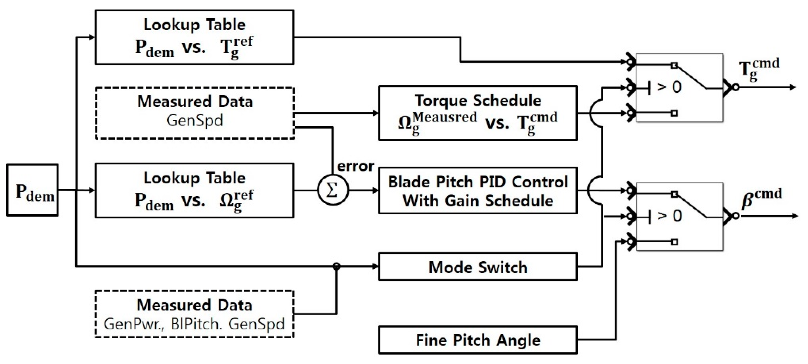
First, the proposed wind farm control in this study considered implementation of the control in actual wind farm controllers that receive data from wind turbines and give commands to them without affecting the built-in wind turbine torque and pitch control algorithm for maximum power point tracking and power regulation. By considering the fact that modern multi-megawatt wind turbine controllers use the torque and rotating speed of the generator as targets to achieve power maximization or regulation, the variable of the most upstream wind turbine used for a wind farm control was chosen not to be the blade pitch angles or axial induction factors that used for the previous articles [
3,
4,
5,
6,
7,
8,
9,
10,
11,
12,
13,
14,
15] but to be the generator power. The generator power can be expressed as the torque multiplied by the rotating speed of the generator, and, therefore, the power regulation of the most upstream wind turbine could be done without affecting its built-in control algorithm. However, the wind turbine controller of the wind turbine model in the wind farm simulation tool had to be modified to additionally include a demanded power tracking control algorithm.
Second, by considering the fact that the optimal power partialization of the most upstream wind turbine is not much affected by the wind speed [
16], a simple open loop control with power command output to wind turbines was implemented to the wind farm controller. Modern multi-megawatt wind turbines already use open-loop control for maximum power point tracking when the wind speed is lower than the rated wind speed [
21,
22,
23]. In addition, a simple open-loop dispatch wind farm control based on the available powers of the wind turbines in a wind farm is already implemented for a power demand tracking in wind farms. Therefore, a simple but effective open-loop wind farm control for a total power increase in a farm was not new in this area and was chosen for this study. The proposed wind farm controller consists of a wind speed estimator, optimal power command calculator and a wind farm model. It calculates the available power at a chosen control frequency, finds the optimal power commands to individual wind turbines based on its wind farm model, and sends the commands to wind turbines for power increase and load reduction.
Thirdly, the proposed wind farm control algorithm was validated not with a simple model without any dynamics under steady wind but with a high fidelity wind farm simulation tool under turbulent wind with wind turbine dynamics and controls. For this, the wind turbine controller for power command tracking as well as the wind farm controller were constructed and implemented to the high fidelity simulation tool [
16]. Therefore, more realistic simulation results can be obtained compared to the previous studies [
4,
5,
6,
7,
8,
9,
10,
11,
12,
13,
14,
15,
16,
17,
18,
19] for the validation of the proposed wind farm control algorithm.
4. Discussion
To fully understand the proposed wind farm control, parametric studies for turbine spacing, turbulent intensity and control frequency were made.
4.1. Total Power
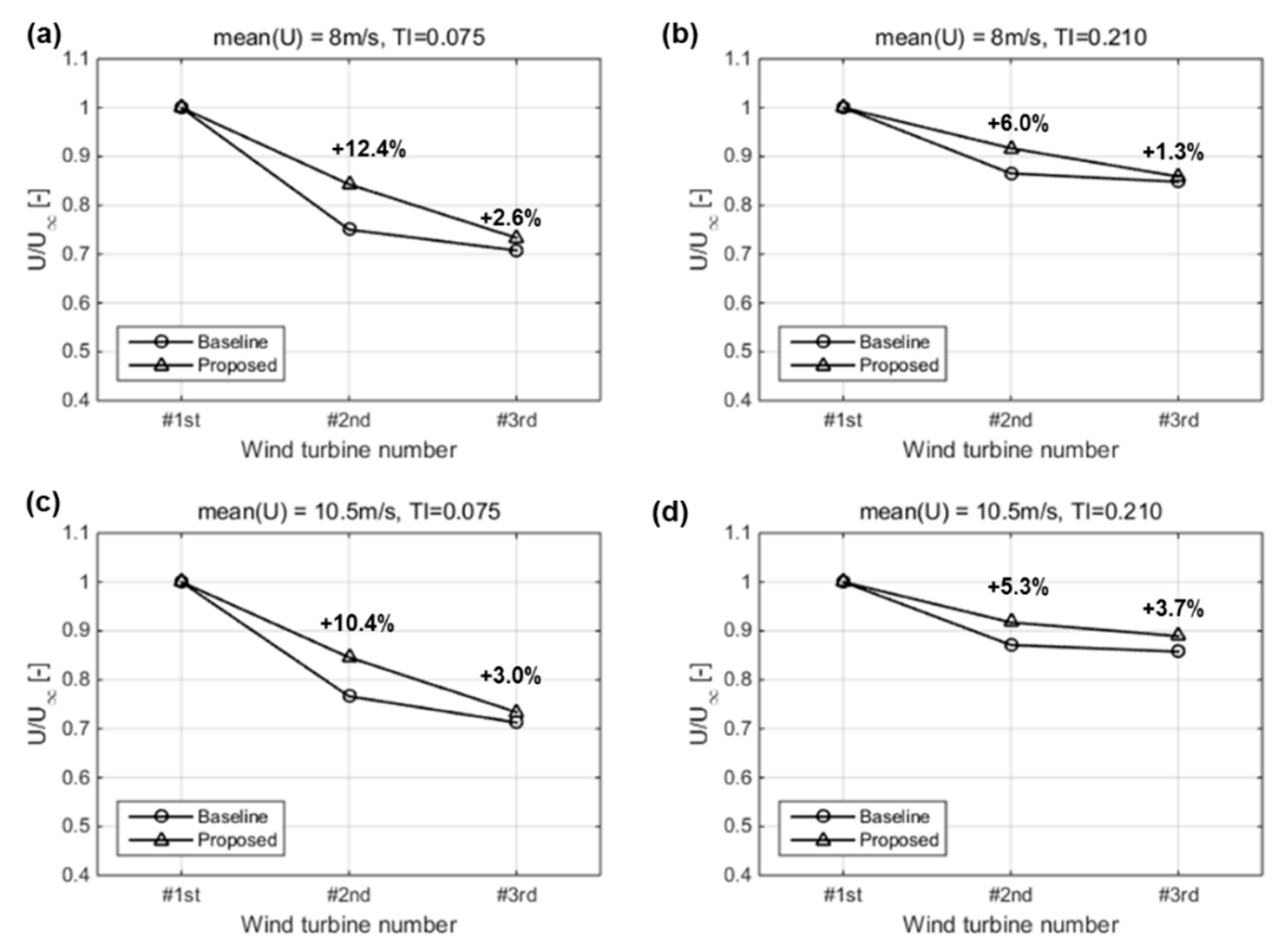
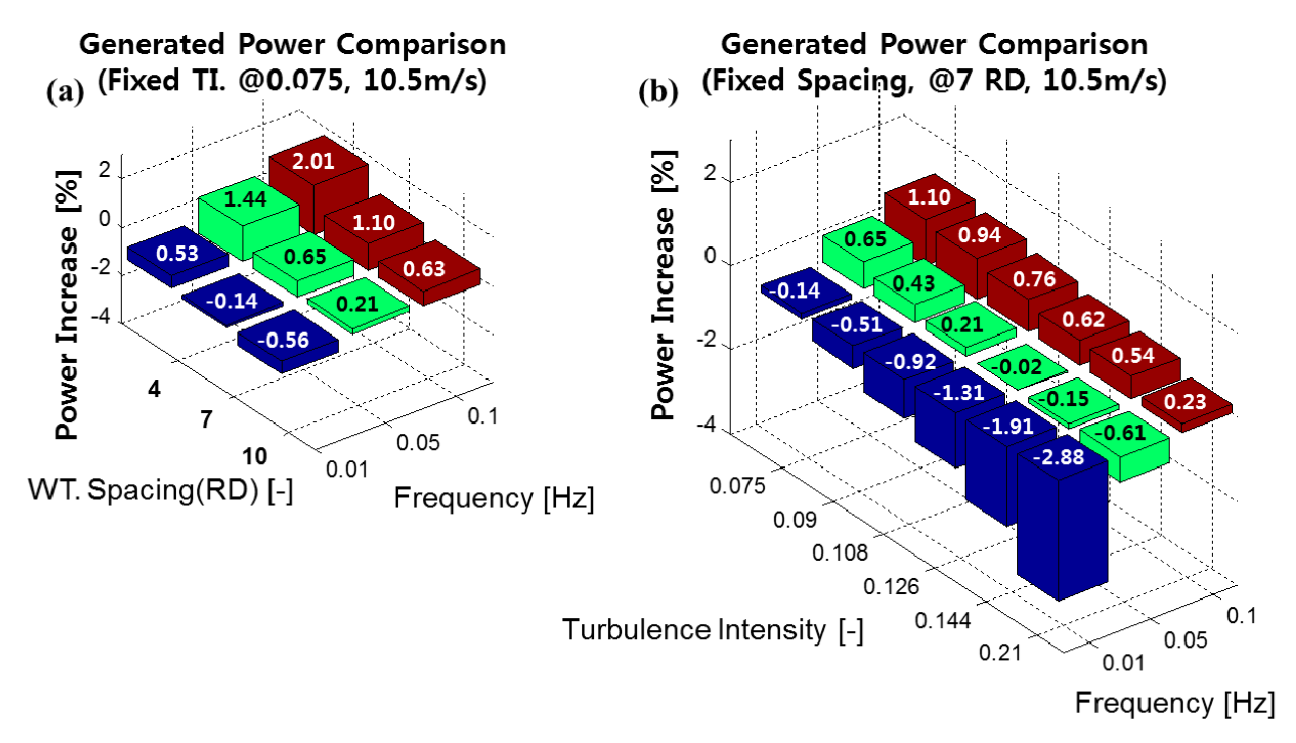
Figure 10 and
Figure 11 show the power increase of the proposed wind farm control in percentage relative to the power of the baseline control for two different mean wind speeds, 8 m/s, and 10.5 m/s.
Figure 10a,b presents 8 m/s, and
Figure 11a,b presents 10.5 m/s. Two wind speeds were chosen for simulation because they correspond to two different wind turbine control regions. The former is the control region for maximum power coefficient and the latter is the control region for smooth transition from the maximum power coefficient control and the rated power control. Based on the figure, it can be found that the power increase of the proposed controller with respect to the power with the baseline controller decreases with increasing wind turbine spacing and increases with increasing control frequency. In addition, the power increase decreased when the ambient turbulent intensity increased. This is partly because more fluctuations in wind speed make the power commands to the wind turbines deviate more from the optimal values. In addition, this is because, with the higher turbulence intensity, the wake recovers more rapidly, and, therefore, the wake loss with the baseline controller is reduced and finally the effect of active induction control is reduced. The power increase was reduced when the wind speed is in the transition control region. When the turbine spacing reached 10 RD, no power increase was observed. It is because when the turbine spacing is 10 RD, the wake loss due to the upstream wind turbine is small. In addition, when the turbulence intensity was large such as 0.21, the power with the proposed control became even lower than the power with the baseline controller when the control frequency was 0.01 or 0.05. This is because the wind farm controller runs too slow to effectively track the high wind speed variation.
However, when the control frequency was 0.1 Hz, although the ambient turbulence intensity was 0.21, the power with the proposed control became higher again than the power with the baseline control. When the turbine spacing was 7 RD the increase was 2.29%. In the previous study with an extremum seeking control [
15], a similar decreasing trend in the power gain relative to the baseline control was observed with increasing ambient turbulent intensity, but, with the ambient turbulence intensity of 0.21, the controller failed to distinguish the change in power by control from the change in power by turbulence, and the power gain became negative.
4.2. Tower Load
Figure 12 shows the variation of tower load with respect to the turbulence intensity and the control frequency. It is the result when the turbine spacing is 7 RD. As shown in the figure, for all the cases, the tower load of the most upstream wind turbine decreased dramatically.
Although the loads of the downstream wind turbines increased, they were kept lower than the load of the most upstream wind turbine. However, as the control frequency increased from 0.01 Hz to 0.1 Hz, the tower load increased. This is because the wind turbine uses more pitch action with higher control frequency. In addition, it can be found from the figure that the decrease in tower load of the most upstream wind turbine decreases with increasing ambient turbulent intensity. When the ambient turbulence intensity was 0.21, the decrease from the value of the baseline controller was 9.2%. The reason why the tower load increases with the ambient turbulent intensity is because more pitching action occurs in the blade of the wind turbine.
4.3. Comparison of Other Models
Table 2 shows the experimental and simulation results of wind farm control available in the literature for comparison. A few experimental results are available in the literature. Based on the table, the results from the experiment showed 4.5–5% increase in power with the manual blade pitching of 2°. However, more experimental validation seems necessary for a concrete conclusion. The simulation results using the Jensen linear wake model showed relatively high power increase. They were 10.57% increase with an optimal control and 6.24% increase with a manual adjustment of the tip speed ratio (TSR). The simulation results with more advanced wake models based on Parabolic Reynolds averaged Navier–Stokes equation (RANS) such as Ainslie’s eddy viscosity model or UPMWAKE showed the power increase from 2.85% to 4.5% depending on the turbine spacing and the control type. The power increases were slightly lower than those from the Jensen wake model because the Jensen model with the wake decay constant of 0.04 (recommend for offshore application) is known to be equivalent to the ambient turbulence intensity of approximately 8–10%. Therefore, the wake recovery with the Jensen model is expected to be faster than the wake recovery in the location where the turbulence intensity is lower than. The results from the LES simulation with an actuator disk or an actuator line method showed some discrepancy. The manual blade pitching with the LES simulation showed the power decreases of −2.2% and −8.9% with the blade pitching angle of 2°. The largest decrease in the power was obtained with five wind turbines in series and, with the blade pitching of the most upstream wind turbine, the power outputs from the four upstream wind turbine were all decreased and the power of the fifth wind turbine was slightly increased compared with the reference baseline control. The reason for this unusual result is explained to be due to the wake meandering effect by the authors of the literature. Unlike the two results with the LES simulation, the optimal control algorithm applied to the LES simulation with an actuator disk model showed the power increase of 16%. However, the wind turbine control algorithms and wind turbine dynamics were not used in the study and this might reduce the power increase. Although the results in
Table 2 were obtained with different conditions and cannot be compared directly, the results in this study with the proposed model predictive open loop wind farm control are within the range of the results obtained from other studies, and the power gains are relatively low. The reason for this is considered to be that more realistic conditions including wind turbine dynamics, wind turbine control, and wind farm control frequency have been added in the simulation of this study. However, experimental study must be done as a future work to fully validate the result.
4.4. Strengths and Weaknesses of the Current Study
The strengths of the current study can be summarized as the following two points. First, the current study considered the actual application of the wind farm control algorithm to the real wind farm, and proposed a simple but effective open loop wind farm control which can be fully applied to a wind farm controller (hardware) and used without affecting the current wind turbine control algorithms. The wind farm controller receives the measured generator speed, blade pitch angle, and the power output from the wind turbine controller and sends the optimal power command to the wind turbine controller.
In addition, the proposed wind farm control algorithm is validated in a relatively high-fidelity wind farm simulation tool [
20], which has wind turbine dynamics and control including the basic torque and pitch controller slightly modified to include the demanded power point tracking (DPPT) control [
37]. Therefore, the current wind farm simulation is almost the same as the real wind farm in terms of control. In addition, the wind farm control frequency applied was at least 10 times slower than the wind variation in the simulation to get more realistic simulation results. Parametric studies including turbulence intensities, turbine spacing and wind farm control frequencies were made to see the effects of active induction control on the total power increase in some more detail.
This study also has some weaknesses and they are as follows. The wake model used in this study is Ainslie’s eddy viscosity model which uses the thin boundary layer approximation on the RANS (Reynolds Averaged Navier–Stokes) equation with the empirical boundary condition obtained from the wind tunnel test. Although the model or its modified version is commonly used in commercial software for calculating the power outputs of a single or multiple wind turbines including the wake effect, the accuracy of the model needs to be experimentally validated with various wind turbine operating conditions.
In addition, in this study, the wake meandering is not considered. If the meandering is considered, the power decrease in the wake region might be changed and, therefore, the performance of the proposed wind farm control algorithm will be affected. Therefore, in the future, experimental validation of the simulation results needs to be performed.
5. Conclusions
A simple but effective model based open-loop wind farm control algorithm was proposed and validated with a relatively high-fidelity simulation tool in this study. The wind farm model for control was a simplified version of the wind farm model for dynamic simulation, and consisted of a wind turbine model, wake model, wind propagation and superposition model, and a wind farm control model. Unlike the wind farm model for simulation, it had a look-up table based wind turbine model that does not have wind turbine dynamics. The wind farm model was used in the wind farm controller to find optimal power commands to individual wind turbines. With a function minimization algorithm, the wind farm control algorithm was validated with dynamic simulations with turbulent winds. For a virtual wind farm with three wind turbines in series, simulations were performed for both the baseline and the proposed wind farm controllers at the mean wind speed of 8 m/s. As the result, the proposed wind farm controller was found to increase the total power output by about 2.4% and to decrease the load of the most upstream wind turbine in DEL by about 16.7% when the turbulence intensity was 0.075 and the control frequency was 0.1 Hz.
In addition, parametric studies were performed to understand the power increase of the proposed wind farm controller compared with the baseline controller for different turbulent wind speeds different turbulence intensities and different control frequencies. The power increase was found to decrease as the turbine spacing increases and it decreased to about 1.5% when the turbine spacing was 10 RD at the mean wind speed of 8 m/s. In addition, the power increase was found to decrease as the turbulence intensity increases and it decreased to about 0.83% when the turbulence intensity was increased to 0.21. When the mean wind speed was close to the rated wind speed, the power increase was also found to decrease.
Although no wind direction change was considered in the current study, the effect of the model based wind farm control algorithm was found to be effective to increase power and reduce load in a wind farm. However, in the current study, the Ainslie’s eddy viscosity wake model was used to calculate the wind speed in the wake region, and Taylor’s frozen turbulence assumption was used for wind speed propagation. Therefore, the results need to be experimentally validated in a wind tunnel or in the field for better understanding.


