Article

A New Fuzzy Sliding Mode Controller with a Disturbance Estimator for Robust Vibration Control of a Semi-Active Vehicle Suspension System

1
Department of Mechanical System Engineering, Incheon National University, Incheon 22212, Korea
2
Department of Mechanical Engineering, Inha University, Incheon 22212, Korea
*
Author to whom correspondence should be addressed.
Appl. Sci. 2017, 7(10), 1053; https://doi.org/10.3390/app7101053
Submission received: 12 September 2017 / Revised: 18 September 2017 / Accepted: 11 October 2017 / Published: 13 October 2017

Abstract

:
This paper presents a new fuzzy sliding mode controller (FSMC) to improve control performances in the presence of uncertainties related to model errors and external disturbance (UAD). As a first step, an adaptive control law is designed using Lyapunov stability analysis. The control law can update control parameters of the FSMC with a disturbance estimator (DE) in which the closed-loop stability and finite-time convergence of tracking error are guaranteed. A solution for estimating the compensative quantity of the impact of UAD on a control system and a set of solutions are then presented in order to avoid the singular cases of the fuzzy-based function approximation, increase convergence ability, and reduce the calculating cost. Subsequently, the effectiveness of the proposed controller is verified through the investigation of vibration control performances of a semi-active vehicle suspension system featuring a magnetorheological damper (MRD). It is shown that the proposed controller can provide better control ability of vibration control with lower consumed power compared with two existing fuzzy sliding mode controllers.

Graphical Abstract

1. Introduction

In a practical environment, an enhancement of control performances in the presence of uncertainties related to model errors and external disturbance (UAD) is an important issue in various fields, as it affects vibration control in vehicle suspension systems, and the accurate tracking control of robotic systems. In order to develop more advanced control methods to deal with this issue, many approaches have been proposed for last two decades, including fuzzy logics (FL) [1,2,3,4,5,6], sliding mode techniques [1,7,8,9,10,11,12,13,14], a compensator design for UAD [15,16,17], and hybrid control methods [18,19,20,21,22,23]. Among those, the sliding mode control (SMC) is recognized as one of the best control techniques for control systems subjected to UAD. The typical advantages of SMC include implementation simplicity, robustness against uncertainties, and capability to deal with UAD. In addition, it is easy to coordinate with other mathematical tools [14,24]. To exploit SMC, firstly, a switching surface or sliding surface needs to be chosen based on the specific control aim. The system is then controlled to direct towards the sliding surface in the first phase (approaching phase); then, it upholds the switching surface in the second phase (sliding phase). If the dynamic process is stable, the state variables of the system are maintained on this switching surface [25,26] regardless of the inherent dynamics. The ability to reach the sliding surface and keep system states on this surface indicates the performance quality of the SMC. In various systems, this ability can be accomplished by integrating the SMC with the FL, named, a fuzzy sliding mode controller (FSMC) [27,28,29,30,31]. As is well known, the fuzzy system is a kind of approximated function with a high degree of flexibility. This inherent feature has meant that FL is used as a powerful tool in many control approaches [22,23,32].
Through using the combination of the SMC and FL, the salient advantages of each control strategy are kept during control action. For example, the fuzzy system is used to approximate unknown functions, while the sliding mode approach adds the possibility of establishing stable adaptation laws [32]. Therefore, as a type of robust controller with strong points, FSMC has been widely used in many application fields [27,28,29,30,31]. In addition, the design of a FSMC and estimator (or observer) for external disturbances can be independently carried out [15,33]. An adaptive fuzzy SMC for nonlinear active suspension vehicle systems that was subjected to uncertainty due to time-variation of the sprung mass was studied in [25], in which the Takagi–Sugeno (T–S) fuzzy model was utilized to handle the uncertainty. More practical systems whose control signals are based on the state variables have been used in several research works [1,12,18,23,31]. For example, Mohammad et al. showed an optimal adaptive fuzzy sliding mode controller for a class of nonlinear systems subjected to UAD [12], and the use of FL systems to approximate a plant’s unknown functions was proposed in [18,23,31]. Mojtaba et al. have shown that controlling the system over the network may introduce different constraints and conditions [32]. Some of these constraints and conditions may cause delays in control signal, data quantization, safety, and security.
One significant issue for designing a combined (or hybrid) controller using more than two different control techniques is the time varying rate of UAD. In the previous work by the authors of this current work, it was proven that when the time varying rate of UAD is increased, the quality of the controller is reduced [1,2]. Moreover, the control system could become unstable due to external disturbances. In order to resolve the problems caused from the high rate of time-varying parameters, in this work, a new FSMC system is formulated, and its effectiveness is shown through experimental implementation to a semi-active vehicle suspension system. Consequently, the technical novelty of this work is to propose a new FSMC associated with a disturbance estimator (DE) to enhance vibration control performance under severe operating conditions. Therefore, the main technical contributions of this work are summarized as follows.
(1) A new FSMC with a disturbance estimator DE (named DE-FSMC) that can adaptively identify plants via the online without complete knowledge about dynamic characteristics is formulated. The proposed controller has several features compared with the previous FSMC. One of the main difference is that the difficulty caused from the high rate time-varying parameters can be resolved by utilizing compensative parameters, while the previous FSMC can work for only the slow rate time-varying parameters. In addition, the calculating cost of the estimating parameters is less than that of the previous FSMC.
(2) In the design process, the UAD is separated into two groups related to uncertainties and external disturbances in order to deal with them individually. The first group is estimated by the fuzzy structure of the FSMC, while the second by the DE. Subsequently, an adaptive control law based on Lyapunov stability analysis is formulated to update the parameters of the DE-FSMC so that both the closed-loop stability and the finite-time convergence of the tracking error are guaranteed.
(3) In order to validate the effectiveness of the proposed control method, an experimental investigation is undertaken by adopting a semi-active vehicle suspension system installed with magnetorheological damper (MRD). Then, a comparative work between the proposed control method and two existing fuzzy sliding mode controllers is undertaken.

2. Problem Formulation

In order to design the proposed controller, the following equation is adopted.
{ x ( n ) = f ( x , t ) + g 1 ( x , t ) u ( t ) + g 2 ( t ) d ( t ) y = x
In the above, d ( t ) is the unknown time-dependent external disturbances. In Equation (2), f ( . ) and g 1 ( . ) become unknown nonlinear functions, which need to be identified. In this work, a new type of control law via estimating the d ^ ( t ) of d ( t ) and the f ^ ( . ) and g ^ 1 ( . ) of f ( . ) and g 1 ( . ) is built. By this way, the effectiveness of estimating UAD can be improved, since the time varying rate of d ( t ) is low. This approach has two combined phases, as shown in Figure 1. This figure represents a basic controller called a B-controller and a disturbance estimator DE. Thus, the control signal u ( t ) for the plant is to be totalized as follows: u ( t ) = u s ( t ) + d ^ ( t ) . In order to construct the total controller, the FL and SMC methods are to be used, in which the unknown functions f ( . ) , g 1 ( . ) in Equation (1) are approximated by the fuzzy structures. It is noted that although d ( t ) is ignored, the impact of model error on the system during the calculation process is compensated by the fuzzy structure of the B-controller. In order to investigate the DE for estimating d ^ ( t ) of d ( t ) , the known functions f 0 ( . ) and g 0 ( . ) are utilized.
The second issue relates to the function approximation. In order to establish f ^ ( . ) and g ^ 1 ( . ) , a sliding surface S ( x ) defined via the error e ( t ) between x ( t ) and x d ( t ) is formulated as follows [12,18]:
u s ( t ) = 1 g ^ 1 ( x , t ) ( f ^ ( x , t ) + x d ( n ) + F ( e ( t ) , S ) ρ G ( S , t ) )
where, F ( e ( t ) , S ) denotes the expression related to e ( t ) and S; G ( S , t ) is the function of S and t ; and ρ is the gain parameter. It can be observed from the equation that since g ^ 1 ( x , φ g ) is generated online, there is no guarantee such that g ^ 1 ( x , φ g ) 1 remains during the operating process. This method is liable to appear in singular cases in the calculating process. In order to avoid the singular cases, in this work, a solution via the role of ε 0 λ T ( x ) λ ( x ) will be proposed (refer to Theorem 1). The last issue relates to the calculating cost. The fuzzy gain ρ presented in [12] or [18] is an essential option to reduce the chattering phenomenon. This, however, causes the increment of the calculating time, which results in increased time delay. Due to this aspect, an adaptive gain ρ a d , which can be calculated directly and updated adaptively based on the convergent status of the sliding surface, S ( x ) 0 , will be determined in this work.

3. Design of a New FSMC

3.1. Structure FSMC

Consider control system (1) without external disturbance. Let e ( t ) be the error vector expressing the difference between the state vector and the corresponding desired state vector as follows.
e ( t ) = x ( t ) x d ( t ) = [ e , e ˙ , , e ( n 1 ) ] T R n
Then, a sliding surface S ( x ) can be defined using the error vector as follows.
S ( x ) = a 1 e + a 2 e ˙ + , , + a n 1 e ( n 2 ) + e ( n 1 )
where, a = [ a 1 , , a n 1 ] T is the vector of Hurwitz polynomial H = s n 1 + a n 1 s n 2 + + a 1 , which has all poles that are to be located in the left half of the complex coordinate plane. In the polynomial, s is the Laplace operator. Then, by assuming the initial error is zero, the control issue can be considered as determining the control law u ( t ) to which S ( x ( t ) ) 0 and then, e ( t ) is remained on the sliding surface during system’s operating process. Based on the state vector, the following Lyapunov candidate function is chosen:
V 0 ( x ) = 1 2 S ( x ) 2
Then, the time derivation of this function along the error trajectory is expressed as follows.
d d t V 0 ( x ) = S ( x ) d d t S ( x ) = S ( x ) S ˙ ( x )
From the above equation, the control law u ( t ) is supposed to design so that the following equation is satisfied.
S ˙ ( x ) = ρ sgn ( S ( x ) )
In the above, ρ is the positive coefficient. This is the sufficient condition to guarantee that e ( t ) 0 or x x d when t . As mentioned earlier, in the process of calculating u s ( t ) , the external disturbance d ( t ) is ignored. From Equations (7), (4), (3), and (1), the following equation is obtained.
S ˙ ( x ) = ρ sgn ( S ( x ) ) = i = 1 n 1 a i e ( i ) + f ( x , t ) + g 1 ( x , t ) u s ( t ) x d ( n ) .
Hence, the feedback control signal is such that the state x of the closed-loop system will follow the desired state x d , and the following controller can be inferred from Equation (8).
u s ( t ) = g 1 ( x , t ) 1 ( i = 1 n 1 a i e ( i ) f ( x , t ) + x d ( n ) ρ sgn ( S ( x , t ) ) ) .
To calculate u s ( t ) in Equation (9), it is necessary to estimate g 1 ( x , t ) , f ( x , t ) , and h ( x , t ) = ρ sgn ( S ( x ) ) . In this work, instead of using the fuzzy appropriations given in [12] and [18], an adaptively smooth approach for h ( x , t ) is used. It is noted here that since the coefficient a i of the polynomial S ( x ) is chosen to satisfy the Hurwitz stability, S ( x ( t ) ) 0 , and hence the error becomes zero by an appropriate controller with the assumption that the initial error is zero.
Now, to estimate g 1 ( x , t ) , f ( x , t ) , fuzzy systems MISO (Multiple Inputs, Single Output), are used to establish g ^ 1 ( x , t ) , f ^ ( x , t ) with a proposed solution for avoiding the singular case of g ^ 1 ( x , φ g ) 1 . First, based on the value S ( x ) and its required boundary layer, Φ , the initial function of h ( x , t ) is converted as follows.
h ( x , t ) = ρ sgn ( S ( x ) ) , or h ( x , t ) = ρ a d sat ( S ( x ) / Φ )
where, sat ( S / Φ ) = { sgn ( S / Φ ) i f | S / Φ | 1 S / Φ i f | S / Φ | < 1 .
In order to avoid the chattering phenomenon, the function of sat ( . ) is used instead of sgn ( . ) . Besides, to reduce the calculating cost, an adaptive gain ρ a d is determined as follows.
ρ a d = { max ( η 1 Ω 0 , η 2 ( ε + exp ( η 3 S ( x ) sgn ( S ˙ ( x ) ) ) ) ) i f | S ( x ) | Φ max ( η 1 Ω 0 Φ | S ( x ) | + ε , η 2 ( ε + exp ( η 3 S ( x ) sgn ( S ˙ ( x ) ) ) ) i f | S ( x ) | < Φ ,
where, η 1 > 1 , η 2 , 3 1 , and 0 < ε < < 1 are adaptive coefficients chosen by the designer. The building update law (11) is summarized in Theorem 1. To establish g ^ 1 ( x , t ) , f ^ ( x , t ) , a fuzzy system MISO is used as following:
R ( i ) : IF x 1 is A 1 i , AND , AND x n is A n i THEN y is B i ( i = 1 m )
where, A j i , j = 1 n , is the fuzzy set in the input space related to the physical parameter x j and the i-th fuzzy law, while B i is the corresponding fuzzy set in the output space. Then, using the center-average defuzzification, the output is calculated as below.
y ( x ) = ( i = 1 m y i μ A i ( x ) ) / i = 1 m μ A i ( x )
In the above, μ A i ( x ) is the membership value in the input fuzzy space of x ( t ) . If the product law, A i = A 1 i × × A n i , is used, then μ A i ( x ) = j = 1 n μ A j i ( x j ) . Thus, Equation (13) becomes
y ( x ) = ( i = 1 m y i j = 1 n μ A j i ( x j ) ) / i = 1 m j = 1 n μ A j i ( x j )
The value y i , i = 1 m , is determined by the well-known methods via the output fuzzy sets. For simplicity, the Singleton method is used. Then, shortly, Equation (14) is re-written as follows.
y ( x ) = φ T λ ( x )
φ = [ y 1 , , y m ] T
λ ( x ) = [ λ 1 ( x ) , , λ m ( x ) ] T
λ i ( x ) = ( j = 1 n μ A j i ( x j ) ) / i = 1 m j = 1 n μ A j i ( x j )

3.2. Control Law of FSMC

Theorem 1.
Let g ^ 1 ( x , φ g ) = φ g T λ ( x ) and f ^ ( x , φ f ) = φ f T λ ( x ) be fuzzy approximate functions of g 1 ( x , t ) and f ( x , t ) in Equation (9) based on the fuzzy logic system (FLS) in (12), respectively. Let φ f * and φ g * be the optimal vectors of φ f and φ g as below:
φ f * = arg min φ f f ( sup | f ^ ( x , φ f * ) f ( x , t ) | )
φ g * = arg min φ g g ( sup | g ^ 1 ( x , φ g * ) g 1 ( x , t ) | )
where, f = { φ f | φ f M f } , g = { φ g | φ g M g } ; M f and M g are design parameters. Let Φ be a required boundary layer of the sliding surface, and Ω ( x , φ f , φ g ) be a function defined as follows.
Ω ( x , φ f , φ g ) = f ( x , t ) f ^ ( x , φ f * ) + ( g 1 ( x , t ) g ^ 1 ( x , φ g * ) ) u s ( t )
Assume that | Ω ( x , φ f , φ g ) | Ω 0 is the bounded parameter. A control law u s ( t ) is specified as follows:
u s ( t ) = ( g ^ 1 ( x , φ g ) + ε 0 λ T ( x ) λ ( x ) ) 1 ( i = 1 n 1 a i e ( i ) f ^ ( x , φ f ) + x d ( n ) ρ a d sat ( S ( x ) / Φ ) )
where, 0 ε 0 < < 1 . It is the sampling time of the control system if g ^ 1 ( x , φ g ) = 0 , otherwise ε 0 = 0 ; parameters φ g , φ f , and ρ a d are updated as follows:
φ ˙ f = S ( x ) λ ( x )
φ ˙ g = { S ( x ) λ ( x ) u s ( t ) Δ λ ( x ) i f g ^ 1 ( x , φ g ) = 0 S ( x ) λ ( x ) u s ( t ) otherwise ( Δ λ ( x ) = λ ( x ) ( r ) λ ( x ) ( r 1 )
ρ a d = max ( η 1 Ω 0 , η 2 ( ε + exp ( η 3 S ( x ) sgn ( S ˙ ( x ) ) ) ) i f | S ( x ) | Φ ρ a d = max ( η 1 Ω 0 Φ | S ( x ) | + ε , η 2 ( ε + exp ( η 3 S ( x ) sgn ( S ˙ ( x ) ) ) ) i f | S ( x ) | < Φ ,
In the above, η 1 > 1 , η 2 , 3 1 , and 0 < ε < < 1 are adaptive coefficients chosen by the designer; r denotes the r-th sampling time. If the control system (1) is controlled by the control law u s ( t ) in (19) with the updated laws of (20)–(22), then the process of e ( t ) 0 when t . This indicates that the control system is asymptotically stable in the sense of Lyapunov.
Proof. 
Using the time derivative of (4) and x ( n ) from (1) with a note that in this phase, the controller is designed without any considered disturbance, d ( t ) = 0 ; u ( t ) = u s ( t ) , and then the followings conditions are given.
S ˙ ( x ) = i = 1 n 1 a i e ( i ) + x ( n ) x d ( n )
S ˙ ( x ) = i = 1 n 1 a i e ( i ) + f ( x , t ) + g 1 ( x , t ) u s ( t ) x d ( n )
From (19), (22), and (23), the following equation is obtained.
S ˙ ( x ) = ( f ^ ( x , φ f * ) f ^ ( x , φ f ) ) + ( g ^ 1 ( x , φ g * ) g ^ 1 ( x , φ g ) ε 0 λ T ( x ) λ ( x ) ) u s ( t ) ρ a d sat ( S ( x ) / Φ ) + Ω ( x , φ f , φ g )
Substituting g ^ 1 ( x , φ g ) = φ g T λ ( x ) , f ^ ( x , φ f ) = φ g T λ ( x ) and their optimal functions into (24), the following is obtained.
S ˙ ( x ) = ψ f T λ ( x ) + ψ g T λ ( x ) u s ( t ) ρ a d sat ( S ( x ) / Φ ) + Ω ( x , φ f , φ g ) ψ f = φ f * φ f ;   ψ g = φ g * φ g ε 0 λ ( x ) .
Then, choose a Lyaponov function as below.
V 1 = 1 2 S ( x ) 2 + 1 2 ψ f T ψ f + 1 2 ψ g T ψ g
The time derivative of the above function is determined as follows.
V ˙ 1 = S ( x ) S ˙ ( x ) + ψ f T ψ ˙ f + ψ g T ψ ˙ g = ψ f T ( S ( x ) λ ( x ) + ψ ˙ f ) + ψ g T ( S ( x ) λ ( x ) u s ( t ) + ψ ˙ g ) ρ a d S ( x ) sat ( S ( x ) / Φ ) + S ( x ) Ω ( x , φ f , φ g )
Differentiating (27) with respect to time, the followings equations are achieved.
ψ ˙ f = φ ˙ f
ψ ˙ g = φ ˙ g ε 0 λ ˙ ( x ) φ ˙ g ε 0 Δ λ ( x ) Δ t
In case g ^ 1 ( x , φ g ) 0 , then ε 0 = 0 , so ψ ˙ g = φ ˙ g . With reference to (28) and (29), as well as the update laws (20), the following result is then obtained.
V ˙ 1 = ρ a d S ( x ) sat ( S ( x ) / Φ ) + S ( x ) Ω ( x , φ f , φ g ) .
In the case of g ^ 1 ( x , φ g ) = 0 , without losing generality, if Δ t in (30) is chosen to be the sampling time (meaning Δ t = ε 0 ), then (29) becomes as below.
ψ ˙ g = φ ˙ g Δ λ ( x )
Therefore, from (27), (28), and (31), the following equation is obtained.
V ˙ 1 = ψ f T ( S ( x ) λ ( x ) φ ˙ f ) + ψ g T ( S ( x ) λ ( x ) u s ( t ) φ ˙ g Δ λ ( x ) ) ρ a d S ( x ) sat ( S ( x ) / Φ ) + S ( x ) Ω ( x , φ f , φ g ) .
In fact, there are two cases related to (32), as follows.
V ˙ 1 = | S ( x ) | ρ a d + S ( x ) Ω ( x , φ f , φ g ) | S ( x ) | ( ρ a d + Ω 0 ) ,   if | S ( x ) / Φ | 1 V ˙ 1 = S 2 ( x ) Φ ρ a d + S ( x ) Ω ( x , φ f , φ g ) | S ( x ) | ( Ω 0 | S ( x ) | Φ ρ a d ) ,   if | S ( x ) / Φ | < 1
On the other hand, a necessary condition for V ˙ 1 < 0 is obtained from the above equation.
ρ a d _ 1 = { η 1 Ω 0     , η 1 > 1 ,     i f | S ( x ) | Φ η 1 Ω 0 Φ | S ( x ) | + ε , 0 < ε < < 1 , i f | S ( x ) | < Φ .
With reference to (7), V ˙ 0 ( x ) = S ( x ) S ˙ ( x ) is another necessary condition related to the chattering phenomenon, and the convergence rate should be taken into account based on the sliding mode condition: S ( x ) S ˙ ( x ) < 0 (see Remark 1 for more details). From the second condition, the following two aspects are specified; (i) If S ( x ) S ˙ ( x ) < 0 , ρ a d should be reduced to prevent the control system from the chattering phenomenon; (ii) Conversely, if S ( x ) S ˙ ( x ) > 0 , ρ a d should increase quickly to make | S ( x ) | go down, and hence make e ( t ) 0 fast. These above constraints can be expressed by the following expression.
ρ a d _ 2 = η 2 ( ε + exp ( η 3 S ( x ) sgn ( S ˙ ( x ) ) ) ) , η 2 , 3 1 , 0 < ε < < 1
Then, the following condition satisfies the two necessary conditions abovementioned.
ρ a d = max ( ρ a d _ 1 , ρ a d _ 2 ) ,
This completes the proof of Theorem 1. It is remarked here that the proof of Theorem 1 can be completed by choosing other Lyapunov functions. □
Remark 1.
Equation (36) is the necessary condition for V 1 0 in (28). Then, S ( x ) 0 and the optimal fuzzy structures of g ^ 1 ( x , φ g ) = φ g T λ ( x ) and f ^ ( x , φ f ) = φ f T λ ( x ) are established. This one, however, does not cover the special features of the convergence process such as the chattering status and the convergence rate. These aspects are resolved by the second necessary condition given in (37) to improve the convergence process quality. On the other hand, with reference to control law (23), in which ε 0 is the sampling time of the control system, the following condition should be considered: P = g ^ 1 ( x , φ g ) + ε 0 λ T ( x ) λ ( x ) 0 x . This is a guarantee for avoiding the singular case of g ^ 1 ( x , φ g ) 1 in (3) to improve the control performances of the control laws.

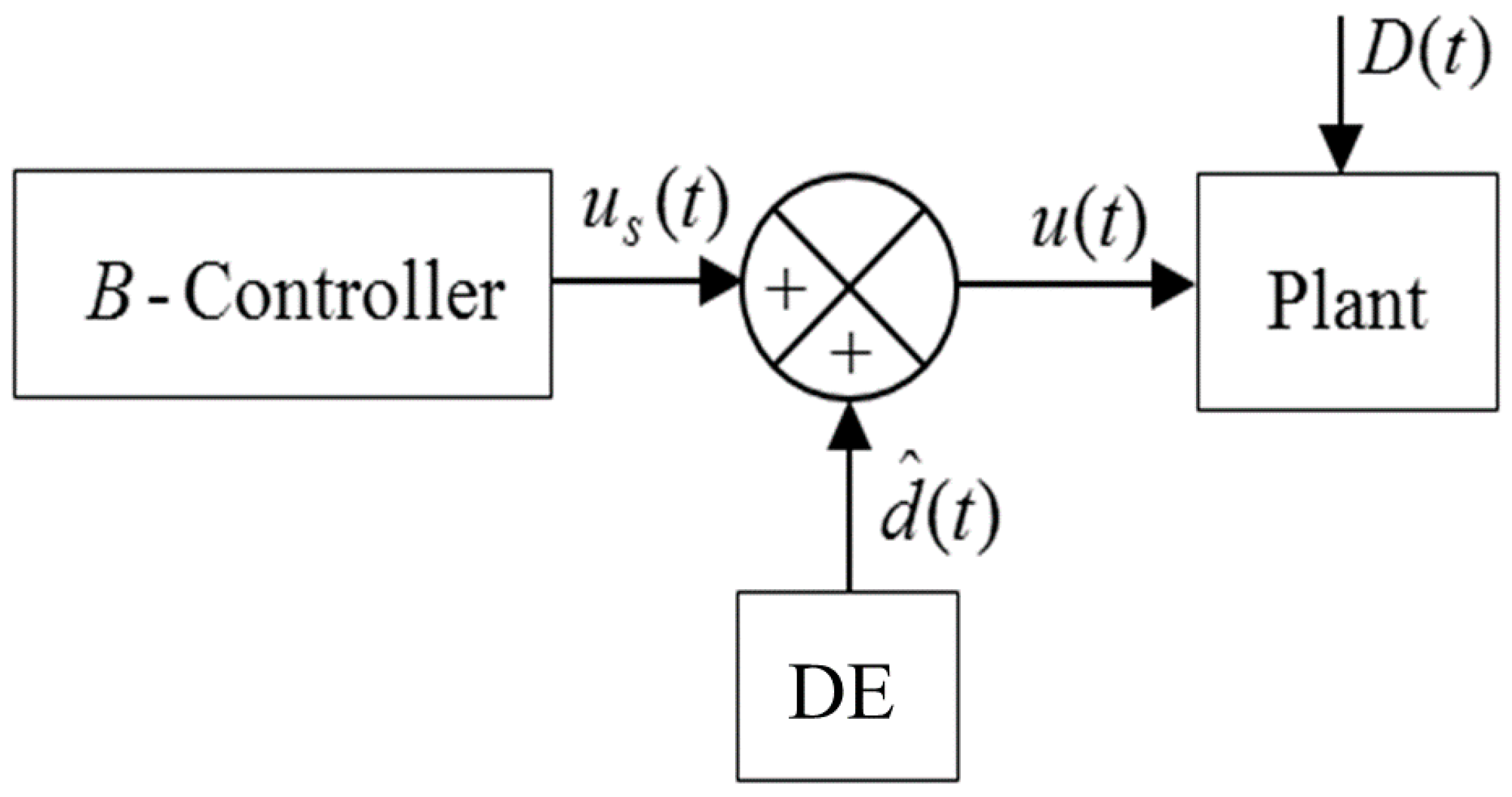
4. Design of Disturbance Estimator

In this section, the disturbance estimator (DE) for d ( t ) in system (2) is designed such that d ^ ( t ) d ( t ) . In order to undertake this, Equation (2) is re-written as follows.
{ x ˙ 1 = x 2 x ˙ n 1 = x n x ˙ n = x ( n ) = f 0 ( x , t ) + g 01 ( x , t ) u ( t ) + g 02 ( t ) d ( t ) y = x 1
In a compact form, this equation is re-written as follows.
{ x ˙ = F ( x , t ) + G 1 ( x , t ) u ( t ) + G 2 ( x , t ) d ( t ) y = x 1 F ( x , t ) = [ x 2 , x 3 , , x n , f 0 ( x , t ) ] T R n G 1 ( x , t ) = [ 0 , , 0 , g 01 ( x , t ) ] T R n G 2 ( x , t ) = [ 0 , , 0 , g 02 ( t ) ) ] T R n .
Then, the estimate d ^ ( t ) is expressed as follows [33].
d ^ ( t ) = z ( x , t ) + l ( x ) x
In the above, a vector of constant parameters l ( x ) needs to be chosen so that the following error function converges to zero.
E ( t ) = d ( t ) d ^ ( t )
In Equation (41), z ( x , t ) is the internal state of the nonlinear observer. The function z ( x , t ) is then estimated as follows:
z ˙ ( x , t ) = l ( x ) ( G 1 ( x , t ) u ( t ) + G 2 ( x , t ) p ( x ) + F ( x , t ) ) l ( x ) G 2 ( x , t ) z ( x , t ) p ( x ) = l ( x ) x .
In order to design DE, consider control system (2), which is re-written as (40). If the estimate d ^ ( t ) given in (41) with a constant parameter vector l ( x ) = [ l 1 , , l n ] is used, then l i ( i = 1 n ) and l n > 0 , E ( t ) 0 when t . Thus, this is a stable process. This can be proved as follows.
Through considering the time derivative of (42) with Equations (41) and (40), the following equation is obtained.
E ˙ ( t ) = d ˙ ( t ) d ^ ˙ ( t ) = d ˙ ( t ) z ˙ ( x , t ) p x x ˙ = d ˙ ( t ) z ˙ ( x , t ) l ( x ) x ˙ = d ˙ ( t ) z ˙ ( x , t ) l ( x ) ( F ( x , t ) + G 1 ( x , t ) u ( t ) + G 2 ( x , t ) d ( t ) )
By substituting z ˙ ( x , t ) from (43) into (44) and taking (42), the following equation is achieved.
E ˙ ( t ) = d ˙ ( t ) + l ( x ) G 2 ( x , t ) ( z ( x , t ) + p ( x ) d ( t ) ) E ˙ ( t ) = d ˙ ( t ) l ( x ) G 2 ( x , t ) E ( t )
If the time varying rate of the uncertainty is low, Equation (45) can be re-written as below.
E ˙ ( t ) + l ( x ) G 2 ( x , t ) E ( t ) 0 . l ( x ) = [ l 1 , , l n ] , l i , i = 1 n , G 2 ( x , t ) = [ 0 , , 0 , g 02 ( t ) ) ] T R n
Thus, Equation (46) becomes the following.
E ˙ ( t ) + l n g 02 ( t ) E ( t ) 0
Due to g 02 ( t ) > 0 , it is inferred from (47) that l n > 0 is the sufficient condition for E ( t ) 0 or d ^ ( t ) d ( t ) when t . It means that l i , i = 1 n , and l n > 0 , E ( t ) 0 is a stable process. Based on this, the DE is designed as follows.
d ^ ( t ) = z ( x , t ) + p ( x ) p ( x ) = i = 1 n l i x i , l i , i = 1 n , l n > 0
z ˙ ( x , t ) = l n g 02 ( t ) z ( x , t ) l ( x ) K ¯ , l ( x ) = [ l 1 , , l n ] , K ¯ = [ x 2 , , x n , ( g 01 ( x , t ) u ( t ) + g 02 ( t ) p ( x ) + f 0 ( x , t ) ) ] T . This makes the system (2) be stable system utilizing the DE. It is remarked that for the vector l ( x ) , if the stable condition of the process is E ( t ) 0 or d ^ ( t ) d ( t ) when t is considered, the conditions l ( x ) = [ 0 , , 0 , l n ] R n and l n > 0 are appropriate options. If both the stable condition and the optimal solution are considered together, the conditions l i , i = 1 n , and l n > 0 should be utilized. The larger value of l n makes the convergent rate increase.

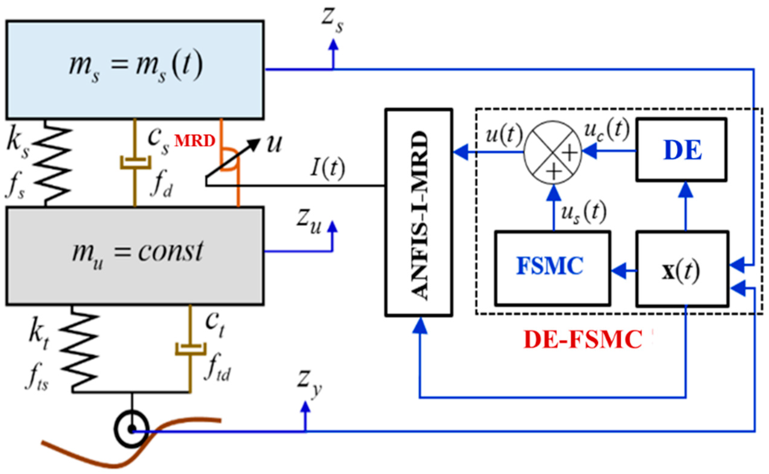
5. Application to Vehicle Suspension System

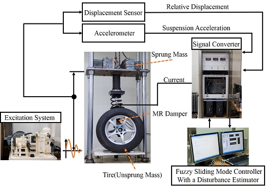
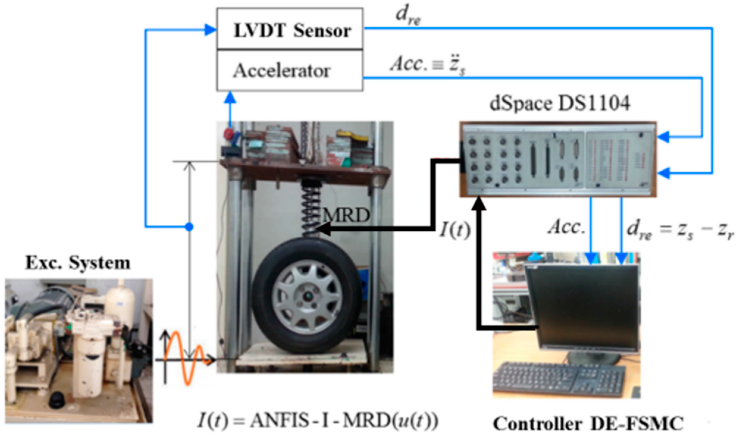
5.1. Experimental Apparatus

Recently, many research works have studied active suspension systems [34,35,36,37] and semi-active suspension systems in order to enhance both ride comfort and road-holding properties. Even though the proposed controller can be applicable to an active suspension system, in this work, the effectiveness of the formulated DE-FSMC is validated by adopting a semi-active vehicle suspension system equipped with a MRD, as shown in Figure 2. The first component is the suspension consisting of a MRD with the damping coefficient c s , and the linear spring with the stiffness coefficient k s . The second component is the controller for damping the force control of the MRD. The third one is the inverse MRD using the adaptive neuro-fuzzy inference system (ANFIS) (named ANFIS-I-MRD). For the car, the chassis mass (also called the sprung mass) m s ( t ) consists of the load, passengers, and impacting factors from the surrounding environment such as the wind force, which is the time-varying parameter. The constant parameter m u denotes the unsprung mass. The vertical displacement of the sprung and unsprung mass are denoted by z s ( t ) and z u ( t ) , respectively, while that of the road profile is denoted by z y ( t ) . It is assumed that the tire deformation is very small, and hence z u ( t ) z r ( t ) . In this test, the disturbance status is expressed by the random change of the chassis mass, m s = 246.5 ± 35 kg. The parameters of the suspension system are given in Table 1. When the suspension system operates, the chassis mass is excited to vibrate due to the vertical vibration of the wheel. In order to reduce the chassis vibration, a current I ( t ) estimated by the controller needs to be applied to the MRD in order to generate required the active force u ( t ) , such that the vibration of the chassis mass is controlled. Hence, the ability of the proposed controller is evaluated via the chassis acceleration. In order to specify I ( t ) via u ( t ) and x ( t ) , the ANFIS-I-MRD needs to be established.
Figure 3 presents a quarter suspension system consisting of four main equipment groups as follows. The suspension system consists of the linear spring k s = 2.8 × 10 4 N/m and the MRD with the damping coefficient of c s = 3000 Ns/m corresponding to the zero current. The hydraulic unit generates excitations with different frequencies and amplitudes. The mechanical structure is constituted of the upper bed, lower bed, and four parallel vertical cylindrical pillars which are used to fix the suspension system, wheel, sprung mass, and sensors. The control system essentially consists of a computer, an analog to digital/digital to analog (AD/DA) converter (dSPASE DS1104, Paderborn, Germany), a current amplifier, and sensors. The sprung mass is set by m s = 246.5 ± 35 kg, including the mass of the upper bed. The relative displacement between the sprung and unsprung mass is measured by LVDT (linear variable differential transformer), while the acceleration of the chassis mass is measured by an accelerometer. The signal from the sensors transmits to the computer via the AD converter. Conversely, the control signal from the computer transmits to the MRD via the DA converter and amplifier to control the damping force.

5.2. Building of ANFIS-I-MRD

The ANFIS-I-MRD is built in two steps. The first step is to build data sets that express the dynamic response of the MRD. The second step is to identify the MRD via the obtained measuring database. For this database, the input–output signal of the i-th data sample is set by [ d r e i v r e i f M R i ] [ I i ] . d r e i = ( z s z r ) i and v r e i = ( z ˙ s z ˙ r ) i denotes relative displacement and velocity between the chassis mass and road. I i is the input current to be supplied to MRD, while f M R i is the produced damping force of the MRD due to the input current. Figure 4 presents the time histories of the filed-dependent damping forces that are to be used as the database. Using this data set and the algorithm for creating ANFIS in a data potential field, named ANFIS-PF [2], a process of training ANFIS is carried out. The trained ANFIS works as the ANFIS-I-MRD in the control system.

5.3. Formulation of DE-FSMC

The controller DE-FSMC is a combination of the B-controller, which directly indicates the FSMC and the DE. With reference to the proposed theory, as well as the structure and operating principle of the suspension system as abovementioned, these two parts are established. The state space model is written as follows.
x ( t ) = [ x 1 , x 2 ] T = [ z s , z ˙ s ] T
From Figure 2, the spring and damping forces are denoted by functions of the displacement and velocity parameters as follows.
f s = k s ( x 1 z r ) ,   f d = c s ( x 2 z ˙ r )
The dynamic response of the sprung mass is then written as below.
{ m s ( t ) z ¨ s + k s ( x 1 z r ) + c s ( x 2 z ˙ r ) = u ( t ) + d ( t ) y = z r
Then, from (51), Equation (1) is re-written for the vehicle suspension system as follows.
{ z s ( 2 ) = f 0 ( x , t ) + g 01 ( x , t ) u ( t ) + g 02 ( t ) D ( t ) y = x 1
f 0 ( x , t ) = 1 m s ( t ) ( k s ( x 1 z r ) + c s ( x 2 z ˙ r ) ) ,   g 01 ( x , t ) = 1 / m s ( t ) ,   g 02 ( t ) = 1 / m s ( t )
By applying Equation (2) to the suspension system, the following equations are obtained.
{ z s ( 2 ) = f ( x , t ) + g 1 ( x , t ) u ( t ) + g 2 ( t ) d ( t ) y = x 1
In the above, g 2 ( t ) = 1 / m s ( t ) . In (52), u ( t ) = u s ( t ) + u c ( t ) , in which control law (20) and update laws (21)–(25) are used to calculate u s ( t ) using the parameters given in Table 2. On the other hand, u c ( t ) is estimated by the DE as follows. It is noted that the values of [ l 1 , l 2 ] are set by [1.51, 24.4] in this work.
x ˙ = [ x ˙ 1 x ˙ 2 ] T = F ( x , t ) + G 1 ( x , t ) u ( t ) + G 2 ( t ) d ( t )
F ( x , t ) = [ x 2 , f 0 ( x , t ) ] T = [ x 2 , ( k s ( x 1 z r ) + c s ( x 2 z ˙ r ) ) / m s ( t ) ] T G 1 ( x , t ) = [ 0 , g 01 ( x , t ) ] T = [ 0 , 1 / m s ( t ) ] T , G 2 ( x , t ) = [ 0 , g 02 ( t ) ] T = [ 0 , 1 / m s ( t ) ] T l ( x ) = [ l 1 , l 2 ] ,   p ( x ) = l 1 x 1 + l 2 x 2 ,   z ˙ ( x , t ) = l 2 g 02 ( t ) z ( x , t ) l ( x ) K ¯ , K ¯ = [ x 2 g 01 ( x , t ) u ( t ) + g 02 ( t ) p ( x ) + f ( x , t ) ]

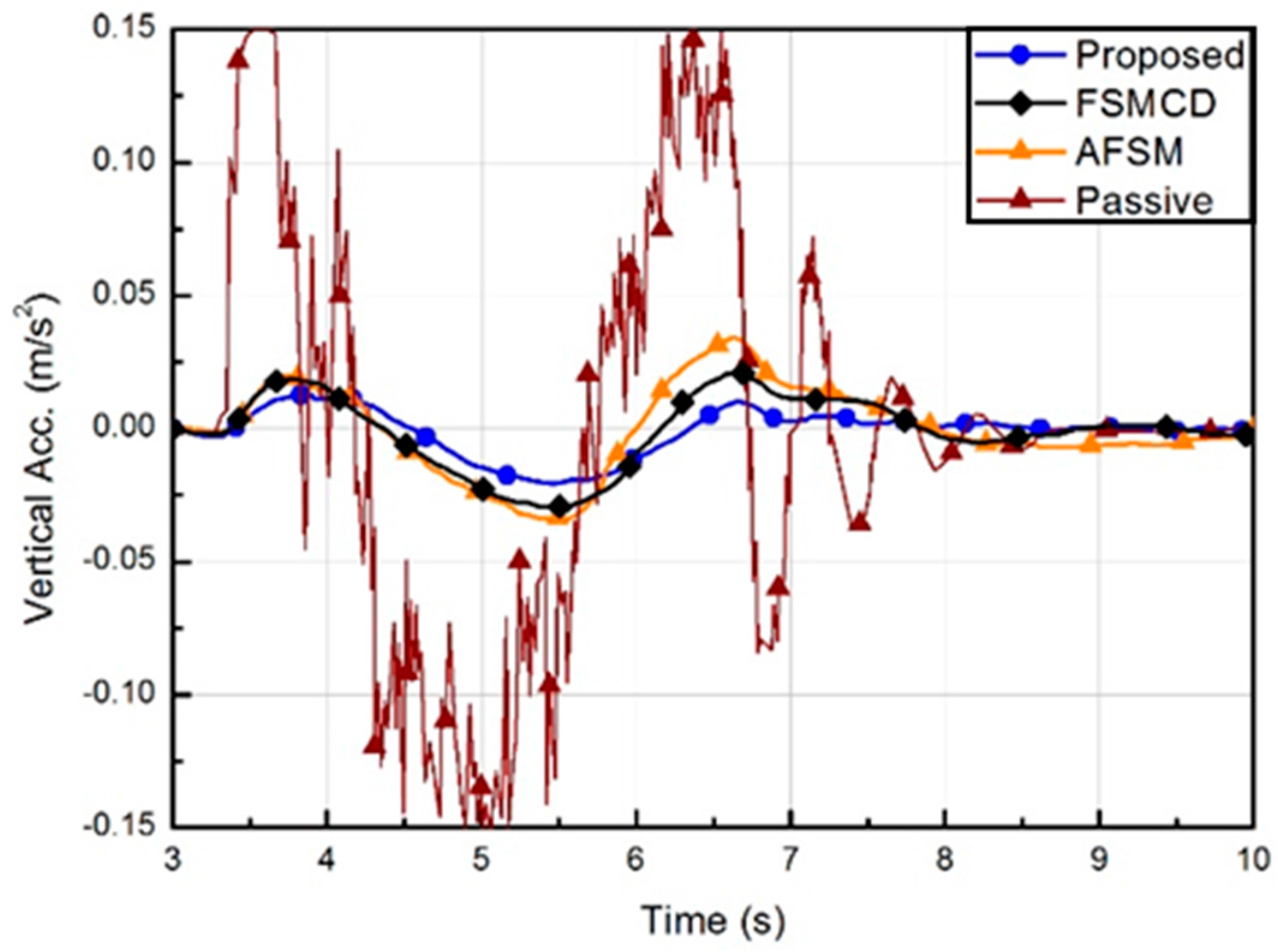
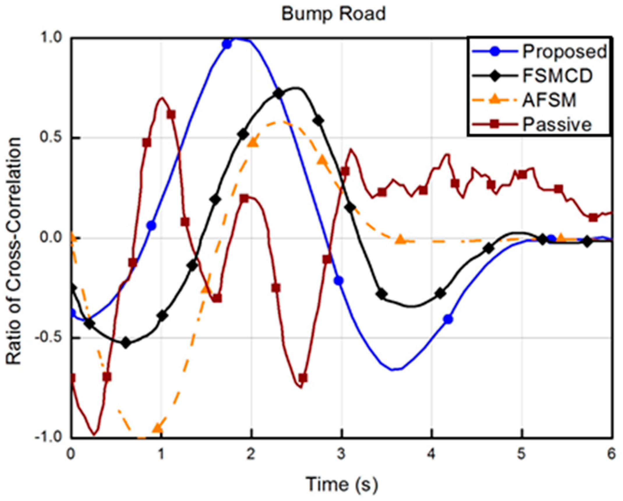
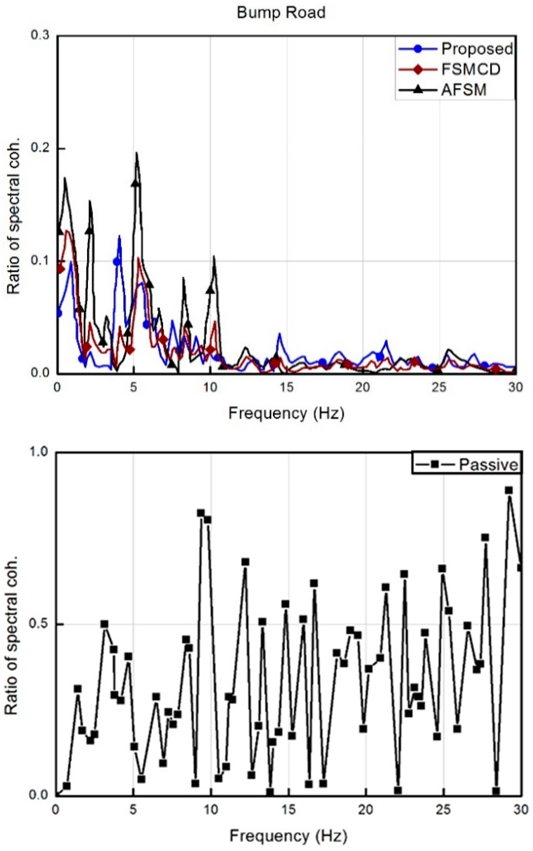
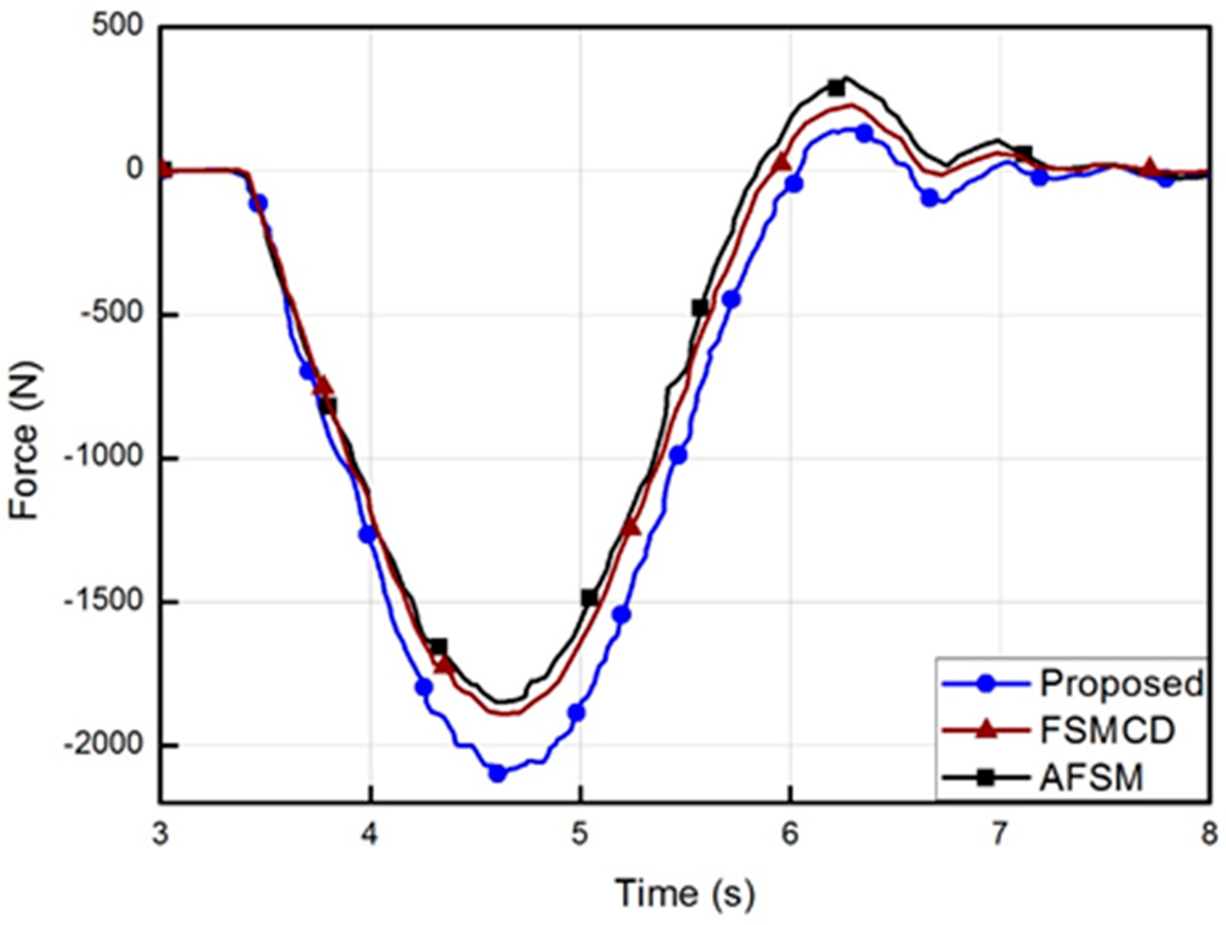
5.4. Results and Discussion

The effectiveness of the proposed DE-FSMC is validated through a comparative work between the proposed controller and an existing adaptive fuzzy sliding mode controller (called the AFSM). For the comparison, the DE-FSMC without the control action (called the passive) and an adaptive fuzzy sliding mode controller proposed in [12] are considered. In this work, in order to show quantitative results, the maximum magnitude of chassis acceleration A a is defined and used.
A a = max i = 1 P | z ¨ s i |
where, P is the number of samples and z ¨ s is the vertical acceleration of the chassis. Two road profiles used for surveys are the bump and sinusoidal type with disturbance surfaces. The MRD is excited to make vibrations with an amplitude of 0.0861 (m) and an angular frequency of 1.9134 (rad/s). It is noted that the speed of the car crossing over the bump profile is decided by 2.34 km/h. The vertical acceleration on the bump road profile is shown in Figure 5. It is identified that the maximum acceleration magnitude A a defined in Equation (80) related to the DE-FSMC is 0.0190 m/s2, which is smaller than that of the fuzzy sliding mode controller with disturbance observer (FSMCD) and AFSM, whose values are 0.0256 and 0.0374 m/s2, respectively. It is noted that the fuzzy sliding mode controller with disturbance observer (FSMCD) used in this work as a comparative controller is the modified one developed in [1], in which the disturbance observer is also used like the proposed one. The AFSM used in this work is the modified one proposed in [30] to adapt to the semi-active suspension system. The numerical results of acceleration identified from the figure are given in Table 3. Figure 6 and Table 3 reflect the dynamic response delay τ between the chassis vertical acceleration signal and the excitation signal coming from the bump-road surface analyzed via cross-correlation function (CCF). The maximum value of τ is identified as 1.869 (s) for the proposed DE-FSMC, while the minimum of τ is calculated by 0.264 (s) for the passive suspension. This indicates that when controlled by the proposed DE-FSMC, the vibration of the chassis is less sensitive to the road surface status compared with the passive AFSM and FSMCD. This is an advantage for controlling vibration by avoiding the resonant status. This aspect is more clearly seen via the ratio of spectral coherence C x y provided in Figure 7 and Table 4. The spectral coherence can identify the frequency-domain correlation between two databases. The values of C x y tending towards zero indicate that the corresponding frequency components are uncorrelated, and conversely for the tending towards 1 [38,39]. For the bump-road profile, C x y between the chassis vertical acceleration signal and the excitation signal coming from the road surface is shown in Figure 7. The maximum values ( C x y max ) and the corresponding frequency ( f C x y max ) related to each method are given in Table 4. The obtained results indicate that the minimum value of C x y max is 0.1269 at the frequency of 4.28 Hz in the proposed method. Besides, f C x y max deriving from the surveyed controllers is located in a narrow range of low frequencies. Figure 8 presents the control force of each controller. It is clearly seen that the proposed controller can provide the better control performance with the similar magnitudes of control force as those of the FSMCD and AFSM.
As a second investigation, the sine-wave road profile is considered as follows [40].
z ( t ) = Z 0 sin ( ω t ) + random ( 0 ; 0.001 ) ( m ) ω = 2 π D V
In this equation, z ( t ) is the vertical displacement of the road surface; Z 0 and D respectively are the amplitude and cycle of the sine-wave; V denotes the velocity of vehicle along the road; and random ( 0 ; 0.001 ) denotes the random value belonging to ( 0.001 , + 0.001 ) . Related to this road profile, random ( 0 ; 0.001 ) indicates the road disturbance surface. By choosing Z 0 = 0.07 m , D = 10 m , and V = 30 km/h, the road profile is achieved, as shown in Figure 9. In order to produce this road profile, an amplitude of 0.07 (m) with an excitation frequency of 0.8333 Hz is used, which is equivalent to the angular frequency of 5.236 rad/s. Figure 10, Figure 11 and Figure 12 and Table 5 and Table 6 present the measured results under the sinusoidal road profile. Figure 10 and Table 5 clearly show that the acceleration of the chassis mass is greatly reduced by activating the proposed controller. The maximum acceleration amplitudes A a of the DE-FSMC, AFSM, and the passive system is identified by 0.3642, 0.5742, 0.7928, and 3.6587 m/s2, respectively. Table 5 shows the dynamic response delay τ between the chassis vertical acceleration signal and the excitation signal coming from the sine-road surface analyzed via CCF. The maximum value of τ is determined by 2.545 (s) from the proposed DE-FSMC, while the minimum of τ is determined by 0.793 (s) from the passive suspension. Figure 11 and Table 6 provide the ratio of spectral coherence C x y , showing its maximum value C x y max , and the corresponding frequency f C x y max related to each method. The minimum value of C x y max is 0.4672 at the frequency of 24.03 Hz in the proposed control method. The required control force corresponding to each controller is shown in Figure 12. It is clearly seen that the vibration control performance of the proposed controller is excellent with the lower input power.

6. Conclusions

In this work, a new adaptive fuzzy sliding mode controller associated with the disturbance estimator (DE-FSMC) was designed, and its effectiveness was validated by adopting the vibration control of a semi-active vehicle suspension system installed with MRD. Firstly, an adaptive control law was formulated based on Lyapunov stability, so that closed-loop stability and finite-time convergence of tracking error could be maintained. Then, a set of solutions for estimating compensative quantity for the impact of UAD on a control system and for avoiding the singular cases of the fuzzy-based function approximation were provided to increase convergence ability and reduce the calculating cost. Subsequently, the effectiveness of the proposed DE-FSMC was verified by undertaking an experimental implementation of the controllers. Vibration control evaluation were investigated under two road profile types; the bump- and sine-typed road with disturbance surfaces, and the following results were achieved.
(1) Vibration control performances under two different road files have verified that the proposed DE-FSMC shows a better performance than the comparative FSMCD and AFSM controllers. Specifically, the maximum acceleration amplitude at the bump road profile is identified by 0.0190, 0.0256, 0.0374 and 0.2394 m/s2 by utilizing the DE-FSMC, FSMCD, AFSM and the passive case, respectively.
(2) It has demonstrated from the cross-correlation function (CCF) that the proposed controller is less sensitive to the excitation signals coming from the road surface status compared with other controllers. Specifically, the minimum value of C x y max (the ratio of spectral coherence) is 0.4672 at the frequency of 24.03 Hz in the proposed control method, while it is 0.5195 in the AFSM under the sinusoidal road profile.
(3) It has been shown that the proposed controller requires the smallest input power in order to achieve excellent vibration control performances. This directly indicates that the updated adaptive control gains determined from the DE-FSMC functionally work well for the semi-active vehicle suspension system featuring MRD dampers.

Acknowledgments

This work was supported by the Incheon National University Research Grant in 2016.

Author Contributions

Byung-Keun Song designed a disturbance estimator and integrated with the main controller and wrote the manuscript, and Jin-Hee An did experimental tests and analyzed the results in terms of vibration control performance. Seung-Bok Choi designed a new control algorithm of the fuzzy sliding mode controller and wrote the manuscript.

Conflicts of Interest

The authors declare that there is no conflict of interest.

References

  1. Nguyen, S.D.; Nguyen, Q.H. Design of active suspension controller for train cars based on sliding mode control, uncertainty observer and neuro-fuzzy system. J. Vib. Control. 2015, 23, 1334–1353. [Google Scholar] [CrossRef]
  2. Nguyen, S.D.; Choi, S.B. Design of a new adaptive neuro-fuzzy inference system based on a solution for clustering in a data potential field. Fuzzy Sets Syst. 2015, 279, 64–86. [Google Scholar] [CrossRef]
  3. Nguyen, S.D.; Nguyen, Q.H.; Choi, S.B. Hybrid clustering based fuzzy structure for vibration control—Part 1: A novel algorithm for building neuro-fuzzy system. Mech. Syst. Signal Process 2014, 50–51, 510–525. [Google Scholar] [CrossRef]
  4. Nguyen, S.D.; Nguyen, Q.H.; Choi, S.B. Hybrid clustering based fuzzy structure for vibration control—Part 2: An application to semi-active vehicle seat-suspension system. Mech. Syst. Signal Process 2014, 56–57, 288–301. [Google Scholar] [CrossRef]
  5. Sivanandan, S.N.; Sumathi, S.; Deepa, S.N. Inductionto Fuzzy Logic Using MATLAB; Springer: Berlin/Heidelberg, Germany, 2007. [Google Scholar]
  6. Castillo, O.; Melin, P. A review on the design and optimization of interval type-2 fuzzy controllers. Appl. Soft Comput. 2012, 12, 1267–1278. [Google Scholar] [CrossRef]
  7. Ginoya, D.; Shendge, P.D.; Phadke, S.B. Disturbance observer based sliding mode control of nonlinear mismatched uncertain systems. Commun. Nonlinear Sci. Numer. Simul. 2015, 26, 98–107. [Google Scholar] [CrossRef]
  8. Deshpande, V.S.; Shendge, P.D.; Phadke, S.B. Active suspension systems for vehicles based on a sliding-mode controller in combination with inertial delay control. Proc. IMechE Part D 2013, 227, 675–690. [Google Scholar] [CrossRef]
  9. Deshpande, V.S.; Mohan, B.; Shendge, P.D.; Phadke, S.B. Disturbance observer based sliding mode control of active suspension systems. J. Sound Vib. 2014, 333, 2281–2296. [Google Scholar] [CrossRef]
  10. Ling, F.X.; Yue, Z. Sliding-mode output feedback control for active suspension with nonlinear actuator dynamics. J. Vib. Control. 2013, 21, 2721–2738. [Google Scholar]
  11. Mahmoodabadi, M.J.; Taherkhorsandi, M.; Talebipour, M.; Castillo-Villar, K.K. Adaptive robust PID control subject to supervisory decoupled sliding mode control based upon genetic algorithm optimization. Trans. Inst. Meas. Control. 2015, 37, 505–514. [Google Scholar] [CrossRef]
  12. Mohammad, R.; Mohammad, H.; Mohammad, R. An optimal and intelligent control strategy for a class of nonlinear systems: Adaptive fuzzy sliding mode. J. Vib. Control. 2014, 22, 159–175. [Google Scholar]
  13. Pan, Y.; Wei, W.; Furuta, K. Hybrid sliding sector control for a wheeled mobile robot. ProcIMechE Part I 2008, 222, 829–837. [Google Scholar] [CrossRef]
  14. Zhang, B.L.; Han, Q.L.; Zhang, X.M.; Yu, X. Sliding Mode Control with Mixed Current and Delayed States for Offshore Steel Jacket Platforms. IEEE Trans. Control. Syst. Technol. 2013, 22, 1769–1783. [Google Scholar] [CrossRef]
  15. Chen, W.H. Disturbance observer based control for nonlinear systems. IEEE/ASME Trans. Mech. 2004, 9, 706–710. [Google Scholar] [CrossRef] [Green Version]
  16. Madoński, R.; Herman, P. Survey on methods of increasing the efficiency of extended state disturbance observers. ISA Trans. 2015, 56, 18–27. [Google Scholar] [CrossRef] [PubMed]
  17. Wu, L.; Wang, C.; Zeng, Q. Observer-based sliding mode control for a class of uncertain nonlinear neutral delay systems. J. Frankl. Inst. 2008, 345, 233–253. [Google Scholar] [CrossRef]
  18. Chan, P.T.; Rad, A.B.; Wang, J. Indirect adaptive fuzzy sliding mode control: Part II: Parameter projection and supervisory control. Fuzzy Sets Syst. 2001, 122, 31–43. [Google Scholar] [CrossRef]
  19. Liang, J.W.; Chen, H.Y.; Wu, Q.W. Active suppression of pneumatic vibration isolators using adaptive sliding controller with self-tuning fuzzy compensation. J. Vib. Control. 2013, 21, 246–259. [Google Scholar] [CrossRef]
  20. Nekoukar, V.; Erfanian, A. Adaptive fuzzy terminal sliding mode control for a class of MIMO uncertain nonlinear systems. Fuzzy Sets Syst. 2011, 179, 34–49. [Google Scholar] [CrossRef]
  21. Oguz, Y.; Hasan, A. Neural based sliding-mode control with moving sliding surface for the seismic isolation of structures. J. Vib. Control. 2011, 17, 2103–2116. [Google Scholar]
  22. Hosseini, R.; Qanadli, S.D.; Barman, S.; Mazinani, M.; Ellis, T.; Dehmeshki, J. An automatic approach for learning and tuning Gaussian interval type-2 fuzzy membership functions applied to lung CAD classification system. IEEE Trans. Fuzzy Syst. 2012, 20, 224–234. [Google Scholar] [CrossRef]
  23. Ho, H.F.; Wong, Y.K.; Rad, A.B. Adaptive fuzzy sliding mode control with chattering elimination for nonlinear SISO systems. Simul. Model. Pract. Theory 2009, 17, 1199–1210. [Google Scholar] [CrossRef]
  24. Yao, J.L.; Shi, W.K. Development of a sliding mode controller for semi-active vehicle suspensions. J. Vib. Control. 2013, 19, 1152–1160. [Google Scholar] [CrossRef]
  25. Li, H.; Yu, J.; Hilton, C.; Liu, H. Adaptive Sliding-Mode Control for Nonlinear Active Suspension Vehicle Systems Using T-S Fuzzy Approach. IEEE Trans. Ind. Electron. 2013, 60, 3328–3338. [Google Scholar] [CrossRef]
  26. Khazaee, M.; Markazi, A.H.D.; Omidi, E. Adaptive fuzzy predictive sliding control of uncertain nonlinear systems with bound-known input delay. ISA Trans. 2015, 59, 314–324. [Google Scholar] [CrossRef] [PubMed]
  27. Mobayen, S.; Javadi, S. Disturbance observer and finite-time tracker design of disturbed third-order nonholonomic systems using terminal sliding mode. J. Vib. Control. 2015, 23, 181–189. [Google Scholar] [CrossRef]
  28. Wang, J.; Rad, A.B.; Chan, P.T. Indirect adaptive fuzzy sliding model control—Part I: Fuzzy switching. Fuzzy Sets Syst. 2001, 122, 21–30. [Google Scholar] [CrossRef]
  29. Geravand, M.; Aghakhani, N. Fuzzy Sliding Mode Control for applying to active vehicle suspensions. WSEAS Trans. Syst. Control. 2010, 5, 48–57. [Google Scholar]
  30. Sharkawy, A.B.; Salman, S.A. An Adaptive Fuzzy Sliding Mode Control Scheme for Robotic Systems. Intell. Control Autom. 2011, 2, 299–309. [Google Scholar] [CrossRef]
  31. Bououden, S.; Chadli, M.; Karimi, H.R. Fuzzy Sliding Mode Controller Design Using Takagi-Sugeno Modelled Nonlinear Systems; Hindawi Publishing Corporation: New York, NY, USA, 2013. [Google Scholar]
  32. Khanesar, M.A.; Kaynak, O.; Yin, S.; Gao, H. Adaptive indirect fuzzy sliding mode controller for networked control systems subject to time-varying network-induced time delay. IEEE Trans. Fuzzy Syst. 2015, 23, 205–214. [Google Scholar] [CrossRef]
  33. Chen, W.H. Nonlinear disturbance observer-enhanced Dynamic inversion control of missiles. J. Guid. Control. Dyn. 2003, 26, 161–166. [Google Scholar] [CrossRef]
  34. Prattichizzo, D.; Mercorelli, P. On some geometric properties of active suspensions systems. Kybernetika 2000, 36, 549–570. [Google Scholar]
  35. Bittanti, S.; Savaresi, S.M. On the parameterization and design of an ex tended Kalman filter frequency tracker. IEEE Trans. Autom. Control. 2000, 45, 1718–1724. [Google Scholar] [CrossRef]
  36. Bittanti, S.; dell Orto, F.; Di Carlo, A.; Savaresi, S.M. Notch filtering and multi-rate control for radial tracking in high-speed dvd-players. IEEE Trans. Consum. Electron. 2002, 48, 56–62. [Google Scholar] [CrossRef]
  37. Savaresi, S.M.; Bittanti, S.; So, H.C. Closed-form unbiased frequency estimation of a noisy sinusoid using notch filters. IEEE Trans. Autom. Control. 2003, 48, 1285–1292. [Google Scholar] [CrossRef]
  38. Gong, W.; Cai, Z. Differential Evolution With Ranking-Based Mutation Operators. IEEE Trans. Cybern. 2013, 43, 1–16. [Google Scholar] [CrossRef] [PubMed]
  39. Bendat, J.; Piersol, A. Engineering Applications of Correlation and Spectral Analysis, 2nd ed.; John Wiley & Sons, Inc.: New York, NY, USA, 1993. [Google Scholar]
  40. Bendat, J.; Piersol, A. Random Data: Analysis and Measurement Procedures, 4nd ed.; John Wiley & Sons, Inc.: New York, NY, USA, 2010. [Google Scholar]
Figure 1. The solution structure: the B-controller, including the estimating uncertainties related to the model error, while the disturbance estimator (DE) for the estimating external disturbances d ( t ) only.
Applsci 07 01053 g001
Figure 2. Control logic associated with the semi-active vehicle suspension system with a magnetorheological damper (MRD). ANFIS: adaptive neuro-fuzzy inference system; FSMC: fuzzy sliding mode controller.
Applsci 07 01053 g002
Figure 3. Experimental apparatus for a quarter vehicle semi-active suspension system with a MRD. LVDT: linear variable differential transformer.
Applsci 07 01053 g003
Figure 4. Database extracted from the measured results.
Applsci 07 01053 g004
Figure 5. Acceleration of the chassis mass m s .
Applsci 07 01053 g005
Figure 6. Ratio of cross-correlation between the chassis vertical acceleration signal and the excitation signal coming from the bump-road profile.
Applsci 07 01053 g006
Figure 7. Spectral coherence C x y between the excitation signal coming from the bump-typed road surface and acceleration signal of the chassis-mass.
Applsci 07 01053 g007
Figure 8. Control force u ( t ) corresponding to each controller.
Applsci 07 01053 g008
Figure 9. The sine wave road profile with a disturbance surface.
Applsci 07 01053 g009
Figure 10. Acceleration of the chassis mass under two different sine-road excitations.
Applsci 07 01053 g010
Figure 11. Ratio of cross-correlation between the chassis vertical acceleration signal and the excitation signal.
Applsci 07 01053 g011
Figure 12. Control force corresponding to each controller.
Applsci 07 01053 g012
Table 1. The principal parameters of the suspension system.
m s = 246.5 ± 35 kg
k s = 2.8 × 10 4 N/m
c s = 3000 Ns/m
Table 2. Parameters of the fuzzy sliding mode controller (FSMC).
Sliding Surface S = 10 e + e ˙
η 1 1.51
η 2 1.73
Φ 1
Ω 0 150
x d = [ x 1 , x 2 ] T = [ z s , z ˙ s ] T [ 0 , 0 ] T
Number of fuzzy laws49
Table 3. Bump road: the maximum acc. and time delay of acc. response. AFSM: adaptive fuzzy sliding mode; FSMCD: fuzzy sliding mode controller with disturbance observer.
Controller A a (m/s2) τ (s)
Proposed0.01901.869
FSMCD0.02561.321
AFSM0.03740.905
Passive0.23940.264
Table 4. Bump road: the maximum value of C x y and the corresponding frequency.
Controller A a (m/s2) τ (s)
Proposed0.12694.28
FSMCD0.19855.05
AFSM0.21755.45
Passive0.920847.08
Table 5. Sine road: the acceleration and time delay.
Controller A a (m/s2) τ (s)
Proposed0.36422.545
AFSM0.57421.359
Passive3.65870.793
Table 6. Sine road: the spectral coherence at corresponding frequency.
Controller C x y max f C x y max (Hz)
Proposed0.467224.03
AFSM0.519570.54
Passive0.814089.92

