
Nondestructive Estimation of Moisture Content, pH and Soluble Solid Contents in Intact Tomatoes Using Hyperspectral Imaging

 ,
, 

Abstract
:1. Introduction
2. Materials and Methods
2.1. Tomato Samples
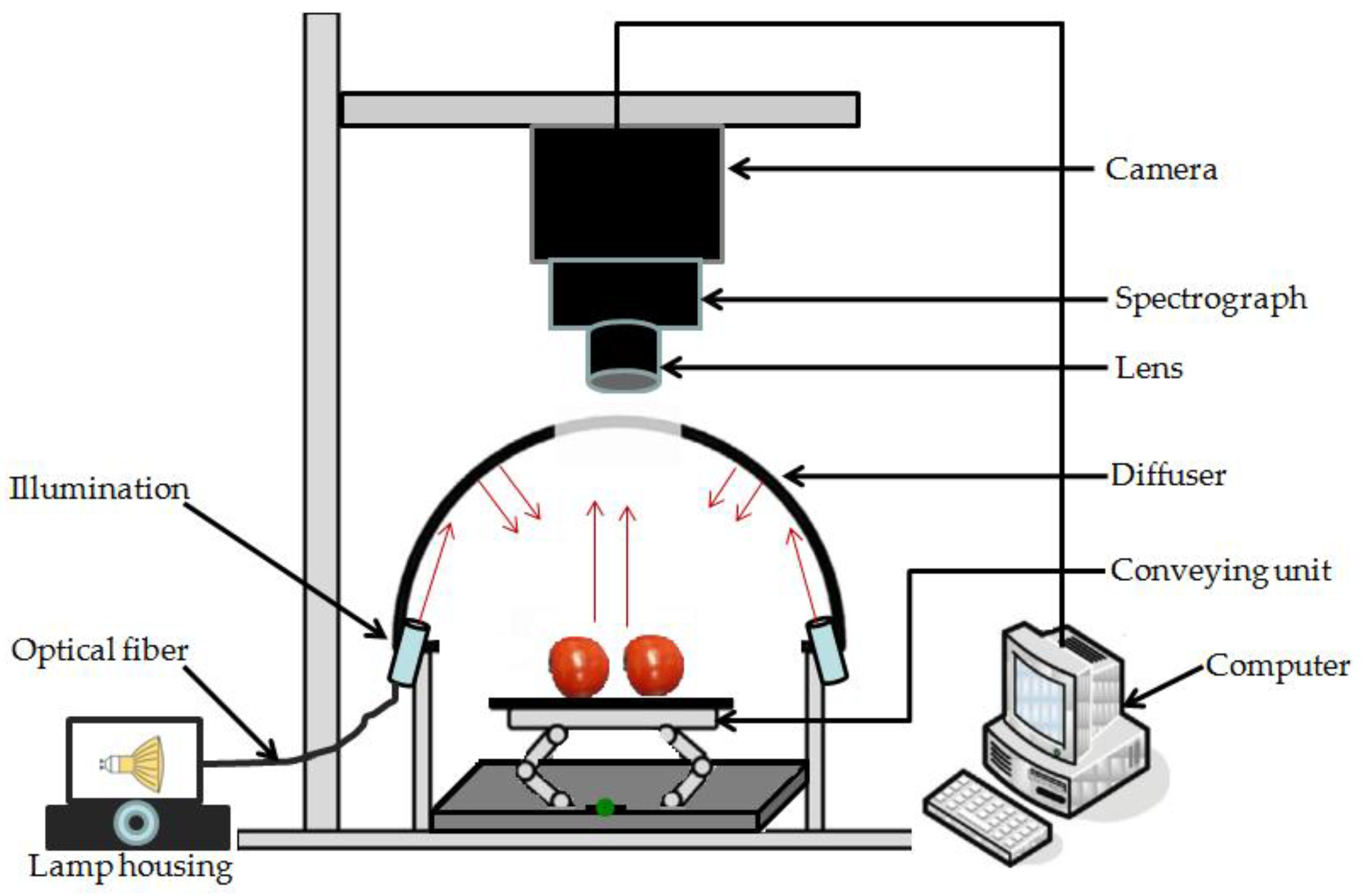
2.2. Hyperspectral Imaging System
2.3. Image Correction
2.4. Spectra Data Extraction
2.5. Reference Measurements
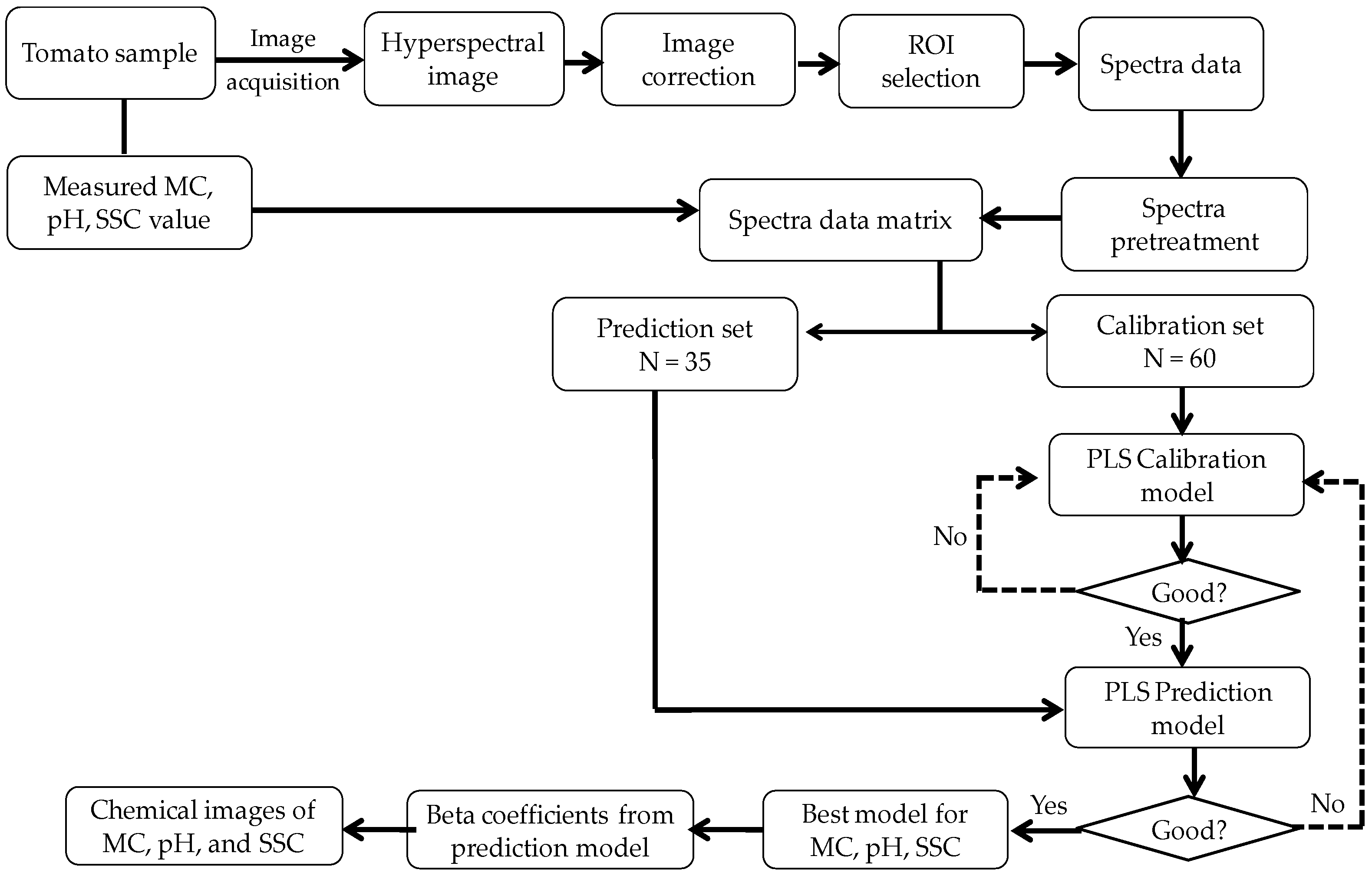
2.6. Data Analysis
2.6.1. Spectral Preprocessing
2.6.2. Development of Calibration Model
2.6.3. Evaluation of the Calibration and Prediction Models
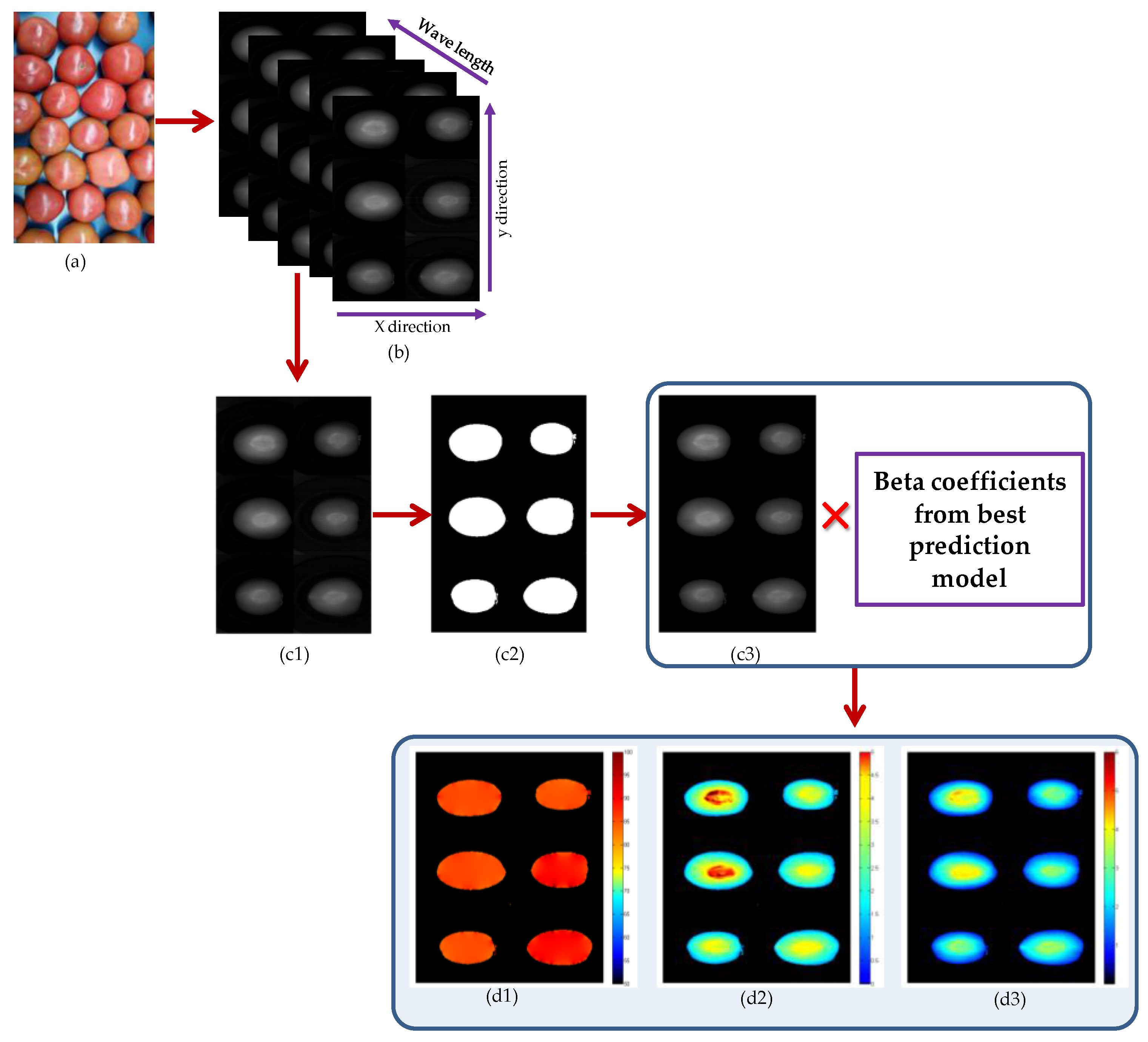
2.6.4. Chemical Images of MC, pH, and SSC in Intact Tomatoes
3. Results and Discussions
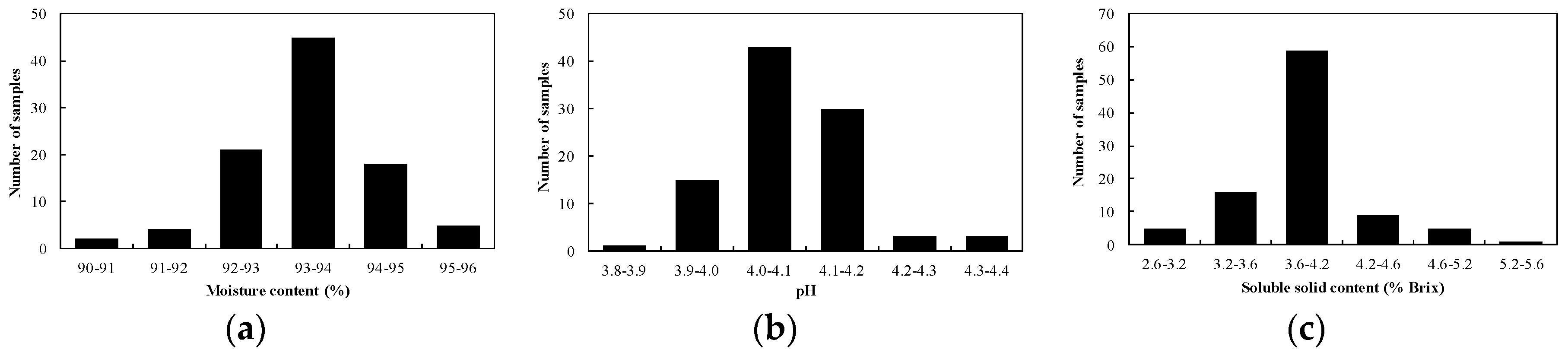
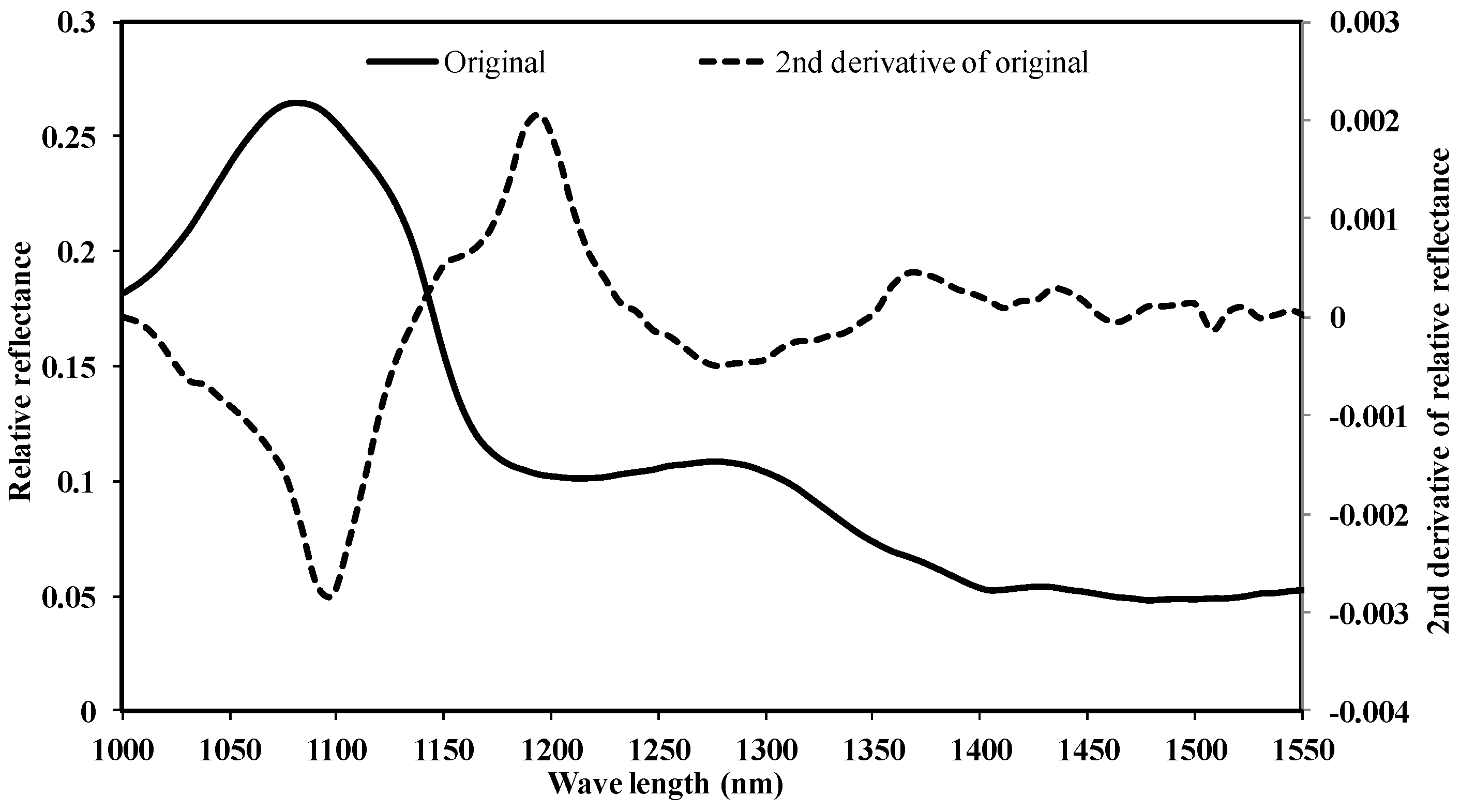
3.1. Overview of Spectral Features and Statistics of Reference Analysis
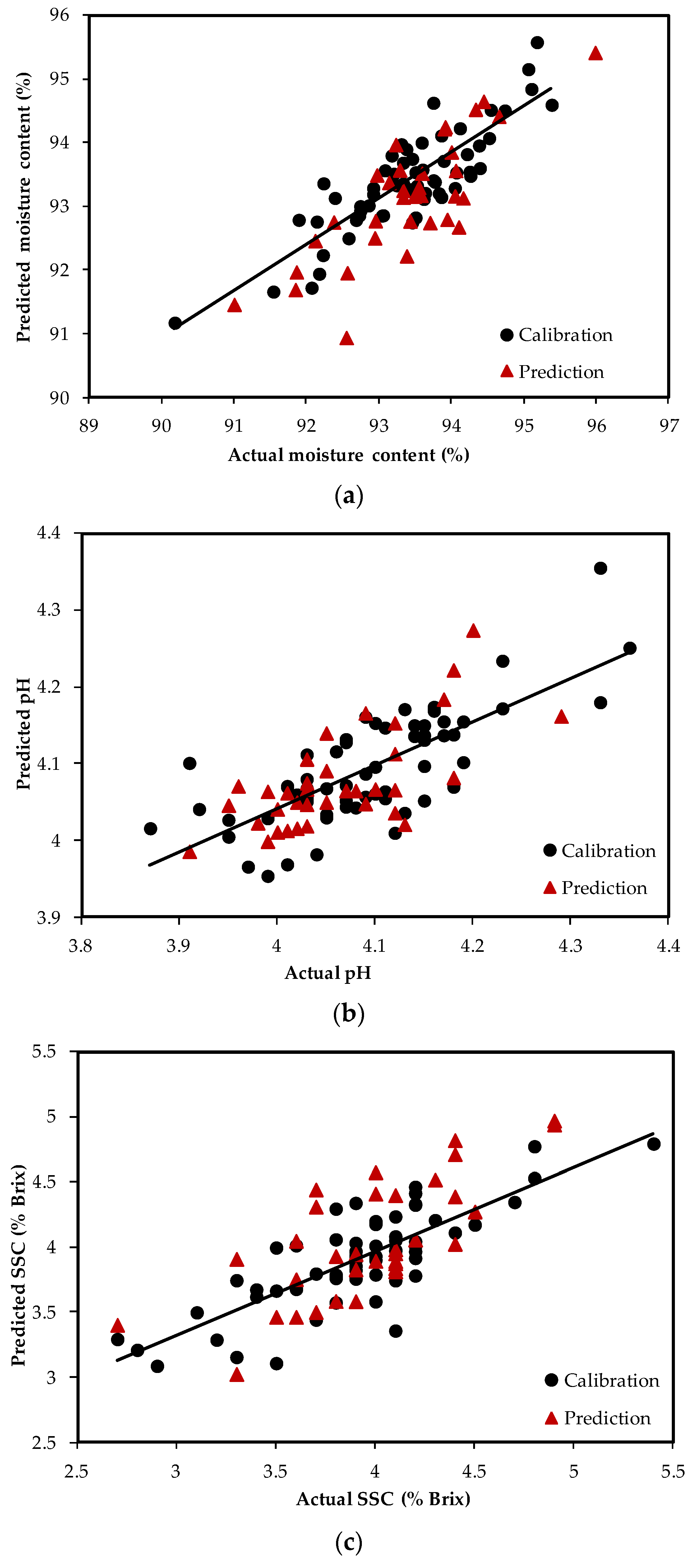
3.2. PLS Regression Models
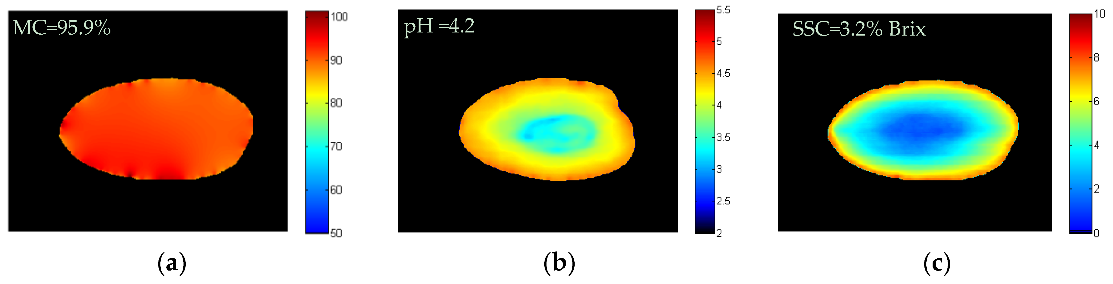
3.3. Chemical Images of MC, pH and SSC in Intact Tomatoes
4. Conclusions
Acknowledgments
Author Contributions
Conflicts of Interest
References
- FAOSTAT: Food and Agriculture Organiztion of the United Nations Statistics Division. Available online: http://www.fao.org/faostat/en/#data/QC/visualize (accessed on 10 November 2016).
- Bhowmik, D.; Sampath Kumar, K.P.; Paswan, S.; Srivastava, S. Tomato—A natural medicine and its health benefits. J. Pharmacogn. Phytochem. 2012, 1, 33–43. [Google Scholar]
- Petcharaporn, K.; Kumchoo, S. Calibration model of %titratable acidity (citric acid) for intact tomato by transmittance SW-NIR spectroscopy. Int. J. Biol. Biomol. Agric. Food Biotechnol. Eng. 2014, 8, 825–828. [Google Scholar]
- Mollazade, K.; Omid, M.; Tab, F.A.; Mohtasebi, S.S.; Zude, M. Spatial mapping of noisture content in tomato fruits using hyperspectral imaging and artificial neural networks. In Proceedings of the CIGR-AgEng2012: IV International workshop on Computer Image Analysis in Agriculture, Valencia, Spain, 8–12 July 2012.
- Amigo, J.M.; Martí, I.; Gowen, A. Hyperspectral imaging and chemometrics: A perfect combination for the analysis of food Structure, composition and quality. Data Handl. Sci. Technol. 2013, 28, 343–370. [Google Scholar]
- Qin, J.; Chao, K.; Kim, M.S.; Lu, R.; Burks, T.F. Hyperspectral and multispectral imaging for evaluating food safety and quality. J. Food Eng. 2013, 118, 157–171. [Google Scholar] [CrossRef]
- Mohammadi Moghaddam, T.; Razavi, S.M.A.; Taghizadeh, M. Applications of hyperspectral imaging in grains and nuts quality and safety assessment: A review. J. Food Meas. Charact. 2013, 7, 129–140. [Google Scholar] [CrossRef]
- Wu, D.; Sun, D.-W. Advanced applications of hyperspectral imaging technology for food quality and safety analysis and assessment: A review—Part I: Fundamentals. Innov. Food Sci. Emerg. Technol. 2013, 19, 1–14. [Google Scholar] [CrossRef]
- Huang, M.; Wan, X.; Zhang, M.; Zhu, Q. Detection of insect-damaged vegetable soybeans using hyperspectral transmittance image. J. Food Eng. 2013, 116, 45–49. [Google Scholar] [CrossRef]
- ElMasry, G.; Wang, N.; ElSayed, A.; Ngadi, M. Hyperspectral imaging for nondestructive determination of some quality attributes for strawberry. J. Food Eng. 2007, 81, 98–107. [Google Scholar] [CrossRef]
- Rajkumar, P.; Wang, N.; EImasry, G.; Raghavan, G.S.V.; Gariepy, Y. Studies on banana fruit quality and maturity stages using hyperspectral imaging. J. Food Eng. 2012, 108, 194–200. [Google Scholar] [CrossRef]
- Huang, M.; Wang, Q.; Zhang, M.; Zhu, Q. Prediction of color and moisture content for vegetable soybean during drying using hyperspectral imaging technology. J. Food Eng. 2014, 128, 24–30. [Google Scholar] [CrossRef]
- Gowen, A.A.; O’Donnell, C.P.; Taghizadeh, M.; Gaston, E.; O’Gorman, A.; Cullen, P.J.; Frias, J.M.; Esquerre, C.; Downey, G. Hyperspectral imaging for the investigation of quality deterioration in sliced mushrooms (Agaricus bisporus) during storage. Sens. Instrum. Food Qual. Saf. 2008, 2, 133–143. [Google Scholar] [CrossRef]
- Sivakumar, S.S. Potential Applications of Hyperspectral Imaging for the Determination of Total Soluble Solids, Water Content and Firmness in Mango. Master’s Thesis, McGill University, Montreal, QC, Canada, 2006. [Google Scholar]
- Li, X.; He, Y. Non-destructive measurement of acidity of Chinese bayberry using Vis/NIRS techniques. Eur. Food Res. Technol. 2006, 223, 731–736. [Google Scholar] [CrossRef]
- Baiano, A.; Terracone, C.; Peri, G.; Romaniello, R. Application of hyperspectral imaging for prediction of physico-chemical and sensory characteristics of table grapes. Comput. Electron. Agric. 2012, 87, 142–151. [Google Scholar] [CrossRef]
- Nogales-Bueno, J.; Hernández-Hierro, J.M.; Rodríguez-Pulido, F.J.; Heredia, F.J. Determination of technological maturity of grapes and total phenolic compounds of grape skins in red and white cultivars during ripening by near infrared hyperspectral image: A preliminary approach. Food Chem. 2014, 152, 586–591. [Google Scholar] [CrossRef] [PubMed]
- Noh, H.K.; Lu, R. Hyperspectral laser-induced fluorescence imaging for assessing apple fruit quality. Postharvest Biol. Technol. 2007, 43, 193–201. [Google Scholar] [CrossRef]
- Leiva-Valenzuela, G.A.; Lu, R.; Aguilera, J.M. Prediction of firmness and soluble solids content of blueberries using hyperspectral reflectance imaging. J. Food Eng. 2013, 115, 91–98. [Google Scholar] [CrossRef]
- Mendoza, F.; Lu, R.; Ariana, D.; Cen, H.; Bailey, B. Integrated spectral and image analysis of hyperspectral scattering data for prediction of apple fruit firmness and soluble solids content. Postharvest Biol. Technol. 2011, 62, 149–160. [Google Scholar] [CrossRef]
- Schmilovitch, Z.; Ignat, T.; Alchanatis, V.; Gatker, J.; Ostrovsky, V.; Felföldi, J. Hyperspectral imaging of intact bell peppers. Biosyst. Eng. 2014, 117, 83–93. [Google Scholar] [CrossRef]
- Kandpal, L.M.; Lee, S.; Kim, M.S.; Bae, H.; Cho, B.-K. Short wave infrared (SWIR) hyperspectral imaging technique for examination of aflatoxin B1 (AFB1) on corn kernels. Food Control 2015, 51, 171–176. [Google Scholar] [CrossRef]
- Rahman, A.; Kondo, N.; Ogawa, Y.; Suzuki, T.; Shirataki, Y.; Wakita, Y. Prediction of K value for fish flesh based on ultraviolet-visible spectroscopy of fish eye fluid using partial least squares regression. Comput. Electron. Agric. 2015, 117, 149–153. [Google Scholar] [CrossRef]
- Cen, H.; He, Y. Theory and application of near infrared reflectance spectroscopy in determination of food quality. Trends Food Sci. Technol. 2007, 18, 72–83. [Google Scholar] [CrossRef]
- Downey, G.; Robert, P.; Bertrand, D.; Kelly, P.M. Classification of commercial skim milk powders according to heat treatment using factorial discriminant analysis of near-infrared reflectance spectra. Appl. Spectrosc. 1990, 44, 150–155. [Google Scholar] [CrossRef]
- Swierenga, H.; de Weijer, A.P.; van Wijk, R.J.; Buydens, L.M.C. Strategy for constructing robust multivariate calibration models. Chemom. Intell. Lab. Syst. 1999, 49, 1–17. [Google Scholar] [CrossRef]
- Chen, H.; Song, Q.; Tang, G.; Feng, Q. The combined optimization of Savitzky-Golay smoothing and multiplicative scatter correction for FT-NIR PLS models. ISRN Spectrosc. 2013, 2013, 642190. [Google Scholar] [CrossRef]
- Barnes, R.J.; Dhanoa, M.S.; Lister, S.J. Standard Normal Variate Transformation and De-trending of Near-Infrared Diffuse Reflectance Spectra. Appl. Spectrosc. 1989, 43, 772–777. [Google Scholar] [CrossRef]
- Candolfi, A.; De Maesschalck, R.; Jouan-Rimbaud, D.; Hailey, P.A.; Massart, D.L. The influence of data pre-processing in the pattern recognition of excipients near-infrared spectra. J. Pharm. Biomed. Anal. 1999, 21, 115–132. [Google Scholar] [CrossRef]
- Camps, C.; Christen, D. On-tree follow-up of apricot fruit development using a hand-held NIR instrument. J. Food Agric. Environ. 2009, 7, 394–400. [Google Scholar]
- Gómez, A.H.; He, Y.; Pereira, A.G. Non-destructive measurement of acidity, soluble solids and firmness of Satsuma mandarin using Vis/NIR-spectroscopy techniques. J. Food Eng. 2006, 77, 313–319. [Google Scholar] [CrossRef]
- Kamruzzaman, M.; Makino, Y.; Oshita, S. Hyperspectral imaging for real-time monitoring of water holding capacity in red meat. LWT Food Sci. Technol. 2016, 66, 685–691. [Google Scholar] [CrossRef]
- Kamruzzaman, M.; ElMasry, G.; Sun, D.-W.; Allen, P. Non-destructive prediction and visualization of chemical composition in lamb meat using NIR hyperspectral imaging and multivariate regression. Innov. Food Sci. Emerg. Technol. 2012, 16, 218–226. [Google Scholar] [CrossRef]
- He, Y.; Zhang, Y.; Pereira, A.G.; Gómez, A.H.; Wang, J. Nondestructive determination of tomato fruit quality characteristics using VIS/NIR spectroscopy technique. Int. J. Inf. Technol. 2005, 11, 97–108. [Google Scholar]
- Li, J.; Tian, X.; Huang, W.; Zhang, B.; Fan, S. Application of long-wave near infrared hyperspectral imaging for measurement of soluble solid content (SSC) in pear. Food Anal. Methods 2016, 9, 3087–3098. [Google Scholar] [CrossRef]


| Items | MC (%) | pH | SSC (% Brix) | |||
|---|---|---|---|---|---|---|
| Calibration | Prediction | Calibration | Prediction | Calibration | Prediction | |
| No. of samples | 60 | 35 | 60 | 35 | 60 | 35 |
| Maximum value | 95.9 | 94.4 | 4.4 | 4.3 | 5.5 | 4.9 |
| Minimum value | 91.0 | 91.2 | 3.9 | 3.9 | 2.7 | 3.4 |
| Mean ± SD | 93.6 ± 0.94 | 93.4 ± 0.92 | 4.1 ± 0.1 | 4.1 ± 0.08 | 3.9 ± 0.47 | 3.9 ± 0.44 |
| Parameter | Preprocessing Method | No. of LVs | Calibration | Prediction | ||
|---|---|---|---|---|---|---|
| rcal | RMSEC | rpred | RMSEP | |||
| MC | Raw | 7 | 0.81 | 0.44 | 0.79 | 0.56 |
| Smoothing (moving average) a | 8 | 0.87 | 0.45 | 0.79 | 0.65 | |
| Max normalization | 7 | 0.88 | 0.44 | 0.71 | 5.74 | |
| Mean normalization | 6 | 0.84 | 0.51 | 0.76 | 0.64 | |
| Range normalization | 7 | 0.86 | 0.48 | 0.77 | 0.62 | |
| S–G first derivatives b | 6 | 0.85 | 0.50 | 0.81 | 0.63 * | |
| S–G second derivatives b | 9 | 0.88 | 0.45 | 0.71 | 0.69 | |
| MSC c | 5 | 0.83 | 0.52 | 0.74 | 0.66 | |
| SNV d | 5 | 0.81 | 0.54 | 0.73 | 0.67 | |
| pH | Raw | 3 | 0.72 | 0.06 | 0.65 | 0.06 |
| Smoothing (moving average) a | 3 | 0.75 | 0.06 | 0.71 | 0.06 | |
| Max normalization | 2 | 0.33 | 0.09 | 0.50 | 0.08 | |
| Mean normalization | 2 | 0.32 | 0.09 | 0.50 | 0.08 | |
| Range normalization | 2 | 0.32 | 0.09 | 0.49 | 0.08 | |
| S–G first derivatives b | 2 | 0.75 | 0.06 | 0.69 | 0.06 * | |
| S–G second derivatives b | 2 | 0.76 | 0.06 | 0.67 | 0.06 | |
| MSC c | 2 | 0.32 | 0.09 | 0.37 | 0.08 | |
| SNV d | 2 | 0.32 | 0.09 | 0.37 | 0.08 | |
| SSC | Raw | 7 | 0.82 | 0.24 | 0.63 | 0.33 |
| Smoothing (moving average) a | 5 | 0.80 | 0.28 | 0.74 | 0.33 * | |
| Max normalization | 6 | 0.80 | 0.28 | 0.53 | 0.41 | |
| Mean normalization | 6 | 0.80 | 0.28 | 0.55 | 0.40 | |
| Range normalization | 6 | 0.79 | 0.29 | 0.54 | 0.39 | |
| S– first derivatives b | 7 | 0.78 | 0.30 | 0.65 | 0.36 | |
| S–G second derivatives b | 6 | 0.64 | 0.36 | 0.50 | 0.39 | |
| MSC c | 5 | 0.78 | 0.29 | 0.55 | 0.40 | |
| SNV d | 5 | 0.77 | 0.30 | 0.47 | 0.42 | |
© 2017 by the authors; licensee MDPI, Basel, Switzerland. This article is an open access article distributed under the terms and conditions of the Creative Commons Attribution (CC BY) license (http://creativecommons.org/licenses/by/4.0/).
Share and Cite
Rahman, A.; Kandpal, L.M.; Lohumi, S.; Kim, M.S.; Lee, H.; Mo, C.; Cho, B.-K. Nondestructive Estimation of Moisture Content, pH and Soluble Solid Contents in Intact Tomatoes Using Hyperspectral Imaging. Appl. Sci. 2017, 7, 109. https://doi.org/10.3390/app7010109
Rahman A, Kandpal LM, Lohumi S, Kim MS, Lee H, Mo C, Cho B-K. Nondestructive Estimation of Moisture Content, pH and Soluble Solid Contents in Intact Tomatoes Using Hyperspectral Imaging. Applied Sciences. 2017; 7(1):109. https://doi.org/10.3390/app7010109
Chicago/Turabian StyleRahman, Anisur, Lalit Mohan Kandpal, Santosh Lohumi, Moon S. Kim, Hoonsoo Lee, Changyeun Mo, and Byoung-Kwan Cho. 2017. "Nondestructive Estimation of Moisture Content, pH and Soluble Solid Contents in Intact Tomatoes Using Hyperspectral Imaging" Applied Sciences 7, no. 1: 109. https://doi.org/10.3390/app7010109
APA StyleRahman, A., Kandpal, L. M., Lohumi, S., Kim, M. S., Lee, H., Mo, C., & Cho, B.-K. (2017). Nondestructive Estimation of Moisture Content, pH and Soluble Solid Contents in Intact Tomatoes Using Hyperspectral Imaging. Applied Sciences, 7(1), 109. https://doi.org/10.3390/app7010109