A Simple Predator-Prey Population Model with Rich Dynamics

Abstract

A non-smooth switched harvest on predators is introduced into a simple predator-prey model with logistical growth of the prey and a bilinear functional response. If the density of the predator is below a switched value, the harvesting rate is linear; otherwise, it is constant. The model links the well studied predator-prey model with constant harvesting to that with a proportional harvesting rate. It is shown that when the net reproductive number for the predator is greater than unity, the system is permanent and there may exist multiple positive equilibria due to the effects of the switched harvest, a saddle-node bifurcation, a limit cycle, and the coexistence of a stable equilibrium and a unstable circled inside limit cycle and a stable circled outside limit cycle. When the net reproductive number is less than unity, a backward bifurcation from a positive equilibrium occurs, which implies that the stable predator-extinct equilibrium may coexist with two coexistence equilibria. In this situation, reducing the net reproductive number to less than unity is not enough to enable the predator to go extinct. Numerical simulations are provided to illustrate the theoretical results. It seems that the model possesses new complex dynamics compared to the existing harvesting models.

1. Introduction

Mathematical modeling of predator-prey interactions have attracted wide attention since the original work by Lotka and Volterra in 1920s, and there have been extensively studied for their rich dynamics [1,2,3]. Since the rich and complex dynamics for interactive species are common in the real world, many researchers have investigated the processes that affect the dynamics of prey-predator models and wanted to know what models can best represent species interactions.

As a simplest form, the interaction between a predator and prey may be modeled by a pair of differential equations [1,3,4,5],

$$\begin{array}{c}{\displaystyle \frac{dN}{dt}=rN(1-\frac{N}{K})-aNP}\hfill \\ {\displaystyle \frac{dP}{dt}=caNP-dP}\hfill \end{array}$$

(1)

where N and P represent the prey and predator species, respectively; $r,K,a,c$, and d are positive constants. In the absence of the predation, the prey grows logistically with intrinsic growth rate r and carrying capacity K. In the presence of the predator, the prey species decreases at a rate proportional to the functional response $aN$, where a presents the rate of predation. The factor c denotes the efficiency of predation which divides a maximum per capita birth rate of the predators into a maximum per capita consumption rate. Without the prey, no predation occurs and the predator species decreases exponentially with mortality rate d.

To consider the dynamics of model Equation (1), it is shown that the origin $(0,0)$ is a saddle point. Define the net reproductive number of the predator population $n_0$, i.e., the expected number of a predator individual producing as the predator population is introduced into a stable prey population [6,7], as

$$n_0={\displaystyle \frac{caK}{d}}$$

(2)

Then if $n_0<1$, the boundary equilibrium $(K,0)$ with the predator going extinct is globally asymptotically stable and there exists no positive equilibrium for the prey-predator interaction. If $n_0>1$, the boundary equilibrium $(K,0)$ is a saddle point and there exists a positive coexistence equilibrium $(N_{*},P_{*})=\left(\frac{K}{n_0},\frac{r}{a}\left(1-\frac{1}{n_0}\right)\right)$, which is globally asymptotically stable. The model dynamics are relatively simple. Using $n_0$ as bifurcation parameter, we have a transcritical bifurcation at $n_0=1$ as $(N_{*},P_{*})$ is bifurcated. Notice that model Equation (1) is a special case of the prey-predator model in [8].

Apparently, model Equation (1) fails to show the complicated dynamics of the predator-prey interactions in the real world. Later, many researchers improve and enrich model Equation (1) by incorporating some other elements, for example, stage-structure [9,10,11,12,13], nonlinear functional response function [14,15,16,17,18], dispersal among patchers [19], delays [9,10,11,20], or impulsive effects [18,21].

In the real world, from the point of view of predators’ needs, the exploitation of biological resources and harvest are commonly practiced in fishery, forestry, and wildlife management. There is an interest in the use of bioeconomic models to gain insight into the scientific management of renewable resources [16]. Moreover, harvesting is an important and effective method to prevent and control the explosive growth of predators or prey when they are enough. So, generally speaking, it is reasonable and necessary for one to introduce the harvest of populations into models. Taking the above reasons into a consideration, we focus on the predator-prey model with harvest [12,13,16,17,20,21,22,23,24,25,26,27,28].

Normally, harvesting has several forms in predator-prey models. The most common one of these harvesting forms is a nonzero constant [16,17,20,22,23,24,26] or a linear harvesting rate [12,13,22,25,26,27,28]. In Ref. [22], a two-prey-one-predator model with predator harvested was studied. The authors are particularly interested in the stability properties of different harvest strategies. Two types of harvest strategies are: with a nonzero constant and a linear harvesting rate. The choice of idealized harvest strategies will contribute to a qualitative understanding of the properties of different harvesting strategies. Xiao and Jennings [16] considered the dynamical properties of the ratio-dependent predator-prey model with constant prey harvesting. There existed numerous kinds of bifurcations, such as the saddle-node bifurcation, the subcritical and supercritical Hopf bifurcations. There also existed a limit cycle, a homoclinic or heteroclinic orbit satisfying different parameter values. In Ref. [17], the ratio-dependent predator-prey model with constant predator harvesting was focused on. Philip et al. [26] also discussed two predator-prey models with linear or nonzero constant predator harvesting.

The above two types of harvesting rates seemingly have their own advantages as well as disadvantages in fitting the harvest in the real world. When the density of the predator or prey is rather low, the nonzero constant harvesting rate is not as reasonable as of the proportional type [13,22,26]; while if the predator or prey is abundant, linear harvesting rate is less possible than the constant harvesting rate [16]. In Ref. [22], to compare the stability properties of the system with two harvest strategies, they applied linear or constant harvesting rate, respectively. In that comparative study, the authors demonstrated that switching from linear to constant harvesting rate may turn a stable stationary state to a periodic or chaotic oscillatory mode from a mathematical perspective. However, when deciding the constant level of harvesting, the instability of the constant harvest strategy calls for great care. In Ref. [29], Beddington et al. introduced a more realistic smooth harvesting function in which the fishing effort is limited upwards because the constant harvest cannot be achieved for small populations of the fish. The adjustment of a harvesting function can prevent extinction and increase the stability to some extent. Moreover, the dramatic increase of the predator or prey challenges the normal ecological balance and capacity of harvest. Thus, it is interesting to construct a new kind of harvesting rate that combines the advantages from both linear and constant harvesting rates.

Motivated by these ideas, in this paper, we consider a predator-prey model with a novel harvesting rate. Our ideas to develop the harvesting rate are derived from the capacity of treatments of diseases that had been well studied in the dynamical epidemic models [30,31,32].

Using model Equation (1) as our baseline model, we assume that harvesting takes place, but only the predator population is under harvesting and introduce harvesting function $H\left(P\right)$ of the predator to prey-predator model Equation (1) for discussing its dynamical features. The interactive dynamics are governed by the following system

$$\begin{array}{cc}{\displaystyle \frac{dN}{dt}}=\hfill & rN\left(1-\frac{N}{K}\right)-aNP\hfill \\ {\displaystyle \frac{dP}{dt}}=\hfill & caNP-dP-H\left(P\right)\hfill \end{array}$$

(3)

Following the methods in [14,15,16,17,30], we investigate the existence and stability of multiple equilibria, bifurcations, and limit cycles, and study the effects of switched harvest on the dynamics of the predator-prey model.

This paper is organized as follow. Section 2 and Section 3.1 represent the boundedness of model Equation (3) and existence of multiple equilibria. In Section 3.2, we study the stability of equilibria, bifurcations, and the existence and stability of a limit cycle. In Section 4, we give numerical simulations to verify our results. Brief discussions are presented finally in Section 5.

2. Model Formulation

Now, we consider model Equation (3). Firstly, we describe harvesting function $H\left(P\right)$ of the predators in model Equation (3), which has the following form

$$H\left(P\right)=\left\{\begin{array}{c}mP,0\le P\le P_0\hfill \\ h,P_0<P\hfill \end{array}\right.$$

(4)

We assume that the harvesting rate is proportional to the predator population size until it reaches a threshold value due to limited facilities of harvesting or resource protection. The harvesting rate will then be kept as a constant. Denote the harvesting threshold value as $h=m{P}_0$.

When $0\le P\le P_0$, model Equation (3) is

$$\begin{array}{cc}{\displaystyle \frac{dN}{dt}}=\hfill & rN\left(1-\frac{N}{K}\right)-aNP\hfill \\ {\displaystyle \frac{dP}{dt}}=\hfill & caNP-dP-mP\hfill \end{array}$$

(5)

When $P>P_0$, model Equation (3) becomes

$$\begin{array}{cc}{\displaystyle \frac{dN}{dt}}=\hfill & rN\left(1-\frac{N}{K}\right)-aNP\hfill \\ {\displaystyle \frac{dP}{dt}}=\hfill & caNP-dP-h\hfill \end{array}$$

(6)

It is straightforward to verify that solutions of Equation (3) with positive initial conditions are all positive for $t\ge 0$ and ultimately bounded. Thus the following set

$$D=\left\{(N,P):N\ge 0,P\ge 0,cN+P\le \frac{ck{(r+d)}^2}{4rd}\right\}$$

is positive invariant for system Equation (3).

3. Preliminary Results

3.1. Existence of Equilibria

In this section, we explore the existence of all nonnegative equilibria. First, the origin $(0,0)$ is still a trivial equilibrium and the predator-free equilibrium $(K,0)$ exists. Moreover, it is easy to see that there exists no positive equilibrium in region D if $n_0\le 1$. We thus assume $n_0>1$ hereafter, and present our results of the existence of positive equilibria as follows.

Theorem 1. 

System Equation (3) has a positive coexistence equilibrium $E^{*}(N^{*},P^{*})$, in the subregion of D with $0<P\le P_0$,

$$N^{*}={\displaystyle \frac{K}{\widehat{n}}},P^{*}={\displaystyle \frac{r}{a}}\left(1-{\displaystyle \frac{1}{\widehat{n}}}\right)$$

(7)

if and only if $P_0\ge {\displaystyle \frac{r}{a}}$ and $\widehat{n}>1$, or $P_0<{\displaystyle \frac{r}{a}}$ and $1<\widehat{n}\le {\displaystyle \frac{r}{r-a{P}_0}}$, where ${\displaystyle \frac{r}{a}}$ represents the maximum predator density for which the prey population can establish itself from a small initial population and $\widehat{n}$ is the net reproductive number of the predator under harvesting defined by

$$\widehat{n}=\frac{caK}{d+m}$$

(8)

Proof. 

In the subregion of D with $0<P\le P_0$, a positive equilibrium of Equation (3) satisfies

$$\left\{\begin{array}{c}r{N}^{*}\left(1-\frac{N^{*}}{K}\right)-a{N}^{*}{P}^{*}=0\hfill \\ ca{N}^{*}{P}^{*}-(d+m)P^{*}=0\hfill \end{array}\right.$$

(9)

Then it follows that

$$N^{*}=\frac{d+m}{ca}={\displaystyle \frac{K}{\widehat{n}}}$$

and then

$$P^{*}={\displaystyle \frac{r}{a}}\left(1-{\displaystyle \frac{1}{\widehat{n}}}\right)>0$$

if $\widehat{n}>1$. In the mean time, it follows from

$$P^{*}={\displaystyle \frac{r}{a}}\left(1-{\displaystyle \frac{1}{\widehat{n}}}\right)\le P_0$$

and then

$${\displaystyle \frac{1}{\widehat{n}}}\ge {\displaystyle \frac{r-a{P}_0}{r}}$$

that there exists a positive equilibrium in this subregion if

$${\displaystyle \frac{r-a{P}_0}{r}}\le 0$$

or if ${\displaystyle \frac{r-a{P}_0}{r}}>0$ and

$$\widehat{n}\le {\displaystyle \frac{1}{1-\frac{a{P}_0}{r}}}={\displaystyle \frac{r}{r-a{P}_0}}$$

(10)

   ☐

To investigate the existence of positive equilibria in the subregion of D with $P>P_0$, we first give the relation of roots and coefficients for a quadratic equation.

Quadratic equation $(x-A)(B-x)=C$, with constants A, B, and C positive, has two positive roots

$$x_1={\displaystyle \frac{A+B-\sqrt{{(B-A)}^2-4C}}{2}}<x_2={\displaystyle \frac{A+B+\sqrt{{(A-B)}^2-4C}}{2}}$$

a unique positive root

$$x={\displaystyle \frac{A+B}{2}}$$

or no positive root, if

$$C<{\displaystyle \frac{{(B-A)}^2}{4}},C={\displaystyle \frac{{(B-A)}^2}{4}},\mathrm{or}C>{\displaystyle \frac{{(B-A)}^2}{4}}$$

respectively.

The results for the existence of positive equilibria of Equation (3) in the subregion of D with $P>P_0$ are provided as follows.

Theorem 2. 

We assume $P_0<{\displaystyle \frac{r}{a}}$ and define

$$\widehat{P}={\displaystyle \frac{r(n_0-1)}{2a{n}_0}},h_1={\displaystyle \frac{crK}{4}}{\left(1-{\displaystyle \frac{1}{n_0}}\right)}^2,h_2={\displaystyle \frac{rm}{a}}\left(1-{\displaystyle \frac{1}{\widehat{n}}}\right)$$

(11)

System Equation (3), in the subregion of D with $P>P_0$, has

(a) 

No positive equilibrium if

$$h>h_1,or\left\{\begin{array}{c}{P}_0>\widehat{P}\hfill \\ h_2\le h<h_1\hfill \end{array}\right.$$

(b) 

A unique positive equilibrium with

$$N={\displaystyle \frac{K(1+n_0)}{2n_0}},P={\displaystyle \frac{r(K-N)}{aK}}={\displaystyle \frac{r(n_0-1)}{2a{n}_0}}$$

(12)

if

$$h=h_1,\left\{\begin{array}{c}{P}_0>\widehat{P},\hfill \\ h<h_{1}andh<h_2\hfill \end{array}\right.or\left\{\begin{array}{c}{P}_0<\widehat{P},\hfill \\ h<h_{1}andh\le h_2\hfill \end{array}\right.$$

(c)

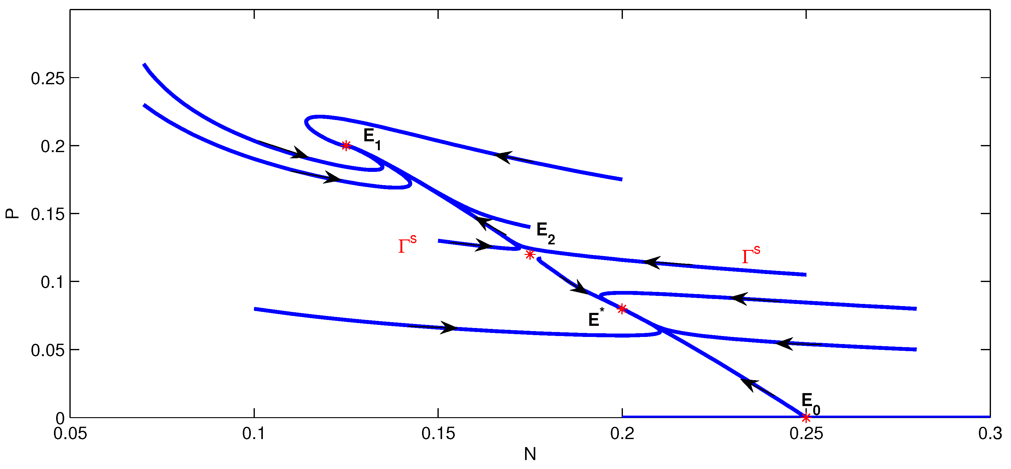
Two positive equilibria $E_i(N_i,P_i)$, $i=1,2$, where

$$\begin{array}{cc}\hfill N_1=& {\displaystyle \frac{crK(1+n_0)-n_0\sqrt{4crK\left(h_1-h\right)}}{2cr{n}_0}}\hfill \\ & <{\displaystyle \frac{crK(1+n_0)+n_0\sqrt{4crK\left(h_1-h\right)}}{2cr{n}_0}}=N_2\hfill \end{array}$$

(13)

and

$$P_2={\displaystyle \frac{r(K-N_2)}{aK}}<P_1={\displaystyle \frac{r(K-N_1)}{aK}}$$

if $h<h_1$ and

$$\left\{\begin{array}{c}{P}_0<\widehat{P}\hfill \\ \widehat{n}<1\hfill \end{array}\right.or\left\{\begin{array}{c}{P}_0<\widehat{P}\hfill \\ h_2<h\hfill \end{array}\right.$$

Proof. 

In the subregion of D with $P>P_0$, a positive equilibrium satisfies

$$\begin{array}{c}\hfill rN(1-\frac{N}{K})-aNP=0\end{array}$$

(14a)

$$\begin{array}{c}\hfill caNP-dP-h=0\end{array}$$

(14b)

It follows from Equation (14a) that

$$P={\displaystyle \frac{r(K-N)}{aK}}$$

Substituting it into Equation (14b) yields

$$\left(N-{\displaystyle \frac{K}{n_0}}\right)(K-N)={\displaystyle \frac{K}{cr}}h$$

(15)

It follows from the relation of roots and coefficients for the quadratic equation $(x-A)(B-x)=c$ shown above that equation Equation (15) has no, unique, or two positive solutions if $h>h_1$, $h=h_1$, or $h<h_1$.

To have $P_i>P_0$, $i=1,2$, we need

$$P_i={\displaystyle \frac{r(K-N_i)}{aK}}>P_0$$

that is,

$$N_i<K-{\displaystyle \frac{aK}{r}}{P}_0={\displaystyle \frac{aK}{r}}\left({\displaystyle \frac{r}{a}}-P_0\right),i=1,2$$

(16)

Thus, if $P_0\ge r/a$, there is no positive equilibrium of Equation (15) in the subregion of D with $P>P_0$. We assume $P_0<r/a$.

Suppose there are two positive solutions, $N_1<N_2$, to Equation (15) and hence $P_2<P_1$. Then $P_2>P_0$ if and only if

$$N_2<K-{\displaystyle \frac{aK}{r}}{P}_0$$

(17)

Substituting $N_2$ in Equation (13) into Equation (17) yields

$$n_0\sqrt{4crK\left(h_1-h\right)}<crK(n_0-1)-2caK{n}_0{P}_0$$

that is,

$${\displaystyle \frac{\sqrt{4crK}}{2caK}}\sqrt{\left(h_1-h\right)}<{\displaystyle \frac{r(n_0-1)}{2a{n}_0}}-P_0=\widehat{P}-P_0$$

(18)

Then if $P_0\ge \widehat{P}$, we have $P_2\le P_0$.

Assume $P_0<\widehat{P}$. Squaring both sides of Equation (18) yields

$${\displaystyle \frac{r}{c{a}^{2}K}}(h_1-h)<{\displaystyle \frac{r^2{(n_0-1)}^2}{4a^2{n}_0^2}}-{\displaystyle \frac{r(n_0-1)}{a{n}_0}}{P}_0+P_0^2$$

(19)

It follows from the definition of $h_1$ that

$${\displaystyle \frac{r{h}_1}{c{a}^{2}K}}={\displaystyle \frac{r}{c{a}^{2}K}}{\displaystyle \frac{crK{(n_0-1)}^2}{4n_0^2}}={\displaystyle \frac{r^2{(n_0-1)}^2}{4a^2{n}_0^2}}$$

Then Equation (19) becomes

$$\begin{array}{cc}\hfill 0<& h^2-{\displaystyle \frac{rm}{a}}\left({\displaystyle \frac{n_0-1}{n_0}}-{\displaystyle \frac{m}{caK}}\right)h=\left(h-{\displaystyle \frac{rm}{a}}\left(1-{\displaystyle \frac{d+m}{caK}}\right)\right)h\hfill \\ \hfill =& \left(h-{\displaystyle \frac{rm}{a}}\left(1-{\displaystyle \frac{1}{\widehat{n}}}\right)\right)h\hfill \end{array}$$

(20)

If $\widehat{n}<1$, we have $P_2>P_0$. Otherwise, Equation (20) is equivalent to

$$0<(h-h_2)h$$

Thus, if $h_2<h<h_1$, $P_2>P_0$, and if $h\le h_2$, $P_2<P_0$.

We now consider $P_1>P_0$, that is,

$$N_1<{\displaystyle \frac{aK}{r}}\left({\displaystyle \frac{r}{a}}-P_0\right)$$

(21)

Substituting $N_1$ in Equation (13) into Equation (21), we have

$${\displaystyle \frac{\sqrt{4crK}}{2caK}}\sqrt{\left(h_1-h\right)}>P_0-\widehat{P}$$

(22)

If $P_0\le \widehat{P}$, inequality Equation (21) is satisfied which implies $P_1>P_0$.

Suppose $P_0>\widehat{P}$. Similarly as above, inequality Equation (22) is equivalent to

$$0>(h-h_2)h$$

Thus, if $h<h_2$, $P_1>P_0$, and if $h\ge h_2$, $P_1<P_0$.

By putting all together, the proof is completed.   ☐

Remark 1. 

System Equation (1) with linear predator harvest strategy leads to the predator extinct if the net reproductive number $\widehat{n}<1$. However, by Theorem 2 $\left(c\right)$, we find that for system Equation (1) with switched predator harvest strategy; that is, when the density of predator is below harvest level $P_0$, the linear harvesting rate is applied to the system, whereas when the density of predators is higher than harvest level, the system adopts nonzero constant harvesting rate, even if $\widehat{n}<1$, the prey and predator may coexist.

3.2. Stability of Equilibria

In this section, we discuss the stability of equilibria of model Equation (3).

Theorem 3. 

Equilibrium $E_0(K,0)$ is locally asymptotically stable if $\widehat{n}<1$, and unstable if $\widehat{n}>1$. Moreover, $E_0(K,0)$ is globally asymptotically stable in $D\backslash \left\{\right(0,0\left)\right\}$ if $\widehat{n}<1$ and $h>h_1$. If $\widehat{n}>1$, system Equation (3) is permanent.

Proof. 

It is easy to obtain that the characteristic roots to the linearized equation of system Equation (3) at $E_0(K,0)$ are ${\lambda }_1=-r<0$ and ${\lambda }_2=caK-d-m=(d+m)(\widehat{n}-1)$. Thus, $E_0$ is locally asymptotically stable if $\widehat{n}<1$ and unstable if $\widehat{n}>1$.

Next, note that $(0,0)$ is always unstable. If $\widehat{n}<1$, by Theorems 1 and 2, there is not any other equilibrium of system Equation (3) than $E_0$ in $D\backslash \left\{\right(0,0\left)\right\}$. Since D is the invariant set of system Equation (3) and $E_0$ is locally asymptotically stable, it follows from the Bendixson Theorem that every solution of system Equation (3) in D approaches $E_0$ when t tends to positive infinity.

Since $E_0$ is unstable as $\widehat{n}>1$, following the similar arguments to Cantrell and Cosner ([33] Theorem 3.1) (see also ([34] Theorems 3,4)), which is based on the uniform persistence theory introduced by Hale and Waltman [35], we are able to conclude that system Equation (3) is permanent if $\widehat{n}>1$.

The proof is complete.   ☐

Remark 2. 

It follows from Cantrell and Cosner ([33] Theorem 3.1) that system Equation (5) is permanent if and only if $\widehat{n}>1$. Thus Theorem 3 suggests that if system Equation (5) is permanent, then so is system Equation (3).

For the three positive equilibria $E^{*},E_1,E_2$, we have the following results. Firstly, we consider the stability of $E^{*}$.

Theorem 4. 

The positive equilibrium $E^{*}(N^{*},P^{*})$ of system Equation (3) is globally asymptotically stable if $P_0<{\displaystyle \frac{r}{a}}$ and $1<\widehat{n}\le {\displaystyle \frac{r}{r-a{P}_0}}$.

Proof. 

According to Theorem 1, positive equilibrium $E^{*}(N^{*},P^{*})$ exists if and only if $P_0<{\displaystyle \frac{r}{a}}$ and $1<\widehat{n}\le {\displaystyle \frac{r}{r-a{P}_0}}$. The Jacobian matrix of system Equation (3) at $E^{*}(N^{*},P^{*})$ is

$$J^{*}=\left(\begin{array}{cc}r(1-\frac{N^{*}}{K})+r{N}^{*}(-\frac{1}{K})-a{P}^{*}& -a{N}^{*}\\ ca{P}^{*}& ca{N}^{*}-d-m\end{array}\right)$$

(23)

Because $N^{*}$ and $P^{*}$ satisfy Equation (9), by means of Equation (9), the trace and determinant of $J^{*}$ are simplified as

$$\begin{array}{c}{\displaystyle tr(J^{*})=r-\frac{2r{N}^{*}}{K}-a{P}^{*}+ca{N}^{*}-d-m=-\frac{r{N}^{*}}{K}<0}\hfill \\ {\displaystyle det\left(J^{*}\right)=(r-\frac{2r{N}^{*}}{K}-a{P}^{*})(ca{N}^{*}-d-m)+c{a}^2{N}^{*}{P}^{*}=c{a}^2{N}^{*}{P}^{*}>0}\hfill \end{array}$$

(24)

Therefore, all eigenvalues of matrix $J^{*}$ have negative real parts when $P_0<{\displaystyle \frac{r}{a}}$ and $1<\widehat{n}\le {\displaystyle \frac{r}{r-a{P}_0}}$. It follows that $E^{*}(N^{*},P^{*})$ is locally asymptotically stable.

Then, it suffices for us to prove the global attractiveness of $E^{*}(N^{*},P^{*})$. Inspired by the work of McCluskey [36], we define a Lyapunov function

$$M\left(t\right)=c{N}^{*}(\frac{N\left(t\right)}{N^{*}}-ln\frac{N\left(t\right)}{N^{*}}-1)+P^{*}(\frac{P\left(t\right)}{P^{*}}-ln\frac{P\left(t\right)}{P^{*}}-1)$$

where $N^{*}=\frac{K}{\widehat{n}}$, and $P^{*}=\frac{r}{a}(1-\frac{1}{\widehat{n}})$.

We know that $\frac{N\left(t\right)}{N^{*}}-ln\frac{N\left(t\right)}{N^{*}}-1$ and $\frac{P\left(t\right)}{P^{*}}-ln\frac{P\left(t\right)}{P^{*}}-1\ge 0$ for all $N\left(t\right),P\left(t\right)>0$. (The equality holds if and only if $N\left(t\right)=N^{*},P\left(t\right)=P^{*}$.) From the definition of $M\left(t\right)$, we know that $M\left(t\right)$ is well-defined and $M\left(t\right)\ge 0$. The equality holds if and only if $N\left(t\right)=N^{*}$ and $P\left(t\right)=P^{*}$.

Differentiating $M\left(t\right)$ along the solutions of system Equation (3), we obtain

$$\begin{array}{cc}{\displaystyle \frac{dM\left(t\right)}{dt}}\hfill & {\displaystyle =c(1-\frac{N^{*}}{N})\frac{dN}{dt}+(1-\frac{P^{*}}{P})\frac{dP}{dt}.}\hfill \\ & {\displaystyle =-\frac{cr}{K}{N}^2+\frac{2rN(d+m)}{aK}-\frac{r{(d+m)}^2}{c{a}^{2}K}.}\hfill \\ & {\displaystyle =-\frac{cr}{K}{(N-\frac{d+m}{ca})}^2\le 0}\hfill \end{array}$$

It follows that $M\left(t\right)$ is bounded and non-increasing. Thus ${lim}_{t\to \infty }M\left(t\right)$ exists. Note that $\frac{dM}{dt}=0$ if and only if $N=N^{*}$. Substituting $N=N^{*}$ into the first equation of Equation (3), one can directly get $P=P^{*}$. Therefore, the maximal compact invariant set in $\frac{dM}{dt}=0$ is the singleton $E^{*}$. By the LaSalle invariance principle (see, for example, Theorem 5.3.1 in Hale and Verduyn Lunel [37]), positive equilibrium $E^{*}$ is globally attracting. Further, $E^{*}$ is globally asymptotically stable.   ☐

Now we concentrate on the stability of coexistence equilibria $E_i(N_i,P_i)$, $i=1,2$. The Jacobian matrix of system Equation (3), at $E_i(N_i,P_i)$, is

$$J_i=\left(\begin{array}{cc}r-\frac{2r{N}_i}{K}-a{P}_i& -a{N}_i\\ ca{P}_i& ca{N}_i-d\end{array}\right),i=1,2$$

(25)

Theorem 5. 

If the coexistence equilibrium $E_2(N_2,P_2)$ of system Equation (3) exists, it is unstable.

Proof. 

For the coexistence equilibrium $E_2(N_2,P_2)$, $N_2$ and $P_2$ satisfy Equation (14). By Equations (13)–(15), after direct calculations, the determinant of matrix $J_2$ is

$$\begin{array}{c}{\displaystyle det\left(J_2\right)=-\frac{2car}{K}{(N_2-\frac{d+caK}{4ca})}^2+\frac{2car{(d+caK)}^2}{16c^2{a}^{2}K}}\hfill \end{array}$$

(26)

Because

$$N_2={\displaystyle \frac{crK(1+n_0)+n_0\sqrt{4crK(h_1-h)}}{2cr{n}_0}}>{\displaystyle \frac{crK(1+n_0)}{2cr{n}_0}}=\frac{caK+d}{2ca}$$

we obtain that $det\left(J_2\right)<0$. Thus $E_2(N_2,P_2)$ is a saddle point and unstable.   ☐

For the coexistence equilibrium $E_1(N_1,P_1)$, similarly, the determinant of $J_1$ is

$$\begin{array}{c}{\displaystyle det\left(J_1\right)=-\frac{2car}{K}{(N_1-\frac{d+caK}{4ca})}^2+\frac{2car{(d+caK)}^2}{16c^2{a}^{2}K}}\hfill \end{array}$$

(27)

but since

$$N_1={\displaystyle \frac{crK(1+n_0)-n_0\sqrt{4crK(h_1-h)}}{2cr{n}_0}}<{\displaystyle \frac{crK(1+n_0)}{2cr{n}_0}}=\frac{caK+d}{2ca}$$

we obtain $det\left(J_1\right)>0$, and $E_1(N_1,P_1)$ may be node, focus or center.

By Equations (13)–(15), the sign of the trace of matrix $J_1$ is determined by

$$\begin{array}{c}\phi =r^{2}d(d-caK)+2c{a}^{2}K(caK-r)h-ard\sqrt{4crK(h_1-h)}\hfill \end{array}$$

(28)

According to Equation (28), we obtain

(a)

If $caK-r\le 0$, then $\phi <0$.

(b)

If $caK-r>0$, and $h\le \frac{r^{2}d(caK-d)}{2c{a}^{2}K(caK-r)}=\frac{r^2{d}^2(n_0-1)}{2c{a}^{2}K(caK-r)}=h_3$, then $\phi <0$.

(c)

If $caK-r>0$, $h>h_3$ and $\eta =4crK(h_1-h)-\frac{{[2c{a}^{2}K(caK-r)h-r^2{d}^2(n_0-1)]}^2}{a^2{r}^2{d}^2}>0$, then $\phi <0$.

Summarizing the above discussions, we have the following results on the stability of equilibrium $E_1(N_1,P_1)$.

Theorem 6. 

Suppose that the coexistence equilibrium $E_1(N_1,P_1)$ exists and if one of following conditions is satisfied:

(a) 

$caK\le r$;

(b) 

$caK>r$ and $h\le h_3$;

(c) 

$caK>r$ and $h>h_3$ and $\eta >0$,

then $E_1(N_1,P_1)$ is locally asymptotically stable. It is unstable if $caK>r,h>h_3$, and $\eta <0$.

Combining the existence and stability results of equilibria of model Equation (3), by following similar arguments to ([31] Corollary 2.3), we present the following corollary to give conditions for bifurcation.

Corollary 1. 

If $\widehat{n}<1$ and $h<min\{h_1,m\widehat{P}\}$, then system Equation (3) has a backward bifurcation of positive equilibria.

Next, we give examples to demonstrate the bifurcation of multiple equilibria.

For various parameter values, model Equation (3) has a forward bifurcation from one positive equilibrium to another positive equilibrium (see Example 3.1.) and a backward bifurcation with a predator-extinct equilibrium and two positive equilibria (Example 3.2.). Note that the conditions in Theorem 2 $a)$ and Theorem 2 $c)$ guarantee the existence of three positive equilibria $E^{*}$ and $E_1$, $E_2$ (Example 3.3.).

Example 3.1. 

Using the following parameter values $r=0.1,K=0.5,a=0.25,c=0.8,d=0.01$, and $m=0.03$, we obtain $\widehat{n}=2.5$, and $h_2=0.0072$. When $h\le h_2$, a bifurcation diagram is shown in Figure 1. When the parameter h decreases, the bifurcation at $h=h_2$ is forward, and model Equation (3) has a unique positive equilibrium for $h>0$, which is similar to ([30] Example 2.4).

Figure 1. The forward bifurcation diagram from $P^{*}$ to $P_1$ versus u for Equation (3). The line with $P_1$ indicates the curve of the predator with coexistent equilibrium $E_1$, and the line with $P^{*}$ indicates the curve of the predator with coexistent equilibrium $E^{*}$.

Example 3.2. 

Choosing $r=0.1,K=0.4,a=0.1,c=0.8,d=0.01$, and $m=0.03$, we obtain $\widehat{n}=0.8<1$, $h_1=0.00378$, and $\widehat{P}=0.34367$. A backward bifurcation diagram is given in Figure 2, where the horizontal line denotes the curve of the predator with predator-extinct equilibrium $E_0$. Two positive equilibria $E_1$ and $E_2$ arise simultaneously at $h=h_1$ when the parameter h decreases.

Figure 2. The backward bifurcation diagram of $P_1$ and $P_2$ versus h for Equation (3). The solid line with $P_1$ and dotted line with $P_2$ represent the curves of the predator with coexistent equilibrium $E_1$ and $E_2$, respectively.

Remark 3. 

In Figure 2, we consider how to set up the harvesting threshold value h. We find that $h_1$ is an important harvesting amount. If the harvesting threshold value exceeds $h_1$, the system does not have a positive equilibrium; that is, the predator eventually tends to extinction. If the harvesting threshold value is less than $h_1$, the system has two positive equilibria among which one is unstable and the other may be stable, i.e., the predator and prey may coexist.

Example 3.3. 

For model Equation (3), we choose $r=0.1,K=0.25,a=0.25,c=0.8,d=0.01,$ $m=0.03$ and $P_0=0.1$. Thus we obtain $\widehat{n}=1.25$, $h_1=0.0032$, $h_2=0.0024$, and $\widehat{P}=0.16$. A bifurcation diagram is illustrated in Figure 3, where the horizontal blue line presents the curve of the predator with the positive equilibrium $E^{*}$. It displays that there is a bifurcation at $h=h_1$ when the parameter h reduces, which produces three equilibria $E^{*}$ ,$E_1$ and $E_2$.

Figure 3. The bifurcation diagram with $P_1,P_2$ and $P^{*}$ versus h. The lines with $P_1$ and $P_2$ indicate the curves of the predator with coexistent equilibria $E_1$ and $E_2$, respectively, and the line with $P^{*}$ indicates the curve of the predator with coexistent equilibrium $E^{*}$.

The existence of limit cycles plays an important role in determining the dynamical behavior of the system. For example, if there is no limit cycle in system Equation (3) and its positive equilibrium is unique and locally asymptotically stable, then it must be globally stable. Now, we explore the existence of limit cycles in system Equation (3).

Theorem 7. 

Suppose $\widehat{n}>1$ and $h<min\{h_1,h_2\}$. If $\phi >0$, then system Equation (3) has at least a stable limit cycle which encircles $E_1$.

Proof. 

For $\widehat{n}>1$ and $h<h_2$, it is known from Theorem 2 $a)$ that the equilibrium $E^{*}$ of system Equation (3) does not exist. Furthermore, because $\widehat{n}>1$, $h<h_1$, and $h<h_2$, it follows from Theorem 2 $b)$ that the equilibrium $E_2$ of system Equation (3) does not exist, but the equilibrium $E_1$ exists.

It follows from $\phi >0$ that $E_1$ is an unstable focus or node. It is easy to see that the unstable manifold at the saddle point $E_0(K,0)$ is in the first quadrant. As the set D is positively invariant for system Equation (3), and system Equation (3) does not have any equilibrium in the interior of $D\backslash \left\{E_1\right\}$. It follows from the Poincar$\acute{e}$-Bendixson theorem that system Equation (3) has at least a stable limit cycle which encircles $E_1$.   ☐

In general, Dulac functions are only applied to smooth vector fields in the study of nonexistence of limit cycles. Since the right-hand sides of Equation (3), denoted by $f_1$ and $f_2$, are not smooth, following the similar arguments as in Wang ([31] Lemma 3.2), which is based on $Gree{n}^{\prime }s$ Theorem, we are able to obtain sufficient conditions for the nonexistence of limit cycles in system Equation (3).

Theorem 8. 

System Equation (3) does not have a limit cycle if $caK<d+r$.

Proof. 

By the first equation of Equation (3), it is easy to see that the positive solutions of Equation (3) eventually enter and remain in the region

$$C=\left\{\right(N,P):N\le K\}$$

Thus, if a limit cycle exists, it must lie in the region C. Take a Dulac function $F=\frac{1}{N}$. Then we have

$$\frac{\partial \left(F{f}_1\right)}{\partial N}+\frac{\partial \left(F{f}_2\right)}{\partial P}=-\frac{r}{K}+ca-\frac{d+m}{N}\le ca-\frac{d+m+r}{K}<0$$

if $0<P<P_0$. If $P>P_0$, it is easy to see that

$$\frac{\partial \left(F{f}_1\right)}{\partial N}+\frac{\partial \left(F{f}_2\right)}{\partial P}=-\frac{r}{K}+ca-\frac{d}{N}\le ca-\frac{d+r}{K}<0$$

Hence, system Equation (3) does not have a limit cycle.   ☐

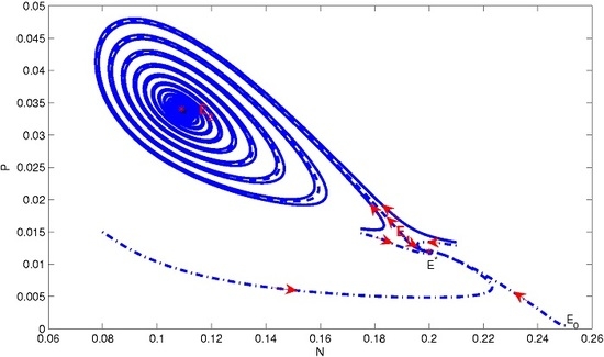
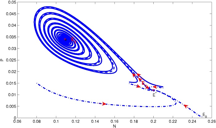
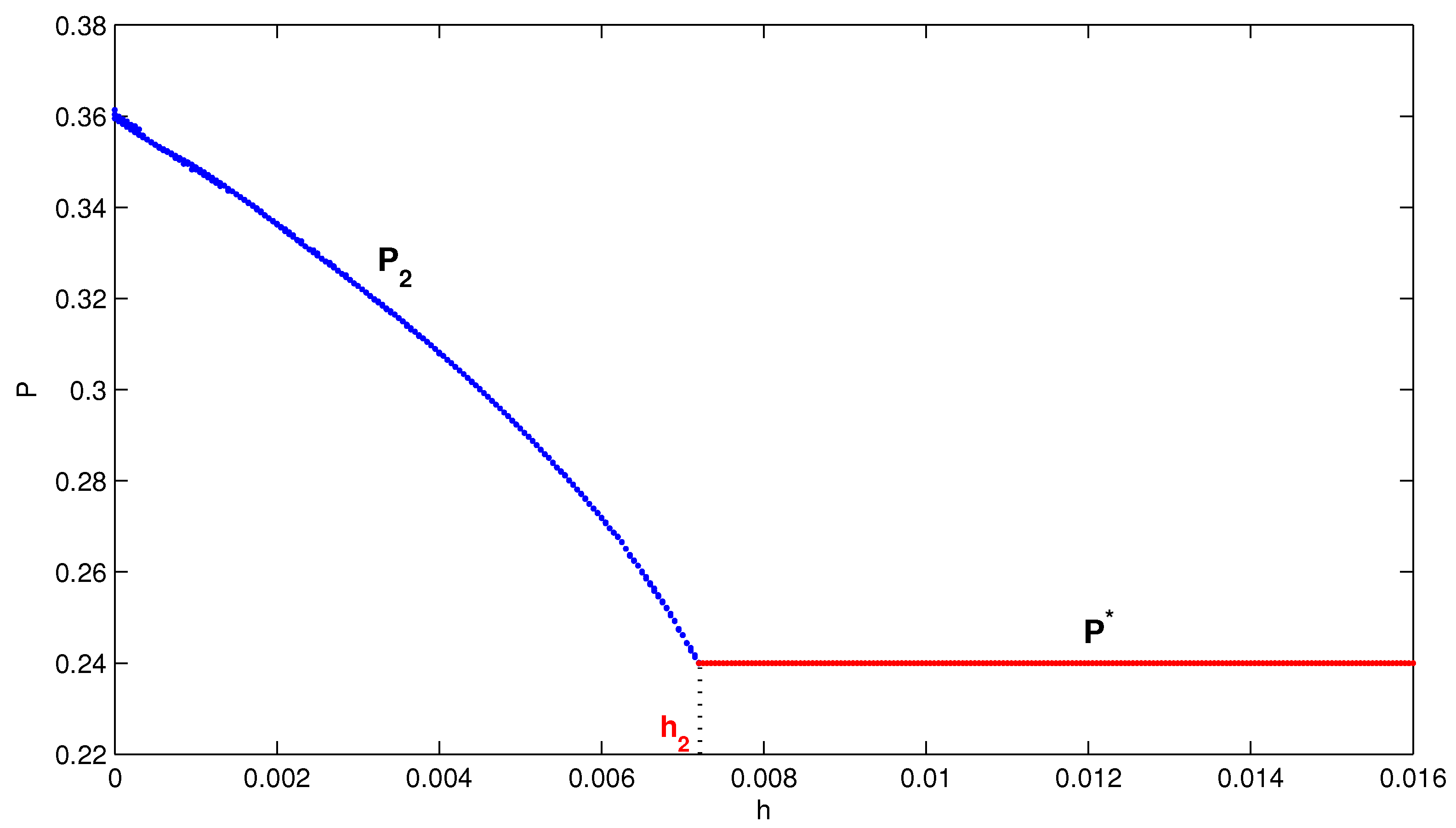
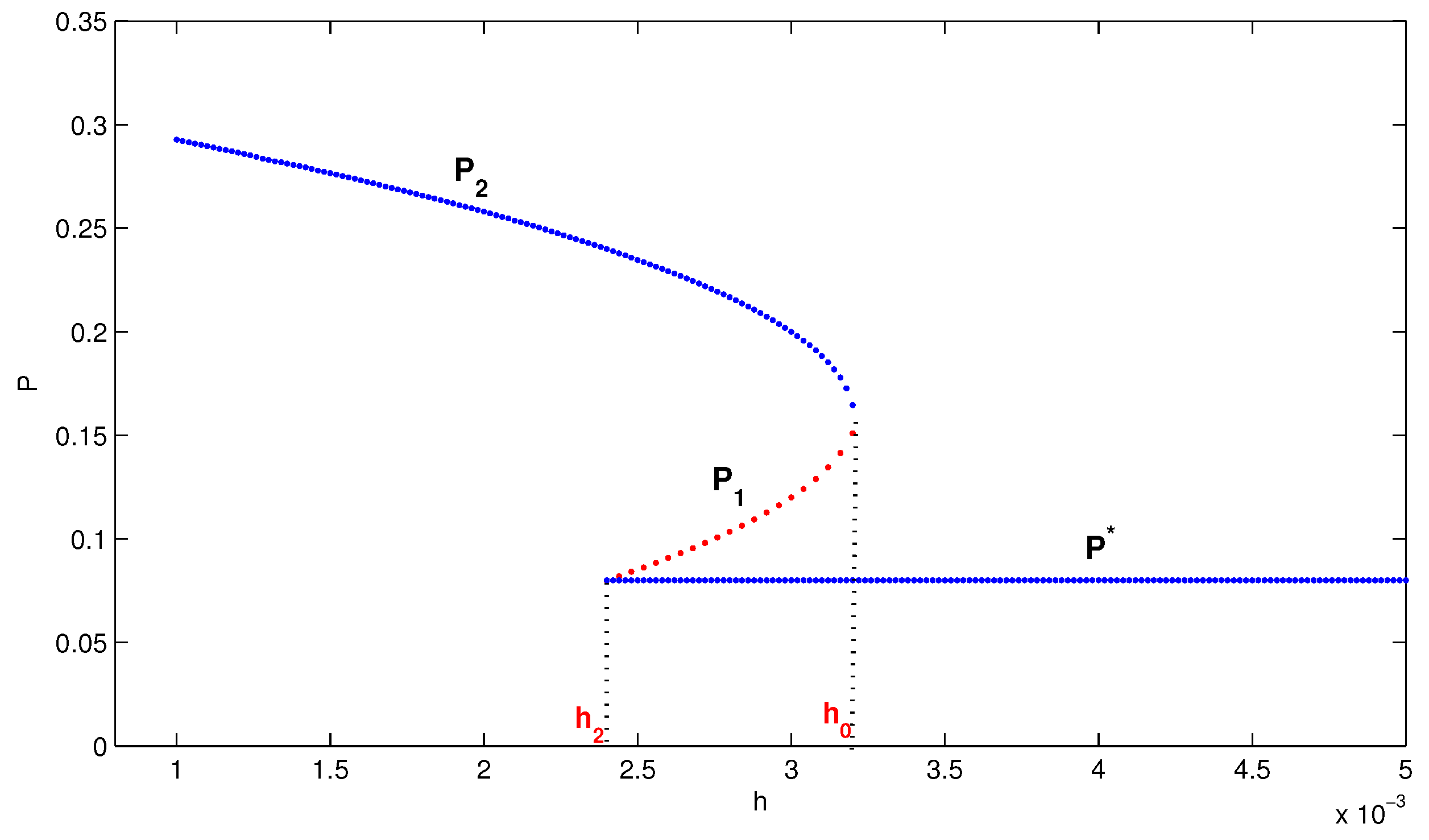
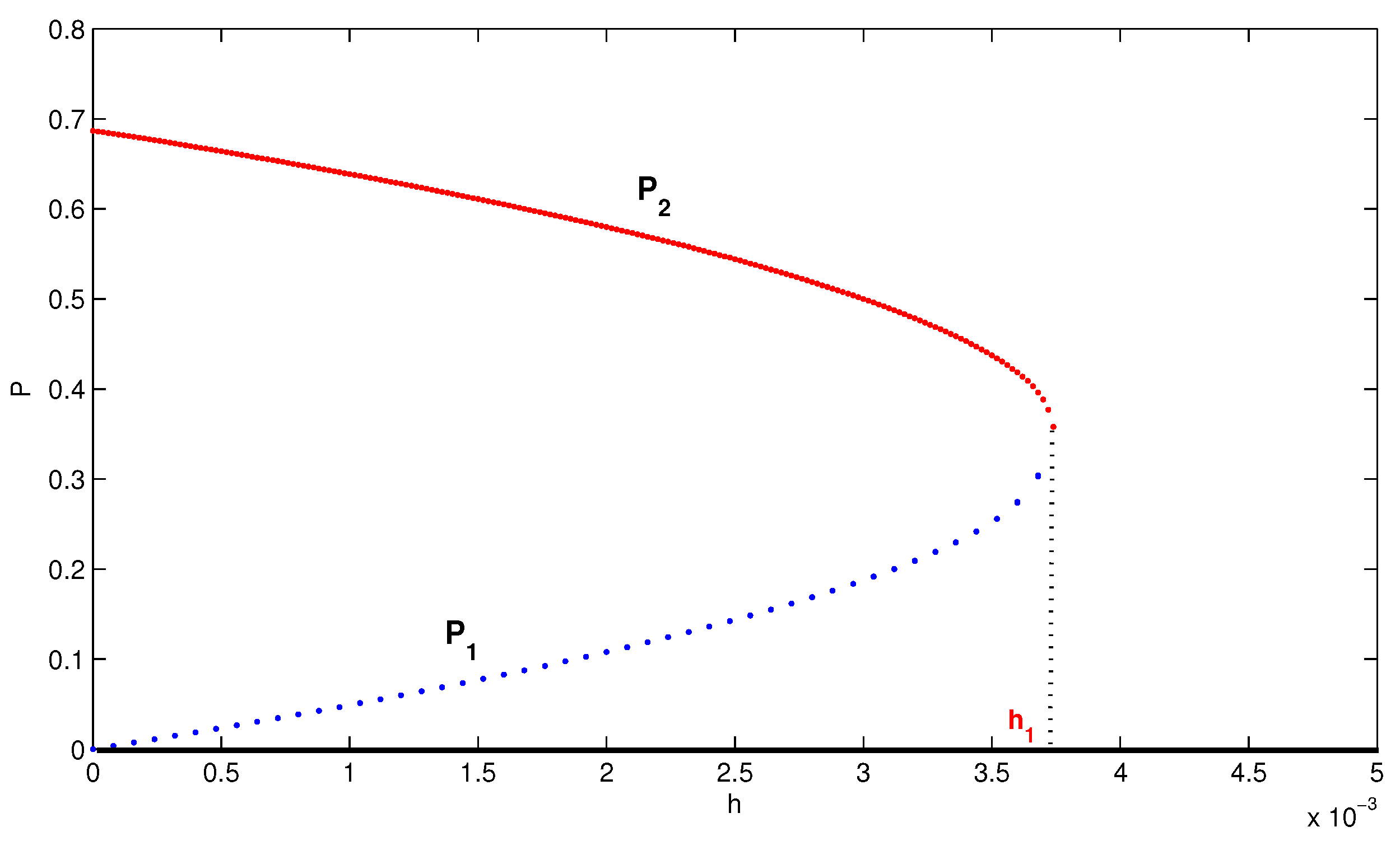
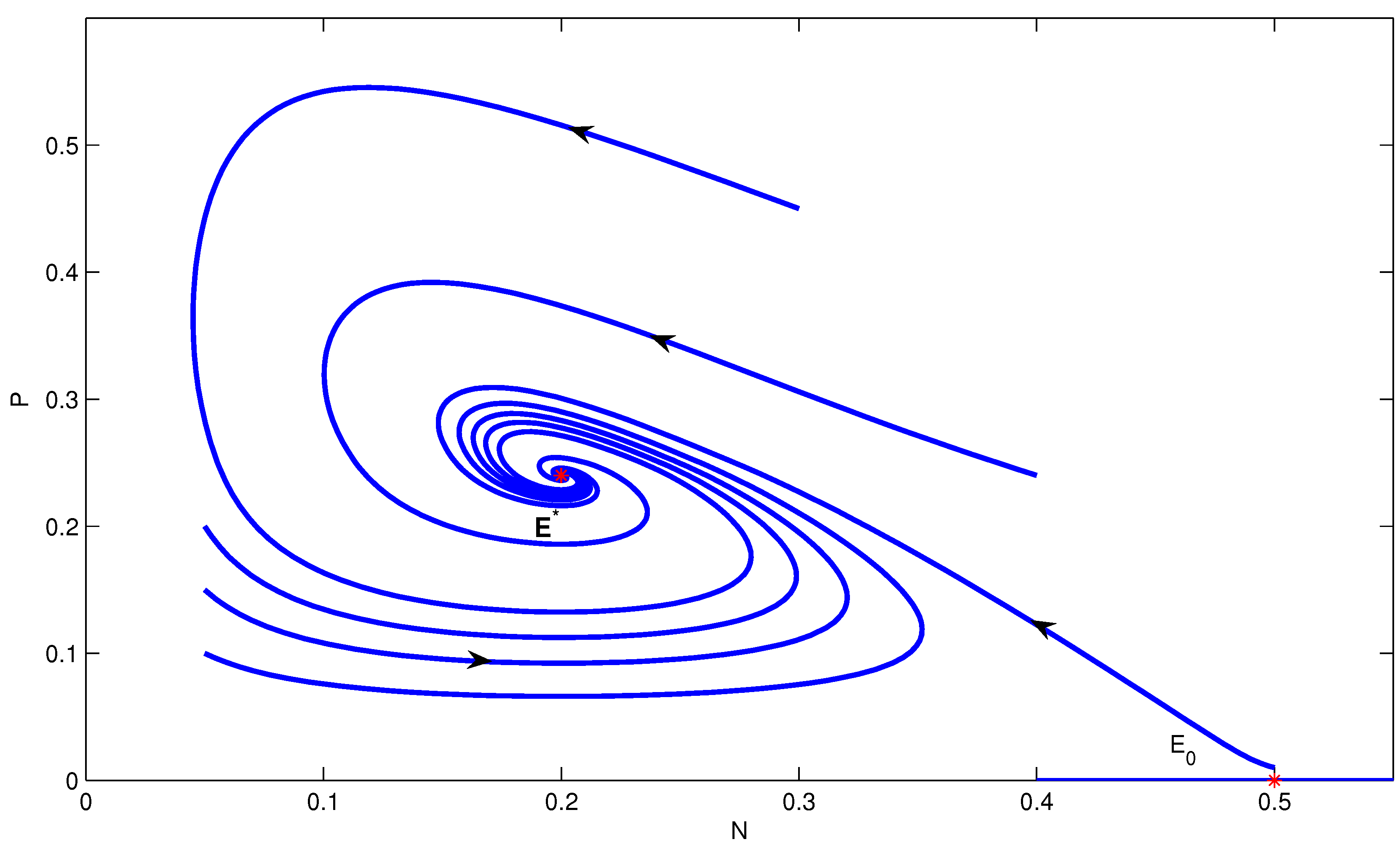
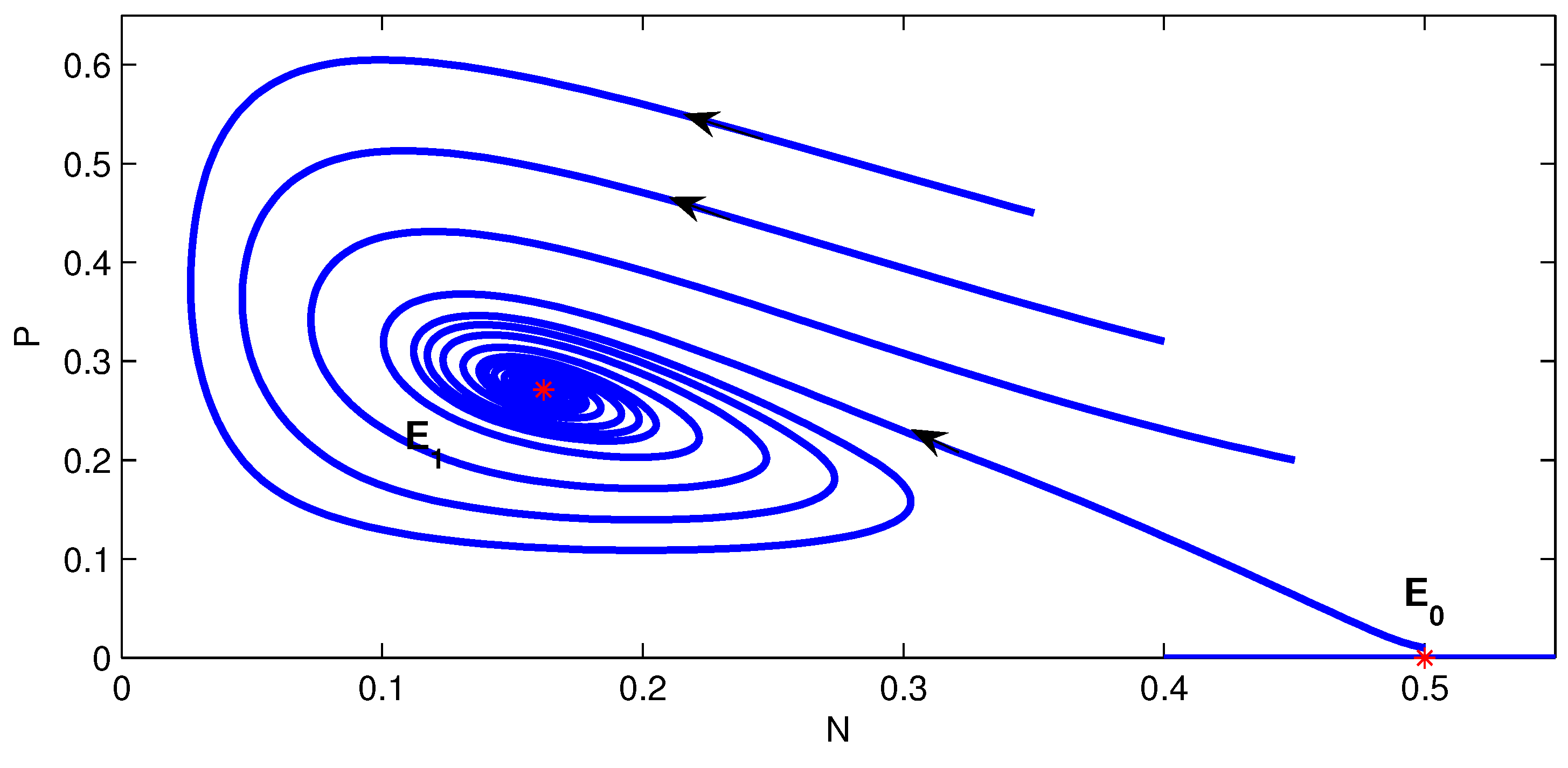
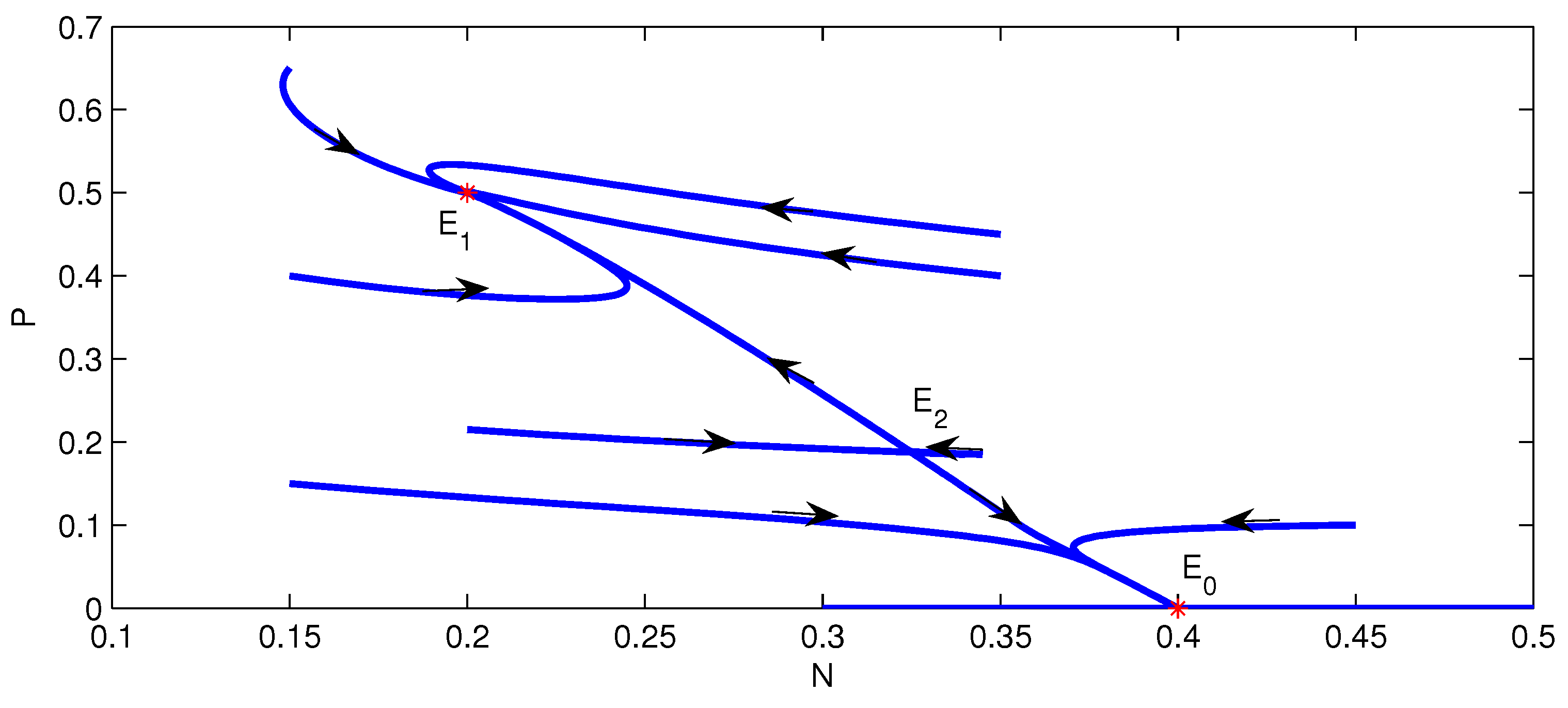
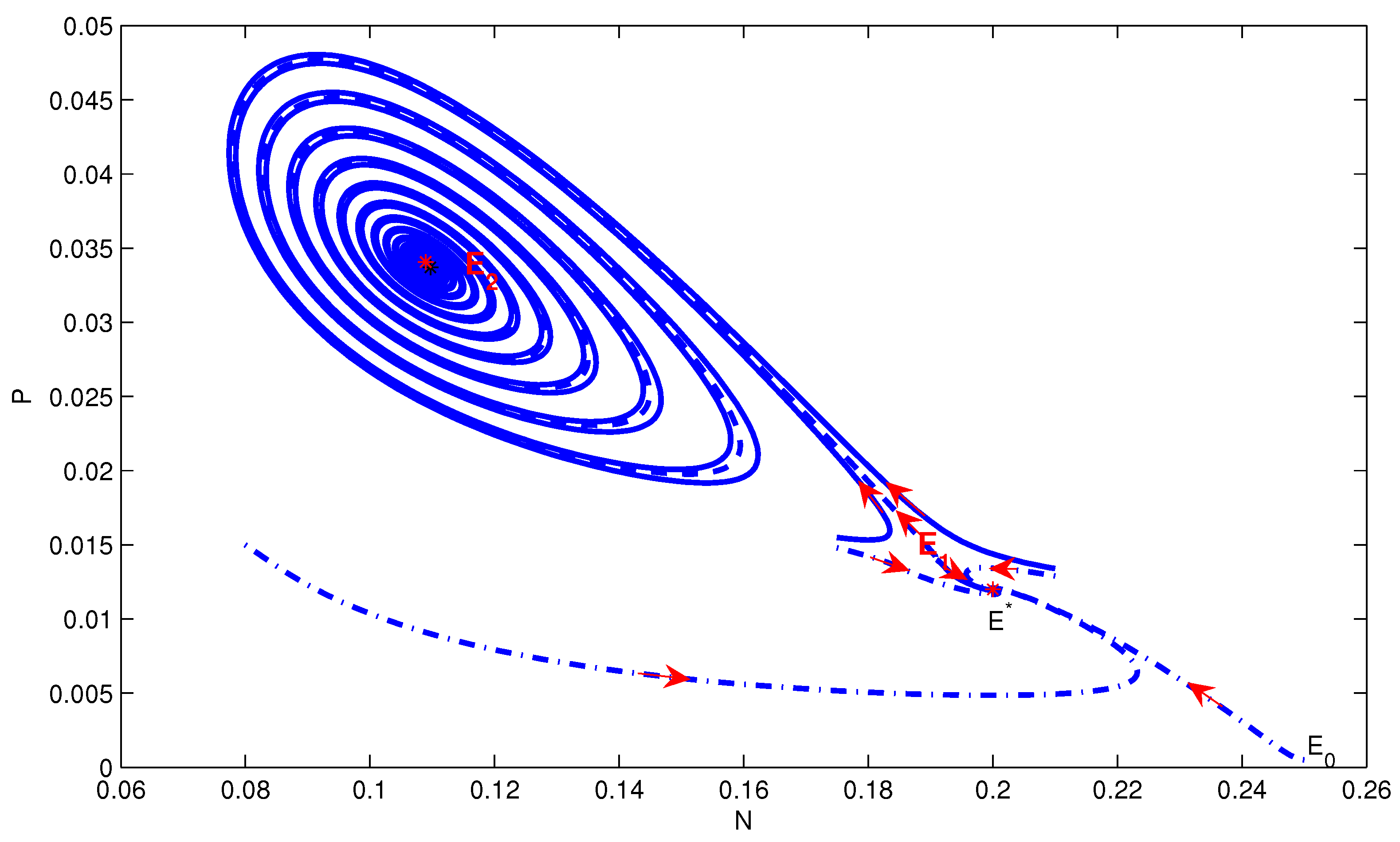
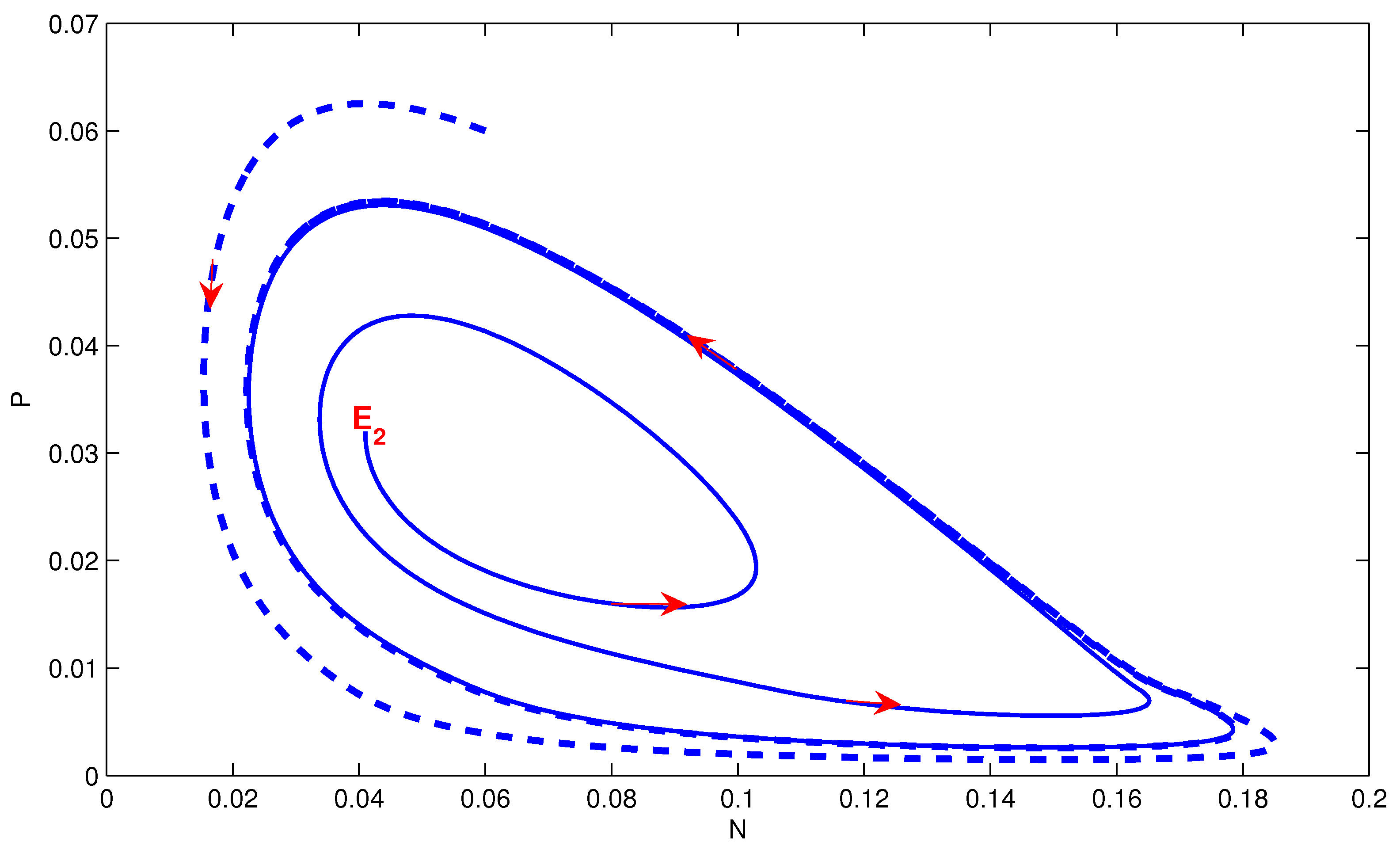
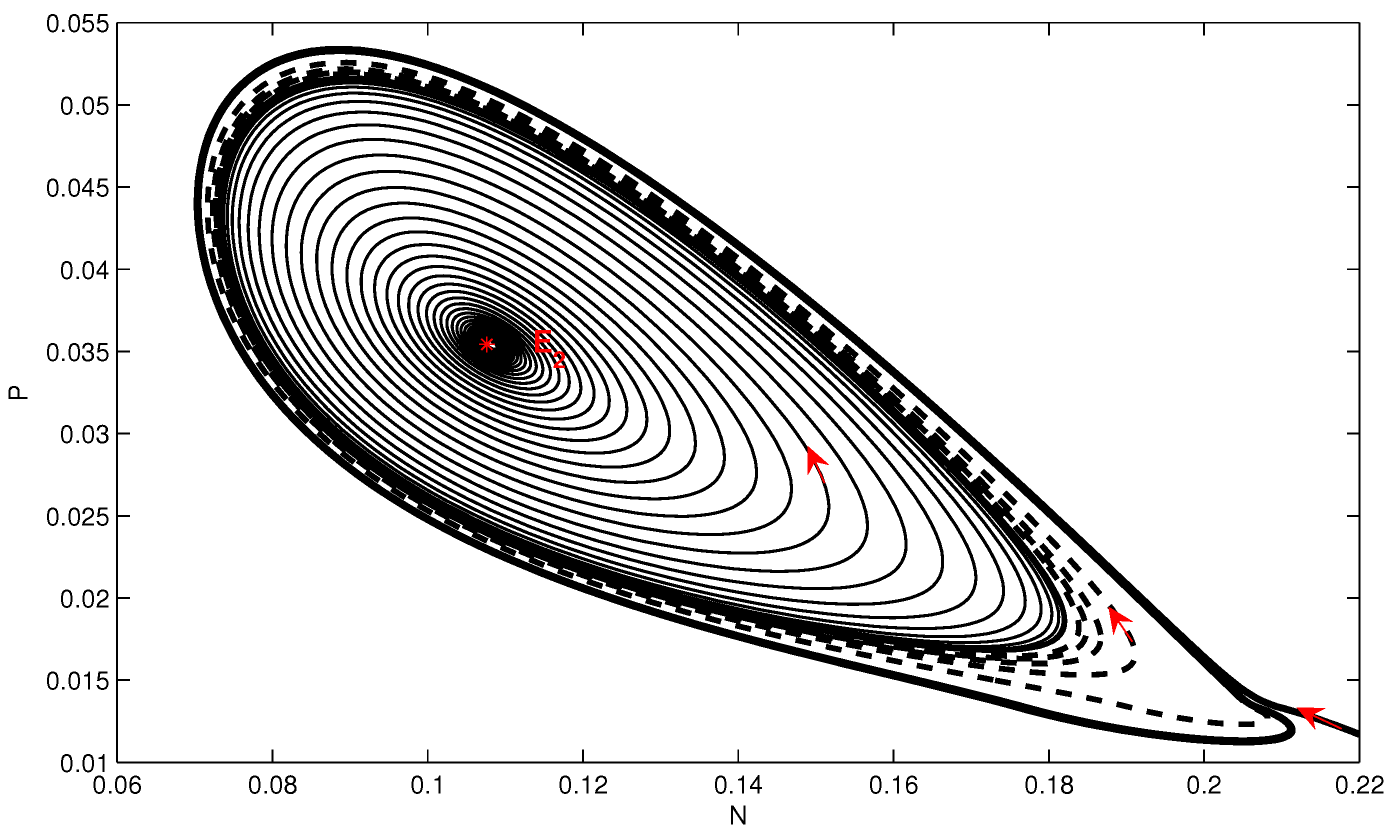
4. Numerical Simulation

In this section, we present numerical examples for system Equation (3).

Example 4.1. 

(Example 3.1. continued) The parameters values $r,K,a,c,d$ and m are the same as in Example 3.1. We obtain $\widehat{n}>1$, $h_1=0.0081$, and $h_2=0.0072$. A forward bifurcation diagram is given in Figure 1.

Selecting $P_0=0.25$, we get $h=0.0075>h_2$. The equilibrium $E^{*}(0.2,0.24)$ exists, but $E_1$ and $E_2$ do not exist (Theorem 2 $b)$). Its phase portrait is given in Figure 4, which shows that the unique positive equilibrium $E^{*}$ is globally asymptotically stable.

Figure 4. The phase portrait of model Equation (3) when $E^{*}$ is globally asymptotically stable and $E_0$ is unstable.

If we choose $P_0=0.2$, then $h=0.006<h_2$. Equilibrium $E_1(0.16044,0.27165)$ exists, but $E_2$ and $E^{*}$ do not exist (Theorem 2 $b)$). Its phase portrait is given in Figure 5. The unique positive equilibrium $E_1$ is globally asymptotically stable in D.

Figure 5. The phase portrait of model Equation (3) when $E_1$ is locally asymptotically stable and $E_0$ is unstable.

The equilibrium $E^{*}$ in Figure 4 corresponds to some point on the curve of $P^{*}$ in Figure 1 ($h>h_2$), and the equilibrium $E_1$ in Figure 5 corresponds to some point on the curve of $P_1$ in Figure 1 ($h<h_2$).

Example 4.2. 

(Example 3.2. continued) Choosing the same parameters values as in Example 3.2, we have $h_1=0.00378$ and $\widehat{P}=0.34367$. A backward bifurcation diagram is given in Figure 2.

If we choose $P_0=0.1$, then $P_0<\widehat{P}$. Equilibria $E_1(0.2,0.5)$ and $E_2(0.325,0.1875)$ exist, but equilibrium $E^{*}$ does not exist. Its phase portrait is illustrated in Figure 6. It shows that equilibria $E_0$ and $E_1$ are asymptotically stable.

Figure 6. The phase portrait of model Equation (3) when $E_0$ and $E_1$ are locally asymptotically stable and $E_2$ is unstable.

The equilibria $E_1$ and $E_2$ in Figure 6 correspond to some points on the curves of $P_1$ and $P_2$ , respectively, in Figure 2 ($h<h_1$).

Example 4.3 (I). 

(Example 3.3. continued) We identically select parameter values as in Example 3.3, and set $P_0=0.1$. Thus we have $\widehat{n}>1$, $h_1=0.0032$, $h_2=0.0024$, $\widehat{P}=0.16$, and $h=0.003$. The above parameter values satisfy conditions $a)$ and $c)$ in Theorem 2, and condition $a)$ in Theorem 6.

Obviously, equilibria $E_0(0.25,0)$, $E^{*}(0.2,0.08)$, $E_1(0.125,0.2)$, and $E_2(0.175,0.12)$ all exist. The phase portrait of model Equation (3) is shown in Figure 7. Equilibria $E^{*}$ and $E_1$ are asymptotically stable, and $E_0$ and $E_2$ are unstable. So model Equation (3) has bistable positive equilibria $E^{*}$ and $E_1$.

Figure 7. The phase portrait of model Equation (3) with bistable positive equilibria $E^{*}$ and $E_1$, and unstable equilibria $E_0$ and $E_2$.

It follows from Figure 7 that the stable region ${\mathsf{\Gamma }}^s$ of the saddle point $E_2$ divides the positive invariant set into two regions. The attractive basin for the stable equilibrium $E_1$ is the region above ${\mathsf{\Gamma }}^s$ and the region below ${\mathsf{\Gamma }}^s$ is the basin of attraction for the stable equilibrium $E^{*}$.

The equilibria $E_1$ and $E_2$ in Figure 7 correspond to some points on the curves of $P_1$ and $P_2$, respectively, and $E^{*}$ corresponds to some point on the curve of $P^{*}$ in Figure 3 ($h_2<h<h_1$).

Example 4.3 (II). 

We set parameter values $r=0.03,K=0.25,a=0.5,c=0.4,d=0.01,m=0.03$, and $P_0=0.0133$. Thus we have $\widehat{n}=1.25$, $u{h}_1=0.00048$, $h_2=0.00036$, $\widehat{P}=0.024$, and $h=0.000399$. These parameter values satisfy conditions $a)$ and $c)$ in Theorem 2 and the condition $c)$ in Theorem 6. Thus, equilibria $E_0(0.25,0)$, $E^{*}(0.2,0.012)$, $E_1(0.1092,0.0338)$, and $E_2(0.1908,0.0142)$ all exist. The phase portrait of model Equation (3) is shown in Figure 8. Equilibria $E^{*}$ and $E_1$ are stable, and $E_0$ and $E_2$ are unstable. So model Equation (3) has bistable positive equilibria $E^{*}$ and $E_1$.

Figure 8. The phase portrait of model Equation (3) with positive stable equilibria $E^{*}$ and $E_1$, and unstable equilibria $E_0$ and $E_2$.

The model with the parameter values in Example 4.3 (II) has a similar bifurcation diagram as that in Example 4.3 (I), and the stability of equilibria in Figure 8 is identical with that in Figure 7.

Example 4.4 (I). 

We select $r=0.004,K=0.2,a=0.1,c=0.4,d=0.001$ and $m=0.005$. Then $\widehat{n}=1.333$, $h_1=6.125*{10}^{-5}$, $\widehat{P}=1.75*{10}^{-2}$, and $h_2=5*{10}^{-5}$.

Choosing $P_0=0.008$, we have $h=2*{10}^{-5}$. Thus, $h<h_2<h_1$, $P_0<\widehat{P}$, $caK>r$, $h>h_3$, and $\eta <0$. Equilibrium $E_1(0.04069,0.03186)$ exists but is unstable, and $E^{*}$ and $E_2$ do not exist. The parameter values satisfy the conditions of Theorem 7. Its phase portrait is given in Figure 9, which shows that model Equation (3) has a stable limit cycle which encircles $E_1$.

Figure 9. A stable limit cycle of model Equation (3) encircling the unstable equilibrium $E_1$.

Example 4.4 (II). 

Set $r=0.03,K=0.264,a=0.5,c=0.4,d=0.01$, and $m=0.031$. We obtain $\widehat{n}=1.2878$, $h_1=5.2041*{10}^{-4}$, $\widehat{P}=2.4318*{10}^{-2}$, and $h_2=4.1568*{10}^{-4}$.

Choosing $P_0=0.0133$, we obtain $h=4.123*{10}^{-4}$. The parameter values satisfy Theorem 2 $\left(b\right)$ and Theorem 6 $\left(c\right)$, but do not satisfy Theorem 2 $\left(a\right)$. Thus, equilibria $E^{*}$ and $E_2$ do not exist and $E_1(0.1082,0.0354)$ exists. The phase portrait of model Equation (3) is shown in Figure 10. In Figure 10, equilibrium $E_1$ is stable and two periodic orbits encircle $E_1$. We can see that the outside periodic orbit is stable. However, the inside periodic orbit is unstable. A trajectory (the dotted line) between the outside and inside periodic orbits ultimately tends to the outside periodic orbit, but a trajectory (the thin black line) starting from within the unstable periodic orbit finally tends to equilibrium $E_1$. So the initial state is important for ultimate trends of trajectories.

Figure 10. The phase portrait of model Equation (3) when $E_1$ is stable.

5. Conclusions

In this paper, we proposed and studied a new predator-prey model with non-smooth switched harvest on the predator. If the density of the predator is below a switched value, the harvest has a linear harvesting rate. Otherwise, the harvesting rate is constant. Our model exhibits new dynamical features compared to those with a linear harvesting rate or a constant harvesting rate.

According to the Kolmogorov Theorem [38], under certain assumptions, the model with a linear predator harvesting rate has either a stable equilibrium or a stable limit cycle, whereas the model with a constant harvesting rate on the predator has richer dynamics [16,23,16]. For example, for a class of predator-prey systems, Brauer and Soudack [23,23] obtained different types of dynamics for which the harvesting was in prey or a predator; Xiao and Jennings [16] further studied a ratio-dependent predator-prey model with a constant harvest on prey. They proved that the model could exhibit complicated bifurcation phenomena, including the Bogdanov-Takens bifurcation of cusp type, the heteroclinic bifurcation, or a separatrix connecting a saddle-node and a saddle bifurcation.

For the model studied in this paper, we showed that (see Theorem 2 and Corollary 1) a backward bifurcation from the predator-prey coexistence equilibrium may occur, which shows that reducing the net reproductive number of the predator to less than unity is not enough to eradicate the predator. On the other hand, when the net reproductive number of the predator is greater than unity, we showed that the predator always coexists with the prey permanently (Theorem 3), and the model may exhibit the following dynamics: (i) a unique globally asymptotically stable coexistence equilibrium; (ii) the coexistence of positive saddle equilibria connecting with either a locally asymptotically stable positive equilibrium (biostable) or a limit cycle; (iii) two stable positive equilibria coexisting with a saddle point. By numerical examples, we also showed that the model could exhibit more new dynamical features: (a) a limit cycle encircling a unique positive equilibrium (see Figure 9); (b) two cycles surround an identical positive equilibrium, with one stable and one unstable (see Figure 10).

We would like to point out that we have assumed the simple functional response of the bilinear type in our current model Equation (3). We may also consider other types of functional responses. The dynamics may be richer and more complex. Further investigations are planned in our future studies.

References

- Murdoch, W.W.; Briggs, C.J.; Nisbet, R.M. Consumer-Resource Dynamics; Princeton University Press: Princeton, NJ, USA, 2003. [Google Scholar]
- Seo, G.; DeAngelis, D.L. A predator-prey model with a Holling type I functional response including a predator mutual interference. J. Nonlinear Sci. 2011, 21, 811–833. [Google Scholar] [CrossRef]
- Turchin, P. Complex Population Dynamics: A Theoretical/empirical Synthesis; Princeton University Press: Princeton, NJ, USA, 2003. [Google Scholar]
- Gutierrez, A.P. Applied Population Ecology: A Supply-Demand Approach; John Wiley and Sons: New York, NY, USA, 1996. [Google Scholar]
- Seo, G.; Kot, M. A comparison of two predator-prey models with Hollingąŕs type I functional response. Math. Biosci. 2008, 212, 161–179. [Google Scholar] [CrossRef] [PubMed]
- Cushing, J.M.; Zou, Y. The net reproductive value and stability in matrix population models. Nat. Resour. Model. 1994, 8, 297–333. [Google Scholar]
- Cushing, J.M. An Introduction to Structured Population Dynamics; SIAM: Philadelphia, PA, USA, 1998. [Google Scholar]
- Kar, T.K. Stability analysis of a prey-predator model incorporating a prey refuge. Commun. Nonlinear Sci. Numer. Simul. 2005, 10, 681–691. [Google Scholar] [CrossRef]
- Chakraborty, K.; Haldar, S.; Kar, T.K. Global stability and bifurcation analysis of a delay induced prey-predator system with stage structure. Nonlinear Dyn. 2013, 73, 1307–1325. [Google Scholar] [CrossRef]
- Liu, S.Q.; Beretta, E. A stage-structured predator-prey model of Beddington-Deangelis type. SIAM J. Appl. Math. 2006, 66, 1101–1129. [Google Scholar] [CrossRef]
- Qu, Y.; Wei, J.J. Bifurcation analysis in a time-delay model for preyĺCpredator growth with stage-structure. Nonlinear Dyn. 2007, 49, 285–294. [Google Scholar] [CrossRef]
- Zhang, X.A.; Chen, L.S.; Neumann, A.U. The stage-structured predator-prey model and optimal harvesting policy. Math. Biosci. 2000, 168, 201–210. [Google Scholar] [CrossRef]
- Zhang, Y.; Zhang, Q.L. Dynamic behavior in a delayed stage-structured population model with stochastic fluctuation and harvesting. Nonlinear Dyn. 2011, 66, 231–245. [Google Scholar] [CrossRef]
- Lai, X.H.; Liu, S.Q.; Lin, R.Z. Rich dynamical behaviours for predator-prey model with weak Allee effect. Appl. Anal. 2010, 89, 1271–1292. [Google Scholar] [CrossRef]
- Lin, R.Z.; Liu, S.Q.; Lai, X.H. Bifurcations of a predator-prey system with weak Allee effects. J. Korean Math. Soc. 2013, 50, 695–713. [Google Scholar] [CrossRef]
- Xiao, D.M.; Jennings, L.S. Bifurcations of a ratio-dependent predator-prey system with constant rate harvesting. SIAM J. Appl. Math. 2005, 65, 737–753. [Google Scholar] [CrossRef]
- Xiao, D.M.; Li, W.X.; Han, M.A. Dynamics in a ratio-dependent predator-prey model with predator harvesting. J. Math. Anal. Appl. 2006, 324, 14–29. [Google Scholar] [CrossRef]
- Zhang, Y.; Zhang, Q.L.; Zhang, X. Dynamical behavior of a class of prey-predator system with impulsive state feedback control and Beddington-DeAngelis functional response. Nonlinear Dyn. 2012, 70, 1511–1522. [Google Scholar] [CrossRef]
- Gao, Y.; Liu, S.Q. Global stability for a predator-prey model with dispersal among patches. Abstr. Appl. Anal. 2014, 2014, 176493. [Google Scholar] [CrossRef]
- Martin, A.; Ruan, S.G. Predator-prey models with delay and prey harvesting. J. Math. Biol. 2001, 43, 247–267. [Google Scholar] [CrossRef] [PubMed]
- Wei, C.J.; Chen, L.S. Periodic solution and heteroclinic bifurcation in a predatorĺCprey system with Allee effect and impulsive harvesting. Nonlinear Dyn. 2014, 76, 1109–1117. [Google Scholar] [CrossRef]
- Azar, C.; Holmberg, J.; Lindgren, K. Stability analysis of harvesting in a predator-prey model. J. Theor. Biol. 1995, 174, 13–19. [Google Scholar] [CrossRef]
- Brauer, F.; Soudack, A.C. Stability regions and transition phenomena for harvested predator-prey systems. J. Math. Biol. 1979, 7, 319–337. [Google Scholar] [CrossRef]
- Brauer, F.; Soudack, A.C. Stability regions in predator-prey systems with constant-rate prey harvesting. J. Math. Biol. 1979, 8, 55–71. [Google Scholar] [CrossRef]
- Kar, T.K. Selective harvesting in a prey-predator fishery with time delay. Math. Comput. Model. 2003, 38, 449–458. [Google Scholar] [CrossRef]
- Lenzini, P.; Rebaza, J. Nonconstant predator harvesting on ratio-dependent predator-prey models. Appl. Math. Sci. 2010, 4, 791–803. [Google Scholar]
- Negi, K.; Gakkhar, S. Dynamics in a Beddington-DeAngelis prey-predator system with impulsive harvesting. Ecol. Model. 2007, 206, 421–430. [Google Scholar] [CrossRef]
- Xiao, M.; Cao, J.D. Hopf bifurcation and non-hyperbolic equilibrium in a ratio-dependent predator-prey model with linear harvesting rate: Analysis and computation. Math. Comput. Model. 2009, 50, 360–379. [Google Scholar] [CrossRef]
- Beddington, J.R.; Cooke, J.K. Harvesting from a prey-predator complex. Ecol. Model. 1982, 14, 155–177. [Google Scholar] [CrossRef]
- Hu, Z.X.; Ma, W.B.; Ruan, S.G. Analysis of an SIR epidemic model with nonlinear incidence rate and treatment. Math. Biosci. 2012, 238, 12–20. [Google Scholar] [CrossRef] [PubMed]
- Wang, W.D. Backward bifurcation of an epidemic model with treatment. Math. Biosci. 2006, 201, 58–71. [Google Scholar] [CrossRef] [PubMed]
- Zhang, X.; Liu, X.N. Backward bifurcation and global dynamics of an SIS epidemic model with general incidence rate and treatment. Nonlinear Anal. Real World Appl. 2009, 10, 565–575. [Google Scholar] [CrossRef]
- Cantrell, R.S.; Cosner, C. On the dynamics of predator-prey models with the Beddington—DeAngelis functional response. J. Math. Anal. Appl. 2001, 257, 206–222. [Google Scholar] [CrossRef]
- Lu, Y.; Li, D.; Liu, S.Q. Modeling of hunting strategies of the predators in susceptible and infected prey. Appl. Math. Comput. 2016, 284, 268–285. [Google Scholar] [CrossRef]
- Hale, J.; Waltman, P. Persistence in infinite-dimensional systems. SIAM J. Math. Anal. 1989, 20, 388–395. [Google Scholar] [CrossRef]
- McCluskey, C. Lyapunov Functions for Tuberculosis Models with Fast and Slow Progression. Math. Biol. Eng. 2006, 3, 603–614. [Google Scholar] [CrossRef]
- Hale, J.; Lunel, S.V. Introduction to Functional Differential Equations; Springer-Verlag: New York, NY, USA, 1993. [Google Scholar]
- Freedman, H.I. Deterministic Mathematical Models in Population Ecology; Marcel Dekker: New York, NY, USA, 1980. [Google Scholar]
- Cui, J.; Mu, X.; Wan, H. Saturation recovery leads to multiple endemic equilibria and backward bifurcation. J. Theor. Biol. 2008, 254, 275–283. [Google Scholar] [CrossRef] [PubMed]
- Van den Driessche, P.; Watmough, J. Reproduction numbers and sub-threshold endemic equilibria for compartmental models of disease transmission. Math. Biosci. 2002, 180, 29–48. [Google Scholar] [CrossRef]
- McQuaid, C.F.; Britton, N.F. Trophic structure, stability, and parasite persistence threshold in food webs. Bull. Math. Biol. 2013, 75, 2196–2207. [Google Scholar] [CrossRef] [PubMed]
- Zhang, X.; Liu, X.N. Backward bifurcation of an epidemic model with saturated treatment function. J. Math. Anal. Appl. 2008, 348, 433–443. [Google Scholar] [CrossRef]
- Zhou, L.H.; Fan, M. Dynamics of an SIR epidemic model with limited medical resources revisited. Nonlinear Anal. Real World Appl. 2012, 13, 312–324. [Google Scholar] [CrossRef]
© 2016 by the authors; licensee MDPI, Basel, Switzerland. This article is an open access article distributed under the terms and conditions of the Creative Commons Attribution (CC-BY) license (http://creativecommons.org/licenses/by/4.0/).