Article

Tracking a Driver’s Face against Extreme Head Poses and Inference of Drowsiness Using a Hidden Markov Model

Department of Computer Engineering, Sejong University, Seoul 143-747, Korea
*
Author to whom correspondence should be addressed.
Appl. Sci. 2016, 6(5), 137; https://doi.org/10.3390/app6050137
Submission received: 9 March 2016 / Revised: 6 April 2016 / Accepted: 27 April 2016 / Published: 7 May 2016

Abstract

:
This study presents a new method to track driver’s facial states, such as head pose and eye-blinking in the real-time basis. Since a driver in the natural driving condition moves his head in diverse ways and his face is often occluded by his hand or the wheel, it should be a great challenge for the standard face models. Among many, Active Appearance Model (AAM), and Active Shape Model (ASM) are two favored face models. We have extended Discriminative Bayesian ASM by incorporating the extreme pose cases, called it Pose Extended—Active Shape model (PE-ASM). Two face databases (DB) are used for the comparison purpose: one is the Boston University face DB and the other is our custom-made driving DB. Our evaluation indicates that PE-ASM outperforms ASM and AAM in terms of the face fitting against extreme poses. Using this model, we can estimate the driver’s head pose, as well as eye-blinking, by adding respective processes. Two HMMs are trained to model temporal behaviors of these two facial features, and consequently the system can make inference by enumerating these HMM states whether the driver is drowsy or not. Result suggests that it can be used as a driver drowsiness detector in the commercial car where the visual conditions are very diverse and often tough to deal with.

Graphical Abstract

1. Introduction

According to National Highway Traffic Safety Administration (NHTSA), drowsy driving causes more than 100,000 crashes a year [1]. Drowsiness, in general, refers to a driver in a trance state while driving. The most common symptom of drowsiness includes excessive yawning and frequent eye-blinking due to difficulty of keeping one’s eyes open. Symptoms also include reduced steering wheel operation and frequent head-nodding. The European Transport Safety Council (ETSC) (Brussels, Belgium)indicates that increment of the above-mentioned symptoms means that the driver is in drowsiness [2].
Automotive manufacturers are conducting diverse researches focusing on anti-drowsiness safety devices to prevent drowsy driving. Typical driver drowsiness detection methods includes learning driving patterns (operation of steering, speed acceleration/reduction, gear operation) or measuring brainwave (EEG), heartbeat, and body temperature to recognize and prevent the drowsy driving. Among many approaches, the non-contact sensor such as camera is often favored in detecting yawning, or tracking the head movement and eye-blink of the driver. Indeed, NHTSA and ETSC manuals suggest that detection and tracking of driver’s eye-blinking is the most reliable way in determining the consciousness level of the driver.
Given that camera sensors are now cheap and can be combined with the infra-red LEDs for the night driving environment, it appears that observing visual appearance of the face in determining the mental state of the driver becomes a main trend. In doing so, it is essential to have a good face model by which we can track the driver’s the face and facial features reliably against head pose variation, illumination change, and self-occlusion occurring sporadically during the natural driving situation.
One of the popular face models was initially proposed by Tim Cootes, the so called Point Distribution Model (PDM) [3,4]. There are two variations of it: one is Active Appearance Model (AAM) and the other Active Shape Model (ASM). AAM consists of appearance and shape parameters. Two versions have been developed depending on the way of dealing with these parameters: the initial model is the combined AAM [5] and the other the independent AAM [6].
AAM has been very successful in face recognition, face tracking, and facial expression recognition areas. Yet its performance varies depending on the training method and the amount of data. Moreover, it is slow since it requires a lot of computation during the fitting, and it suffers from illumination variation and occlusion. Although an improvement regarding to the illumination variation, occurring frequently in the mobile environment, has been reported by adopting a Difference of Gaussian (DoG) filter [7], the speed and occlusion problems are yet to be solved.
ASM has been developed to align the shape of the face and it has a certain advantage in terms of speed simply because it has only one set of parameters (i.e., the shape). However, the whole alignment process can be degraded by an error on any landmark drawn on the tracking face. To handle such problem, the Constrained Local Model (CLM) has been proposed [
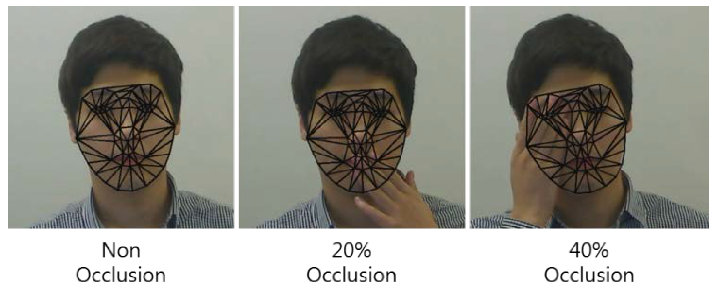
8], where each shape landmark detects the local feature and then carries out tracking independently. Therefore, the performance critically depends on local feature detection and tracking, rather than any training method and data. In CLM, the shape generated at each landmark has the highest probability. Since each landmark is processed independently, it allows parallel processing. In the conventional AAM and ASM, the previous error often affects the present state. However, any error occurring in a local feature detector has minimal impact to the overall performance since each landmark behaves independently. Due to such reasons, ASM based on CLM shows robustness against occlusion.
In this study, we will use an updated version of ASM, called it Discriminative Bayesian—Active Shape Model (DB-ASM) [9,10] as a base model. Yet, even this model cannot deal with the extremes head pose cases well, for instance, when the driver looks at the side mirrors. Compared to the standard face model that contains average shape landmarks during the training stage, the extended version includes six more average shape landmarks to cover the extreme poses, such as look up, look down, rotated left, rotated right, look left, and look right, respectively, so called Pose Extended ASM (PE-ASM). Note that each head pose model has been independently trained. The POSIT (Pose from Orthography and Scaling with Iterations) algorithm is employed to estimate the present head pose of the given face [11]. When the driver’s head pose crosses a certain threshold along a given direction, PE-ASM detects that and assigns the corresponding extreme average shape. Thus, the newly assigned model can track the head even when the head is in an extreme pose.
In monitoring driver’s drowsiness, many previous studies have actually adopted the geometrical approach rather than the statistical one, presumably because the latter is heavy or is not reliable at that time. For instance, Ji and Yang [12] were able to build a real-time system using several visual cues, such as gaze, face pose, eyelid closure, approached by the geometrical perspective. Recently, Mbouna et al. [13] proposed a driver alertness monitoring system where a 3D graphical head model is combined with a POSIT algorithm in estimating driver’s head pose, and an eye index is designed in determining eye opening during driving.
Markov models are stochastic models used in analysis of time varying signals. Since HMM has been a powerful tool in modelling continuous signals, such as natural language processing, speech understanding, and computer vision [14]. Modified versions of HMMs have also been proposed for computer vision, such as coupled or multi-dimensional models. It is shown that driver’s eye-movements can be modelled using an HMM [15]. The driver’s behavior has also been modelled using HMM [16]. In the present study, we have used a Markov chain framework whereby the driver’s eye-blinking and head nodding are separately modelled based upon their visual features, and then the system makes a decision by combining those behavioral states of whether the driver is drowsy or not, according to a certain criteria.

2. Discriminative Bayesian—Active Shape Model (DB-ASM)

DB-ASM is a face model that is based on Active Shape Model (ASM) [9]. One of its evolutions is the Constrained Local Model (CLM) in which a global face model is created by combining the local feature detections [8,10]. The global model is composed of a Point Distribution Model (PDM), which is acquired by updating the several parameters at each landmark drawn on the face image. In the present study, DB-ASM utilizes the Minimum Output Sum of Squared Error (MOSSE) filter [17] for the local feature detection because it is known to be fast and reliable. Then, the shape parameters use a Maximum A Posteriori (MAP) update.

2.1. Point Distribution Model

Point Distribution Model (PDM) is used to learn about the face shapes, built by landmark points drawn by hand, using the Principal Component Analysis (PCA) technique. Before this stage, the scale, rotation, and translation were aligned in data by using Procrustes Analysis. The learned average data, and eigen value and eigenvector were statistically combined to complete a model to transform the shape. Equation (1) represents a PDM:
s = S ( s 0 + Φ b s ,   q )
where s 0 = ( x 1 0 , y 1 0 , , x v 0 , x v 0 ) T is the mean shape, Φ is the shape subspace matrix holding n eigenvectors, b s is a vector of shape parameters. S(., q) represents a similarity transformation function of the q = [ s , θ , t x , t y , ] t pose parameters (s, θ , t x , t y are the scale, rotation, and translations with respect to the base mesh s 0 , respectively).

2.2. Feature Detector

As mentioned above, the local feature detector of the present DB-ASM is a MOSSE filter. It is known that it is very fast and robust against rotation and partial occlusion. Equation (2) represents the MOSSE filter.
G = F H *
Since the input image is given as f; filter as h; 2D Gaussian Map as g in the Equation (2), each variable is to produce F, H, G, respectively, through 2D Fourier transform. Here, F is acquired by convoluting an input image using the 2D Fast Fourier Transform (FFT). ʘ refers to the element-wise multiplication, whereas * refers to complex conjugate. The filter in Equation (2) can be derived by using Equation (3) on the local feature image at each location.
H * = j = 1 N G j F j * j = 1 N F j F j *
In Equation (3), each image and Gaussian map are to be treated with FFT and then an element-wise convolution to obtain the cumulative data. The cumulative data is to be divided to obtain the filter H * . The created filter H and input image I are to be treated in the element-wise way and Equation (4) is used to calculate a response map (or correlation map).
D i MOSSE ( I ( y i ) ) =   F 1 { F { I ( y i ) } H i * }
The response map calculated by Equation (4) is to predict the weighted peak with likelihood. Then, an isotropic Gaussian is be obtained through this likelihood. Equation (5) gives the isotropic Gaussian of y i W P .
y i W P in Equation (5) refers to a location having the highest correlation in the response map as shown in Figure 1, whereas y i W P refers to a Gaussian covariance matrix in y i W P and the response map.
y i W P = max z Ω ( p i ( z i ) ) ,   w p y i = diag ( p i ( y i W P ) 1 )
where p i ( ) = R e s p o n s e   M a p .
Figure 1 illustrates the visual appearance of the PDM, the MOSSE filter and the response maps, respectively, at five sampled landmarks among 56 on the given face.

2.3. Shape Update

y i W P and y i W P   obtained in above section are used to update the current shape parameter and to perform a shape fitting. The equation to obtain the prior of shape parameter in Bayesian distribution is shown in Equation (6) as below.
p i ( p k | p k 1 ) N ( b k | μ b   , p   )
The calculated prior shape parameter y i W P , as well as y i W P , are used in updating process. The following Equations (7)–(9) present the updating process.
K =   P k 1 Φ T ( Φ P k 1 Φ T + Σ y )
μ k F = A μ k 1 F + K ( y Φ A μ k 1 F )
Σ k F = ( I n K Φ ) P k 1
A = n dimensional identity matrix, P k = covariance of shape parameter.
Using these equations, the shape parameter and pose parameter can be updated concurrently. The updates are repeated 10 times. When the difference between two shape parameters reaches to a threshold, it ceases the updating process.

3. Detecting a Drowsy Driver

3.1. Head Pose Estimation by the POSIT Algorithm

In this study, the POSIT algorithm is used in estimating the head pose of the driver [11]. Head rotation is calculated by using the initialized standard 3D coordinate and current 2D shape coordinate. It calculates rotation and translation based on the correlation between points on the 2D coordinate space and corresponding points in the 3D coordinate space. Equation (10) is the formula for the POSIT algorithm.
s [ u v 1 ] = [ f x 0 c x 0 f y c y 0 0 1 ] [ r 11 r 12 r 13 r 21 r 22 r 23 r 31 r 32 r 33   t 1 t 2 t 3 ] [ X Y Z 1 ]
Here, (X, Y, Z) represents the coordinate of 3D and ( u , v ) that of 2D, which is obtained based on projection. The camera matrix has intrinsic parameters, which are the center point of image, ( c x , c y ), scale factor ( s ), and focal length between pixels ( f x , f y ), respectively. The rotation matrix and translation matrix [ R | t ] are extrinsic parameters that have r i j and t i j , respectively. The POSIT algorithm estimates the rotation matrix and translation matrix in 3D space.
To use the POSIT algorithm in estimating head pose, a 3D face model is built using FaceGen Modeler 3.0, where the size of 3D face model is average and the coordinate of this 3D space is identical with that of the facial feature. The coordinates of generated 3D facial features are used for input to POSIT.

3.2. Pose Extended-Active Shape Model

In general, it is known that the head pose of a driver changes continuously since one drives a car while watching the side mirrors and rear mirror in turn. In this study, the range of head movement occurred while driving is utilized to determine whether the driver is drowsy or not. In particular, the change of head pose is significant when the driver is looking at the side-mirror to the right rather than the side-mirror to the left. The change of the driver’s head pose and its frequency become an important factor in determining drowsiness of the given driver.
Among many, we can think of two statistical face models, favored in the computer vision community, for the present purpose. One of them is Active Shape Model (ASM) and the other is Active Appearance Model (AAM). Given that the head poses of the normal driver are very diverse and some of them are obviously extreme, the face model certainly needs to deal with such extreme pose cases. However, it is well known that these face models have been effective in estimating the head pose, which is less than about 30°, called the average face shape. Therefore, they cannot deal well in the cases where the head pose is higher than 30°, called the extreme head pose cases.
The reason is that some of extreme shape vectors are lost in carrying out the Principal Component Analysis (PCA) process. Moreover, since the locations of the average face shape significantly differ from those of the extreme shape, it is difficult to correct the fitting error. For instance, DB-ASM model typically uses the average shape model even when the head pose has increased more than a certain angle. In such case, the shape fitting becomes difficult and the fitting error is increased.
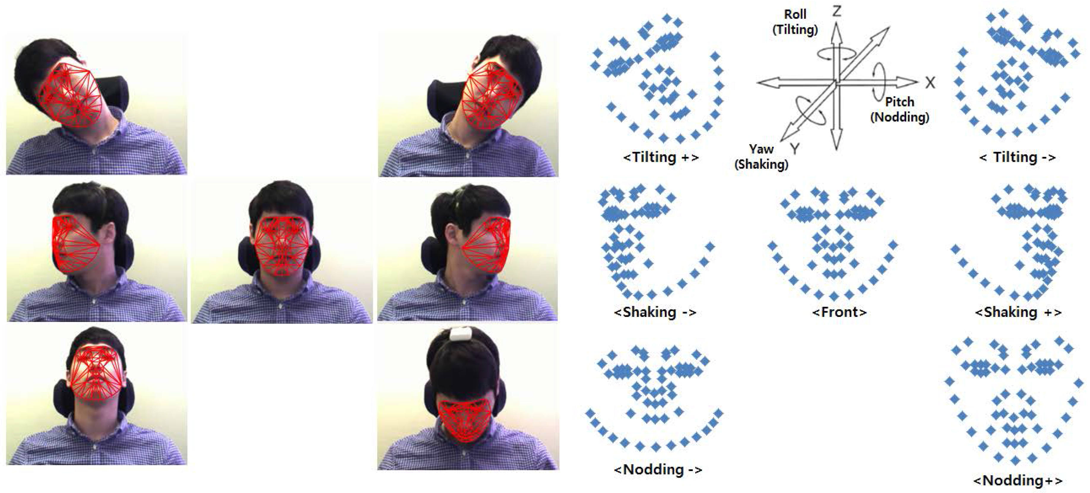
In this study, we have extended DB-ASM to include the extreme pose cases as illustrated in Figure 2, called it Pose Extended ASM (PE-ASM), where six extreme head poses are embedded into the basic model. On the right of the same figure, the center is the average shape model, and the other six shape models correspond to the extreme head pose cases, respectively. In other words, we have trained seven different DB-ASMs including the frontal face model. We have used the threshold values, as indicated in Table 1, in categorizing the head pose of the current face. In Section 3.1, it is shown that the POSIT algorithm is used in estimating the head pose of the given face. According to the estimated head pose value, the corresponding shape model is assigned among the seven head pose categories. Therefore, our face model is a head pose-specific model. Once the shape model is assigned, the face fitting starts with it and iterates until the error converges to a certain threshold.

3.3. Detection of Eye-Blink

It is known that when humans get drowsy, the blood is moving to the end of hands and feet, and the eyes are blinked more often because tear production in the lachrymal glands is reduced. In addition, the blood supply to the brain is also reduced. As a result of these, the person goes into a trance state as the brain activity is naturally reduced.
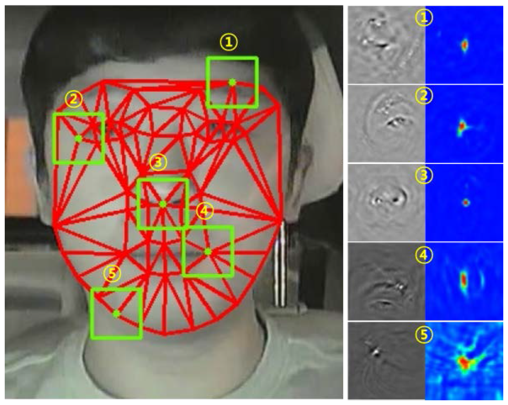
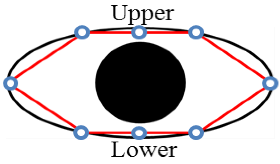
In the present study, eye-blink of the driver was counted based on the shape point around the eyes as shown in Figure 3. When the eye of a driver blinks, the upper and lower points naturally come closer to each other.
The number of blinks can be determined with the following equation. When d in Equation (11) is less than 80% to the maximum height of eyes, we consider it as a blink state. To make the ground truth of eye-blinking, three experts are employed: one for the judgment of blinking and two others for its verification.
d = ( U p p e r x L o w e r x ) 2 + ( U p p e r y L o w e r y ) 2

3.4. Hidden Markov Model for Drowsiness Detection

HMM can be classified into the following types upon the modeling of output probabilities: (1) HMM with discrete probabilities distribution predicts the observed output probabilities with the discrete characteristic of the state; (2) HMM with continuous probabilities distribution uses the probability density function allowing the use of a particular vector of error in the absence of a quantization process for a given output signal; and (3) HMM with semi-continuous distribution poses, combining the advantages of the two aforementioned models—the probability values in HMM with discrete probabilities and the probability density function in the HMM with the continuous probabilities distribution.
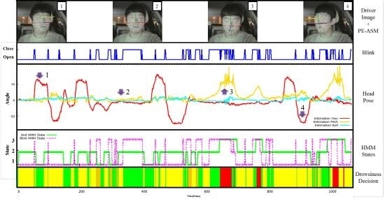
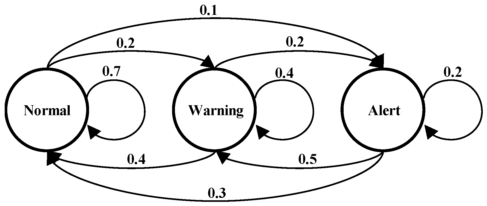
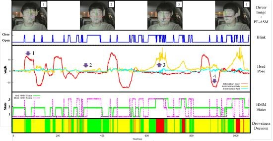
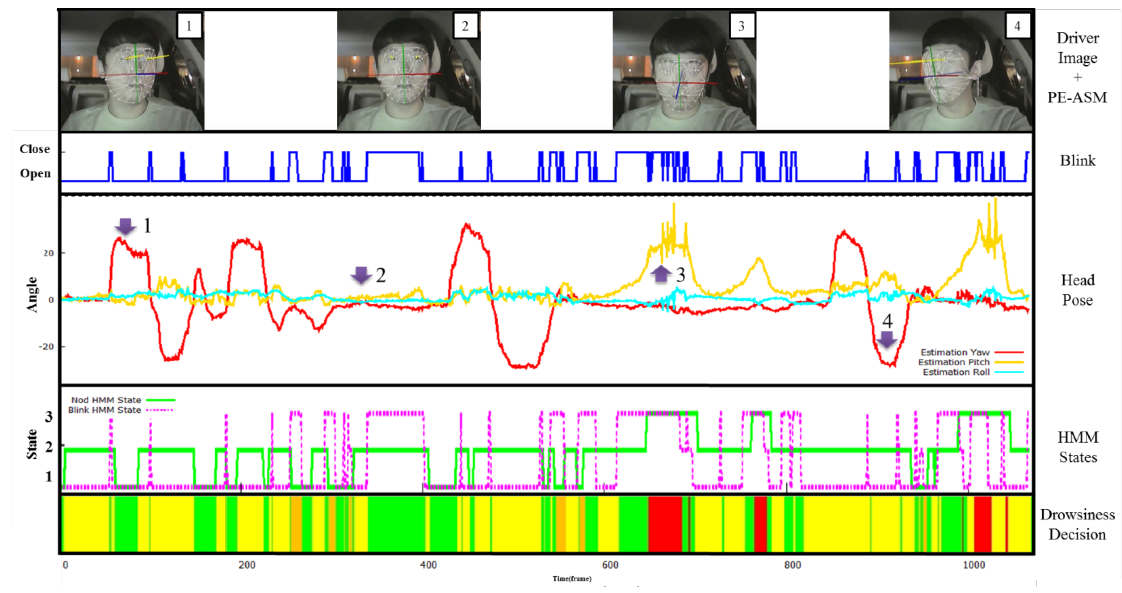
Figure 4 presents our HMM structure that consists of three different mental states of the driver. The head pose estimation and eye-blinking detection were used to create the HMM observation symbols and predict the probabilities of the parameter with the Baum-Welch algorithm, calculating the symbol state for each state. Here, it is considered that the transition probability and initial value of symbol probability at each state are equivalent when calculating the transition probability at each state. The predicted probability distribution, as well as the Viterbi algorithm, were used as a test sequence to obtain the sequence at the best state, selecting the best matching state.
For the present study, the GHMM (General Hidden Markov Model) public library, which is a standard HMM package, is used [
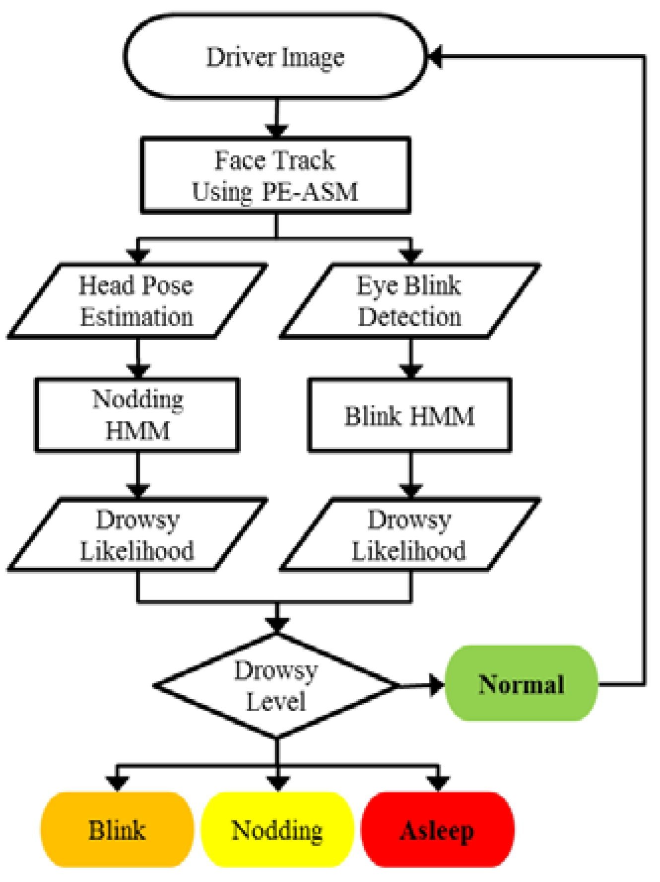
18]. The driver’s head position and eye-blinking output are used to predict the state most suitable to the driver’s state: one is an eye-blinking HMM and the other a nodding HMM, as shown in Figure 5. For training of the two HMMs, the videos are divided into many segments and each segment consists of 15 frames. The total is about 23,000 frames, and 70% of them are used for training and 30% of them for testing. The recognition rate during the training phase was 98% and during the testing phase was 92%. As training is carried out, the nodding and eye-blink states are enumerated to determine drowsy level of the given driver as shown in Figure 4. The mental state of the driver is categorized into: normal, warning, and alert. The state transition among the three states is determined by weights, as indicated in Figure 4.
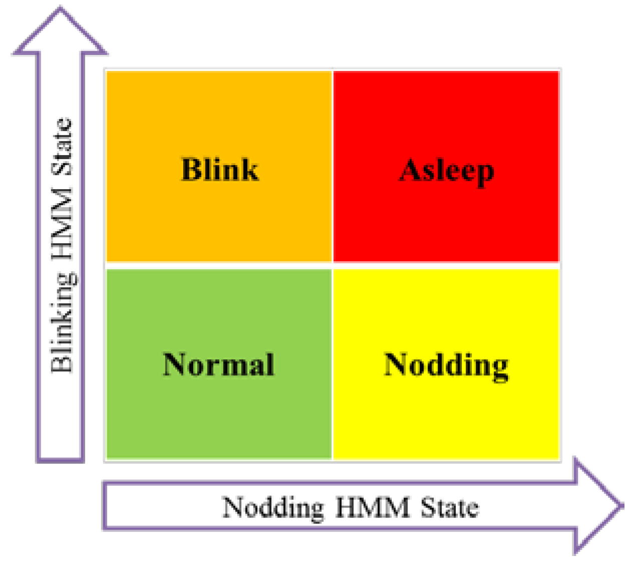
Figure 6 presents the criteria in determining the driver’s final mental state upon the variation of state. It is noticeable that when the eye-blinking and head nodding occur together, the system consider the driver’s state as asleep.

4. Experiments and Results

4.1. Comparision between AAM and DB-ASM

IMM Face DB was used to evaluate the performance of DB-ASM and AAM [19]. The Mean Absolute Error (MAE) and Root Mean Squared Error (RMSE) are used in measuring the fitting error. The former is defined in Equation (12). Here, n refers to the total frames and yi indicate the ground truth:
MAE =   1 n i = 1 n | f i y i | = 1 n i = 1 n | e i |
value for the pose, whereas fi refers to the estimated pose. The latter is defined as Equation (13).
RMSE ( s ) =   1 v i = 1 v ( s x i s g t x i ) 2 + ( s y i s g t y i ) 2
s g t = ground truth, s shape point.
Results indicate that DB-ASM outperforms AAM in terms of MAE as well as RMSE, as shown in Table 2, partly because DB-ASM is a recent face model. In any case, this is good news since we are going to adopt DB-ASM as our basic face model for the present study.
In addition, it is well known that DB-ASM is robust against partial occlusion cases. Our demonstration confirms that it is very reliable even against several occlusion cases, such as 20% and 40% occlusion, respectively, as illustrated in Figure 7. We have seen that the overall fitting is severely damaged when the same occlusions are applied to AAM.

4.2. Setup for Collecting Our Custom-Made Driving Database

Since our goal is to determine the driver's drowsiness using two drowsiness-related parameters, i.e., head nodding and eye-blink, we need a driving database that should be collected from a moving vehicle environment. However, it is not easy to collect such data simply because it could be very dangerous to manage sleepy drivers in the moving car. One possible solution is to let the subject drivers to simulate a drowsy driver in the vehicle according to the certain scenarios that may include a few drowsiness-related behaviors.
Two scenarios are prepared: the normal driving and the drowsy driving. For the former, the subject is supposed to look at the side and rear mirrors sporadically with a normal attentive forward viewing and, yet, to drive with natural blinking. For the latter, the subject blinks often, like a drowsy driver.
During the whole recording session, each subject wears a gyro sensor module mounted in a white box that is again attached to a black headband as shown to the left of Figure 8. The sensor is responsible to measure 3D head movement of the driver, and the collected data are sent on areal-time basis to the receiver, which connects to a notebook PC within the vehicle. This setup allows each subject to focus only on a given scenario, resulting in improved usability compared to the previous studies. We have collected two streams of video concurrently using two cameras: one for the color image and the other for black and white image. The former is used for the basis, whereas the latter works with an IR (infra-red) LED panel to dealing with the night driving. Each video was collected by synchronizing with the gyro-sensor. In building the DB, all videos are recorded with a 320 × 240 image size, 200 frames, and two different lighting conditions. On the right of Figure 8, the whole setup is installed in front of the driver in the vehicle. Figure 9 depicts four images taken during the database-building process. Table 3 shows the head pose ranges for pitch, roll, and yaw, respectively. Notice that the yaw angle is greater than other two head rotations because drivers mainly looking out the front window or at the two side mirrors while driving [20].
Our computing setup for analysis consists of i7 CPU with 4 GB main memory, and the software package includes visual studio 2010, OpenCV, and OpenMP. The face tracker based on the present DB-ASM runs at 16–20 frames/second, in the real-time basis.

4.3. Performance Comparision between PE-ASM and Other Face Models

The Boston University (BU) head pose DB [21] is the standard head pose dataset which provides ground truth of each subject’s head pose movements. It has been used in many previous studies in evaluating the head pose estimation task. However, the pose variation in the BU DB was not significant and, normally, it was less than 30°. Thus, it requires building a new database in which the range of head poses is large, as is often seen in the natural driving condition.
We have tested four face models such as AAM, ST-ASM, DB-ASM, and PE-ASM using the above two datasets. It is found that PE-ASM outperforms other three face models regarding the yaw fitting, which is the most important head pose component among three, for the BU DB case as shown in the top of Figure 10. Yet, performance between DB-ASM and PE-ASM for three components is not significant, which is in fact expected because the head pose ranges of BU DB are mostly less than 30°. The bottom panel of Figure 10 shows the result for our custom-made DB, where PE-ASM and DB-ASM outperform other two models in general. Notice that performance for the yaw is significantly improved with PE-ASM and DB-ASM. Overall performance of PE-ASM is better than that of DB-ASM, especially when the head pose is within the extreme head pose range.
Figure 11 illustrates the head pose estimations by AAM and PE-ASM, respectively. The top graphs (a,b) are obtained by applying two face models to BU DB, whereas the bottom ones (c,d) from our custom face DB. Given that the dotted lines in these graphs are the ground truth values, PE-ASM estimates the subject’s head pose reasonably well, whereas AAM cannot accommodate the extreme head cases. The blue arrows indicate when each subject made his head rotation. The top subject’s image came from BU DB, whereas the bottom one is from our custom-made face DB.

4.4. Inference of Drowsiness Using HMM

The result is illustrated in Figure 12 (and a video as a supplementary material), in which the top panel shows how PE-ASM runs, drawn as the warping grid on the driver’s face, and the head pose of the subject is indicated as yaw, pitch, and roll direction, respectively, calculated by POSIT algorithm. The second panel from the top shows the subject’s eye-blinking, and the third panel the moving head pose, as their graphs in time, respectively. Notice that when his head moves in the left or right direction, the yaw value increase as indicated in arrow (1) and (4) in the figure, whereas when he nods, the pitch value increases as indicated by the arrow (3). When he looks in the forward direction, three values approach zero as indicated by the arrow (2). The fourth panel shows the corresponding HMM states, i.e., eye-blinking and head nodding. The bottom panel depicts decision of drowsiness according to the HMM state transition diagram. Here the colors are coded as shown in Figure 6. Note that whenever the eye-blinking and the head nodding are overlapped, the red sign, i.e., asleep, is flashed.

5. Conclusions

The conventional driver drowsiness detection systems are vulnerable to extreme head rotation and occlusion. This study presents a new method to deal with such problems. First, it is shown that DB-ASM is more robust against occlusion than AAM; secondly, given that extreme head poses occur frequently during the natural driving condition in the car, PE-ASM is an extended version of DB-ASM by incorporating six extreme head pose cases into it. Evaluation result using BU face DB and our custom face DB suggests that it is particularly reliable against extreme head poses; thirdly, since our drowsiness detection system is based on the status of two facial features—head nodding and eye-blinking—it requires to make a judgment based on these information. HMMs are used in inferring whether the subject is drowsy or not in time sequence. It runs in the real-time basis on a PC. Our result suggests that it has a potential application in a commercial vehicle, in which the visual conditions are diverse and difficult to deal with.

Supplementary Materials

The following are available online at www.mdpi.com/2076-3417/6/5/137/s1, Video S1. This video demonstrates how both eye-bling and nodding of the driver are estimated and then Markov model makes inference according to their states in real-time.

Acknowledgments

This research was supported by Basic Science Research Program through the National Research Foundation of Korea (NRF) funded by the Ministry of Education, Science and Technology (NRF-2013R1A1A2006969) and by the MSIP (Ministry of Science, ICT and Future Planning), Korea, under the Global IT Talent support program (IITP-2015-R0134-15-1032) supervised by the IITP (Institute for Information and Communication Technology Promotion).

Author Contributions

In-Ho Choi and Yong-Guk Kim conceived and designed the experiments; In-Ho Choi and Chan-Hee Jeong collected the driving database; Yong-Guk Kim wrote the paper.

Conflicts of Interest

The authors declare no conflict of interest.

References

  1. U.S. Department of Transportation. Intelligent Vehicle Initiative 2002 Annual Report; Washington, Wa, USA, 2002.
  2. Dong, Y.; Hu, Z.; Uchimura, K.; Murayama, N. Driver inattention monitoring system for intelligent vehicles: A review. In IEEE Transactions on Intelligent Transportation Systems; IEEE: New York, NY, USA, 2011; Volume 12, pp. 596–614. [Google Scholar]
  3. Cootes, T.F.; Taylor, C.J. Combining point distribution models with shape models based on finite element analysis. Image Vis. Comput. 1995, 13, 403–409. [Google Scholar] [CrossRef]
  4. Cootes, T.F.; Taylor, C.J. Statistical Models of Appearance for Computer Vision. 2004. [Google Scholar]
  5. Cootes, T.F.; Edwards, G.J.; Taylor, C.J. Active appearance models. In IEEE Transactions on Pattern Analysis and Machine Intelligence; IEEE: New York, NY, USA, 2001; Volume 6, pp. 681–685. [Google Scholar]
  6. Matthews, I.; Baker, S. Active appearance models revisited. Int. J. Comput. Vis. 2004, 60, 135–164. [Google Scholar] [CrossRef]
  7. Cho, K.S.; Choi, I.H.; Kim, Y.G. Robust facial expression recognition using a smartphone working against illumination variation. Appl. Math. Inf. Sci. 2012, 6, 403S–408S. [Google Scholar]
  8. Cristinacce, D.; Cootes, T. Feature Detection and Tracking with Constrained Local Models. BMVC 2006, 2. [Google Scholar] [CrossRef]
  9. Martins, P.; Caseiro, R.; Henriques, J.F.; Batista, J. Discriminative Bayesian active shape models. In Computer Vision–ECCV 2012; Springer: Berlin, Germany; Heidelberg, Germany, 2012; pp. 57–70. [Google Scholar]
  10. Martins, P.; Henriques, J.F.; Caseiro, R.; Batista, J. Bayesian Constrained Local Models Revisited. In IEEE Transactions on Pattern Analysis and Machine Intelligence; IEEE: New York, NY, USA, 2016; Volume 38. [Google Scholar]
  11. Dementhon, D.F.; Davis, L.S. Model-based object pose in 25 lines of code. Int. J. Comput. Vis. 1995, 15, 123–141. [Google Scholar] [CrossRef]
  12. Ji, Q.; Yang, X. Real-time eye, gaze, and face pose tracking for monitoring driver vigilance. Real Time Imaging 2002, 8, 357–377. [Google Scholar] [CrossRef]
  13. Mbouna, R.; Kong, K.; Chun, M. Visual analysis of eye state and head pose for driver alertness monitoring. In IEEE Transactions on Intelligent Transfortational Systems; IEEE: New York, NY, USA, 2013; Volume 14. [Google Scholar]
  14. Rabiner, L. A tutorial on hidden Markov models and selected applications in speech recognition. In Proceedings of the IEEE; IEEE: New York, NY, USA, 1989; Volume 77, pp. 257–286. [Google Scholar]
  15. Barci, A.M.; Ansari, R.; Khokhar, A.; Cetin, E. Eye tracking using Markov models. In Proceedings of the 17th International Conference on ICPR 2004 Pattern Recognition, New York, NY, USA, 23–26 August 2004; IEEE: New York, NY, USA, 2004; Volume 3. [Google Scholar]
  16. Sathyanarayana, A.; Boyraz, P.; Hansen, J. Driver behavior analysis and route recognition by Hidden Markov Models. In Proceedings of the IEEE International Conference on Vehicular Electronics and Safety, Columbus, OH, USA, 22–24 September 2008.
  17. Bolme, D.S.; Beveridge, J.R.; Draper, B.A.; Lui, Y.M. Visual object tracking using adaptive correlation filters. In Proceedings of the 2010 IEEE Conference on Computer Vision and Pattern Recognition (CVPR), San Francisco, CA, USA, 13–18 June 2010; pp. 2544–2550.
  18. General Hidden Markov Model library (GHMM). Available online: http://ghmm.org/ (accessed on 9 August 2013).
  19. Nordstrøm, M.M.; Larsen, M.; Sierakowski, J.; Stegmann, M.B. The IMM Face Database-an Annotated Dataset of 240 Face Images; Technical University of Denmark: Copenhagen, Denmark, 2004. [Google Scholar]
  20. Kim, C.; Kim, D.K.; Kho, S.Y.; Kang, S.; Chung, K. Dynamically Determining the Toll Plaza Capacity by Monitoring Approaching Traffic Conditions in Real-Time. Appl. Sci. 2016, 6, 87. [Google Scholar] [CrossRef]
  21. La Cascia, M.; Isidoro, J.; Sclaroff, S. Head tracking via robust registration in texture map images. In Proceedings of the IEEE Computer Society Conference on Computer Vision and Pattern Recognition, Santa Barbara, CA, USA, 23–25 June 1998; pp. 508–514.
Figure 1. Appearance of MOSSE (Minimum Output Sum of Squared Error)filter and response map on a PDM (Point Distribution Model)shape: the PDM shape on a given face having 56 landmarks (left); the MOSSE filters at five sampled locations (middle); and their corresponding response maps (right).
Applsci 06 00137 g001
Figure 2. Pose Extended Active Shape Model (PE-ASM) is applied to the six extreme pose cases (Left) and their corresponding shape models are drawn (Right). Here, the ‘Front’ case covers the head rotation range from −30° to +30° in three different axis, and the other six cases cover the extreme head rotation occasions as given in Table 1.
Applsci 06 00137 g002
Figure 3. The geometric model for the eye.
Applsci 06 00137 g003
Figure 4. Markov model state transition diagram in which there are three possible states, and state transition occurs according to the transition weights, as indicated.
Applsci 06 00137 g004
Figure 5. System Flow Chart.
Applsci 06 00137 g005
Figure 6. The criteria for determining driver’s state upon changes in nodding and blinking HMM (Hidden Markov Model)states.
Applsci 06 00137 g006
Figure 7. Robust fitting of DB-ASM against several occlusion cases.
Applsci 06 00137 g007
Figure 8. A wireless gyro-sensor module mounted in a white box and its receiver (left), and cameras and other setup installed in the vehicle (right).
Applsci 06 00137 g008
Figure 9. Images for four subjects taken from our custom-made driving face database. The driver often nods without looking at the side and rear mirrors. In our custom-made DB, subjects are asked to move their head to the extreme head poses while driving naturally. The yaw, pitch, and roll of the extreme poses are greater than 30° for four subjects and the image size is 640 × 480 with 500 frames length for each case.
Applsci 06 00137 g009
Figure 10. Performance comparison between four face models using BU DB (Boston University database) (top) and our custom-made database (bottom). Three different head rotations are indicated with blue, red, and green, respectively.
Applsci 06 00137 g010
Figure 11. Illustration of head pose estimation with AAM and PE-ASM using BU DB (a,b) and our custom DB (c,d), respectively. GT indicates the ground truth. The blue arrow indicates the time when each subject made his head rotation. Note that PE-ASM follows ground truth better than AAM, although it has some noise.
Applsci 06 00137 g011
Figure 12. Detection of driver’s drowsiness using PE-ASM (Pose Extended – Active Shape Model) and HMM: PE-ASM is applied to the images of a driver (top panel), eye-blinking (2nd panel), head pose (3rd panel), HMM states (4th panel) and the decision of driver’s drowsiness (bottom panel). Note that whenever blinking and nodding HMM states are overlapped, the system detects drowsiness of the driver, indicated as red rectangles, as shown in the bottom panel.
Applsci 06 00137 g012
Table 1. Categorization of head pose ranges of our dataset into 6 extremes cases.
Yaw−−54~−15+15~75Yaw+
Pitch−−30~−15+15~39Pitch+
Roll−−46~−15+15~52Roll+
Table 2. Comparison of fitting performance between AAM (Active Appearance Model)and DB-ASM (Discriminative Bayesian-Active Shape Model).
Face ModelMAERMSE
DB-ASM8.4228811.08351
AAM11.5148213.04523
Table 3. Head pose ranges of four subjects in our custom-made face database.
ValuePitchRollYaw
Min−30.9305−46.0244−54.5366
Max39.436052.227575.1661

