Dynamics of a Stochastic Intraguild Predation Model

Abstract

Intraguild predation (IGP) is a widespread ecological phenomenon which occurs when one predator species attacks another predator species with which it competes for a shared prey species. The objective of this paper is to study the dynamical properties of a stochastic intraguild predation model. We analyze stochastic persistence and extinction of the stochastic IGP model containing five cases and establish the sufficient criteria for global asymptotic stability of the positive solutions. This study shows that it is possible for the coexistence of three species under the influence of environmental noise, and that the noise may have a positive effect for IGP species. A stationary distribution of the stochastic IGP model is established and it has the ergodic property, suggesting that the time average of population size with the development of time is equal to the stationary distribution in space. Finally, we show that our results may be extended to two well-known biological systems: food chains and exploitative competition.

1. Introduction

Interactions among species can structure biological communities by affecting the identity, number and abundance of species present. Intraguild predation (IGP) has been playing an important role in structuring ecological communities, strongly influencing the structure and function of food webs. IGP describes an interaction in which one predator species consumes another predator species with whom it also competes for shared prey [1,2]. This suggests that IGP combines two important structuring forces in ecological communities: competition and predation. Accordingly, IGP is not only a taxonomically widespread interaction within communities which can occur at different trophic levels, but also a central force to forecast the stability of food webs and the maintenance of biodiversity.

The simplest form of IGP is depicted by a simple food web model in which IGP can occur: a top predator (IG predator P), an intermediate consumer (IG prey N), and a shared prey (R). The development of IGP model can be traced back to Holt and Polis [1] who initially introduce a three species model with the Lotka–Volterra type to study the species coexistence of IGP and point out that it is very difficult to achieve a stable three-species steady state. After that, there are some articles to consider an IGP model with different structures and forms, such as, IGP model with the Lotka–Volterra type [3,4,5], the IGP model with special forms of the functional and numerical responses [6,7,8], the IGP model with prey switching or adaptive prey behavior [9,10], and the IGP model with generalist predator or time delay [11,12,13].

The effect of the random variation of environment is an integral part of any realistic ecosystem. Stochastic models may be more important in characterizing population dynamics in contrast to the deterministic models. In essence, random factors can lead to complete extinction of populations even if the population size is relatively large. Previous studies have explored the dynamic properties for stochastic single species models [14,15,16], stochastic predator–prey models [17,18,19,20,21,22,23], stochastic competitive models [24,25,26,27], stochastic mutualism model [28,29,30,31]. Specially, Liu and Wang [32] investigated a two-prey one-predator model with random perturbations. However, there are few studies to investigate dynamics of a stochastic IGP model.

Motivated by the existing nice studies and the above considerations, we consider a following IGP model with the Lotka–Volterra type

$$\begin{array}{cc}\hfill \frac{dR\left(t\right)}{dt}& =R\left(t\right)(r-a_{rr}R\left(t\right)-a_{rn}N\left(t\right)-a_{rp}P\left(t\right)),\hfill \\ \hfill \frac{dN\left(t\right)}{dt}& =N\left(t\right)(-d_n+e_{rn}{a}_{rn}R\left(t\right)-a_{nn}N\left(t\right)-a_{np}P\left(t\right)),\hfill \\ \hfill \frac{dP\left(t\right)}{dt}& =P\left(t\right)(-d_p+e_{rp}{a}_{rp}R\left(t\right)+e_{np}{a}_{np}N\left(t\right)-a_{pp}P\left(t\right)),\hfill \end{array}$$

(1)

where $R\left(t\right),N\left(t\right)$ and $P\left(t\right)$ are the densities of the shared prey, IG prey and IG predator, respectively; r is the per capita growth rate of the shared prey and $d_i(i=n,p)$ is the death rate of species i; $a_{ii}(i=r,n,p)$ is the intraspecific competition rate of species i; $a_{rp}$ and $a_{np}$ are the predation rates of IG predator to the shared prey and IG prey; $a_{rn}$ is the predation rate of IG prey to the shared prey; $e_{ij}(i=r,n,j=n,p)$ is the conversion rates of resource consumption into reproduction for IG prey and IG predator. Here, $a_{rn},a_{rp},a_{np}$ is nonnegative constants and the remaining parameters are all positive constants. In view of the fact that the per capita growth rate and the death rate exhibit random fluctuation to a greater or lesser extent (see [33]), we assume that the environmental fluctuation mainly affects the parameters r, $d_n$ and $d_p$ and model these fluctuations by means of independent Gaussian white noises. Let ${(B_r\left(t\right),B_n\left(t\right),B_p\left(t\right))}^T$ be a three-dimensional Brownian motion defined on a complete probability space $(\Omega ,\mathcal{F},\mathcal{P})$ and

$$r\to r+{\alpha }_r{\dot{B}}_r\left(t\right),d_n\to d_n-{\alpha }_n{\dot{B}}_n\left(t\right),d_p\to d_p-{\alpha }_p{\dot{B}}_p\left(t\right),$$

(2)

where ${\alpha }_r^2,{\alpha }_n^2,{\alpha }_p^2$ are the intensity of the white noise. Thus we consider the Itô’s stochastic IGP model as follows:

$$\begin{array}{cc}\hfill dR\left(t\right)& =R\left(t\right)(r-a_{rr}R\left(t\right)-a_{rn}N\left(t\right)-a_{rp}P\left(t\right))dt+{\alpha }_{r}R\left(t\right)d{B}_r\left(t\right),\hfill \\ \hfill dN\left(t\right)& =N\left(t\right)(-d_n+e_{rn}{a}_{rn}R\left(t\right)-a_{nn}N\left(t\right)-a_{np}P\left(t\right))dt+{\alpha }_{n}N\left(t\right)d{B}_n\left(t\right),\hfill \\ \hfill dP\left(t\right)& =P\left(t\right)(-d_p+e_{rp}{a}_{rp}R\left(t\right)+e_{np}{a}_{np}N\left(t\right)-a_{pp}P\left(t\right))dt+{\alpha }_{p}P\left(t\right)d{B}_p\left(t\right).\hfill \end{array}$$

(3)

The main aim of this paper is to study the dynamics of the model (3). Theoretical studies have suggested that it is very difficult to a achieve stable three-species steady state for the deterministic IGP model. Hence, the first interesting topic of the present paper is whether we can establish a criterion for three- species coexistence under the influence of environmental noise and give the sufficient conditions for global asymptotic stability of the positive solution of model (3). Another important and interesting problem is whether there is a stationary distribution of the stochastic IGP model (3) and if it has the ergodic property.

The rest of the paper is organized as follows. In the next section, we do some necessary preparations including some notations and several important lemmas. In Section 3, we explore stochastic persistence and the extinction of model (3) for five different cases and compare them with the corresponding results of the deterministic model (1).

Then, we establish global asymptotic stability of the positive solution of the model (3). In Section 4, we prove that there is a stationary distribution of model (3), and it has the ergodic property by using the theory of Has’minskii [34]. In the final section, according to the conclusions of previous sections, we first study dynamic properties of two well-known biological systems under random perturbations: food chains and exploitative competition. We state biological implications of our mathematical findings and present some figures to illustrate or complement our mathematical findings.

2. Preliminaries

In this section, we first introduce several important lemmas.

Lemma 1 

(see [32]). Let $z\in C(\Omega \times [0,+\infty ),{\mathbb{R}}_{+})$, ${\displaystyle {\left[z\right]}^{*}=\underset{t\to +\infty }{lim\; sup}\frac{1}{t}{\int }_0^{t}z\left(s\right)ds}$ and ${\displaystyle {\left[z\right]}_{*}=\underset{t\to +\infty }{lim\; inf}\frac{1}{t}{\int }_0^{t}z\left(s\right)ds}$.

(i)

If there exist two positive constants T and ${\lambda }_0$ such that

$$lnz\left(t\right)\le \lambda t-{\lambda }_0{\int }_0^{t}z\left(s\right)ds+\sum _{i=1}^n{\sigma }_i{B}_i\left(t\right)$$

(4)

for all $t\ge T,$ where $B_i\left(t\right)$, $1\le i\le n$, are independent standard Brownian motions and ${\sigma }_i$, $1\le i\le n$, are constants, then ${\displaystyle {\left[z\right]}^{*}\le \lambda /{\lambda }_{0}a.s.}$ if $\lambda \ge 0$ or $\underset{t\to +\infty }{lim}z\left(t\right)=0a.s.$ if $\lambda <0.$

(ii)

If there exist three positive constants T, λ, and ${\lambda }_0$ such that

$$lnz\left(t\right)\ge \lambda t-{\lambda }_0{\int }_0^{t}z\left(s\right)ds+\sum _{i=1}^n{\sigma }_i{B}_i\left(t\right)$$

(5)

for all $t\ge T,$ where $B_i\left(t\right)$, $1\le i\le n$, are independent standard Browniam motions and ${\sigma }_i$, $1\le i\le n$, are constants, then ${\left[z\right]}_{*}\ge {\lambda }_{0}a.s.$

Similar to Theorem 2.1, Lemma 3.1 and Lemma 3.4 in [25], we have the following lemma:

Lemma 2. 

For any given initial value ${(R\left(0\right),N\left(0\right),P\left(0\right))}^T\in {\mathbb{R}}_{+}^3$ and any $p>0$, model (3) has a unique solution ${(R\left(t\right),N\left(t\right),P\left(t\right))}^T$ on $t\ge 0$ which will remain in ${\mathbb{R}}_{+}^3$ with probability 1 and there is a constant $K=K\left(p\right)$ such that

$$\underset{t\to +\infty }{lim\; sup}E\left(R{\left(t\right)}^p\right)\le K,\underset{t\to +\infty }{lim\; sup}E\left(N{\left(t\right)}^p\right)\le K,\underset{t\to +\infty }{lim\; sup}E\left(P{\left(t\right)}^p\right)\le K.$$

(6)

Moreover, the solution ${(R\left(t\right),N\left(t\right),P\left(t\right))}^T$ of (3) has the properties that

$$\underset{t\to +\infty }{lim\; sup}\frac{lnR\left(t\right)}{lnt}\le 1a.s.,\underset{t\to +\infty }{lim\; sup}\frac{lnN\left(t\right)}{lnt}\le 1a.s.,\underset{t\to +\infty }{lim\; sup}\frac{lnP\left(t\right)}{lnt}\le 1a.s.$$

(7)

In order to obtain the conditions of global asymptotic stability of solutions for the stochastic model (3), we need the following two lemmas.

Lemma 3 

(see [35]). If there exist positive constants ${\omega }_1,{\omega }_2$ and κ such that an n-dimensional stochastic process $Y\left(t\right)$, $t\ge 0$ satisfies

$${E|Y\left(t\right)-Y\left(s\right)|}^{{\omega }_1}\le \kappa {|t-s|}^{1+{\omega }_2}$$

(8)

for $0\le t,s<+\infty$, then there exists a continuous modification $\overline{Y}\left(t\right)$ of $Y\left(t\right)$ such that for every $\omega \in (0,{\omega }_1/{\omega }_2)$ there is a positive random variable $h\left(\omega \right)$ such that

$$P\left\{{\displaystyle \underset{\genfrac{}{}{0pt}{}{0<|t-s|<h\left(\omega \right)}{0\le t,s<+\infty }}{sup}\frac{|\overline{Y}(t,\omega )-Y(s,\omega )|}{{|t-s|}^{\omega }}\le \frac{2}{1-2^{-\omega }}}\right\}=1,$$

(9)

which implies that almost every sample path of $\overline{Y}\left(t\right)$ is locally but uniformly Hölder continuous with exponent ω.

Lemma 4 

(see [36]). If g is a non-negative function defined on $[0,+\infty )$ such that g is integrable and is uniformly continuous, then $\underset{t\to +\infty }{lim}g\left(t\right)=0.$

To establish the existence of a stationary distribution of model (3) in Section 4, we introduce the theory of Has’minskii [34] and let $Y\left(t\right)$ be a homogeneous Markov process in $E^l$ ($E^l$ is an l-dimensional Euclidean space) described by the stochastic equation

$$dY\left(t\right)=b\left(Y\right)dt+\sum _{m=1}^k{g}_m\left(Y\right)d{B}_m\left(t\right).$$

(10)

Let the diffusion matrix be $\Lambda \left(x\right)=\left(a_{ij}\left(x\right)\right)$, $a_{ij}\left(x\right)={\sum }_{m=1}^k{g}_m^i\left(x\right)g_m^j\left(x\right)$.

Assumption 5. 

There is a bounded domain $U\subset E^l$ with regular boundary Γ such that

(H${}_1$)

In the domain U and some neighborhood thereof, the smallest eigenvalue of the diffusion matrix $\Lambda \left(x\right)$ is bounded away from zero;

(H${}_2$)

If $x\in E^l\backslash U$, the mean time τ at which a path issuing from x reaches the set U is finite, and ${sup}_{x\in K}{E}_x\tau <+\infty$ for every compact subset $K\subset E^l$.

It is worth noting that we can use the following two stronger conditions to verify (H${}_1$) and (H${}_2$) in Assumption 5:

(K${}_1$)

To obtain (H${}_1$), we only need to show that T is uniformly elliptical in U, where $Tu=b\left(x\right)u_x+tr(\Lambda \left(x\right)u_{xx})/2$, that is, there exists a $c>0$ such that ${\sum }_{i,j=1}^k{a}_{ij}\left(x\right){\xi }_i{\xi }_j\ge c{\left|\xi \right|}^2$, $x\in U$, $\xi \in R^l$ (see [37,38]);

(K${}_2$)

To obtain (H${}_2$), we only need to prove that there exist a neighborhood U and a nonnegative $C^2$-function $V\left(x\right)$ such that for any $x\in E^l\backslash U$, $LV\left(x\right)<0$ (see [39]).

Lemma 6 

([34]). If Assumption 5 holds, then the Markov process $Y\left(t\right)$ has a stationary distribution $\mu (·)$. Moreover, if $f(·)$ is a function integrable with respect to the measure μ, then

$${\displaystyle P\left\{\underset{t\to +\infty }{lim}\frac{1}{t}{\int }_0^{t}f\left(Y\left(s\right)\right)ds={\int }_{E^l}f\left(x\right)\mu \left(dx\right)\right\}=1.}$$

(11)

In order to study dynamic properties of model (3), we do the following notations:

$$\left[g\left(t\right)\right]=\frac{1}{t}{\int }_0^{t}g\left(s\right)ds,{\left[g\right]}^{*}=\underset{t\to +\infty }{lim\; sup}\frac{1}{t}{\int }_0^{t}g\left(s\right)ds,{\left[g\right]}_{*}=\underset{t\to +\infty }{lim\; inf}\frac{1}{t}{\int }_0^{t}g\left(s\right)ds;$$

(12)

$$\begin{array}{cc}\hfill L& =\left|\begin{array}{ccc}{a}_{rr}& a_{rn}& a_{rp}\\ -e_{rn}{a}_{rn}& a_{nn}& a_{np}\\ -e_{rp}{a}_{rp}& -e_{np}{a}_{np}& a_{pp}\end{array}\right|,M=\left|\begin{array}{ccc}{a}_{rr}& r& {\alpha }_r^2/2\\ -e_{rn}{a}_{rn}& -d_n& {\alpha }_n^2/2\\ -e_{rp}{a}_{rp}& -d_p& {\alpha }_p^2/2\end{array}\right|;\hfill \\ \hfill L_1& =\left|\begin{array}{ccc}r& a_{rn}& a_{rp}\\ -d_n& a_{nn}& a_{np}\\ -d_p& -e_{np}{a}_{np}& a_{pp}\end{array}\right|,M_1=\left|\begin{array}{ccc}{\alpha }_r^2/2& a_{rn}& a_{rp}\\ {\alpha }_n^2/2& a_{nn}& a_{np}\\ {\alpha }_p^2/2& -e_{np}{a}_{np}& a_{pp}\end{array}\right|;\hfill \\ \hfill L_2& =\left|\begin{array}{ccc}{a}_{rr}& r& a_{rp}\\ -e_{rn}{a}_{rn}& -d_n& a_{np}\\ -e_{rp}{a}_{rp}& -d_p& a_{pp}\end{array}\right|,M_2=\left|\begin{array}{ccc}{a}_{rr}& {\alpha }_r^2/2& a_{rp}\\ -e_{rn}{a}_{rn}& {\alpha }_n^2/2& a_{np}\\ -e_{rp}{a}_{rp}& {\alpha }_p^2/2& a_{pp}\end{array}\right|;\hfill \\ \hfill L_3& =\left|\begin{array}{ccc}{a}_{rr}& a_{rn}& r\\ -e_{rn}{a}_{rn}& a_{nn}& -d_n\\ -e_{rp}{a}_{rp}& -e_{np}{a}_{np}& -d_p\end{array}\right|,M_3=\left|\begin{array}{ccc}{a}_{rr}& a_{rn}& {\alpha }_r^2/2\\ -e_{rn}{a}_{rn}& a_{nn}& {\alpha }_n^2/2\\ -e_{rp}{a}_{rp}& -e_{np}{a}_{np}& {\alpha }_p^2/2\end{array}\right|.\hfill \end{array}$$

(13)

3. Stochastic Persistence and Stochastic Extinction

To illuminate the effect of the stochastic perturbations for population and compare the stochastic IGP model (3) with the deterministic IGP model (1), we first explore the existence and local stability of boundary and positive equilibria for model (1). The summary of conditions for the existence and local stability of equilibria are listed in Table 1.

Table 1. Existence and local stability of equilibria for model (1).

Equilibria	Existence	Local Stability
$E_0(0,0,0)$	Always	Never
$E_r(r/a_{rr},0,0)$	Always	${\delta }_5<0,{\delta }_6<0$
$E_{rn}({\delta }_4/{\delta }_1,{\delta }_5/{\delta }_1,0)$	${\delta }_5>0$	$L_3<0$
$E_{rp}({\delta }_3/{\delta }_2,0,{\delta }_6/{\delta }_2)$	${\delta }_6>0$	$L_2<0$
$E_{rnp}(L_1/L,L_2/L,L_3/L)$	$L>0,L_i>0,i=1,2,3$	${\delta }_1{\delta }_2+{\delta }_7{\delta }_8>0$

$Here,{\delta }_1=a_{rr}{a}_{nn}+e_{rn}{a}_{rn}^2;{\delta }_2=a_{rr}{a}_{pp}+e_{rp}{a}_{rp}^2;{\delta }_3=r{a}_{pp}+a_{rp}{d}_p;{\delta }_4=r{a}_{nn}+a_{rn}{d}_n;{\delta }_5=-a_{rr}{d}_n+r{e}_{rn}{a}_{rn};{\delta }_6=-a_{rr}{d}_p+r{e}_{rp}{a}_{rp};{\delta }_7=-a_{rr}{e}_{np}{a}_{np}+a_{rn}{e}_{rp}{a}_{rp};{\delta }_8=a_{rr}{a}_{np}+a_{rp}{e}_{rn}{a}_{rn}.$

Now, we analyze stochastic persistence and stochastic extinction of model (3).

Definition 7 

(see [32]). Species $x\left(t\right)$ is said to be persistent in the mean if ${\left[x\right]}_{*}>0$.

Let

$$\begin{array}{cc}\hfill {\overline{\delta }}_1& ={\alpha }_r^2{a}_{nn}/2-{\alpha }_n^2{a}_{rn}/2,{\overline{\delta }}_2={\alpha }_r^2{a}_{pp}/2-{\alpha }_p^2{a}_{rp}/2,\hfill \\ \hfill {\overline{\delta }}_3& ={\alpha }_n^2{a}_{rr}/2+{\alpha }_r^2{e}_{rn}{a}_{rn}/2,{\overline{\delta }}_4={\alpha }_p^2{a}_{rr}/2+{\alpha }_r^2{e}_{rp}{a}_{rp}/2.\hfill \end{array}$$

(14)

A direct calculation gives

$$\begin{array}{cc}\hfill 2r/{\alpha }_r^2-{\delta }_5/{\overline{\delta }}_3& =a_{rr}(r{\alpha }_n^2+d_n{\alpha }_r^2)/\left({\alpha }_r^2{\overline{\delta }}_3\right)>0,\hfill \\ \hfill 2r/{\alpha }_r^2-{\delta }_6/{\overline{\delta }}_4& =a_{rr}(r{\alpha }_p^2+d_p{\alpha }_r^2)/\left({\alpha }_r^2{\overline{\delta }}_4\right)>0,\hfill \\ \hfill {\delta }_4/{\overline{\delta }}_1-2r/{\alpha }_r^2& =a_{rn}(r{\alpha }_n^2+d_n{\alpha }_r^2)/\left({\overline{\delta }}_1{\alpha }_r^2\right)>0,\hfill \\ \hfill {\delta }_3/{\overline{\delta }}_2-2r/{\alpha }_r^2& =a_{rp}(r{\alpha }_p^2+d_p{\alpha }_p^2)/\left({\overline{\delta }}_2{\alpha }_r^2\right)>0.\hfill \end{array}$$

(15)

Theorem 8. 

The following five cases hold:

(i)

If $2r<{\alpha }_r^2$, then all the populations are extinction a.s.

(ii)

If $2r/{\alpha }_r^2>1>max\{{\delta }_5/{\overline{\delta }}_3,{\delta }_6/{\overline{\delta }}_4\}$, then $N\left(t\right)$ and $P\left(t\right)$ are extinction a.s. and

$${\displaystyle \underset{t\to +\infty }{lim}\frac{1}{t}{\int }_0^{t}R\left(s\right)ds=\frac{r-{\alpha }_r^2/2}{a_{rr}}a.s.}$$

(16)

(iii)

If $L>0$, ${\delta }_5/{\overline{\delta }}_3>1$ and $L_3<M_3$, then $P\left(t\right)$ is extinction a.s. and

$$\begin{array}{cc}\hfill {\displaystyle \underset{t\to +\infty }{lim}\frac{1}{t}{\int }_0^{t}R\left(s\right)ds}& =\frac{{\delta }_4-{\overline{\delta }}_1}{{\delta }_1}a.s.,\hfill \\ \hfill {\displaystyle \underset{t\to +\infty }{lim}\frac{1}{t}{\int }_0^{t}N\left(s\right)ds}& =\frac{{\delta }_5-{\overline{\delta }}_3}{{\delta }_1}a.s.\hfill \end{array}$$

(17)

(iv)

If $L>0$, ${\delta }_6/{\overline{\delta }}_4>1$ and $L_2<M_2$, then $N\left(t\right)$ is extinction a.s. and

$$\begin{array}{cc}\hfill {\displaystyle \underset{t\to +\infty }{lim}\frac{1}{t}{\int }_0^{t}R\left(s\right)ds}& =\frac{{\delta }_3-{\overline{\delta }}_2}{{\delta }_2}a.s.,\hfill \\ \hfill {\displaystyle \underset{t\to +\infty }{lim}\frac{1}{t}{\int }_0^{t}P\left(s\right)ds}& =\frac{{\delta }_6-{\overline{\delta }}_4}{{\delta }_2}a.s.\hfill \end{array}$$

(18)

(v)

If $L>0$, $L_i>M_i$, $i=1,2,3$, then

$$\begin{array}{cc}\hfill {\displaystyle \underset{t\to +\infty }{lim}\frac{1}{t}{\int }_0^{t}R\left(s\right)ds}& =\frac{L_1-M_1}{L}a.s.,\hfill \\ \hfill {\displaystyle \underset{t\to +\infty }{lim}\frac{1}{t}{\int }_0^{t}N\left(s\right)ds}& =\frac{L_2-M_2}{L}a.s.,\hfill \\ \hfill {\displaystyle \underset{t\to +\infty }{lim}\frac{1}{t}{\int }_0^{t}P\left(s\right)ds}& =\frac{L_3-M_3}{L}a.s.\hfill \end{array}$$

(19)

Proof. 

It follows from Itô’s formula that

$$\begin{array}{cc}\hfill dlnR& =(r-{\alpha }_r^2/2-a_{rr}R\left(t\right)-a_{rn}N\left(t\right)-a_{rp}P\left(t\right))dt+{\alpha }_{r}d{B}_r\left(t\right),\hfill \\ \hfill dlnN& =(-d_n-{\alpha }_n^2/2+e_{rn}{a}_{rn}R\left(t\right)-a_{nn}N\left(t\right)-a_{np}P\left(t\right))dt+{\alpha }_{n}d{B}_n\left(t\right),\hfill \\ \hfill dlnP& =(-d_p-{\alpha }_p^2/2+e_{rp}{a}_{rp}R\left(t\right)+e_{np}{a}_{np}N\left(t\right)-a_{pp}P\left(t\right))dt+{\alpha }_{p}d{B}_p\left(t\right).\hfill \end{array}$$

(20)

By integrating from 0 to t on both sides of the above equation and dividing by t, we have

$$\begin{array}{cc}\hfill {\displaystyle \frac{1}{t}ln\frac{R\left(t\right)}{R\left(0\right)}}& {\displaystyle =r-\frac{{\alpha }_r^2}{2}-a_{rr}\left[R\left(t\right)\right]-a_{rn}\left[N\left(t\right)\right]-a_{rp}\left[P\left(t\right)\right]+\frac{{\alpha }_r{B}_r\left(t\right)}{t},}\hfill \\ \hfill {\displaystyle \frac{1}{t}ln\frac{N\left(t\right)}{N\left(0\right)}}& {\displaystyle =-d_n-\frac{{\alpha }_n^2}{2}+e_{rn}{a}_{rn}\left[R\left(t\right)\right]-a_{nn}\left[N\left(t\right)\right]-a_{np}\left[P\left(t\right)\right]+\frac{{\alpha }_n{B}_n\left(t\right)}{t},}\hfill \\ \hfill {\displaystyle \frac{1}{t}ln\frac{P\left(t\right)}{P\left(0\right)}}& {\displaystyle =-d_p-\frac{{\alpha }_p^2}{2}+e_{rp}{a}_{rp}\left[R\left(t\right)\right]+e_{np}{a}_{np}\left[N\left(t\right)\right]-a_{pp}\left[P\left(t\right)\right]+\frac{{\alpha }_p{B}_p\left(t\right)}{t}.}\hfill \end{array}$$

(21)

(i) It follows from the first equality of Equation (21) that

$${\displaystyle \frac{1}{t}ln\frac{R\left(t\right)}{R\left(0\right)}\le r-\frac{{\alpha }_r^2}{2}-a_{rr}\left[R\left(t\right)\right]+\frac{{\alpha }_r{B}_r\left(t\right)}{t}.}$$

(22)

By Lemma 1, we have

$$\underset{t\to +\infty }{lim}R\left(t\right)=0a.s.$$

(23)

since $2r<{\alpha }_r^2$ holds. Substituting Equation (23) into the second equality of Equation (21) yields

$${\displaystyle \frac{1}{t}ln\frac{N\left(t\right)}{N\left(0\right)}\le -d_n-\frac{{\alpha }_n^2}{2}+\epsilon -a_{nn}\left[N\left(t\right)\right]+\frac{{\alpha }_n{B}_n\left(t\right)}{t}}$$

(24)

for sufficiently large t and sufficiently small ε such that $-d_n-{\alpha }_n^2/2+\epsilon <0$. Applying Lemma 1 to Equation (24), we get

$$\underset{t\to +\infty }{lim}N\left(t\right)=0a.s.$$

(25)

Similarly, in view of the third equality of Equation (21), Equation (23), Equation (25) and Lemma 1, we can conclude that $\underset{t\to +\infty }{lim}P\left(t\right)=0a.s.$ This implies that (i) of Theorem 8 holds.

(ii) It follows from Equation (22) and Lemma 1 that

$${\displaystyle {\left[R\right]}^{*}\le \frac{r-{\alpha }_r^2/2}{a_{rr}}a.s.}$$

(26)

Combining the second equality of Equation (21) with Equation (26) gives

$$\begin{array}{cc}\hfill {\displaystyle \frac{1}{t}ln\frac{N\left(t\right)}{N\left(0\right)}}& {\displaystyle \le -d_n-\frac{{\alpha }_n^2}{2}+e_{rn}{a}_{rn}{\left[R\right]}^{*}+\epsilon -a_{nn}\left[N\left(t\right)\right]+\frac{{\alpha }_n{B}_n\left(t\right)}{t}}\hfill \\ & {\displaystyle \le \frac{{\delta }_5-{\overline{\delta }}_3}{a_{rr}}+\epsilon -a_{nn}\left[N\left(t\right)\right]+\frac{{\alpha }_n{B}_n\left(t\right)}{t}}\hfill \end{array}$$

(27)

for sufficiently large t. Then

$$\underset{t\to +\infty }{lim}N\left(t\right)=0a.s.$$

(28)

if ${\delta }_5/{\overline{\delta }}_3<1$ and ε is sufficiently small such that ${\delta }_5-{\overline{\delta }}_3+a_{rr}\epsilon <0$. It follows from the third equality of Equation (21), Equation (26), Equation (28) and Lemma 1 that

$$\underset{t\to +\infty }{lim}P\left(t\right)=0a.s.$$

(29)

since ${\delta }_6/{\overline{\delta }}_4<1$. From Equation (28) and Equation (29) and Lemma 1, we obtain

$${\displaystyle \frac{1}{t}ln\frac{R\left(t\right)}{R\left(0\right)}\ge r-\frac{{\alpha }_r^2}{2}-a_{rr}\left[R\left(t\right)\right]-\epsilon +\frac{{\alpha }_r{B}_r\left(t\right)}{t}}$$

for sufficiently large t and

$${\displaystyle {\left[R\right]}_{*}\ge \frac{r-{\alpha }_r^2/2}{a_{rr}}a.s.}$$

(30)

Combining Equation (26) with Equation (30) implies that (ii) holds.

(iii) Let

$${\mu }_1=(a_{rn}{a}_{pp}+a_{rp}{e}_{np}{a}_{np})/(a_{nn}{a}_{pp}+e_{np}{a}_{np}^2),{\mu }_2=-(a_{rn}{a}_{np}-a_{rp}{a}_{nn})/(a_{nn}{a}_{pp}+e_{np}{a}_{np}^2).$$

A direct calculation gives $a_{nn}{\mu }_1-e_{np}{a}_{np}{\mu }_2-a_{rn}=0$ and $a_{np}{\mu }_1+a_{pp}{\mu }_2-a_{rp}=0$. Multiplying both sides of three equalities of Equation (21) by $-1$, ${\mu }_1$ and ${\mu }_2$, respectively, and then adding these three equalities, we have

$$\begin{array}{cc}\hfill {\displaystyle \frac{1}{t}ln\frac{R\left(t\right)}{R\left(0\right)}=}& {\displaystyle \frac{{\mu }_1}{t}ln\frac{N\left(t\right)}{N\left(0\right)}+\frac{{\mu }_2}{t}ln\frac{P\left(t\right)}{P\left(0\right)}+\frac{L_1-M_1}{a_{nn}{a}_{pp}+e_{np}{a}_{np}^2}-\frac{L}{a_{nn}{a}_{pp}+e_{np}{a}_{np}^2}\left[R\left(t\right)\right]}\hfill \\ & {\displaystyle +\frac{{\alpha }_r{B}_1\left(t\right)-{\mu }_1{\alpha }_n{B}_2\left(t\right)-{\mu }_2{\alpha }_p{B}_3\left(t\right)}{t}.}\hfill \end{array}$$

(31)

We consider the following two cases:

• Case 1: if $\underset{t\to +\infty }{lim\; sup}(lnP\left(t\right)/lnt)<0a.s.$, then $\underset{t\to +\infty }{lim}P\left(t\right)=0a.s.$
• Case 2: if $\underset{t\to +\infty }{lim\; sup}(lnP\left(t\right)/lnt)\ge 0a.s.$, then by Equation (7), for sufficiently large t, we get

  $$\begin{array}{cc}\hfill {\displaystyle \frac{1}{t}ln\frac{R\left(t\right)}{R\left(0\right)}\le }& {\displaystyle \frac{L_1-M_1}{a_{nn}{a}_{pp}+e_{np}{a}_{np}^2}+\epsilon -\frac{L}{a_{nn}{a}_{pp}+e_{np}{a}_{np}^2}\left[R\left(t\right)\right]}\hfill \\ & {\displaystyle +\frac{{\alpha }_r{B}_r\left(t\right)-{\mu }_1{\alpha }_n{B}_n\left(t\right)-{\mu }_2{\alpha }_p{B}_p\left(t\right)}{t}.}\hfill \end{array}$$

  (32)

  It follows from Lemma 1 and the arbitrariness of ε that

  $$\begin{array}{c}\hfill {\left[R\right]}^{*}\le (L_1-M_1)/L.\end{array}$$

  (33)

  On the other hand, a direct calculation also shows that

  $$a_{rr}{\delta }_9/{\delta }_2+e_{rp}{a}_{rp}{\delta }_8/{\delta }_2-e_{rn}{a}_{rn}=0,-a_{rp}{\delta }_9/{\delta }_2+a_{pp}{\delta }_8/{\delta }_2-a_{np}=0,$$

  where ${\delta }_9=a_{rn}{a}_{np}-a_{rp}{a}_{nn}$. For sufficiently large t, multiplying both sides of three equalities of Equation (21) by $-{\delta }_9/{\delta }_2$, $-1$ and ${\delta }_8/{\delta }_2$, respectively, and then adding these three equalities, we obtain

  $$\begin{array}{cc}\hfill {\displaystyle \frac{1}{t}ln\frac{N\left(t\right)}{N\left(0\right)}=}& {\displaystyle -\frac{{\delta }_9}{{\delta }_{2}t}ln\frac{R\left(t\right)}{R\left(0\right)}+\frac{{\delta }_8}{{\delta }_{2}t}ln\frac{P\left(t\right)}{P\left(0\right)}+\frac{L_2-M_2}{{\delta }_2}-\frac{L}{{\delta }_2}\left[N\left(t\right)\right]}\hfill \\ & {\displaystyle +\frac{{\alpha }_n{B}_n\left(t\right)+{\delta }_{10}/{\delta }_2{\alpha }_r{B}_r\left(t\right)-{\delta }_8/{\delta }_2{\alpha }_p{B}_p\left(t\right)}{t}.}\hfill \end{array}$$

  (34)

  Here, we have $\underset{t\to +\infty }{lim\; sup}(lnR\left(t\right)/lnt)\ge 0a.s.$ In fact, if $\underset{t\to +\infty }{lim\; sup}(lnR\left(t\right)/lnt)<0a.s.$, then $\underset{t\to +\infty }{lim}R\left(t\right)=0a.s.$, which implies that $\underset{t\to +\infty }{lim}N\left(t\right)=0a.s.$ and $\underset{t\to +\infty }{lim}P\left(t\right)=0a.s.$ This is a contradiction. By Equation (7), for sufficiently large t, we obtain

  $$\begin{array}{cc}\hfill {\displaystyle \frac{1}{t}ln\frac{N\left(t\right)}{N\left(0\right)}\le }& {\displaystyle \frac{L_2-M_2}{{\delta }_2}+\epsilon -\frac{L}{{\delta }_2}\left[N\left(t\right)\right]}\hfill \\ & {\displaystyle +\frac{{\alpha }_n{B}_n\left(t\right)+{\delta }_{10}/{\delta }_2{\alpha }_r{B}_r\left(t\right)-{\delta }_8/{\delta }_2{\alpha }_p{B}_p\left(t\right)}{t}.}\hfill \end{array}$$

  (35)

  From Lemma 1, we get

  $$\begin{array}{c}\hfill {\left[N\right]}^{*}\le (L_2-M_2)/L.\end{array}$$

  (36)

  since ε is arbitrary. For the third equality of Equation (21) and sufficiently large t, combining Equation (33) with Equation (36) gives

  $$\begin{array}{cc}\hfill {\displaystyle \frac{1}{t}ln\frac{P\left(t\right)}{P\left(0\right)}}& {\displaystyle \le -d_p-\frac{{\alpha }_p^2}{2}+\epsilon +e_{rp}{a}_{rp}{\left[R\right]}^{*}+e_{np}{a}_{np}{\left[N\right]}^{*}-a_{pp}\left[P\left(t\right)\right]+\frac{{\alpha }_p{B}_p\left(t\right)}{t}}\hfill \\ & {\displaystyle \le \frac{a_{pp}(L_3-M_3)}{L}+\epsilon -a_{pp}\left[P\left(t\right)\right]+\frac{{\alpha }_p{B}_p\left(t\right)}{t}.}\hfill \end{array}$$

  (37)

  Then, $\underset{t\to +\infty }{lim}P\left(t\right)=0a.s.$ if ε is sufficiently small.

Combining case 1 with case 2 gives $\underset{t\to +\infty }{lim}P\left(t\right)=0a.s.$ The first equality of Equation (21) multiplied by $e_{rn}{a}_{rn}$ plus the second equality of Equation (21) multiplied by $a_{rr}$ gives

$$\begin{array}{cc}\hfill \frac{a_{rr}}{t}ln\frac{N\left(t\right)}{N\left(0\right)}& =-\frac{e_{rn}{a}_{rn}}{t}ln\frac{R\left(t\right)}{R\left(0\right)}+{\delta }_5-{\overline{\delta }}_3-{\delta }_1\left[N\left(t\right)\right]-(e_{rn}{a}_{rn}{a}_{rp}+a_{rr}{a}_{np})\left[P\left(t\right)\right]\hfill \\ & {\displaystyle +\frac{e_{rn}{a}_{rn}{\alpha }_r{B}_r\left(t\right)+a_{rr}{\alpha }_n{B}_n\left(t\right)}{t}}\hfill \\ & {\displaystyle \ge {\delta }_5-{\overline{\delta }}_3-2\epsilon -{\delta }_1\left[N\left(t\right)\right]+\frac{e_{rn}{a}_{rn}{\alpha }_r{B}_r\left(t\right)+a_{rr}{\alpha }_n{B}_n\left(t\right)}{t}}\hfill \end{array}$$

(38)

for sufficiently large t and sufficiently small ε since Equation (7) and $\underset{t\to +\infty }{lim}P\left(t\right)=0a.s.$ hold. It follows from Lemma 1 and the arbitrariness of ε that

$${\left[N\right]}_{*}\ge ({\delta }_5-{\overline{\delta }}_3)/{\delta }_{1}a.s.$$

(39)

By applying the above inequality and $\underset{t\to +\infty }{lim}P\left(t\right)=0a.s.$ into the first equality of Equation (21), we get

$$\begin{array}{cc}\hfill {\displaystyle \frac{1}{t}ln\frac{R\left(t\right)}{R\left(0\right)}}& {\displaystyle \le r-\frac{{\alpha }_r^2}{2}+2\epsilon -a_{rr}\left[R\left(t\right)\right]-a_{rn}{\left[N\right]}_{*}+\frac{{\alpha }_r{B}_r\left(t\right)}{t}}\hfill \\ & {\displaystyle \le r-\frac{{\alpha }_r^2}{2}-\frac{a_{rn}({\delta }_5-{\overline{\delta }}_3)}{{\delta }_1}+2\epsilon -a_{rr}\left[R\left(t\right)\right]+\frac{{\alpha }_r{B}_r\left(t\right)}{t}}\hfill \\ & {\displaystyle =\frac{a_{rr}({\delta }_4-{\overline{\delta }}_1)}{{\delta }_1}+2\epsilon -a_{rr}\left[R\left(t\right)\right]+\frac{{\alpha }_r{B}_r\left(t\right)}{t}.}\hfill \end{array}$$

(40)

Then,

$${\left[R\right]}^{*}\le ({\delta }_4-{\overline{\delta }}_1)/{\delta }_{1}a.s.$$

(41)

On the other hand, for sufficiently large t, substituting Equation (41) to the second equality of Equation (21) gives

$$\begin{array}{cc}\hfill {\displaystyle \frac{1}{t}ln\frac{N\left(t\right)}{N\left(0\right)}}& {\displaystyle \le -d_n-\frac{{\alpha }_n^2}{2}+2\epsilon +e_{rn}{a}_{rn}{\left[R\right]}^{*}-a_{nn}\left[N\left(t\right)\right]+\frac{{\alpha }_n{B}_n\left(t\right)}{t}}\hfill \\ & {\displaystyle \le -d_n-\frac{{\alpha }_n^2}{2}+2\epsilon +\frac{e_{rn}{a}_{rn}({\delta }_4-{\overline{\delta }}_1)}{{\delta }_1}-a_{nn}\left[N\left(t\right)\right]+\frac{{\alpha }_n{B}_n\left(t\right)}{t}}\hfill \\ & {\displaystyle =\frac{a_{nn}({\delta }_5-{\overline{\delta }}_3)}{{\delta }_1}+2\epsilon -a_{nn}\left[N\left(t\right)\right]+\frac{{\alpha }_n{B}_n\left(t\right)}{t},}\hfill \end{array}$$

(42)

which implies that

$${\left[N\right]}^{*}\le ({\delta }_5-{\overline{\delta }}_3)/{\delta }_{1}a.s.$$

(43)

Combining Equation (39) with Equation (43) gives

$${\left[N\right]}^{*}=({\delta }_5-{\overline{\delta }}_3)/{\delta }_{1}a.s.$$

(44)

It follows from Equation (43) and $\underset{t\to +\infty }{lim}P\left(t\right)=0a.s.$ that

$$\begin{array}{cc}\hfill {\displaystyle \frac{1}{t}ln\frac{R\left(t\right)}{R\left(0\right)}}& {\displaystyle \ge r-\frac{{\alpha }_r^2}{2}-2\epsilon -a_{rr}\left[R\left(t\right)\right]-a_{rn}{\left[N\right]}^{*}+\frac{{\alpha }_r{B}_r\left(t\right)}{t}}\hfill \\ & {\displaystyle \ge r-\frac{{\alpha }_r^2}{2}-\frac{a_{rn}({\delta }_5-{\overline{\delta }}_3)}{{\delta }_1}-2\epsilon -a_{rr}\left[R\left(t\right)\right]+\frac{{\alpha }_r{B}_r\left(t\right)}{t}}\hfill \\ & {\displaystyle =\frac{a_{rr}({\delta }_4-{\overline{\delta }}_1)}{{\delta }_1}-2\epsilon -a_{rr}\left[R\left(t\right)\right]+\frac{{\alpha }_r{B}_r\left(t\right)}{t}.}\hfill \end{array}$$

(45)

Then,

$${\left[R\right]}^{*}\ge ({\delta }_4-{\overline{\delta }}_1)/{\delta }_{1}a.s.$$

(46)

Combining Equation (41) with (46) gets

$${\left[R\right]}^{*}=({\delta }_4-{\overline{\delta }}_1)/{\delta }_{1}a.s.$$

(47)

It follows from Equation (44) and (47) that (iii) holds.

(iv) Similar to the arguments of (iii), it follows from Equation (36) that $\underset{t\to +\infty }{lim}N\left(t\right)=0a.s.$ if $L_2<M_2$. The first equality of Equation (21) multiplied by $e_{rp}{a}_{rp}$ plus the third equality of Equation (21) multiplied by $a_{rr}$ gives

$$\begin{array}{cc}\hfill {\displaystyle a_{rr}\frac{1}{t}ln\frac{P\left(t\right)}{P\left(0\right)}}& {\displaystyle =-e_{rn}{a}_{rn}\frac{1}{t}ln\frac{R\left(t\right)}{R\left(0\right)}+{\delta }_6-{\overline{\delta }}_4-{\delta }_2\left[P\left(t\right)\right]-(a_{rn}{e}_{rp}{a}_{rp}-a_{rr}{e}_{np}{a}_{np})\left[N\left(t\right)\right]}\hfill \\ & {\displaystyle +\frac{a_{rr}{\alpha }_p{B}_p\left(t\right)+e_{rp}{a}_{rp}{\alpha }_r{B}_r\left(t\right)}{t}}\hfill \\ & {\displaystyle \ge {\delta }_6-{\overline{\delta }}_4-2\epsilon -{\delta }_2\left[P\left(t\right)\right]+\frac{a_{rr}{\alpha }_p{B}_p\left(t\right)+e_{rp}{a}_{rp}{\alpha }_r{B}_r\left(t\right)}{t}}\hfill \end{array}$$

(48)

for sufficiently large t. By Lemma 1 and the arbitrariness of ε, we have

$${\left[P\right]}_{*}\ge ({\delta }_6-{\overline{\delta }}_4)/{\delta }_{2}a.s.$$

(49)

This implies that

$$\begin{array}{cc}\hfill {\displaystyle \frac{1}{t}ln\frac{R\left(t\right)}{R\left(0\right)}}& {\displaystyle \le r-\frac{{\alpha }_r^2}{2}+2\epsilon -a_{rr}\left[R\left(t\right)\right]-a_{rp}{\left[P\right]}_{*}+\frac{{\alpha }_r{B}_r\left(t\right)}{t}}\hfill \\ & {\displaystyle \le r-\frac{{\alpha }_r^2}{2}-\frac{a_{rp}({\delta }_6-{\overline{\delta }}_4)}{{\delta }_2}+2\epsilon -a_{rr}\left[R\left(t\right)\right]+\frac{{\alpha }_r{B}_r\left(t\right)}{t}}\hfill \\ & {\displaystyle =\frac{a_{rr}({\delta }_3-{\overline{\delta }}_2)}{{\delta }_2}+2\epsilon -a_{rr}\left[R\left(t\right)\right]+\frac{{\alpha }_r{B}_r\left(t\right)}{t}}\hfill \end{array}$$

(50)

for sufficiently large t. From Lemma 1, we get

$$\begin{array}{c}\hfill {\left[R\right]}^{*}\le ({\delta }_3-{\overline{\delta }}_2)/{\delta }_{2}a.s.\end{array}$$

(51)

It follows from $\underset{t\to +\infty }{lim}N\left(t\right)=0a.s.$ and Equation (49) that

$$\begin{array}{cc}\hfill {\displaystyle \frac{1}{t}ln\frac{P\left(t\right)}{P\left(0\right)}}& {\displaystyle \le -d_p-\frac{{\alpha }_p^2}{2}+2\epsilon +e_{rp}{a}_{rp}{\left[R\right]}^{*}-a_{pp}\left[P\left(t\right)\right]+\frac{{\alpha }_p{B}_p\left(t\right)}{t}}\hfill \\ & {\displaystyle \le -d_p-\frac{{\alpha }_p^2}{2}+\frac{e_{rp}{a}_{rp}({\delta }_3-{\overline{\delta }}_2)}{{\delta }_2}+2\epsilon -a_{pp}\left[P\left(t\right)\right]+\frac{{\alpha }_p{B}_p\left(t\right)}{t}}\hfill \\ & {\displaystyle =\frac{a_{pp}({\delta }_6-{\overline{\delta }}_4)}{{\delta }_2}+2\epsilon -a_{pp}\left[P\left(t\right)\right]+\frac{{\alpha }_p{B}_p\left(t\right)}{t}}\hfill \end{array}$$

(52)

for sufficiently large t. Then,

$$\begin{array}{c}\hfill {\left[P\right]}^{*}\le ({\delta }_6-{\overline{\delta }}_4)/{\delta }_{2}a.s.\end{array}$$

(53)

Using Equation (53), we have

$$\begin{array}{cc}\hfill {\displaystyle \frac{1}{t}ln\frac{R\left(t\right)}{R\left(0\right)}}& {\displaystyle \ge r-\frac{{\alpha }_r^2}{2}-2\epsilon -a_{rr}\left[R\left(t\right)\right]-a_{rp}{\left[P\right]}^{*}+\frac{{\alpha }_r{B}_r\left(t\right)}{t}}\hfill \\ & {\displaystyle \ge r-\frac{{\alpha }_r^2}{2}-\frac{a_{rp}({\delta }_6-{\overline{\delta }}_4)}{{\delta }_2}-2\epsilon -a_{rr}\left[R\left(t\right)\right]+\frac{{\alpha }_r{B}_r\left(t\right)}{t}}\hfill \\ & {\displaystyle =\frac{a_{rr}({\delta }_3-{\overline{\delta }}_2)}{{\delta }_2}-2\epsilon -a_{rr}\left[R\left(t\right)\right]+\frac{{\alpha }_r{B}_r\left(t\right)}{t}}\hfill \end{array}$$

(54)

for sufficiently large t. Hence,

$${\left[R\right]}_{*}\ge ({\delta }_3-{\overline{\delta }}_2)/{\delta }_{2}a.s.$$

(55)

It follows from Equations (49)–(53) and Equation (55) that (iv) holds.

(v) By using Equation (37), we obtain

$$\begin{array}{c}\hfill {\left[P\right]}^{*}\le (L_3-M_3)/L\end{array}$$

(56)

since $L_3>M_3$. For sufficiently large t, it follows from (36) and Equation (56) that

$$\begin{array}{cc}\hfill {\displaystyle \frac{1}{t}ln\frac{R\left(t\right)}{R\left(0\right)}}& {\displaystyle \ge r-\frac{{\alpha }_r^2}{2}-2\epsilon -a_{rr}\left[R\left(t\right)\right]-a_{rn}{\left[N\right]}^{*}-a_{rp}{\left[P\right]}^{*}+\frac{{\alpha }_r{B}_r\left(t\right)}{t}}\hfill \\ & {\displaystyle \ge r-\frac{{\alpha }_r^2}{2}-2\epsilon -a_{rr}\left[R\left(t\right)\right]-\frac{a_{rn}(L_2-M_2)}{L}-\frac{a_{rp}(L_3-M_3)}{L}+\frac{{\alpha }_r{B}_r\left(t\right)}{t}}\hfill \\ & {\displaystyle =\frac{a_{rr}(L_1-M_1)}{L}-2\epsilon -a_{rr}\left[R\left(t\right)\right]+\frac{{\alpha }_r{B}_r\left(t\right)}{t},}\hfill \end{array}$$

(57)

which means

$${\left[R\right]}_{*}\ge (L_1-M_1)/L.$$

(58)

Similarly, we have

$$\begin{array}{cc}\hfill {\displaystyle \frac{1}{t}ln\frac{N\left(t\right)}{N\left(0\right)}}& {\displaystyle \ge -d_n-\frac{{\alpha }_n^2}{2}-2\epsilon +e_{rn}{a}_{rn}{\left[R\right]}_{*}-a_{nn}\left[N\left(t\right)\right]-a_{np}{\left[P\right]}^{*}+\frac{{\alpha }_n{B}_n\left(t\right)}{t}}\hfill \\ & {\displaystyle \ge -d_n-\frac{{\alpha }_n^2}{2}-2\epsilon +\frac{e_{rn}{a}_{rn}(L_1-M_1)}{L}-a_{nn}\left[N\left(t\right)\right]-\frac{a_{np}(L_3-M_3)}{L}+\frac{{\alpha }_n{B}_n\left(t\right)}{t}}\hfill \\ & {\displaystyle =\frac{a_{nn}(L_2-M_2)}{L}-2\epsilon -a_{nn}\left[N\left(t\right)\right]+\frac{{\alpha }_n{B}_n\left(t\right)}{t}}\hfill \end{array}$$

(59)

and

$$\begin{array}{cc}\hfill {\displaystyle \frac{1}{t}ln\frac{P\left(t\right)}{P\left(0\right)}}& {\displaystyle \ge -d_p-\frac{{\alpha }_p^2}{2}-2\epsilon +e_{rp}{a}_{rp}{\left[R\right]}_{*}+e_{np}{a}_{np}{\left[N\right]}_{*}-a_{pp}\left[P\left(t\right)\right]+\frac{{\alpha }_p{B}_p\left(t\right)}{t}}\hfill \\ & {\displaystyle \ge -d_p-\frac{{\alpha }_p^2}{2}-2\epsilon +\frac{e_{rp}{a}_{rp}(L_1-M_1)}{L}+\frac{e_{np}{a}_{np}(L_2-M_2)}{L}-a_{pp}\left[P\left(t\right)\right]+\frac{{\alpha }_p{B}_p\left(t\right)}{t}}\hfill \\ & {\displaystyle =\frac{a_{pp}(L_3-M_3)}{L}-2\epsilon -a_{pp}\left[P\left(t\right)\right]+\frac{{\alpha }_p{B}_p\left(t\right)}{t}}\hfill \end{array}$$

(60)

for sufficiently large t. Then,

$${\left[N\right]}_{*}\ge (L_2-M_2)/L,{\left[P\right]}_{*}\ge (L_3-M_3)/L.$$

(61)

By Equation (33), (36), (56), (58) and (61), (v) holds. The proof of the theorem is complete. ☐

Now, we establish the sufficient criteria for global asymptotic stability of the positive solutions for the stochastic model (3). This stochastic model (3) is said to be globally asymptotically stable (or globally attractive) if $\underset{t\to \infty }{lim}max\left\{\right|R_1\left(t\right)-R_2\left(t\right)|,|N_1\left(t\right)-N_2\left(t\right)|,|P_1\left(t\right)-P_2\left(t\right)\left|\right\}=0$, where $(R_i\left(t\right),N_i\left(t\right),P_i\left(t\right))$, $i=1,2$ are two arbitrary solutions of (3) with initial values $(R_i\left(0\right),N_i\left(0\right),P_i\left(0\right))\in {\mathbb{R}}_{+}^3$, $i=1,2$. By Lemma 3, similar to arguments as those of Lemma 15 in [32], we have the following lemma.

Lemma 9. 

If $\left(R\right(t),N(t),P(t\left)\right)$ is a positive solution of (3), then almost every sample path of $R\left(t\right),N\left(t\right)$ and $P\left(t\right)$ are uniformly continuous.

Theorem 10. 

If there exist positive constants ${\delta }_1,{\delta }_2$ and ${\delta }_3$ such that

$$\begin{array}{c}\hfill {\delta }_1{a}_{rr}\ge {\delta }_2{e}_{rn}{a}_{rn}+{\delta }_3{e}_{rp}{a}_{rp},{\delta }_2{a}_{nn}\ge {\delta }_1{a}_{rn}+{\delta }_3{e}_{np}{a}_{np},{\delta }_3{a}_{pp}\ge {\delta }_1{a}_{rp}+{\delta }_2{a}_{np},\end{array}$$

(62)

then (3) is globally asymptotically stable.

Proof. 

We let

$$V\left(t\right)={\delta }_1|ln{R}_1\left(t\right)-ln{R}_2\left(t\right)|+{\delta }_2|ln{N}_1\left(t\right)-ln{N}_2\left(t\right)|+{\delta }_3|ln{P}_1\left(t\right)-ln{P}_2\left(t\right)|$$

(63)

for $t\ge 0$, where $(R_i\left(t\right),N_i\left(t\right),P_i\left(t\right))$, $i=1,2$ are two arbitrary solutions of (3) with initial values $(R_i\left(0\right),N_i\left(0\right),P_i\left(0\right))\in {\mathbb{R}}_{+}^3$, $i=1,2$. A direct calculation gives

$$\begin{array}{cc}\hfill D^{+}V\left(t\right)=& {\delta }_{1}sgn(R_1\left(t\right)-R_2\left(t\right))\hfill \\ & \times [-a_{rr}(R_1\left(t\right)-R_2\left(t\right))-a_{rn}(N_1\left(t\right)-N_2\left(t\right))-a_{rp}(P_1\left(t\right)-P_2\left(t\right))]dt\hfill \\ & +{\delta }_{2}sgn(N_1\left(t\right)-N_2\left(t\right))\hfill \\ & \times [e_{rn}{a}_{rn}(R_1\left(t\right)-R_2\left(t\right))-a_{nn}(N_1\left(t\right)-N_2\left(t\right))-a_{np}(P_1\left(t\right)-P_2\left(t\right))]dt\hfill \\ & +{\delta }_{3}sgn(P_1\left(t\right)-P_2\left(t\right))\hfill \\ & \times [e_{rp}{a}_{rp}(R_1\left(t\right)-R_2\left(t\right))+e_{np}{a}_{np}(N_1\left(t\right)-N_2\left(t\right))-a_{pp}(P_1\left(t\right)-P_2\left(t\right))]dt\hfill \\ \hfill \le & -({\delta }_1{a}_{rr}-{\delta }_2{e}_{rn}{a}_{rn}-{\delta }_3{e}_{rp}{a}_{rp})|R_1\left(t\right)-R_2\left(t\right)|dt\hfill \\ & -({\delta }_2{a}_{nn}-{\delta }_1{a}_{rn}-{\delta }_3{e}_{np}{a}_{np})|N_1\left(t\right)-N_2\left(t\right)|dt\hfill \\ & -({\delta }_3{a}_{pp}-{\delta }_1{a}_{rp}-{\delta }_2{a}_{np})|P_1\left(t\right)-P_2\left(t\right)|dt:=-\Delta \left(t\right)dt.\hfill \end{array}$$

(64)

Then,

$${\displaystyle V\left(t\right)+{\int }_0^t\Delta \left(s\right)ds\le V\left(0\right)<+\infty .}$$

(65)

It follows from Lemmas 9 and 4 that (3) is globally asymptotically stable. ☐

4. Stationary Distribution and Ergodicity

In this section, we establish the stationary distribution of the stochastic IGP model (3) and show that it has the ergodic property. It is clear that the diffusion matrix of (3) is $\Lambda \left(x\right)=diag({\alpha }_r^2{R}^2,{\alpha }_n^2{N}^2,{\alpha }_p^2{P}^2)$. Let

$$\begin{array}{cc}\hfill {\lambda }_1& =a_{rr}-(a_{rn}+e_{rn}{a}_{rn}+a_{rp}+e_{rp}{a}_{rp})/2,\hfill \\ \hfill {\lambda }_2& =a_{nn}-(a_{np}+e_{np}{a}_{np}+a_{rn}+e_{rn}{a}_{rn})/2,\hfill \\ \hfill {\lambda }_3& =a_{pp}-(a_{np}+e_{np}{a}_{np}+a_{rp}+e_{rp}{a}_{rp})/2.\hfill \end{array}$$

(66)

Theorem 11. 

If ${\lambda }_i>0$, $i=1,2,3$ and $(R^{*},N^{*},P^{*})$ is the positive equilibrium point of the deterministic model (1) with

$$({\alpha }_r^2{R}^{*}+{\alpha }_n^2{N}^{*}+{\alpha }_p^2{P}^{*})/2<min\{{\lambda }_1{\left(R^{*}\right)}^2,{\lambda }_2{\left(N^{*}\right)}^2,{\lambda }_3{\left(P^{*}\right)}^2\},$$

(67)

then there is a stationary distribution $\mu (·)$ for (3) and it has the ergodic property

$$\begin{array}{cc}\hfill {\displaystyle P\{\underset{t\to +\infty }{lim}\frac{1}{t}{\int }_0^{t}R\left(s\right)ds}& ={\int }_{{\mathbb{R}}_{+}^3}{\omega }_1\mu (d{\omega }_1,d{\omega }_2,d{\omega }_3)\}=1,\hfill \\ \hfill {\displaystyle P\{\underset{t\to +\infty }{lim}\frac{1}{t}{\int }_0^{t}N\left(s\right)ds}& ={\int }_{{\mathbb{R}}_{+}^3}{\omega }_2\mu (d{\omega }_1,d{\omega }_2,d{\omega }_3)\}=1,\hfill \\ \hfill {\displaystyle P\{\underset{t\to +\infty }{lim}\frac{1}{t}{\int }_0^{t}P\left(s\right)ds}& ={\int }_{{\mathbb{R}}_{+}^3}{\omega }_3\mu (d{\omega }_1,d{\omega }_2,d{\omega }_3)\}=1.\hfill \end{array}$$

(68)

Proof. 

To obtain the conclusion, we need to show that (K${}_1$) and (K${}_2$) hold. It follows from (67) that the ellipsoid

$${\displaystyle -{\lambda }_1{(R-R^{*})}^2-{\lambda }_2{(N-N^{*})}^2-{\lambda }_3{(P-P^{*})}^2+\frac{{\alpha }_r^2{R}^{*}}{2}+\frac{{\alpha }_n^2{N}^{*}}{2}+\frac{{\alpha }_p^2{P}^{*}}{2}=0}$$

(69)

lies entirely in ${\mathbb{R}}_{+}^3$. Let U be a neighborhood of the ellipsoid with $\overline{U}\subseteq {\mathbb{R}}_{+}^3$. It is not difficult to show that there exists a $\rho >0$ such that

$${\displaystyle \sum _{i,j=1}^3{a}_{ij}\left(x\right){\omega }_i{\omega }_j={\alpha }_r^2{R}^2{\omega }_1^2+{\alpha }_n^2{N}^2{\omega }_2^2+{\alpha }_p^2{P}^2{\omega }_3^2\ge \rho {\left|\omega \right|}^2}$$

(70)

for $x\in \overline{U}$ and $\omega \in {\mathbb{R}}^3$. This implies that (K${}_1$) holds.

Let

$$\begin{array}{c}\hfill {\displaystyle V(R,N,P)=R-R^{*}-R^{*}ln\frac{R}{R^{*}}+N-N^{*}-N^{*}ln\frac{N}{N^{*}}+P-P^{*}-P^{*}ln\frac{P}{P^{*}}.}\end{array}$$

(71)

Then,

$$\begin{array}{cc}\hfill dV(R,N,P)& =LV(R,N,P)dt\hfill \\ & +(R-R^{*}){\alpha }_{r}d{B}_r\left(t\right)+(N-N^{*}){\alpha }_{n}d{B}_n\left(t\right)+(P-P^{*}){\alpha }_{p}d{B}_p\left(t\right),\hfill \end{array}$$

(72)

where

$$\begin{array}{cc}\hfill LV(R,N,P)=& (R-R^{*})[r-a_{rr}R-a_{rn}N-a_{rp}P]+{\alpha }_r^2{R}^{*}/2\hfill \\ & +(N-N^{*})[-d_n+e_{rn}{a}_{rn}R-a_{nn}N-a_{np}P]+{\alpha }_n^2{N}^{*}/2\hfill \\ & +(P-P^{*})[-d_p+e_{rp}{a}_{rp}R+e_{np}{a}_{np}N-a_{pp}P]+{\alpha }_p^2{P}^{*}/2.\hfill \end{array}$$

(73)

Since $(R^{*},N^{*},P^{*})$ is the positive equilibrium point of (1), we have

$$\begin{array}{cc}\hfill LV(R,N,P)=& (R-R^{*})[-a_{rr}(R-R^{*})-a_{rn}(N-N^{*})-a_{rp}(P-P^{*})]+{\alpha }_r^2{R}^{*}/2\hfill \\ & +(N-N^{*})[e_{rn}{a}_{rn}(R-R^{*})-a_{nn}(N-N^{*})-a_{np}(P-P^{*})]+{\alpha }_n^2{N}^{*}/2\hfill \\ & +(P-P^{*})[e_{rp}{a}_{rp}(R-R^{*})+e_{np}{a}_{np}(N-N^{*})-a_{pp}(P-P^{*})]+{\alpha }_p^2{P}^{*}/2\hfill \\ \hfill \le & -{\lambda }_1{(R-R^{*})}^2-{\lambda }_2{(N-N^{*})}^2-{\lambda }_3{(P-P^{*})}^2\hfill \\ & +({\alpha }_r^2{R}^{*}+{\alpha }_n^2{N}^{*}+{\alpha }_p^2{P}^{*})/2.\hfill \end{array}$$

(74)

Then, for any $x\in {\mathbb{R}}_{+}^3\backslash U$, we get $LV\left(x\right)<0$, which means that (K${}_2$) holds. It follows from Lemma 6 that (3) has a stationary distribution $\mu (·)$, and it is ergodic.

On the other hand, for any $m>0$, it follows from the dominated convergence theorem and Lemma 2 that

$${\displaystyle E\left[\underset{t\to +\infty }{lim}\frac{1}{t}{\int }_0^t(R\left(s\right)\wedge m)ds\right]=\underset{t\to +\infty }{lim}\frac{1}{t}{\int }_0^{t}E(R\left(s\right)\wedge m)ds\le K.}$$

(75)

By the ergodic property, we have

$${\displaystyle {\int }_{{\mathbb{R}}_{+}^3}({\omega }_1\wedge m)\mu (d{\omega }_1,d{\omega }_2,d{\omega }_3)=E\left[\underset{t\to +\infty }{lim}\frac{1}{t}{\int }_0^t(R\left(s\right)\wedge m)ds\right]\le K.}$$

(76)

Then, ${\int }_{{\mathbb{R}}_{+}^3}{\omega }_1\mu (d{\omega }_1,d{\omega }_2,d{\omega }_3)\le K$ as $m\to +\infty$. By Lemma 6, the first equality of Equation (68) holds. Similarly, we can conclude that the second and third equalities of Equation (68) hold. The proof of the theorem is completed. ☐

5. Conclusions

In this section, we first focus on the stochastic food chains model and the stochastic exploitative competition model. In the model (3), if we let $a_{rp}=0$ or $a_{np}=0$, then we get the stochastic food chains model

$$\begin{array}{cc}\hfill dR\left(t\right)& =R\left(t\right)(r-a_{rr}R\left(t\right)-a_{rn}N\left(t\right))dt+{\alpha }_{r}R\left(t\right)d{B}_r\left(t\right),\hfill \\ \hfill dN\left(t\right)& =N\left(t\right)(-d_n+e_{rn}{a}_{rn}R\left(t\right)-a_{nn}N\left(t\right)-a_{np}P\left(t\right))dt+{\alpha }_{n}N\left(t\right)d{B}_n\left(t\right),\hfill \\ \hfill dP\left(t\right)& =P\left(t\right)(-d_p+e_{np}{a}_{np}N\left(t\right)-a_{pp}P\left(t\right))dt+{\alpha }_{p}P\left(t\right)d{B}_p\left(t\right),\hfill \end{array}$$

(77)

and the stochastic exploitative competition model

$$\begin{array}{cc}\hfill dR\left(t\right)& =R\left(t\right)(r-a_{rr}R\left(t\right)-a_{rn}N\left(t\right)-a_{rp}P\left(t\right))dt+{\alpha }_{r}R\left(t\right)d{B}_r\left(t\right),\hfill \\ \hfill dN\left(t\right)& =N\left(t\right)(-d_n+e_{rn}{a}_{rn}R\left(t\right)-a_{nn}N\left(t\right))dt+{\alpha }_{n}N\left(t\right)d{B}_n\left(t\right),\hfill \\ \hfill dP\left(t\right)& =P\left(t\right)(-d_p+e_{rp}{a}_{rp}R\left(t\right)-a_{pp}P\left(t\right))dt+{\alpha }_{p}P\left(t\right)d{B}_p\left(t\right).\hfill \end{array}$$

(78)

In view of the stochastic IGP model (3), Theorems 8, 10, 11 reduce the corresponding results of models (77) and (78), that is, we get the stochastic persistence and stochastic extinction, stationary distribution and ergodicity, and globally asymptotically stability of the positive solution for the stochastic food chains model (77), and the stochastic exploitative competition model (78), in the case of $a_{rp}=0$ or $a_{np}=0$.

In this paper, we have developed a stochastic IGP model (3) describing the interactions among a top predator (IG predator P), an intermediate consumer (IG prey N), and a shared prey (R) under the influence of environmental noise. We have analyzed the dynamic properties for the stochastic IGP model (3) and the deterministic IGP model (1). As applications, we show that our results may be extended to two well-known biological systems: food chains and exploitative competition.

Comparing the stochastic IGP model (3) with the deterministic IGP model (1) (see Theorems 8, 10, 11 and Table 1), we obtain the following conclusions:

• In the deterministic model (1), the total extinction of three populations is impossible since $E_0$ is unstable. However, this situation is possible for the stochastic model (3) when the noise intensity ${\alpha }_r$ is large enough (see Figure 1a);
  

  Figure 1. (a) ${\alpha }_r$ = 0.9177, ${\alpha }_n$ = 0.4472, ${\alpha }_p$ = 0.6325, 0.8 = 2r < ${\alpha }_r^2$ = 0.8422; (b) ${\alpha }_r$ = 0.7750, ${\alpha }_n$ = 0.6325, ${\alpha }_p$ = 0.5477, $1.3333$ = $2r/{\alpha }_r^2$ > 1 > $max\{{\delta }_5/{\overline{\delta }}_3$ = 0.9991, ${\delta }_6/{\overline{\delta }}_4$ = $0.5123\}$, ${\displaystyle \underset{t\to +\infty }{lim}\frac{1}{t}{\int }_0^{t}R\left(s\right)ds=\frac{r-{\alpha }_r^2/2}{a_{rr}}=0.9970}$; (c) ${\alpha }_r$ = 0.7746, ${\alpha }_n$ = 0.1414, ${\alpha }_p$ = 0.1414, L= 0.1790, ${\delta }_5/{\overline{\delta }}_3$ = 1.2088 > 1 and $0.0445$ = $L_3<M_3$ = 0.0501, ${\displaystyle \underset{t\to +\infty }{lim}\frac{1}{t}{\int }_0^{t}R\left(s\right)ds=\frac{{\delta }_4-{\overline{\delta }}_1}{{\delta }_1}=0.5250}$ and ${\displaystyle \underset{t\to +\infty }{lim}\frac{1}{t}{\int }_0^{t}N\left(s\right)ds=\frac{{\delta }_5-{\overline{\delta }}_3}{{\delta }_1}=0.1187}$; (d) ${\alpha }_r$ = 0.6, ${\alpha }_n$ = 0.8, ${\alpha }_p$ = 0.4, ${\delta }_6/{\overline{\delta }}_4$ = 1.2 > 1 and $0.0730$ = $L_2$ < $M_2$ = 0.0862, ${\displaystyle \underset{t\to +\infty }{lim}\frac{1}{t}{\int }_0^{t}R\left(s\right)ds=\frac{{\delta }_3-{\overline{\delta }}_2}{{\delta }_2}=1.6565}$ and ${\displaystyle \underset{t\to +\infty }{lim}\frac{1}{t}{\int }_0^{t}P\left(s\right)ds=\frac{{\delta }_6-{\overline{\delta }}_4}{{\delta }_2}=0.3826}$; (e) ${\alpha }_r=0.7746,{\alpha }_n=0.1414,{\alpha }_p=0.2449,0.2015=L_1>M_1=0.0046,0.0730=L_2>M_2=0.0014,0.0445=L_3>M_3=0.0087$, ${\displaystyle \underset{t\to +\infty }{lim}\frac{1}{t}{\int }_0^{t}R\left(s\right)ds=\frac{L_1-M_1}{L}=1.1000,\underset{t\to +\infty }{lim}\frac{1}{t}{\int }_0^{t}N\left(s\right)ds=\frac{L_2-M_2}{L}=0.4000}$ and ${\displaystyle \underset{t\to +\infty }{lim}\frac{1}{t}{\int }_0^{t}P\left(s\right)ds=\frac{L_3-M_3}{L}=0.2000}$; (f) ${\alpha }_r$ = 0.7746, ${\alpha }_n$ = 0.1414, ${\alpha }_p$ = 0.2449, $R_1$(0) = 1.7, $N_1$(0) = 0.6, $P_1$(0) = 0.3, $R_2$(0) = 0.7, $N_2$(0) = 1.6, $P_2$(0) = 1.3. Here r = 0.4, $d_n$ = 0.1, $d_p$ = 0.2, $a_{rr}$ = 0.1, $a_{rn}$ = 0.4, $a_{rp}$ = 0.5, $e_{rn}$ = 0.75, $a_{nn}$ = 0.4, $a_{np}$ = 0.3, $e_{rp}$ = 0.6, $e_{np}$ = 0.5, $a_{pp}$ = 0.8.
• The existence of the shared prey with the extinction of both IG prey and IG predators is a possible outcome of the stochastic model (3) (see Figure 1b). There is also evidence that the noise is a harmful factor for the shared prey population (see $E_r$ of Table 1 and (ii) of Theorem 8);
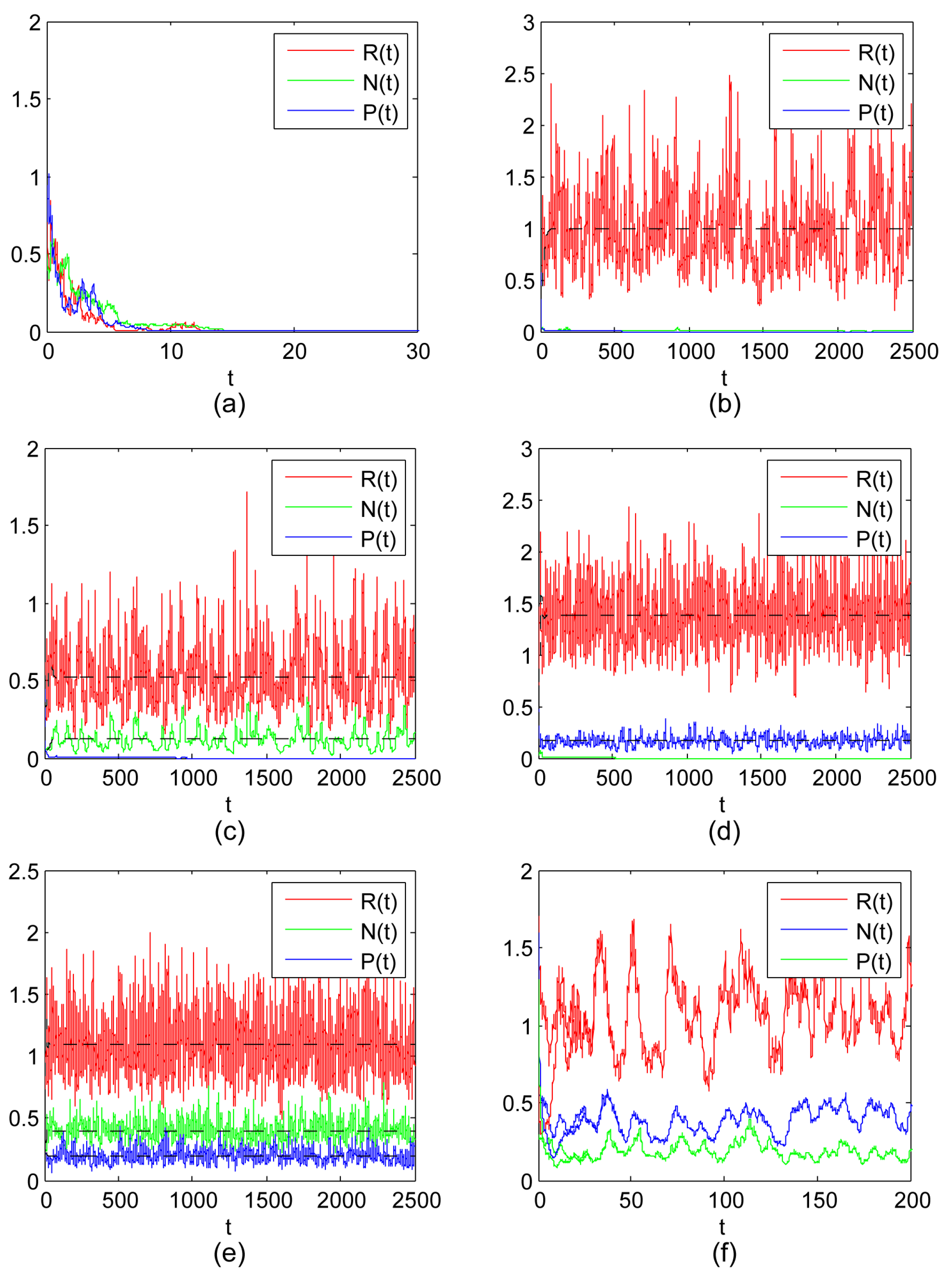
• The existence of both the shared prey and IG prey with the extinction of IG predators, and the existence of both the shared prey and IG predators with the extinction of IG prey are both possible outcomes of the stochastic model (3) with different sets of parameters (see Figure 1c,d). Here, it is worth noting that the noise has a negative effect for IG prey and IG predators, and may also have a positive effect for the shared prey if the values of ${\alpha }_n$ and ${\alpha }_p$ grow larger (see (iii) and (iv) of Theorem 8). This also implies that stochastic fluctuation of N or P would help R to grow larger;
• This study suggests that the shared prey, IG prey and IG predators can coexist together for the stochastic model (3), which implies that it is possible for the coexistence of three species under the influence of environmental noise (see Figure 1e). There is recognition that the noise may be favorable to three-species coexistence if $M_i<0$, $i=1,2,3$ (see (v) of Theorem 8). In addition, we also prove that three-species is stable coexistence for the influence of environmental noise (see Theorem 10 and Figure 1f);
• The study of Theorem 11 suggests that the time average of the population size of model (3) with the development of time is equal to the stationary distribution in space.

References

- Holt, R.D.; Polis, G.A. A theoretical framework for intraguild predation. Am. Nat. 1997, 149, 745–764. [Google Scholar] [CrossRef]
- Polis, G.A.; Holt, R.D. Intraguild predation: The dynamics of complex trophic interactions. Trends Ecol. Evol. 1992, 7, 151–154. [Google Scholar] [CrossRef]
- Hsu, S.B.; Ruan, S.G.; Yang, T.H. Analysis of three species Lotka–Volterra food web models with omnivory. J. Math. Anal. Appl. 2015, 426, 659–687. [Google Scholar] [CrossRef]
- Shchekinova, E.Y.; Löder, M.G.J.; Boersma, M.; Wiltshire, K.H. Facilitation of intraguild prey by its intraguild predator in a three-species Lotka–Volterra model. Theor. Popul. Biol. 2014, 92, 55–61. [Google Scholar] [CrossRef] [PubMed]
- Velazquez, I.; Kaplan, D.; Velasco-Hernandez, J.X.; Navarrete, S.A. Multistability in an open recruitment food web model. Appl. Math. Comput. 2005, 163, 275–294. [Google Scholar] [CrossRef]
- Abrams, P.A.; Fung, S.R. Prey persistence and abundance in systems with intraguild predation and type-2 functional responses. J. Theor. Biol. 2010, 264, 1033–1042. [Google Scholar] [CrossRef] [PubMed]
- Freeze, M.; Chang, Y.; Feng, W. Analysis of dynamics in a complex food chain with ratio-dependent functional response. J. Appl. Anal. Comput. 2014, 4, 69–87. [Google Scholar]
- Verdy, A.; Amarasekare, P. Alternative stable states in communities with intraguild predation. J. Theor. Biol. 2010, 262, 116–128. [Google Scholar] [CrossRef] [PubMed]
- Urbani, P.; Ramos-Jiliberto, R. Adaptive prey behavior and the dynamics of intraguild predation systems. Ecol. Model. 2010, 221, 2628–2633. [Google Scholar] [CrossRef]
- Zabalo, J. Permanence in an intraguild predation model with prey switching. Bull. Math. Biol. 2012, 74, 1957–1984. [Google Scholar] [CrossRef] [PubMed]
- Fan, M.; Kuang, Y.; Feng, Z.L. Cats protecting birds revisited. Bull. Math. Biol. 2005, 67, 1081–1106. [Google Scholar] [CrossRef] [PubMed]
- Kang, Y.; Wedekin, L. Dynamics of a intraguild predation model with generalist or specialist predator. J. Math. Biol. 2013, 67, 1227–1259. [Google Scholar] [CrossRef] [PubMed]
- Shu, H.Y.; Hu, X.; Wang, L.; Watmough, J. Delay induced stability switch, multitype bistability and chaos in an intraguild predation model. J. Math. Biol. 2015, 71, 1269–1298. [Google Scholar] [CrossRef] [PubMed]
- Golec, J.; Sathananthan, S. Stability analysis of a stochastic logistic model. Math. Comput. Model. 2003, 38, 585–593. [Google Scholar] [CrossRef]
- Jiang, D.Q.; Shi, N.Z.; Li, X.Y. Global stability and stochastic permanence of a non-autonomous logistic equation with random perturbation. J. Math. Anal. Appl. 2008, 340, 588–597. [Google Scholar] [CrossRef]
- Liu, M.; Wang, K.; Hong, Q. Stability of a stochastic logistic model with distributed delay. Math. Comput. Model. 2013, 57, 1112–1121. [Google Scholar] [CrossRef]
- Aguirre, P.; González-Olivares, E.; Torres, S. Stochastic predator–prey model with Allee effect on prey. Nonlinear Anal. RWA 2013, 14, 768–779. [Google Scholar] [CrossRef]
- Ji, C.Y.; Jiang, D.Q. Dynamics of a stochastic density dependent predator–prey system with Beddington-DeAngelis functional response. J. Math. Anal. Appl. 2011, 381, 441–453. [Google Scholar] [CrossRef]
- Liu, M.; Wang, K. Global stability of a nonlinear stochastic predator–prey system with Beddington-DeAngelis functional response. Commun. Nonlinear Sci. 2011, 16, 1114–1121. [Google Scholar] [CrossRef]
- Mandal, P.S.; Banerjee, M. Stochastic persistence and stability analysis of a modified Holling-Tanner model. Math. Method. Appl. Sci. 2013, 36, 1263–1280. [Google Scholar] [CrossRef]
- Saha, T.; Chakrabarti, C. Stochastic analysis of prey-predator model with stage structure for prey. J. Appl. Math. Comput. 2011, 35, 195–209. [Google Scholar] [CrossRef]
- Vasilova, M. Asymptotic behavior of a stochastic Gilpin-Ayala predator–prey system with time-dependent delay. Math. Comput. Model. 2013, 57, 764–781. [Google Scholar] [CrossRef]
- Yagi, A.; Ton, T.V. Dynamic of a stochastic predator–prey population. Appl. Math. Comput. 2011, 218, 3100–3109. [Google Scholar] [CrossRef]
- Jovanović, M.; Vasilova, M. Dynamics of non-autonomous stochastic Gilpin-Ayala competition model with time-varying delays. Appl. Math. Comput. 2013, 219, 6946–6964. [Google Scholar] [CrossRef]
- Li, X.; Mao, X. Population dynamical behavior of non-autonomous Lotka–Volterra competitive system with random perturbation. Discrete Cont. Dyn. Syst. Ser. 2009, 24, 523–593. [Google Scholar]
- Lian, B.S.; Hu, S.G. Asymptotic behaviour of the stochastic Gilpin-Ayala competition models. J. Math. Anal. Appl. 2008, 339, 419–428. [Google Scholar] [CrossRef]
- Zhu, C.; Yin, G. On competitive Lotka–Volterra model in random environments. J. Math. Anal. Appl. 2009, 357, 154–170. [Google Scholar] [CrossRef]
- Ji, C.Y.; Jiang, D.Q.; Liu, H.; Yang, Q.S. Existence, uniqueness and ergodicity of positive solution of mutualism system with stochastic perturbation. Math. Probl. Eng. 2010, 2010. [Google Scholar] [CrossRef]
- Liu, M.; Wang, K. Analysis of a stochastic autonomous mutualism model. J. Math. Anal. Appl. 2013, 402, 392–403. [Google Scholar] [CrossRef]
- Liu, M.; Wang, K. Population dynamical behavior of Lotka–Volterra cooperative systems with random perturbations. Discrete Cont. Dyn. Syst. Ser. 2013, 33, 2495–2522. [Google Scholar] [CrossRef]
- Liu, Q. Analysis of a stochastic non-autonomous food-limited Lotka–Volterra cooperative model. Appl. Math. Comput. 2015, 254, 1–8. [Google Scholar] [CrossRef]
- Liu, M.; Wang, K. Dynamics of a two-prey one-predator system in random environments. J. Nonlinear Sci. 2013, 23, 751–775. [Google Scholar] [CrossRef]
- May, R.M. Stability and Complexity in Model Ecosystems; Princeton University Press: Princeton, NJ, USA, 1973. [Google Scholar]
- Has’minskii, R.Z. Stochastic Stability of Differential Equations; Sijthoff & Noordhoff: Alphen aan den Rijn, the Netherlands, 1980. [Google Scholar]
- Karatzas, I.; Shreve, S. Brownian Motion and Stochastic Calculus; Springer: Berlin, Germany, 1991. [Google Scholar]
- Barbalat, I. Systems d’equations differentielles d’oscillations nonlineaires. Rev. Roum. Math. Pures Appl. 1959, 4, 267–270. [Google Scholar]
- Gard, T.C. Introduction to Stochastic Differential Equations; Marcel Dekker, Inc.: New York, NY, USA, 1988. [Google Scholar]
- Strang, G. Linear Algebra and Its Applications; Wellesley-Cambridge Press: London, UK, 1988. [Google Scholar]
- Zhu, C.; Yin, G. Asymptotic properties of hybrid diffusion systems. SIAM J. Control Optim. 2007, 46, 1155–1179. [Google Scholar] [CrossRef]
© 2016 by the authors; licensee MDPI, Basel, Switzerland. This article is an open access article distributed under the terms and conditions of the Creative Commons Attribution (CC-BY) license (http://creativecommons.org/licenses/by/4.0/).