
An Efficient Approach for Fast and Accurate Voltage Stability Margin Computation in Large Power Grids

Abstract
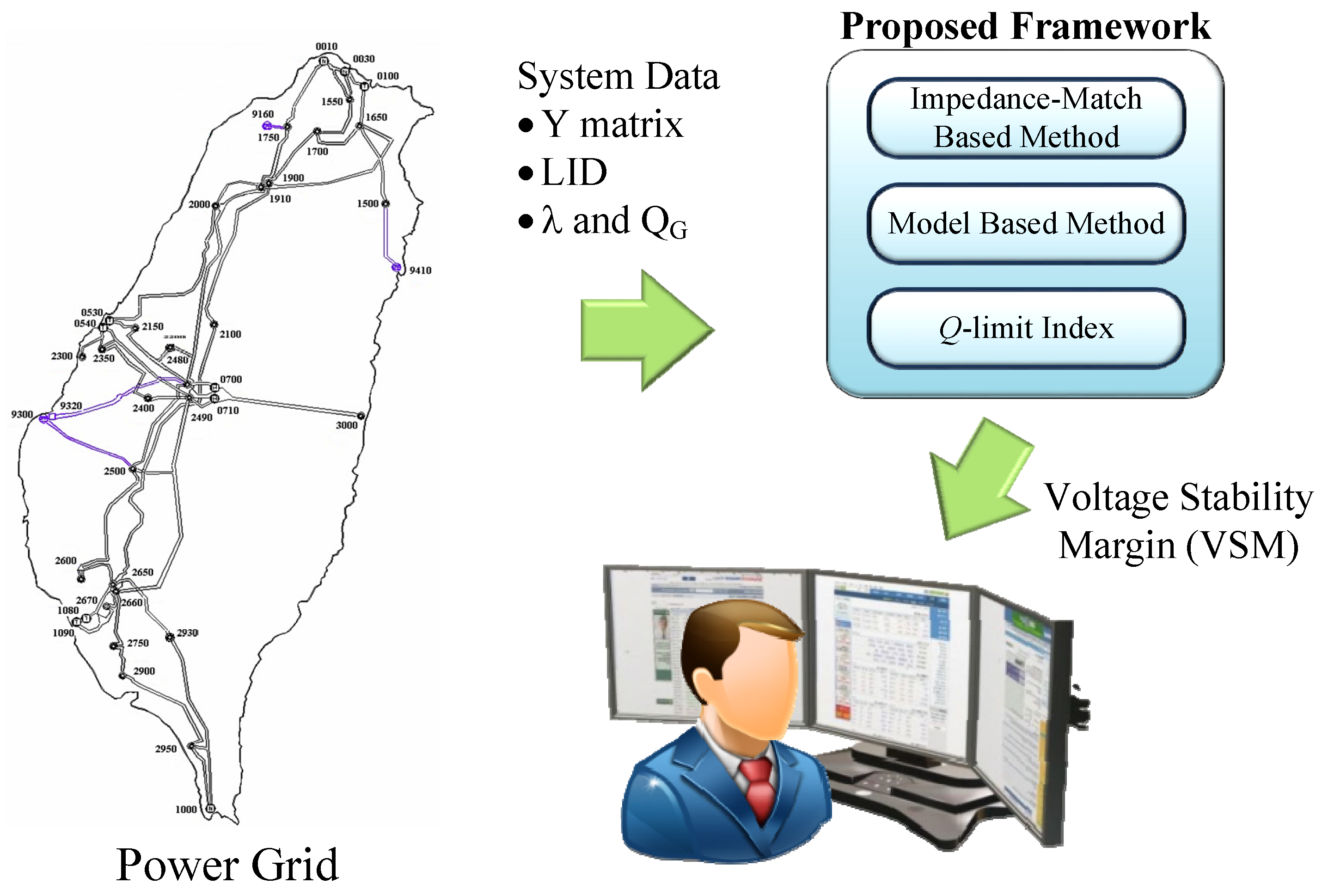
:1. Introduction
2. Proposed Approach
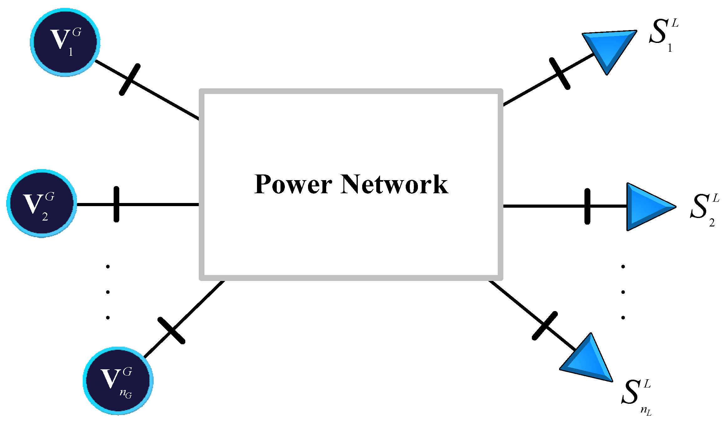
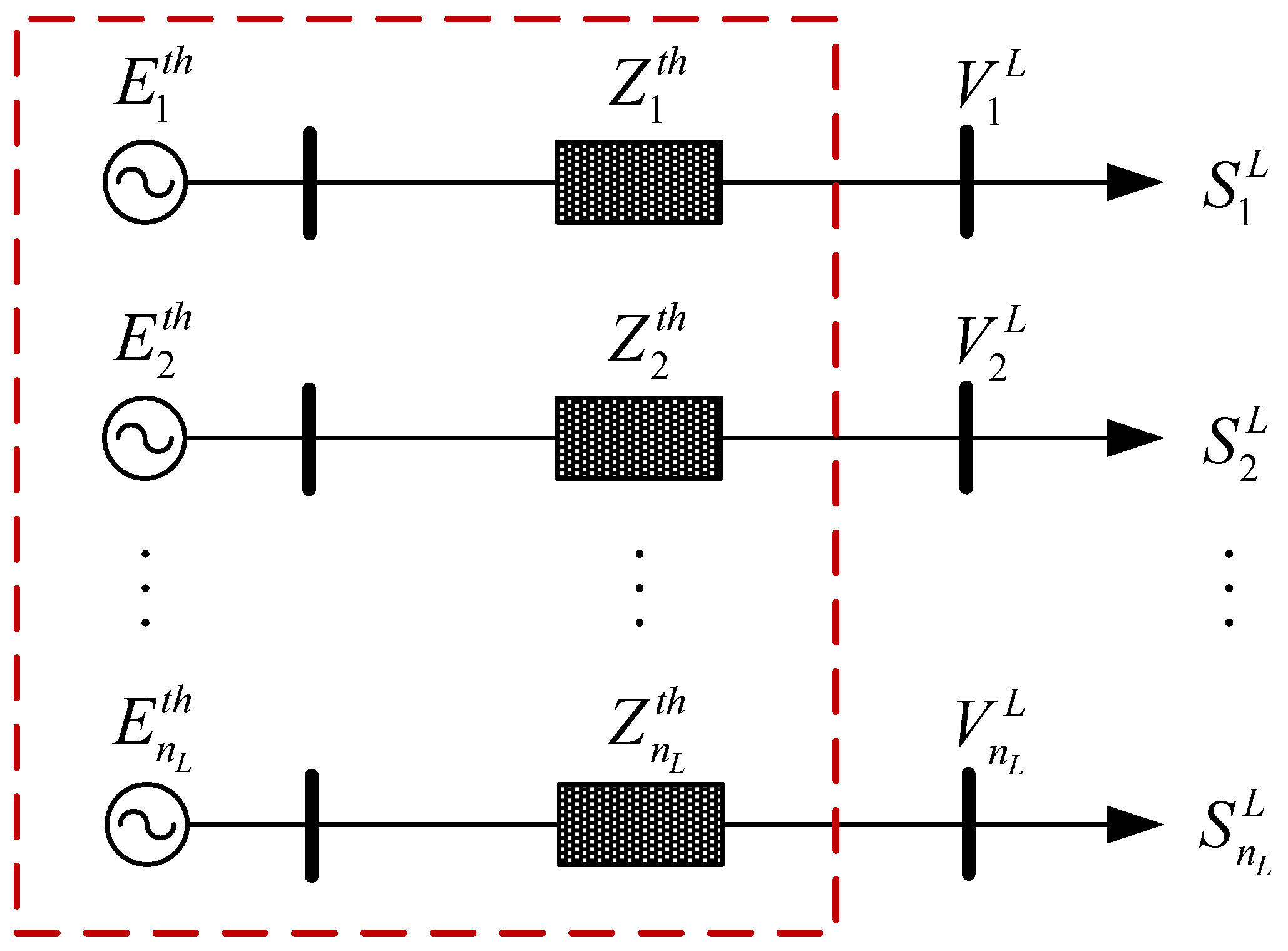
2.1. Multi-Node Thevenin Equivalent Circuit Model
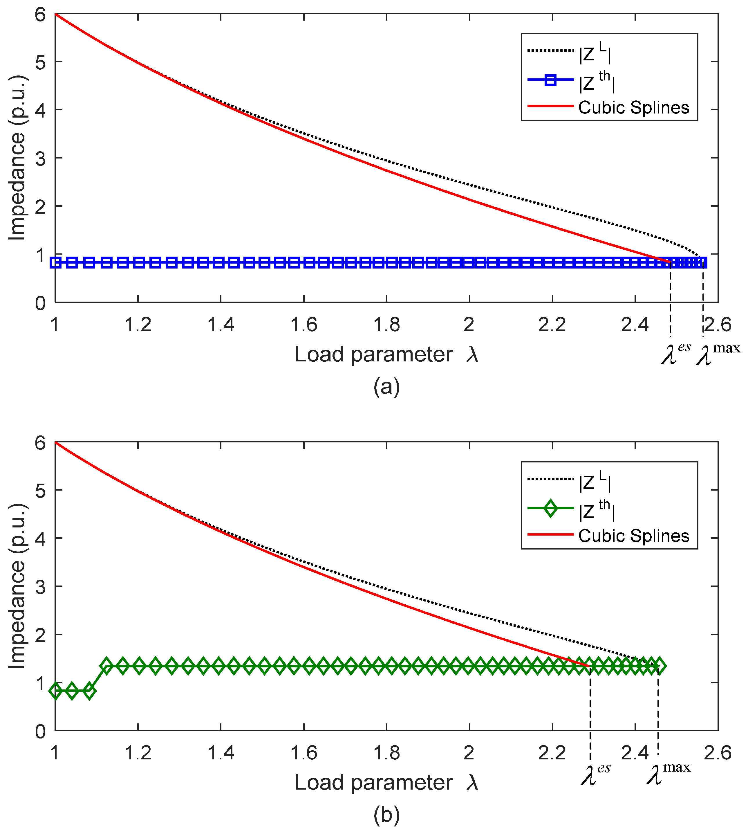
2.2. Cubic Spline Extrapolation Technique
2.3. Generator Q-Limit Index
| Algorithm 1. Identify generator Q limit violations. |
| Input: for and LID; 1: function Qlimit(D) 2: Find by solving ; 3: ; 4: if or then 5: Bus type change for bus i (PV bus to PQ bus); 6: end if 7: return List of Q limit violations 8: end function |
2.4. Continuation Technique
- (1)
- Compute for to create a list of Q limit violations ;
- (2)
- Employ a multi-node Thevenin equivalent network to model a power system. Next, calculate and for based on ;
- (3)
- Utilize cubic spline extrapolation technique to estimate based on and ;
- (4)
- Execute a continuation program to determine the exact through the information of ;
- (5)
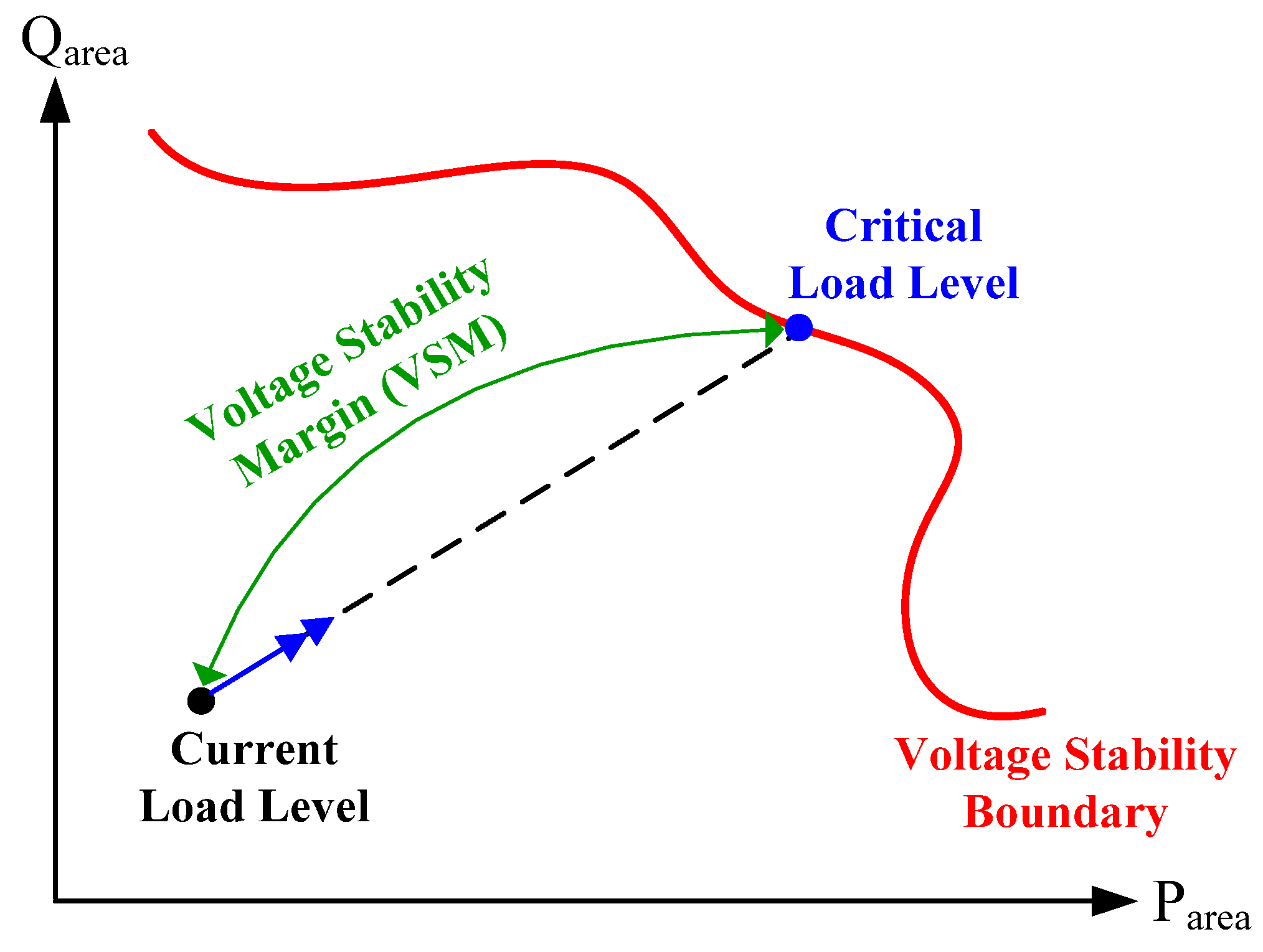
- Compute VSM via Equation (12).
| Algorithm 2. Determine VSM via the proposed method. |
| 1: Input: , three sets of , , and ; 2: ; 3: for do 4: Qlimit(D); 5: end for 6: Compute Z by Equation (4) based on ; 7: Compute for by Equation (8); 8: Estimate via cubic spline extrapolation technique; 9: Determine based on via a continuation program; 10: Compute VSM by Equation (12); 11: return VSM |
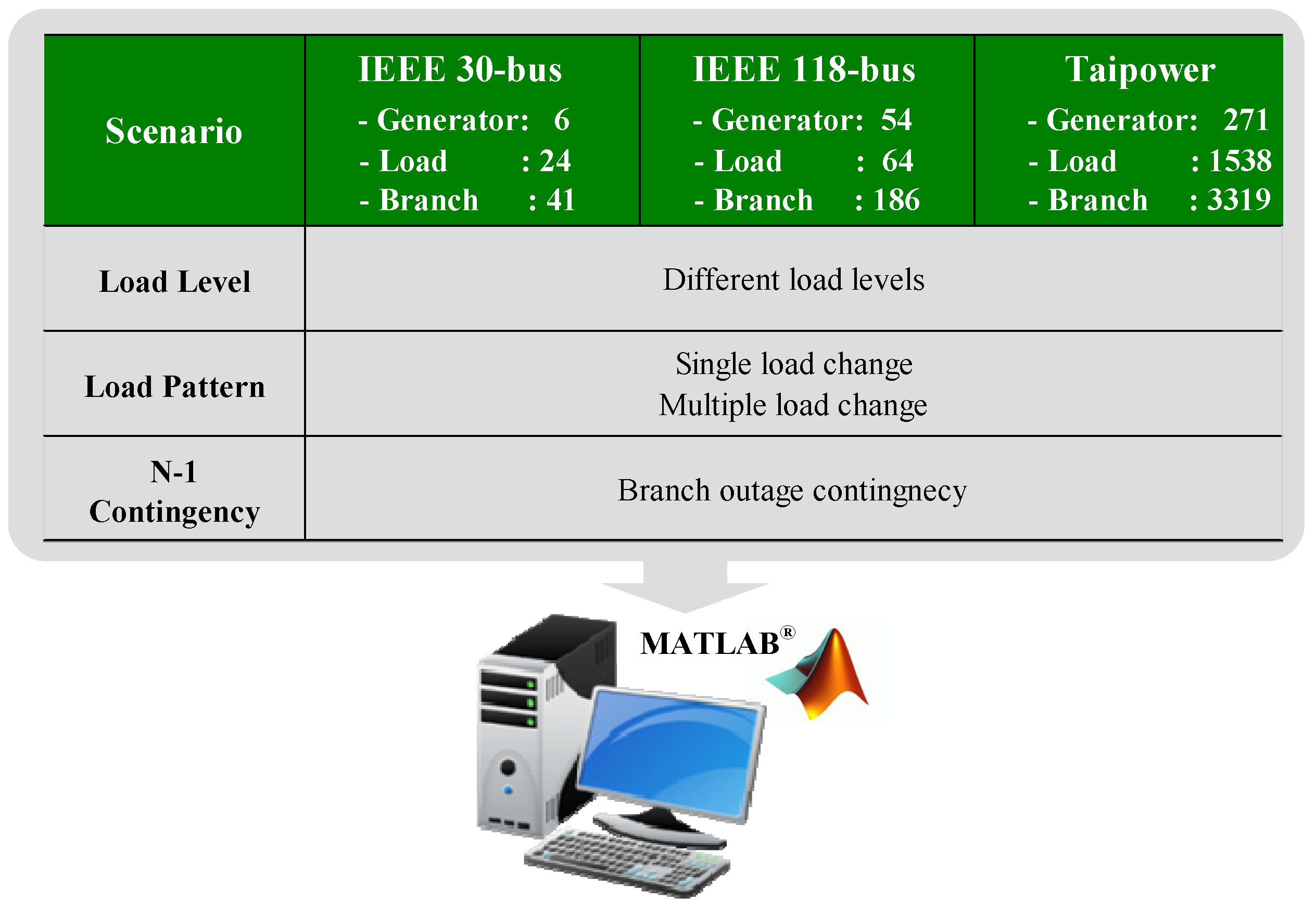
3. Simulation Results
3.1. Effects of Different Load Increase Scenarios
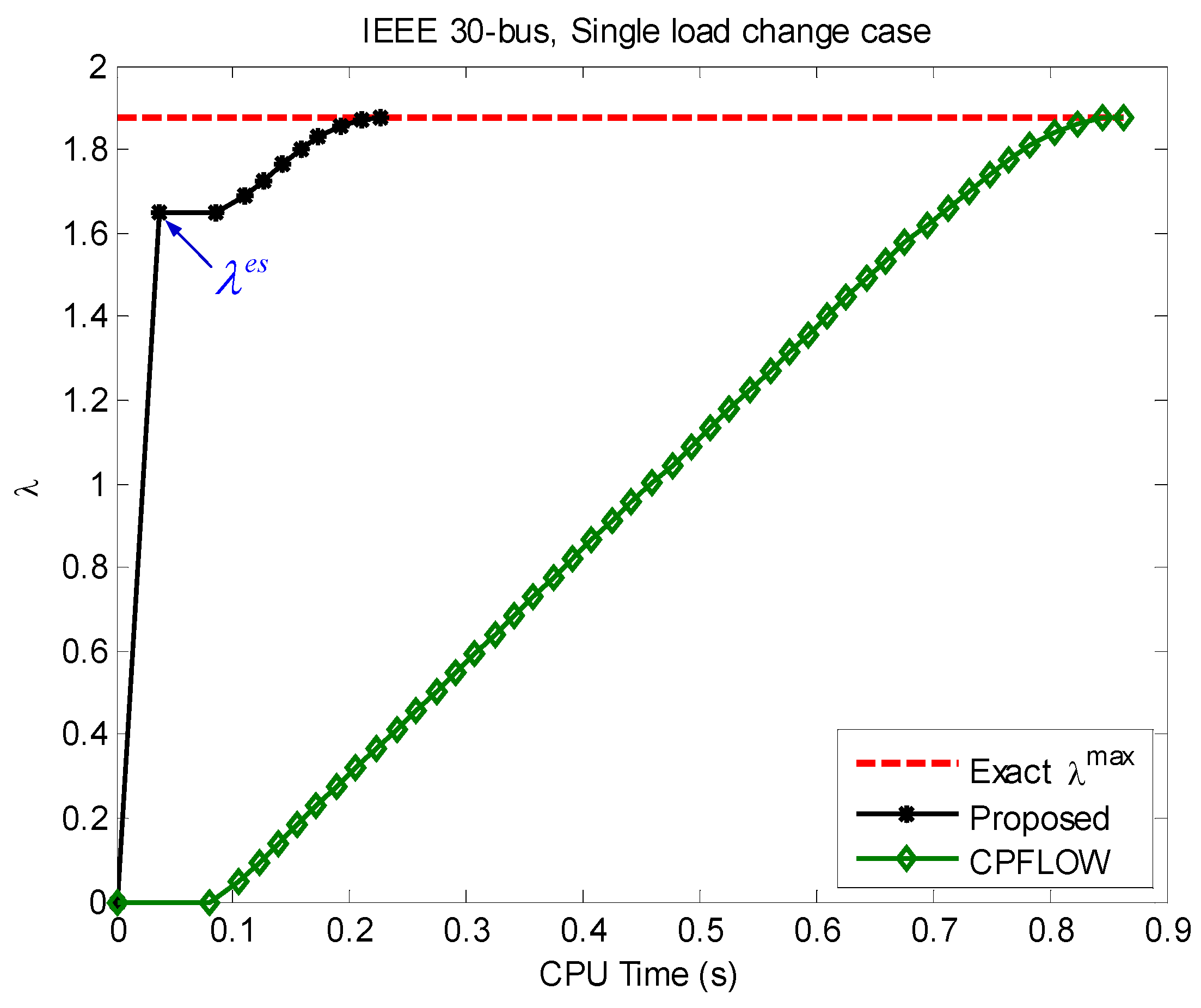
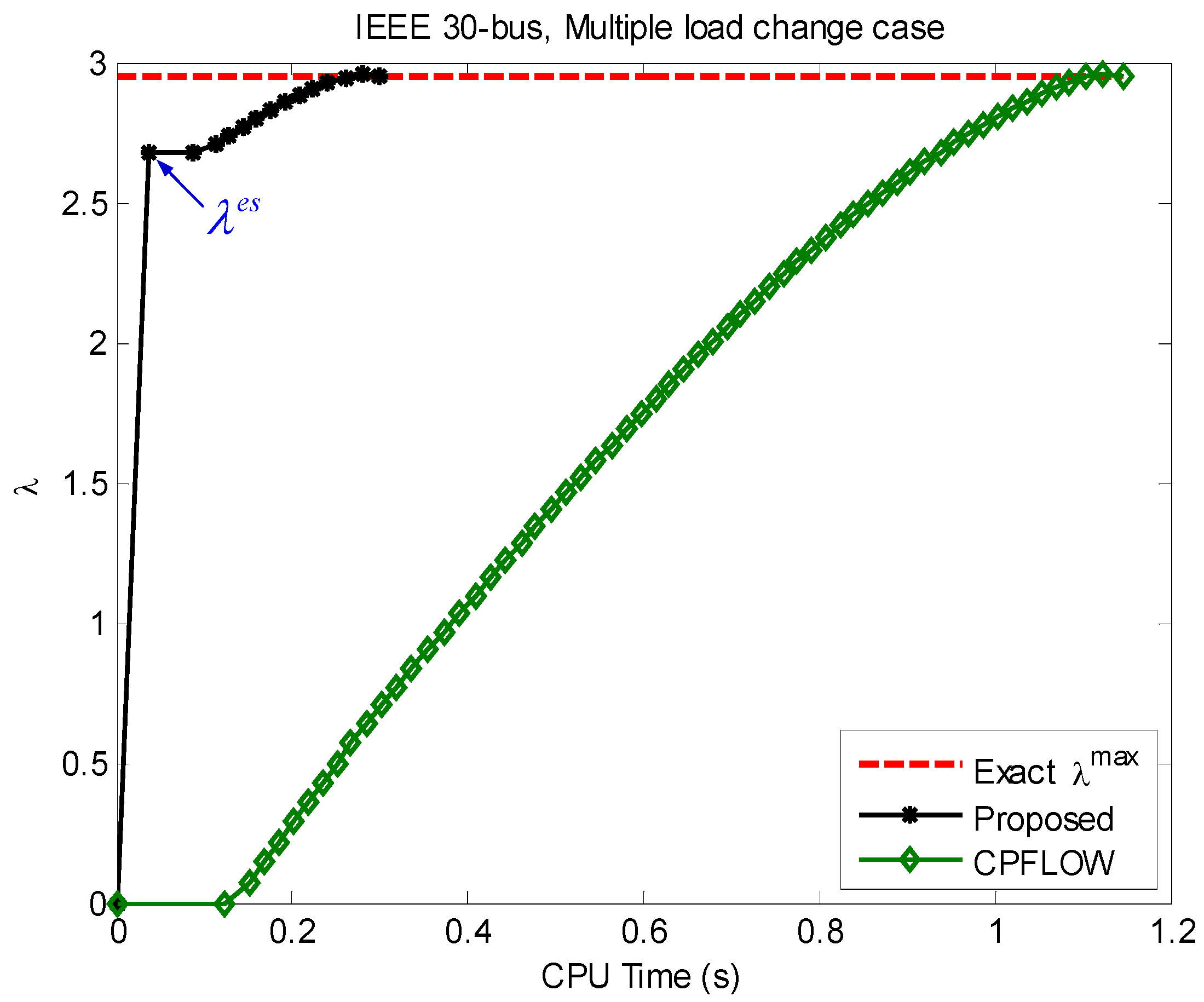
3.1.1. IEEE 30-Bus System
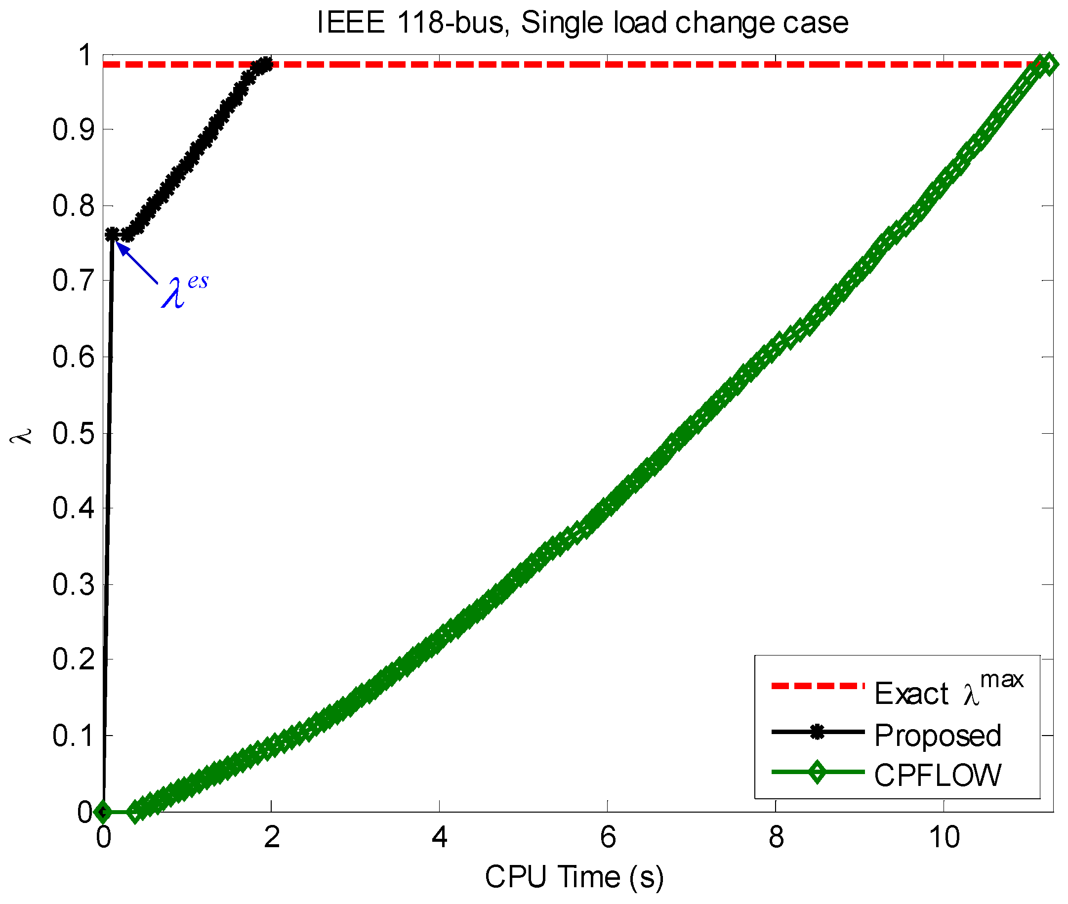
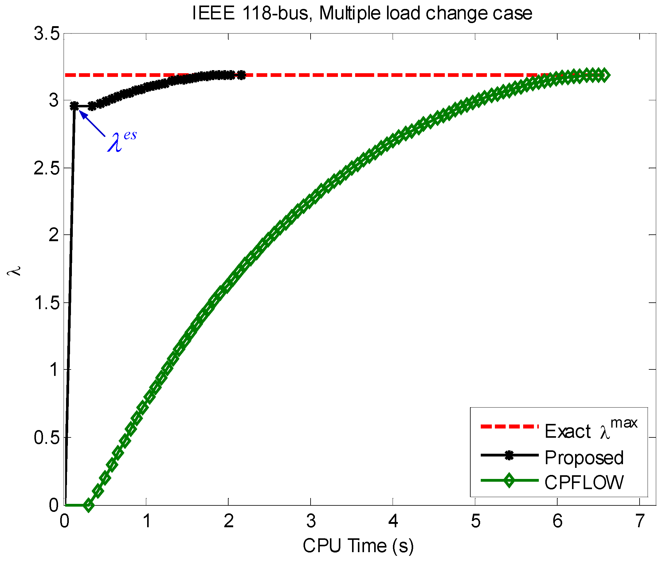
3.1.2. IEEE 118-Bus System
3.2. Effects of Q Limits Violation
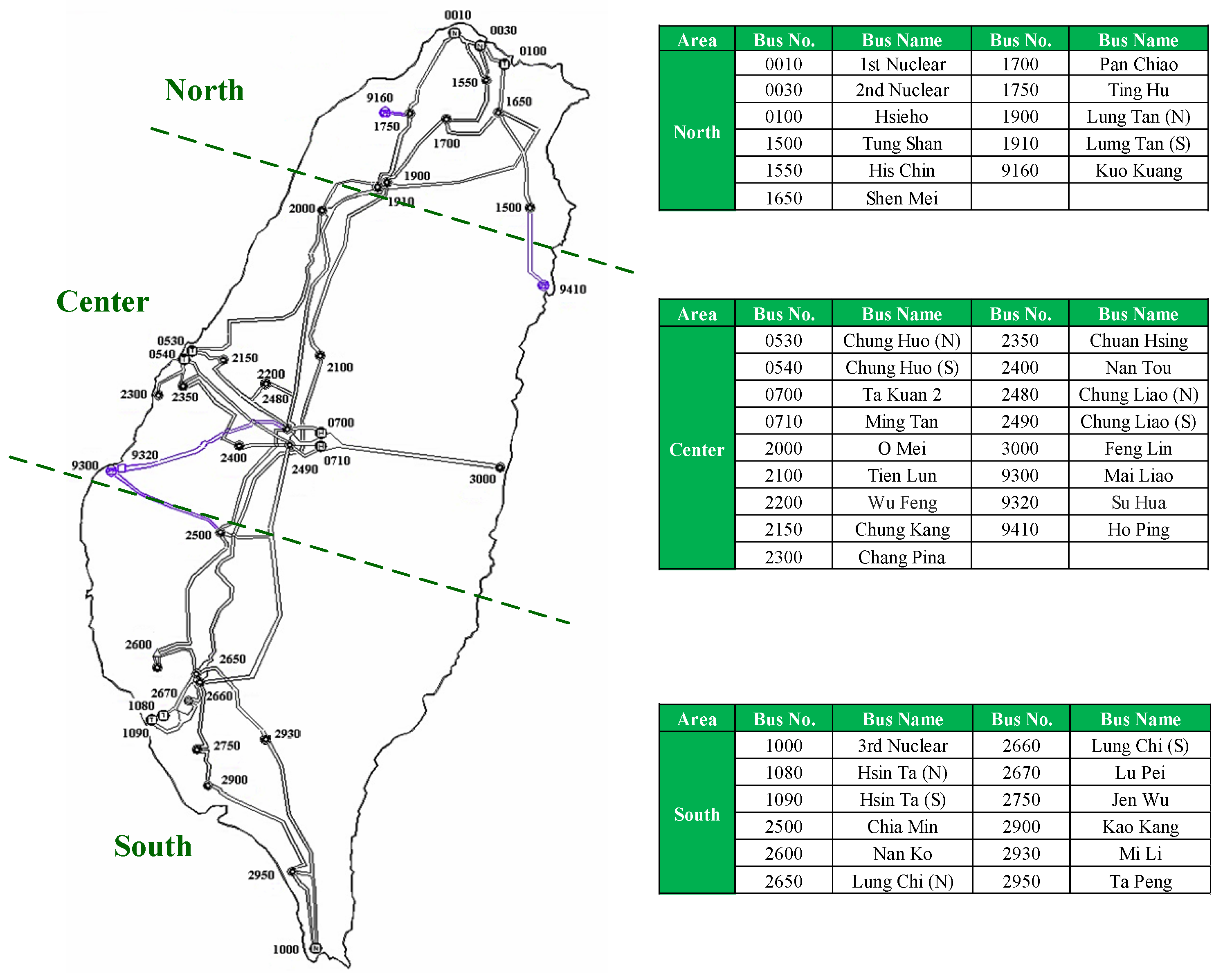
3.3. Taiwan Power (Taipower) System
3.4. Statistical Evalution
3.5. N-1 Contingency Analysis
3.6. Comparison with Machine Learning Tools
3.7. Comparison with Line Voltage Stability Index
4. Conclusions
Acknowledgments
Conflicts of Interest
References
- Kundur, P. Power System Stability and Control; McGraw-Hill: New York, NY, USA, 1994. [Google Scholar]
- Taylor, C.W. Power System Voltage Stability; McGraw-Hill: New York, NY, USA, 1994. [Google Scholar]
- Su, H.Y.; Chen, Y.C.; Hsu, Y.L. A synchrophasor based optimal voltage control scheme with successive voltage stability margin improvement. Appl. Sci. 2016, 6, 1–12. [Google Scholar] [CrossRef]
- Kundur, P.; Paserba, J.; Ajjarapu, V.; Andersson, G.; Bose, A.; Canizares, C.; Hatziargyriou, N.; Hill, D.; Stankovic, A.; Taylor, C.; et al. Definition and classification of power system stability IEEE/CIGRE joint task force on stability terms and definitions. IEEE Trans. Power Syst. 2004, 19, 1387–1401. [Google Scholar]
- Morison, G.K.; Gao, B.; Kundur, P. Voltage stability analysis using static and dynamic approaches. IEEE Trans. Power Syst. 1993, 8, 1159–1171. [Google Scholar] [CrossRef]
- Andersson, G.; Donalek, P.; Farmer, R.; Hatziargyriou, N.; Kamwa, I.; Kundur, P.; Martins, N.; Paserba, J.; Pourbeik, P.; Sanchez-Gasca, J.; et al. Causes of the 2003 major grid blackouts in north America and Europe, and recommended means to improve system dynamic performance. IEEE Trans. Power Syst. 2005, 20, 1922–1928. [Google Scholar] [CrossRef]
- Ajjarapu, V. Computational Techniques for Voltage Stability Assessment and Control; Springer: New York, NY, USA, 2006. [Google Scholar]
- Simpson-Porco, J.W.; Dörfler, F.; Bullo, F. Voltage collapse in complex power grids. Nat. Commun. 2016. [Google Scholar] [CrossRef] [PubMed]
- Begovic, M.; Fulton, D.; Gonzalez, M.R. Summary of system protection and voltage stability. IEEE Trans. Power Del. 1995, 10, 631–638. [Google Scholar] [CrossRef]
- Schlueter, R.A. A voltage stability security assessment method. IEEE Trans. Power Syst. 1998, 13, 1423–1438. [Google Scholar] [CrossRef]
- Flatabo, N.; Ognedal, R.; Carlsen, T. Voltage stability condition in a power transmission system calculated by sensitivity methods. IEEE Trans. Power Syst. 1990, 5, 1286–1293. [Google Scholar] [CrossRef]
- Flatabo, N.; Fosso, O.; Ognedal, R.; Carlsen, T. A method for calculation of margins to voltage instability applied on the Norwegian system for maintaining required security level. IEEE Trans. Power Syst. 1993, 8, 920–928. [Google Scholar] [CrossRef]
- Tiranuchit, A.; Thomas, R.J. A posturing strategy against voltage instabilities in electric power systems. IEEE Trans. Power Syst. 1988, 3, 87–93. [Google Scholar] [CrossRef]
- Gao, B.; Morison, G.K.; Kundur, P. Voltage stability evaluation using modal analysis. IEEE Trans. Power Syst. 1992, 7, 1529–1542. [Google Scholar] [CrossRef]
- Zhou, D.Q.; Annakkage, U.D.; Rajapakse, A.D. Online monitoring of voltage stability margin using an artificial neural network. IEEE Trans. Power Syst. 2010, 25, 1566–1574. [Google Scholar] [CrossRef]
- Zheng, C.; Malbasa, V.; Kezunovic, M. Regression tree for stability margin prediction using synchrophasor measurements. IEEE Trans. Power Syst. 2013, 28, 1978–1987. [Google Scholar] [CrossRef]
- Vu, K.; Begovic, M.M.; Novosel, D.; Saha, M.M. Use of local measurements to estimate voltage-stability margin. IEEE Trans. Power Syst. 1999, 14, 1029–1035. [Google Scholar] [CrossRef]
- Smon, I.; Verbic, G.; Gubina, F. Local voltage-stability index using Tllegen’s theorem. IEEE Trans. Power Syst. 2006, 21, 1267–1275. [Google Scholar] [CrossRef]
- Corsi, S.; Taranto, G.N. A real-time voltage instability identification algorithm based on local phasor measurements. IEEE Trans. Power Syst. 2008, 23, 1271–1279. [Google Scholar] [CrossRef]
- Su, H.Y.; Liu, C.W. Estimating the voltage stability margin using PMU measurements. IEEE Trans. Power Syst. 2016, 31, 3221–3229. [Google Scholar] [CrossRef]
- Iba, K.; Suzuli, H.; Egawa, M.; Watanabe, T. Calculation of the critical loading with nose curve using homotopy continuation method. IEEE Trans. Power Syst. 1991, 6, 584–593. [Google Scholar] [CrossRef]
- Ajjarapu, V.; Christy, C. The continuation power flow: A tool for steady state voltage stability analysis. IEEE Trans. Power Syst. 1992, 7, 416–423. [Google Scholar] [CrossRef]
- Canizares, C.A.; Alvarado, F.L. Point of collapse and continuation methods for large AC/DC systems. IEEE Trans. Power Syst. 1993, 8, 1–8. [Google Scholar] [CrossRef]
- Chiang, H.D.; Flueck, A.J.; Shah, K.S.; Balu, N. CPFLOW: A practical tool for tracing power system steady-state stationary behavior due to load and generation variations. IEEE Trans. Power Syst. 1995, 10, 623–634. [Google Scholar] [CrossRef]
- Moghavvemi, M. New method for indicating voltage stability in power system. In Proceedings of the IEEE International Conference on Power Engineering, Singapore, 22–24 May 1997; pp. 223–227.
- Moghavvemi, M.; Faruque, O. Real-time contingency evaluation and ranking technique. IEE Proc.-Gener. Transm. Distrib. 1998, 5, 517–524. [Google Scholar] [CrossRef]
- Cupelli, M.; Doig Cardet, C.; Monti, A. Comparison of line voltage stability indices using dynamic real time simulation. In Proceedings of the 3rd IEEE PES International Conference and Exhibition on Innovative Smart Grid Technologies (ISGT Europe), Berlin, Germany, 14–17 October 2012; pp. 1–8.
- Cupelli, M.; Doig Cardet, C.; Monti, A. Voltage stability indices comparison on the IEEE-39 bus system using RTDS. In Proceedings of the IEEE International Conference on Power System Technology (POWERCON), Auckland, New Zealand, 30 October–2 November 2012; pp. 1–6.
- De Boor, C. A Practical Guide to Splines; Springer: New York, NY, USA, 1978. [Google Scholar]
- Mathworks, Inc., Mathworks Matlab. Available online: http://www.mathworks.com/ (accessed on 4 March 2016).
- Power Systems Test Case Archive, University of Washington College of Engineering. Available online: http://www.ee.washington.edu/re-serach/pstcal/ (accessed on 4 March2016).


| Case | Load Pattern 1 | Q Limit 2 |
|---|---|---|
| 1 | Load_All | QG_All |
| 2 | Load_All | QG_Odd |
| 3 | Load_All | QG_Even |
| 4 | Load_Odd | QG_All |
| 5 | Load_Odd | QG_Odd |
| 6 | Load_Odd | QG_Even |
| 7 | Load_Even | QG_All |
| 8 | Load_Even | QG_Odd |
| 9 | Load_Even | QG_Even |
| 10 | Load_One | QG_All |
| 11 | Load_One | QG_Odd |
| 12 | Load_One | QG_Even |
| Case | VSM (%) | CPU Time (s) | ||||
|---|---|---|---|---|---|---|
| Proposed | CPFLOW | Proposed | CPFLOW | Proposed | CPFLOW | |
| 1 | 2.3328 | 2.3328 | 70.29 | 70.29 | 0.32 | 1.22 |
| 2 | 1.5552 | 1.5552 | 10.11 | 10.11 | 0.39 | 1.28 |
| 3 | 1.8229 | 1.8229 | 28.72 | 28.72 | 0.39 | 1.27 |
| 4 | 2.8577 | 2.8577 | 82.45 | 82.45 | 0.35 | 1.24 |
| 5 | 2.5215 | 2.5215 | 74.97 | 74.97 | 0.38 | 1.29 |
| 6 | 2.3167 | 2.3167 | 51.35 | 51.35 | 0.31 | 1.21 |
| 7 | 1.5116 | 1.5116 | 6.49 | 6.49 | 0.34 | 1.25 |
| 8 | 2.0565 | 2.0565 | 49.95 | 49.95 | 0.38 | 2.14 |
| 9 | 1.6337 | 1.6337 | 20.15 | 20.15 | 0.37 | 1.27 |
| 10 | 2.7236 | 2.7236 | 80.16 | 80.16 | 0.39 | 1.27 |
| 11 | 2.1221 | 2.1221 | 39.98 | 39.98 | 0.36 | 1.22 |
| 12 | 2.0174 | 2.0174 | 37.69 | 37.69 | 0.31 | 1.25 |
| Case | VSM (%) | CPU Time (s) | ||||
|---|---|---|---|---|---|---|
| Proposed | CPFLOW | Proposed | CPFLOW | Proposed | CPFLOW | |
| 1 | 2.6405 | 2.6405 | 38.76 | 38.76 | 2.95 | 11.81 |
| 2 | 3.1871 | 3.1871 | 50.29 | 50.29 | 3.14 | 10.42 |
| 3 | 1.4769 | 1.4769 | 6.31 | 6.31 | 3.21 | 12.45 |
| 4 | 1.5283 | 1.5283 | 14.41 | 14.41 | 3.25 | 10.54 |
| 5 | 2.1263 | 2.1263 | 23.73 | 23.73 | 2.78 | 11.51 |
| 6 | 1.7207 | 1.7207 | 14.81 | 14.81 | 3.18 | 12.25 |
| 7 | 2.8146 | 2.8146 | 48.78 | 48.78 | 3.15 | 12.99 |
| 8 | 2.6706 | 2.6706 | 44.97 | 44.97 | 2.67 | 13.25 |
| 9 | 1.8404 | 1.8404 | 19.92 | 19.92 | 2.63 | 11.67 |
| 10 | 2.6282 | 2.6282 | 32.45 | 32.45 | 2.99 | 10.09 |
| 11 | 2.2282 | 2.2282 | 27.54 | 27.54 | 3.45 | 10.13 |
| 12 | 2.4259 | 2.4259 | 30.15 | 30.15 | 2.84 | 10.55 |
| Case | VSM (%) | CPU Time (s) | ||||
|---|---|---|---|---|---|---|
| Proposed | CPFLOW | Proposed | CPFLOW | Proposed | CPFLOW | |
| 1 | 1.4223 | 1.4223 | 23.16 | 23.16 | 125.36 | 506.22 |
| 2 | 1.3839 | 1.3839 | 18.69 | 18.69 | 118.08 | 510.17 |
| 3 | 1.2641 | 1.2641 | 9.56 | 9.56 | 127.28 | 511.98 |
| 4 | 1.2022 | 1.2022 | 5.87 | 5.87 | 117.89 | 525.42 |
| 5 | 1.3817 | 1.3817 | 17.14 | 17.14 | 128.76 | 523.11 |
| 6 | 1.5732 | 1.5732 | 42.12 | 42.12 | 125.87 | 514.41 |
| 7 | 1.2587 | 1.2587 | 15.68 | 15.68 | 120.22 | 520.35 |
| 8 | 1.4059 | 1.4059 | 22.61 | 22.61 | 129.21 | 526.41 |
| 9 | 1.2831 | 1.2831 | 11.89 | 11.89 | 129.97 | 529.56 |
| 10 | 1.4164 | 1.4164 | 22.48 | 22.48 | 118.79 | 518.15 |
| 11 | 1.5185 | 1.5185 | 38.53 | 38.53 | 130.51 | 530.76 |
| 12 | 1.4611 | 1.4611 | 33.96 | 33.96 | 119.44 | 522.49 |
| Test System | No. of Generators | No. of Loads | No. of Lines | Average CPU Time (s) | |
|---|---|---|---|---|---|
| Proposed | CPFLOW | ||||
| IEEE 30-bus | 6 | 24 | 41 | 0.36 | 1.25 |
| IEEE 118-bus | 54 | 64 | 186 | 3.03 | 11.81 |
| Taipower | 271 | 1538 | 3319 | 121.27 | 502.08 |
| Rank | Branch Outage | CPU Time (s) | ||
|---|---|---|---|---|
| Proposed | CPFLOW | |||
| 1 | 1-2 | 1.2575 | 0.57 | 2.26 |
| 2 | 28-27 | 1.5173 | 0.58 | 2.27 |
| 3 | 27-30 | 2.0271 | 0.55 | 2.24 |
| 4 | 2-5 | 2.2107 | 0.57 | 2.26 |
| 5 | 27-29 | 2.2289 | 0.54 | 2.24 |
| 6 | 9-10 | 2.3951 | 0.58 | 2.27 |
| 7 | 4-12 | 2.4150 | 0.57 | 2.26 |
| 8 | 29-30 | 2.5819 | 0.57 | 2.25 |
| 9 | 12-13 | 2.6331 | 0.57 | 2.26 |
| 10 | 6-8 | 2.6630 | 0.58 | 2.26 |
| 11 | 22-24 | 2.7053 | 0.56 | 2.27 |
| 12 | 12-15 | 2.7439 | 0.57 | 2.26 |
| 13 | 9-11 | 2.7808 | 0.57 | 2.25 |
| 14 | 15-23 | 2.7828 | 0.56 | 2.24 |
| 15 | 6-28 | 2.7883 | 0.56 | 2.24 |
| 16 | 6-9 | 2.7885 | 0.56 | 2.24 |
| 17 | 10-20 | 2.8045 | 0.57 | 2.25 |
| 18 | 2-6 | 2.8076 | 0.56 | 2.23 |
| 19 | 10-21 | 2.8089 | 0.57 | 2.26 |
| 20 | 8-28 | 2.8351 | 0.57 | 2.27 |
| 21 | 24-25 | 2.8471 | 0.55 | 2.23 |
| 22 | 2-4 | 2.8531 | 0.54 | 2.24 |
| 23 | 23-24 | 2.8735 | 0.56 | 2.23 |
| 24 | 6-10 | 2.8750 | 0.58 | 2.27 |
| 25 | 4-6 | 2.8781 | 0.56 | 2.23 |
| 26 | 1-3 | 2.8908 | 0.55 | 2.24 |
| 27 | 3-4 | 2.8989 | 0.56 | 2.26 |
| 28 | 12-16 | 2.9045 | 0.56 | 2.25 |
| 29 | 25-27 | 2.9046 | 0.54 | 2.23 |
| 30 | 19-20 | 2.9116 | 0.55 | 2.24 |
| 31 | 12-14 | 2.9149 | 0.54 | 2.23 |
| 32 | 10-22 | 2.9152 | 0.55 | 2.24 |
| 33 | 5-7 | 2.9207 | 0.55 | 2.24 |
| 34 | 15-18 | 2.9238 | 0.57 | 2.25 |
| 35 | 16-17 | 2.9311 | 0.55 | 2.25 |
| 36 | 18-19 | 2.9324 | 0.55 | 2.23 |
| 37 | 14-15 | 2.9329 | 0.57 | 2.26 |
| 38 | 21-22 | 2.9336 | 0.56 | 2.23 |
| 39 | 10-17 | 2.9357 | 0.57 | 2.26 |
| 40 | 6-7 | 2.9388 | 0.56 | 2.24 |
| Total CPU Time (s) | 22.42 | 89.93 | ||
| Test System | Out of Service | VSM (%) | |
|---|---|---|---|
| IEEE 30-bus | G8 | 1.1638 | 16.38 |
| G13 | 1.2144 | 21.44 | |
| Line 1-2 | 1.2575 | 25.75 | |
| Line 28-27 | 1.5173 | 51.73 | |
| IEEE 118-bus | G10 | 1.2387 | 23.87 |
| G24 | 1.3142 | 31.42 | |
| Line 18-19 | 1.5216 | 52.16 | |
| Line 63-64 | 1.4674 | 46.74 | |
| Taipower | G11 | 1.1136 | 11.36 |
| G42 | 1.1597 | 15.97 | |
| Line 30-100 | 1.3742 | 37.42 | |
| Line 220-223 | 1.2961 | 29.61 |
| Case | VSM (%) | |||
|---|---|---|---|---|
| ANN [15] | RT [16] | Proposed | Actual | |
| 1 | 22.61 | 22.43 | 23.16 | 23.16 |
| 2 | 18.33 | 18.26 | 18.69 | 18.69 |
| 3 | 9.28 | 9.25 | 9.56 | 9.56 |
| Proposed | VCPI [26] | ||||
|---|---|---|---|---|---|
| Rank | Line Outage | Value | Rank | Line Outage | Value |
| 1 | 2480-530 | 1.0775 | 1 | 2480-530 | 0.9439 |
| 2 | 1000-2950 | 1.0826 | 2 | 2950-2930 | 0.8864 |
| 3 | 2950-2930 | 1.1019 | 3 | 1000-2950 | 0.8736 |
| 4 | 2900-2950 | 1.1109 | 4 | 1080-2670 | 0.8548 |
| 5 | 1080-2670 | 1.1163 | 5 | 2900-2950 | 0.8312 |
| 6 | 2750-2660 | 1.1295 | 6 | 2750-2660 | 0.7861 |
| 7 | 2490-2500 | 1.1375 | 7 | 2490-2500 | 0.7345 |
| 8 | 2670-2650 | 1.1493 | 8 | 1080-2660 | 06767 |
| 9 | 2900-2750 | 1.1536 | 9 | 2670-2650 | 0.6553 |
| 10 | 2650-2600 | 1.1654 | 10 | 2900-2750 | 0.5651 |
© 2016 by the author; licensee MDPI, Basel, Switzerland. This article is an open access article distributed under the terms and conditions of the Creative Commons Attribution (CC-BY) license (http://creativecommons.org/licenses/by/4.0/).
Share and Cite
Su, H.-Y. An Efficient Approach for Fast and Accurate Voltage Stability Margin Computation in Large Power Grids. Appl. Sci. 2016, 6, 335. https://doi.org/10.3390/app6110335
Su H-Y. An Efficient Approach for Fast and Accurate Voltage Stability Margin Computation in Large Power Grids. Applied Sciences. 2016; 6(11):335. https://doi.org/10.3390/app6110335
Chicago/Turabian StyleSu, Heng-Yi. 2016. "An Efficient Approach for Fast and Accurate Voltage Stability Margin Computation in Large Power Grids" Applied Sciences 6, no. 11: 335. https://doi.org/10.3390/app6110335
APA StyleSu, H.-Y. (2016). An Efficient Approach for Fast and Accurate Voltage Stability Margin Computation in Large Power Grids. Applied Sciences, 6(11), 335. https://doi.org/10.3390/app6110335