
Quantum Wind Driven Optimization for Unmanned Combat Air Vehicle Path Planning


Abstract
:1. Introduction
2. Mathematical Modeling for UCAV Path Planning
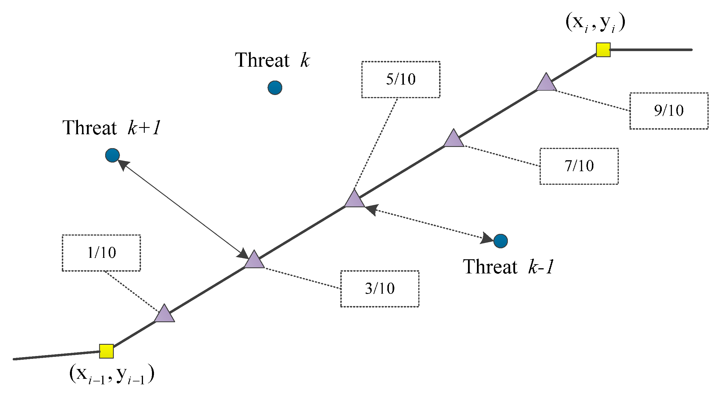
2.1. Threat Resource Model in UCAV Path Planning

2.2. Evaluation Function
3. The Basic Wind Driven Optimization
4. Quantum Computing
5. Quantum Wind Driven Optimization
5.1. Generate Initial Population
5.2. Transformation of the Solution Space
5.3. Updating Process
5.3.1. Updating Formulas of Phase Angle Increment and Phase Angle
5.3.2. Quantum Rotation Gate Strategy
5.3.3. Quantum Non-Gate Strategy
5.4. The Flow Chart of QWDO
| Algorithm 1. Quantum Wind Driven Optimization (QWDO) Algorithm. |
| Step 1. Initialize parameters. N (Population size); G (Max number of generations); RT (RT coefficient); α (The friction coefficient); g (Gravitational constant); c (Constant in the update equation); max V (Maximum allowed speed); Pm (Mutation scale factor). Step 2. Generate Initial Population. Step 3. Transform the solution space according to Equations (23) and (24). Step 4. Evaluate fitness of each air parcel. Step 5. Identify the best solution among all air parcels. Step 6. While stopping criterion is not satisfied
Step 7. End while |
5.5. The Flow Chart of QWDO for UCAV Path Planning
| Algorithm 2. QWDO for UCAV Path Planning Algorithm. |
| Step 1. Initialize parameters. N (Population size); G (Max number of generations); RT (RT coefficient); α (The friction coefficient); g (Gravitational constant); c (Constant in the update equation); Pm (Mutation scale factor). Step 2. Build the UCAV battlefield model. Step 3. Transform coordinate system according to Equation (1). Step 4. Generate Initial Population according to Equation (20). Step 5. Transform the solution space according to Equations (23) and (24). Step 6. Evaluate the cost of each flight path by Equation (5). Step 7. Get the best path. Step 8. While stopping criterion is not satisfied
Step 9. End while |
6. Experimental Results
6.1. Experimental Setup
6.2. Parameters Setting

| Parameters | Value |
|---|---|
| RT coefficient | 1 |
| Constants in the update equation | 0.8 |
| Maximum allowed speed | 0.3 |
| Gravitational constant | 0.6 |
| Coriolis effect | 0.7 |
| The range of phase angle | [−π,π] |
| Parameters | Value |
|---|---|
| Pulse frequency range | [0,2] |
| Maximum pulse emission | 0.5 |
| The maximum loudness | 0.5 |
| Attenuation coefficient of loudness | 0.95 |
| Increasing coefficient of pulse emission | 0.05 |
| The range of phase angle | [−π,π] |
| Parameters | Value |
|---|---|
| Constant inertia | 0.7298 |
| The first acceleration coefficients | 1.4962 |
| The second Acceleration coefficients | 1.4962 |
| The range of phase angle | [−π,π] |
| Parameters | Value |
|---|---|
| RT coefficient | 1 |
| Constants in the update equation | 0.8 |
| Maximum allowed speed | 0.3 |
| Gravitational constant | 0.6 |
| Coriolis effect | 0.7 |
| Parameters | Value |
|---|---|
| Pulse frequency range | [0,2] |
| Maximum pulse emission | 0.5 |
| The maximum loudness | 0.5 |
| Attenuation coefficient of loudness | 0.95 |
| Increasing coefficient of pulse emission | 0.05 |
| Parameters | Value |
|---|---|
| Constant inertia | 0.7298 |
| The first acceleration coefficients | 1.4962 |
| The second Acceleration coefficients | 1.4962 |
| Parameters | Value |
|---|---|
| Mutation scale factor | 0.2 |
| Crossover probability | 0.03 |
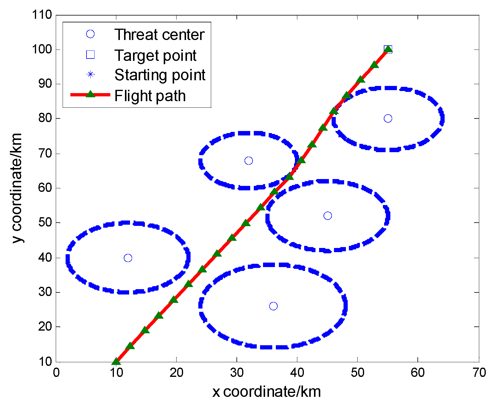
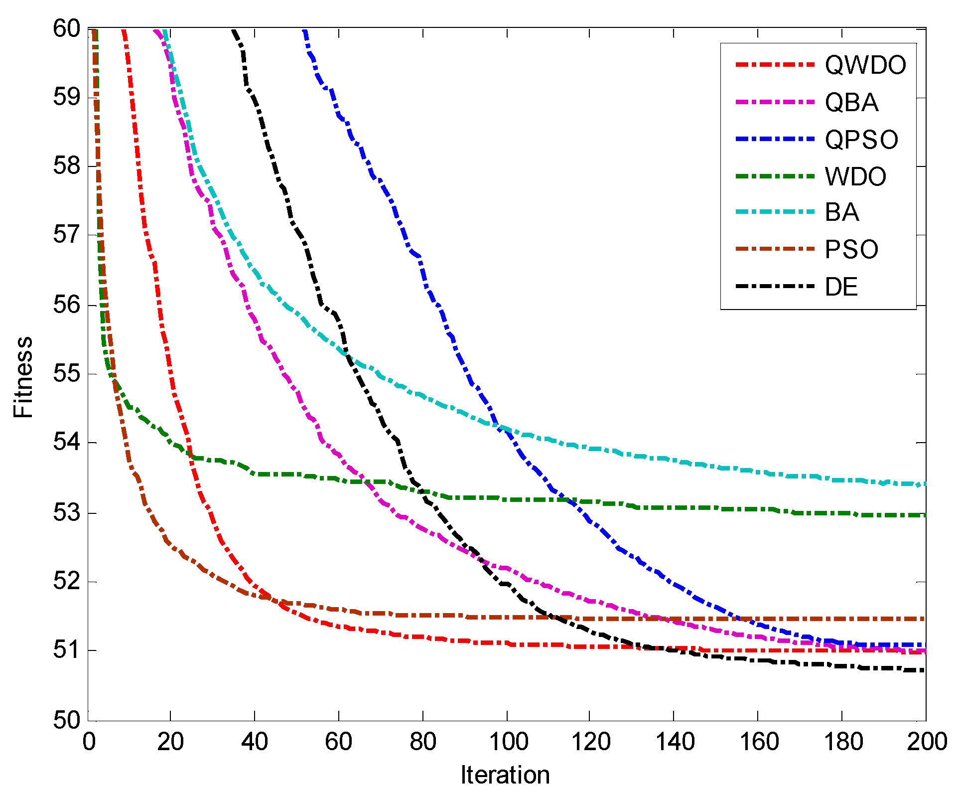
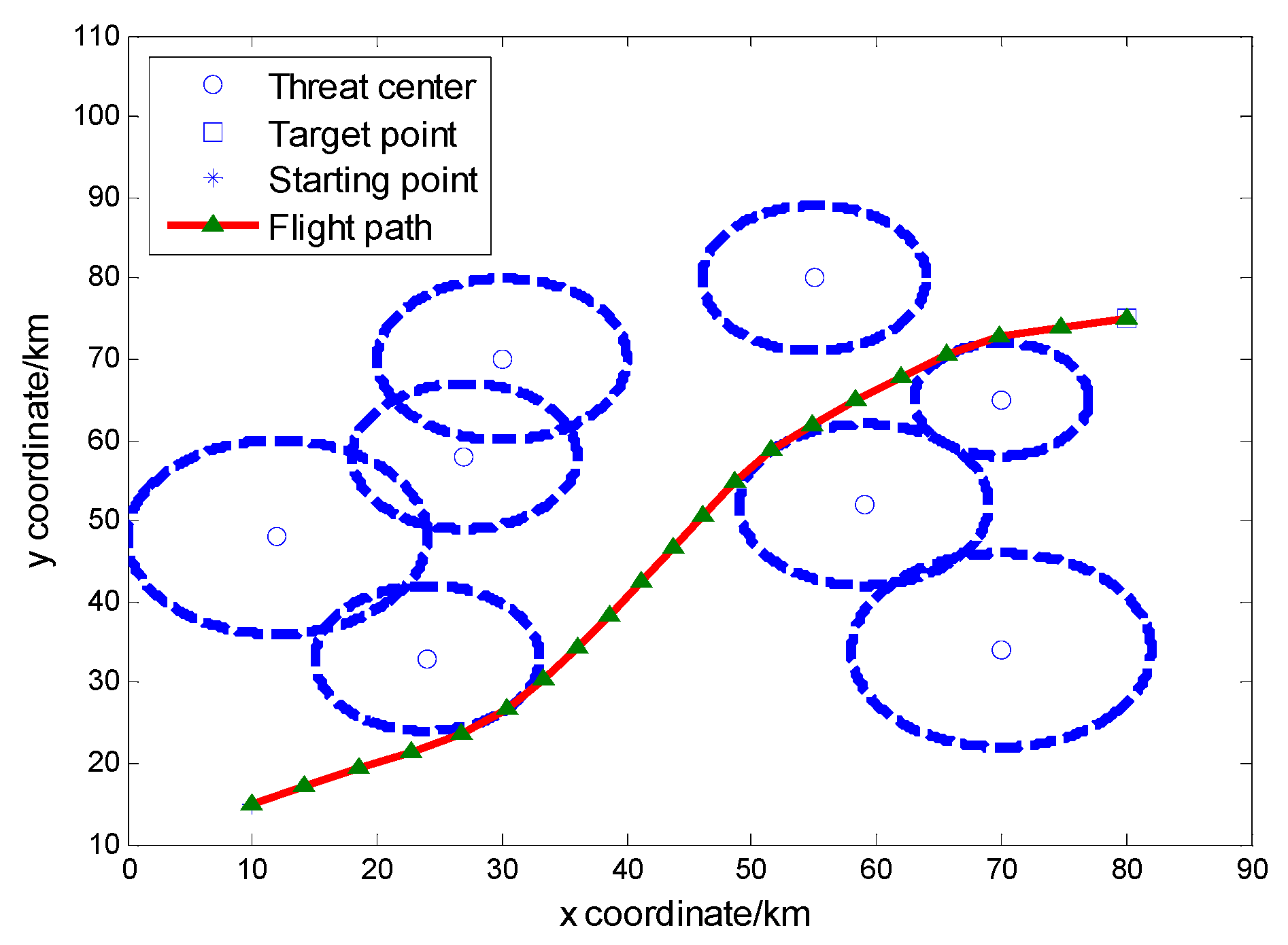
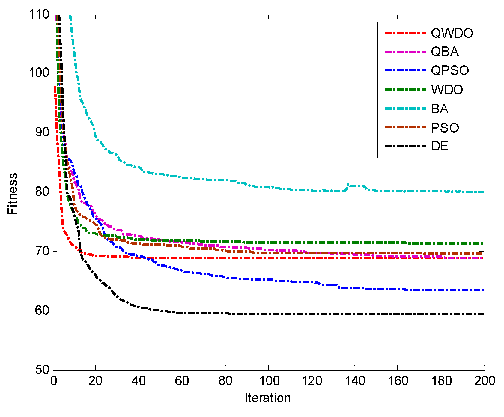
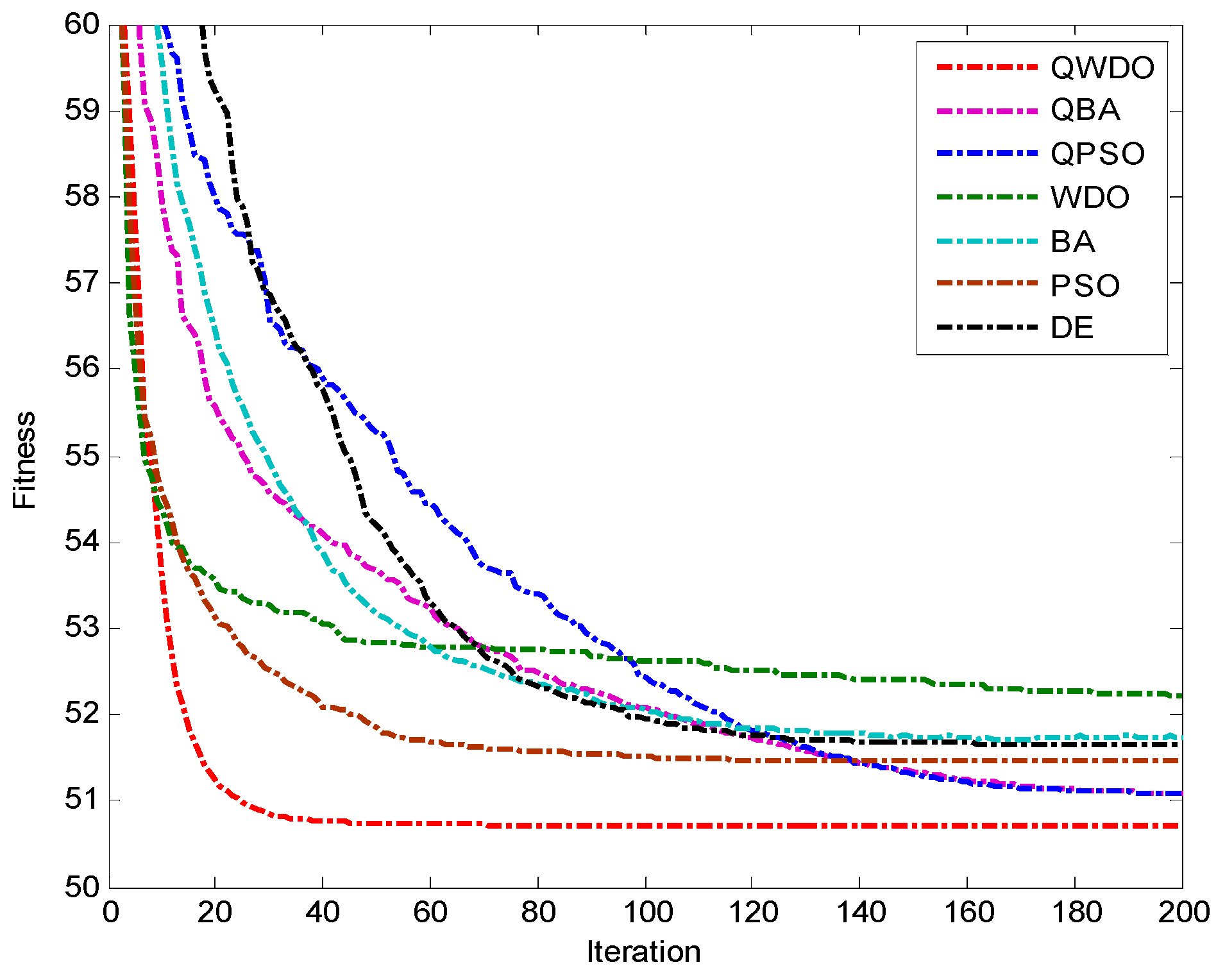
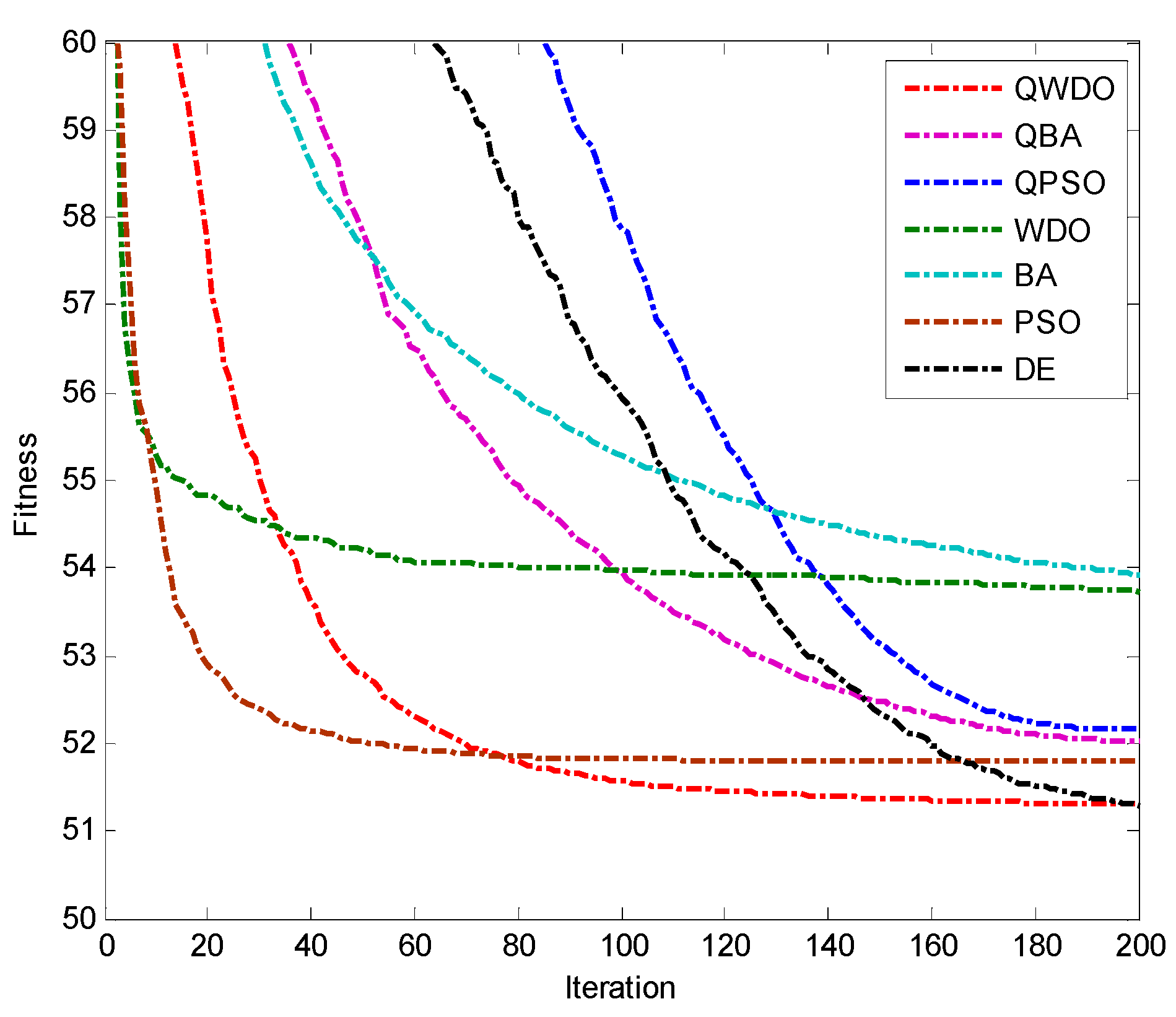
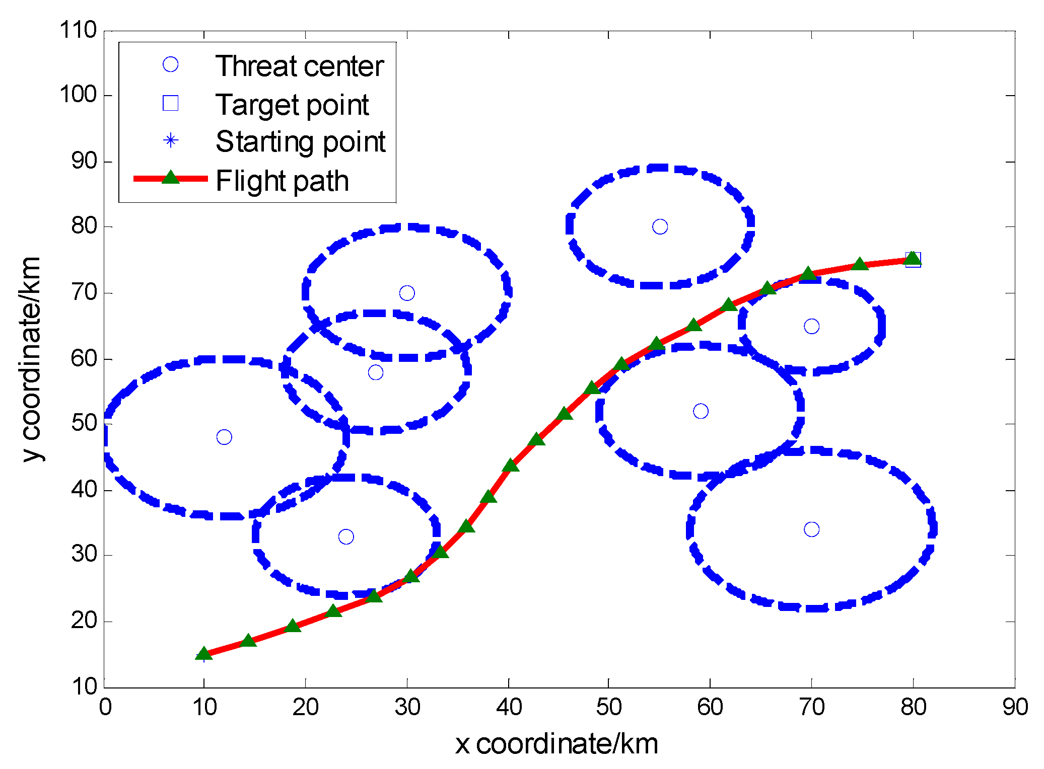
6.3. Experimental Results
| Threat Center (km) | (45,50) | (12,40) | (32,68) | (36,26) | (55,80) |
|---|---|---|---|---|---|
| Threat radius (km) | 10 | 10 | 8 | 12 | 9 |
| Threat grade | 2 | 10 | 1 | 2 | 3 |
| Popsize | Maxgen | D | Result | DE | PSO | BA | WDO | QPSO | QBA | QWDO |
|---|---|---|---|---|---|---|---|---|---|---|
| 30 | 200 | 5 | Mean | 59.47631887 | 69.69789792 | 79.69109684 | 71.34530853 | 63.43087561 | 68.98614459 | 68.96129066 |
| Best | 53.50706462 | 53.78972474 | 53.65716479 | 69.87539134 | 53.51528812 | 53.71340066 | 57.98320586 | |||
| Worst | 69.41083451 | 122.5251479 | 153.561503 | 74.74310818 | 69.65781726 | 69.70146844 | 69.34914343 | |||
| 30 | 200 | 10 | Mean | 51.65071551 | 51.46197291 | 51.63995084 | 52.22163684 | 51.09958359 | 51.09603877 | 50.7143172 |
| Best | 50.71342237 | 50.76572646 | 50.75929951 | 51.70051826 | 50.73093318 | 50.74767855 | 50.7133255 | |||
| Worst | 56.58333938 | 54.59093708 | 63.46628192 | 52.82754363 | 53.39086949 | 53.84706658 | 50.7210475 | |||
| 30 | 200 | 15 | Mean | 50.66037482 | 51.5051898 | 51.87380989 | 52.44224824 | 50.76853918 | 50.89080424 | 50.58231653 |
| Best | 50.44414089 | 50.71382405 | 50.50789696 | 51.60523312 | 50.48866711 | 50.49293993 | 50.44266169 | |||
| Worst | 53.13768683 | 55.0444921 | 60.46255447 | 53.11065178 | 53.31076469 | 53.69423022 | 54.54535767 | |||
| 30 | 200 | 20 | Mean | 50.72261529 | 51.45672198 | 53.35967758 | 52.97445056 | 51.07754398 | 51.0110708 | 50.99002665 |
| Best | 50.44379211 | 50.80930764 | 50.63331206 | 52.06541936 | 50.48490215 | 50.54761522 | 50.39488366 | |||
| Worst | 53.01708277 | 53.35679952 | 62.1522776 | 54.06882944 | 53.41618848 | 53.19280513 | 52.87373122 | |||
| 30 | 200 | 25 | Mean | 51.28794992 | 51.7891286 | 53.92302186 | 53.73746145 | 52.16273619 | 52.02298198 | 50.91502774 |
| Best | 50.48966734 | 50.99255379 | 50.80805259 | 51.49756894 | 50.92275235 | 50.67574917 | 50.38774681 | |||
| Worst | 57.87611595 | 54.01746732 | 58.78868887 | 54.84758084 | 54.91448413 | 54.12956224 | 55.70310267 |


| Popsize | Maxgen | D | Result | DE | PSO | BA | WDO | QPSO | QBA | QWDO |
|---|---|---|---|---|---|---|---|---|---|---|
| 30 | 50 | 20 | Mean | 51.55066072 | 57.49611763 | 55.52925757 | 53.37244656 | 55.06247744 | 53.26816353 | 51.0384824 |
| Best | 50.86230831 | 52.4021891 | 50.8335776 | 51.63208235 | 52.87505334 | 51.2628276 | 50.56417883 | |||
| Worst | 52.97970342 | 67.05488964 | 63.29522516 | 54.20131962 | 61.773734 | 58.6281585 | 53.31025066 | |||
| 30 | 100 | 20 | Mean | 51.51743739 | 52.44222368 | 53.18924498 | 53.40007277 | 52.13986363 | 51.53347574 | 51.04911419 |
| Best | 50.98301911 | 50.68878829 | 51.00545315 | 51.88063479 | 51.22499096 | 50.67123961 | 50.39932388 | |||
| Worst | 52.51570068 | 59.61227827 | 58.92518468 | 54.23101102 | 54.12993175 | 55.38455421 | 52.93418088 | |||
| 30 | 150 | 20 | Mean | 51.93773208 | 50.91881032 | 53.00666682 | 53.14375161 | 51.37913337 | 51.48087993 | 50.76428055 |
| Best | 50.76460097 | 50.41768377 | 50.6384468 | 51.90565475 | 50.63851986 | 50.61691071 | 50.39664491 | |||
| Worst | 59.1205155 | 53.27343125 | 61.22625354 | 54.01364469 | 55.1714668 | 54.98546674 | 52.91230338 | |||
| 30 | 200 | 20 | Mean | 50.73461503 | 51.67395413 | 53.26005394 | 53.15550115 | 51.39219052 | 51.02583378 | 50.58751325 |
| Best | 50.4160651 | 50.91067104 | 50.62680554 | 52.15259159 | 50.51985597 | 50.5578439 | 50.39570371 | |||
| Worst | 53.33085477 | 54.17616743 | 61.10842324 | 54.17028213 | 53.93215589 | 53.50379863 | 52.86341706 | |||
| 30 | 250 | 20 | Mean | 51.46928513 | 50.7031705 | 52.63088516 | 52.89985245 | 50.88980761 | 51.34376512 | 50.91479454 |
| Best | 50.78648292 | 50.42161575 | 50.5392192 | 51.96380792 | 50.49328732 | 50.49715669 | 50.39447178 | |||
| Worst | 54.08790265 | 53.06705989 | 60.68415725 | 53.67059243 | 53.42973728 | 57.02850459 | 52.8744808 |
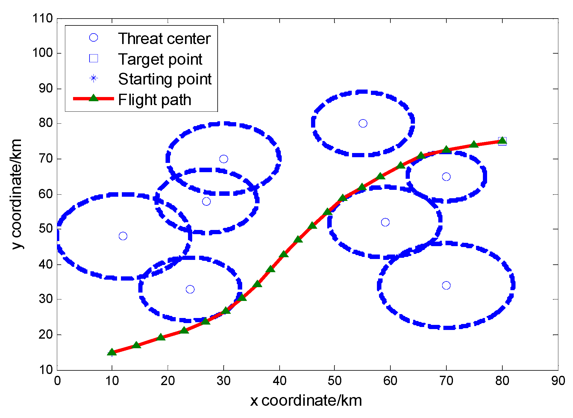
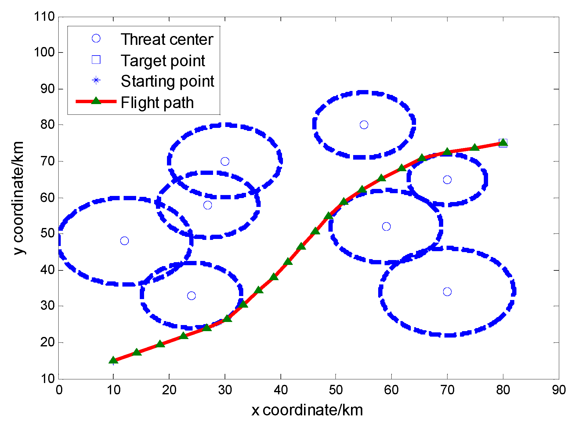
| Threat Center | (59,52) | (55,80) | (27,58) | (24,33) | (12,48) | (70,65) | (70,34) | (30,70) |
|---|---|---|---|---|---|---|---|---|
| Threat radius | 10 | 9 | 9 | 9 | 12 | 7 | 12 | 10 |
| Threat level | 9 | 7 | 3 | 12 | 1 | 5 | 13 | 2 |
| Popsize | Maxgen | D | Result | DE | PSO | BA | WDO | QPSO | QBA | QWDO |
|---|---|---|---|---|---|---|---|---|---|---|
| 30 | 200 | 5 | Mean | 108.4500391 | 76.32274731 | 217.8576809 | 158.6365421 | 58.55026343 | 224.8713213 | 86.06651884 |
| Best | 51.51154424 | 51.51285958 | 51.62725599 | 53.3969487 | 51.52283974 | 51.56102341 | 51.51142514 | |||
| Worst | 257.7693771 | 259.3727002 | 262.6262155 | 779.1292284 | 258.96214051 | 263.0166854 | 257.7692998 | |||
| 30 | 200 | 10 | Mean | 51.69531753 | 59.62698855 | 56.56107653 | 66.95686144 | 51.28710941 | 56.49182092 | 52.58309128 |
| Best | 48.21839521 | 48.60012275 | 48.31096493 | 51.14078655 | 48.2522368 | 48.30357221 | 48.21752061 | |||
| Worst | 60.65282489 | 71.23964789 | 63.92306031 | 102.9043651 | 61.60174489 | 66.80983521 | 60.56959953 | |||
| 30 | 200 | 15 | Mean | 50.073766 | 53.86901522 | 50.86134423 | 66.95568288 | 49.52489924 | 50.95870139 | 49.50373784 |
| Best | 47.93535622 | 50.43482837 | 48.06959155 | 57.01360885 | 48.01888001 | 48.13432924 | 47.86853465 | |||
| Worst | 51.57555205 | 59.96256435 | 52.76505672 | 74.82060029 | 51.6348462 | 56.00698594 | 50.82801702 | |||
| 30 | 200 | 20 | Mean | 49.84233544 | 51.48149235 | 50.90193378 | 66.66824246 | 49.67928022 | 50.07122862 | 48.81483482 |
| Best | 48.12672661 | 49.24653359 | 48.16350755 | 58.430756 | 48.39737111 | 48.33316163 | 47.80715661 | |||
| Worst | 52.11021304 | 54.24689277 | 67.44172011 | 75.96794054 | 51.30798995 | 53.42378109 | 49.74939729 | |||
| 30 | 200 | 25 | Mean | 50.66805474 | 50.95517305 | 51.34776811 | 71.70637996 | 50.83847029 | 50.60934221 | 48.59295541 |
| Best | 48.70720514 | 49.54338148 | 48.79658763 | 59.14948465 | 48.75545861 | 48.39299019 | 47.83424938 | |||
| Worst | 55.79533973 | 53.49953637 | 64.50598736 | 80.26246808 | 53.58558572 | 53.91518696 | 49.45543938 |
| Popsize | Maxgen | D | Result | DE | PSO | BA | WDO | QPSO | QBA | QWDO |
|---|---|---|---|---|---|---|---|---|---|---|
| 30 | 50 | 20 | Mean | 60.11210553 | 52.10944247 | 54.69506882 | 75.33956531 | 54.98617763 | 53.48694368 | 50.04535423 |
| Best | 54.63302708 | 49.63615429 | 49.15087344 | 64.96697732 | 51.63957205 | 49.77944089 | 48.06638554 | |||
| Worst | 68.85463056 | 55.49586702 | 68.94866149 | 96.58202587 | 61.59178853 | 57.49410513 | 54.18169722 | |||
| 30 | 100 | 20 | Mean | 53.83836816 | 51.36653616 | 53.14143773 | 70.57187552 | 51.38397481 | 50.46414355 | 49.02122905 |
| Best | 48.33976811 | 49.07513681 | 48.69510082 | 57.67068514 | 48.99505905 | 48.42088512 | 47.86003025 | |||
| Worst | 60.13601866 | 53.46121189 | 75.25004292 | 83.08842351 | 55.59578695 | 54.24391665 | 50.15146747 | |||
| 30 | 150 | 20 | Mean | 51.05336892 | 51.57677078 | 50.84575891 | 70.54479972 | 50.45391734 | 50.39693696 | 48.72957492 |
| Best | 49.40096571 | 49.67670378 | 48.62648502 | 62.80958025 | 48.41389406 | 48.52347097 | 47.82128972 | |||
| Worst | 55.88497818 | 54.28141398 | 61.23851396 | 76.00858334 | 52.69768873 | 53.3014373 | 49.54581499 | |||
| 30 | 200 | 20 | Mean | 49.9035051 | 51.5013683 | 50.16504165 | 69.76739786 | 49.73289806 | 49.82207652 | 48.67284272 |
| Best | 48.39387138 | 49.74179751 | 48.44930632 | 62.87834457 | 48.17837129 | 48.31338872 | 47.80987825 | |||
| Worst | 50.94635705 | 54.31102253 | 61.2292916 | 76.48909998 | 51.56006612 | 52.70993366 | 49.85033671 | |||
| 30 | 250 | 20 | Mean | 49.6679397 | 51.96561739 | 50.3002217 | 67.90792328 | 49.25710679 | 49.76274007 | 48.78279719 |
| Best | 47.94541607 | 50.42009286 | 48.23889332 | 60.92844125 | 48.12683235 | 48.16417909 | 47.80721825 | |||
| Worst | 52.17249675 | 55.53271834 | 61.53309025 | 77.23621705 | 50.74799695 | 52.16236524 | 49.51742143 |


7. Conclusion and Future Research
Acknowledgments
Author Contributions
Conflicts of Interest
References
- Ma, Q.; Lei, X. Application of improved particle swarm optimization algorithm in UCAV path planning. Artif. Intell. Computat. Intell. 2009, 5855, 206–214. [Google Scholar]
- Ma, Q.; Lei, X. Application of artificial fish school algorithm in UCAV path planning. In Proceeding of the 2010 IEEE Fifth International Conference on Bio-Inspired Computing: Theories and Applications (BIC-TA), Changsha, China, 23–26 September 2010; pp. 555–559.
- Duan, H.B.; Zhang, X.Y.; Xu, C.F. Bio-Inspired Computing; Science Press: Beijing, China, 2011. [Google Scholar]
- Wang, G.; Guo, L.; Duan, H.; Liu, L.; Wang, H. A bat algorithm with mutation for UCAV path planning. Sci. World J. 2012, 2012. [Google Scholar] [CrossRef]
- Wang, G.; Guo, L.; Duan, H.; Liu, L.; Wang, H. A modified firefly algorithm for UCAV path planning. Int. J. Hybrid Inf. Technol. 2012, 5, 123–144. [Google Scholar]
- Li, B.; Gong, L.; Yang, W. An improved artificial bee colony algorithm based on balance-evolution strategy for unmanned combat aerial vehicle path planning. Sci. World J. 2014, 2014. [Google Scholar] [CrossRef] [PubMed]
- Zhou, Q.; Zhou, Y.; Chen, X. A Wolf Colony Search Algorithm Based on the Complex Method for Unmanned Combat Air Vehicle Path Planning. Int. J. Hybrid Inf. Technol. 2014, 7, 183–200. [Google Scholar] [CrossRef]
- Zhu, W.; Duan, H. Chaotic predator-prey biogeography-based optimization approach for UCAV path planning. Aerosp. Sci. Technol. 2014, 32, 153–161. [Google Scholar] [CrossRef]
- Bayraktar, Z.; Komurcu, M.; Werner, D.H. Wind Driven Optimization (WDO): A novel nature-inspired optimization algorithm and its application to electromagnetics. In Proceeding of the Antennas and Propagation Society International Symposium (APSURSI), Toronto, ON, Canada, 11–17 July 2010; pp. 1–4.
- Bayraktar, Z.; Komurcu, M.; Bossard, J.A.; Werner, D. The wind driven optimization technique and its application in electromagnetics. IEEE Trans. Antennas Propag. 2013, 61, 2745–2757. [Google Scholar] [CrossRef]
- Bhandari, A.K.; Singh, V.K.; Kumar, A.; Singh, G. Cuckoo search algorithm and wind driven optimization based study of satellite image segmentation for multilevel thresholding using Kapur’s entropy. Expert Syst. Appl. 2014, 41, 3538–3560. [Google Scholar] [CrossRef]
- Sun, J.; Wang, X.; Huang, M.; Gao, C. A Cloud Resource Allocation Scheme Based on Microeconomics and Wind Driven Optimization. In Proceeding of the 2013 8th Conference on ChinaGrid Annual Conference (ChinaGrid), Changchun, China, 22–23 August 2013; pp. 34–39.
- Boulesnane, A.; Meshoul, S. A new multi-region modified wind driven optimization algorithm with collision avoidance for dynamic environments. Adv. Swarm Intell. Springer Int. Publ. 2014, 8795, 412–421. [Google Scholar]
- Kuldeep, B.; Singh, V.K.; Kumar, A.; Singh, G.K. Design of two-channel filter bank using nature inspired optimization based fractional derivative constraints. ISA Trans. 2015, 54, 101–116. [Google Scholar] [CrossRef] [PubMed]
- Mahto, S.K.; Choubey, A.; Suman, S. Linear array synthesis with minimum side lobe level and null control using wind driven optimization. In proceeding of the 2015 International Conference on Signal Processing And Communication Engineering Systems (SPACES), Guntur, India, 2–3 January 2015; pp. 191–195.
- Yang, X.S. Nature-Inspired Optimization Algorithms; Elsevier: San Francisco, CA, USA, 2014. [Google Scholar]
- Li, S.Y.; Li, P.C. Quantum particle swarms algorithm for continuous space optimization. Chin. J. Quantum Electron. 2007, 24, 569–574. (In Chinese) [Google Scholar]
- Duan, H.; Li, P. Bio-Inspired Computation in Unmanned Aerial Vehicles; Springer Berlin Heidelberg: Berlin, Germany, 2014. [Google Scholar]
- Xu, C.; Duan, H.; Liu, F. Chaotic artificial bee colony approach to Unmanned Combat Air Vehicle (UCAV) path planning. Aerosp. Sci. Technol. 2010, 14, 535–541. [Google Scholar] [CrossRef]
- Li, P.; Duan, H.B. Path planning of unmanned aerial vehicle based on improved gravitational search algorithm. Sci. China Technol. Sci. 2012, 55, 2712–2719. [Google Scholar] [CrossRef]
- Riehl, H. Introduction to the Atmosphere; McGraw Hill: New York, NY, USA, 1978. [Google Scholar]
- Ahrens, C.D. Meteorology Today: An Introduction to Weather, Climate, and the Environment, 7th ed.; Thomson-Brook/Cole: Belmont, CA, USA, 2003. [Google Scholar]
- Hey, T. Quantum computing: An introduction. Comput. Control Eng. J. 1999, 10, 105–112. [Google Scholar] [CrossRef]
- Li, Z.Y.; Ma, L.; Zhang, H.Z. Quantum bat algorithm for function optimization. J. Syst. Manag. 2014, 21, 717–722. (In Chinese) [Google Scholar]
- Soares, J.; Silva, M.; Vale, Z.; de Moura Oliveira, P.B. Quantum-based PSO applied to hour-ahead scheduling in the context of smart grid management. In proceeding of the 2015 IEEE Eindhoven on PowerTech, Eindhoven, Dutch, 29 June–2 July 2015; pp. 1–6.
© 2015 by the authors; licensee MDPI, Basel, Switzerland. This article is an open access article distributed under the terms and conditions of the Creative Commons Attribution license (http://creativecommons.org/licenses/by/4.0/).
Share and Cite
Zhou, Y.; Bao, Z.; Wang, R.; Qiao, S.; Zhou, Y. Quantum Wind Driven Optimization for Unmanned Combat Air Vehicle Path Planning. Appl. Sci. 2015, 5, 1457-1483. https://doi.org/10.3390/app5041457
Zhou Y, Bao Z, Wang R, Qiao S, Zhou Y. Quantum Wind Driven Optimization for Unmanned Combat Air Vehicle Path Planning. Applied Sciences. 2015; 5(4):1457-1483. https://doi.org/10.3390/app5041457
Chicago/Turabian StyleZhou, Yongquan, Zongfan Bao, Rui Wang, Shilei Qiao, and Yuxiang Zhou. 2015. "Quantum Wind Driven Optimization for Unmanned Combat Air Vehicle Path Planning" Applied Sciences 5, no. 4: 1457-1483. https://doi.org/10.3390/app5041457
APA StyleZhou, Y., Bao, Z., Wang, R., Qiao, S., & Zhou, Y. (2015). Quantum Wind Driven Optimization for Unmanned Combat Air Vehicle Path Planning. Applied Sciences, 5(4), 1457-1483. https://doi.org/10.3390/app5041457