Article

Cross-Regional Hyperspectral Estimation of Soil Organic Carbon in Eurasian Black Soils Using an Optimal Spectral Feature Set


1
College of Geo-Exploration Science and Technology, Jilin University, Changchun 130026, China
2
School of Modern Industry, Jilin Jianzhu University, Changchun 130118, China
*
Author to whom correspondence should be addressed.
Appl. Sci. 2026, 16(9), 4433; https://doi.org/10.3390/app16094433
Submission received: 17 March 2026 / Revised: 24 April 2026 / Accepted: 29 April 2026 / Published: 1 May 2026

Abstract

Soil organic carbon (SOC) plays a critical role in the global carbon cycle and agroecosystem productivity. However, existing hyperspectral inversion models often exhibit significant predictive biases when applied across large geographic scales, primarily due to the spatial heterogeneity of pedogenic environments and background mineralogy. This study proposes a cross-regional SOC prediction method based on an optimal spectral feature set (SOC-OSFS). Leveraging laboratory hyperspectral and SOC data from 17,730 samples collected across the black soil regions of Northeast China and Europe, a core spectral feature set comprising 31 diagnostic bands was extracted using the competitive adaptive reweighted sampling (CARS) algorithm combined with the successive projections algorithm (SPA). Although this SOC-OSFS accounts for merely 1.55% of the original full-spectrum dimensionality (31 out of 2000 bands), it demonstrated robust analytical capability in local modeling across all study regions, yielding coefficients of determination (R2 = 0.6714–0.8854). When transferring the prediction model calibrated in the core source domain (n = 10,000) to the other seven independent typical black soil target domains, the direct cross-regional prediction consistently reduced the root mean square error (RMSE) by over 15% compared to that of the full-spectrum models. By further incorporating 20% of the local background samples for intercept correction, the cross-regional predictive accuracy was substantially improved; the goodness-of-fit for the Northeast China target domains increased sharply (maximum R2 = 0.8567), and the European target domains, which feature substantially different pedogenic environments, were successfully corrected from negative to positive linear fits. This study validates the efficacy of extracting physiochemically meaningful spectral bands in mitigating the interference caused by spatial heterogeneity, thereby providing a mechanistically grounded and practically viable framework for large-scale SOC estimation via remote sensing.

1. Introduction

As an invaluable global agricultural soil resource, black soil not only serves as a crucial foundation for ensuring food security but also acts as a vital carbon sequestration pool in terrestrial ecosystems [1,2,3,4]. However, influenced by climate change and long-term agricultural cultivation, the surface soil organic carbon (SOC) in black soil regions is facing a severe risk of depletion [3,5,6,7]. Fluctuations in its carbon sink capacity are intricately linked to the sustainability of regional agriculture and feedback to the climate system [8,9]. Therefore, exploring SOC estimation methods that transcend geographical boundaries holds significant practical implications for the conservation and dynamic monitoring of black soil resources [10,11].
In recent years, hyperspectral remote sensing has made substantial progress in SOC inversion [12,13,14]. However, existing estimation models often exhibit inherent spatial limitations when applied to study areas with large geographical spans [15,16,17,18]. This degradation in predictive performance primarily stems from the spatial heterogeneity of soil spectral responses: the interactive effects of varying pedogenic parent materials, soil textures, and background mineralogy across different geographical units lead to significant shifts of soil samples within the spectral feature space [19,20]. Because current modeling paradigms heavily rely on locally representative samples, they are prone to predictive biases when encountering heterogeneous pedogenic environments, which to some extent constrains the cross-regional synergistic utilization of soil spectral library resources [17,21,22].
Regarding hyperspectral estimation methods, early studies mostly attempted to simplify the quantitative estimation of SOC by constructing empirical spectral indices [23,24]. Although these methods possess a certain degree of physical interpretability, their simplistic structures make it difficult to comprehensively capture the latent physicochemical characteristics within high-dimensional spectral data [24,25,26]. With the evolution of data processing technologies, the research focus has gradually shifted towards spectral feature selection [27,28,29]. However, within a high-dimensional spectral space containing thousands of bands, a massive number of redundant variables not only capture the characteristic responses of organic matter but are also heavily confounded by environmental background noise dominated by soil moisture, iron oxides, and clay minerals [30,31,32,33]. How to effectively decouple these varying background interferences and extract feature bands supported by explicit physicochemical mechanisms—thereby mitigating the spatial heterogeneity issues caused by pedogenic differences—remains a crucial research direction that requires in-depth exploration in current hyperspectral soil property inversion [31,32,34].
Recently, various state-of-the-art techniques, including advanced deep learning architectures and complex transfer learning frameworks, have been increasingly applied to enhance hyperspectral SOC predictions [22,35,36,37,38]. While these sophisticated data-driven models have achieved high predictive accuracy at local or regional scales, with reported R2 values often exceeding 0.80 under controlled conditions [39,40,41], they often lack explicit incorporation of physicochemical mechanisms underlying soil spectral responses [37,42]. Furthermore, when directly extrapolated to macro-scales (e.g., transcontinental levels), these highly complex models frequently suffer from severe performance degradation due to unmitigated systematic biases caused by varying pedogenic environments [43,44,45]. In contrast to these computationally intensive and data-demanding paradigms, which primarily rely on statistical learning from high-dimensional spectral space, our study advocates for a more transparent and mechanism-driven approach. By explicitly decoupling background noise through an optimized feature selection strategy prior to modeling, and coupling it with a highly efficient local sample fine-tuning (spiking) technique, our framework provides a robust and practically feasible solution for mitigating transcontinental prediction biases.
To address the limited spatial applicability of existing models [22], this study takes the black soil regions of Northeast China and Europe as research targets, aiming to explore the spectral response patterns of SOC across geographical boundaries and provide a feature extraction-based framework for cross-regional inversion. Rather than developing new fundamental algorithms, the primary contribution of this study lies in the integrated application of established methods to mitigate systematic biases in cross-regional SOC prediction. First, this study introduces the competitive adaptive reweighted sampling (CARS) and successive projections algorithm (SPA) to strip away environmental background noise from the full-spectrum data [46], extracting an optimal spectral feature set for SOC that is supported by the physicochemical mechanisms of macromolecular functional groups [47,48,49]. Second, by comparing the spectral distributions of the full-spectrum data and the optimal feature set via principal component analysis (PCA) [18,50,51], we verify the role of feature band extraction in suppressing background mineral interference and achieving cross-regional feature space realignment. Finally, multi-algorithm comparative experiments are designed to evaluate the performance of the cross-regional prediction method, which is based on the optimal spectral feature set combined with a small number of local target samples for intercept correction (spiking) [16,34,52,53]. This study aims to provide a novel and practical framework for mitigating the impact of pedogenic environmental differences on hyperspectral inversion models, by integrating physically interpretable spectral features with cross-regional transfer strategies for large-scale SOC estimation.

2. Materials

2.1. Study Areas

To investigate the stability of spectral characteristics of soil organic carbon (SOC) across different geographical spatial scales, this study focused on typical black soil regions to construct a hierarchical soil spectral dataset encompassing three progressive scales: “local–regional–intercontinental.”
The Hailun (HL) region, located in the Northeast China black soil belt, was selected as the core study area. Situated in the core zone of cold-region black soils in the Songnen Plain, the primary soil type in this region is typical thin-layer Chernozem [54]. The HL dataset comprises 10,000 topsoil samples, featuring an extensive sample size and a comprehensive SOC concentration gradient, thus serving as the primary source domain for spectral feature extraction.
Seven other typical black soil domains were selected as cross-regional target (validation) sets, including four in Northeast China and three in Europe. The target regions in Northeast China encompass Baoqing (BQ), Qiqihar (QQH), Fuyuan-Fujin (FYFJ), and Jilin (JL), with soil types covering typical black soils, sandy black soils, and meadow black soils (Phaeozems). The European black soil target regions comprise Austria (AT), the Czech Republic (CZ), and Hungary (HU), predominantly characterized by Chernozems [54].

2.2. Data

A total of 17,526 samples from the Northeast China black soil belt were collected during field campaigns in 2017, including HL (n = 10,000), BQ (n = 6361), QQH (n = 651), FYFJ (n = 397), and JL (n = 117). Specifically, the raw dataset in the HL region was subjected to strict quality control to remove samples with anomalous spectral responses and SOC measurement errors, resulting in a final dataset of 10,000 valid samples for subsequent analysis. The SOC contents of these soil samples were analyzed using the laboratory potassium dichromate volumetric method (DZ/T 0279), which shares the same analytical principle as the Walkley-Black method [55,56]. To ensure the consistency of spectral quality [31,32,57], soil sample preparation (air-drying, grinding, and sieving) and spectral measurements strictly followed standardized laboratory protocols under consistent environmental conditions, effectively minimizing the influence of soil moisture variability and surface heterogeneity on spectral measurements [2,45,58]. Spectral measurements were acquired using two distinct spectrometers: the ASD FieldSpec® 3 (FS3) and the ASD FieldSpec® 4 (FS4) (Analytical Spectral Devices, Inc., Boulder, CO, USA). To eliminate systematic instrumental biases, the Internal Soil Standard (ISS) method was applied to align the FS4 data to the FS3 standard [31,32,58,59], thereby minimizing potential systematic discrepancies between instruments and ensuring cross-sensor comparability.
The 204 European black soil samples utilized in this study were extracted from the LUCAS 2009 topsoil database [60], comprising AT (n = 40), CZ (n = 29), and HU (n = 135). The spectral data of these samples were resampled to a 1-nm interval to align spectrally with the Chinese dataset.
The spatial distribution of the aforementioned 17,730 black soil sampling sites is illustrated in Figure 1. For all spectral data, the marginal noisy bands (350–400 nm and 2401–2500 nm) were truncated, retaining the core wavelength range of 401–2400 nm. Subsequently, the Savitzky–Golay (SG) smoothing filter was applied across the full spectral dimensions to enhance the signal-to-noise ratio [61].

3. Methods

3.1. Spectral Transformation Methods

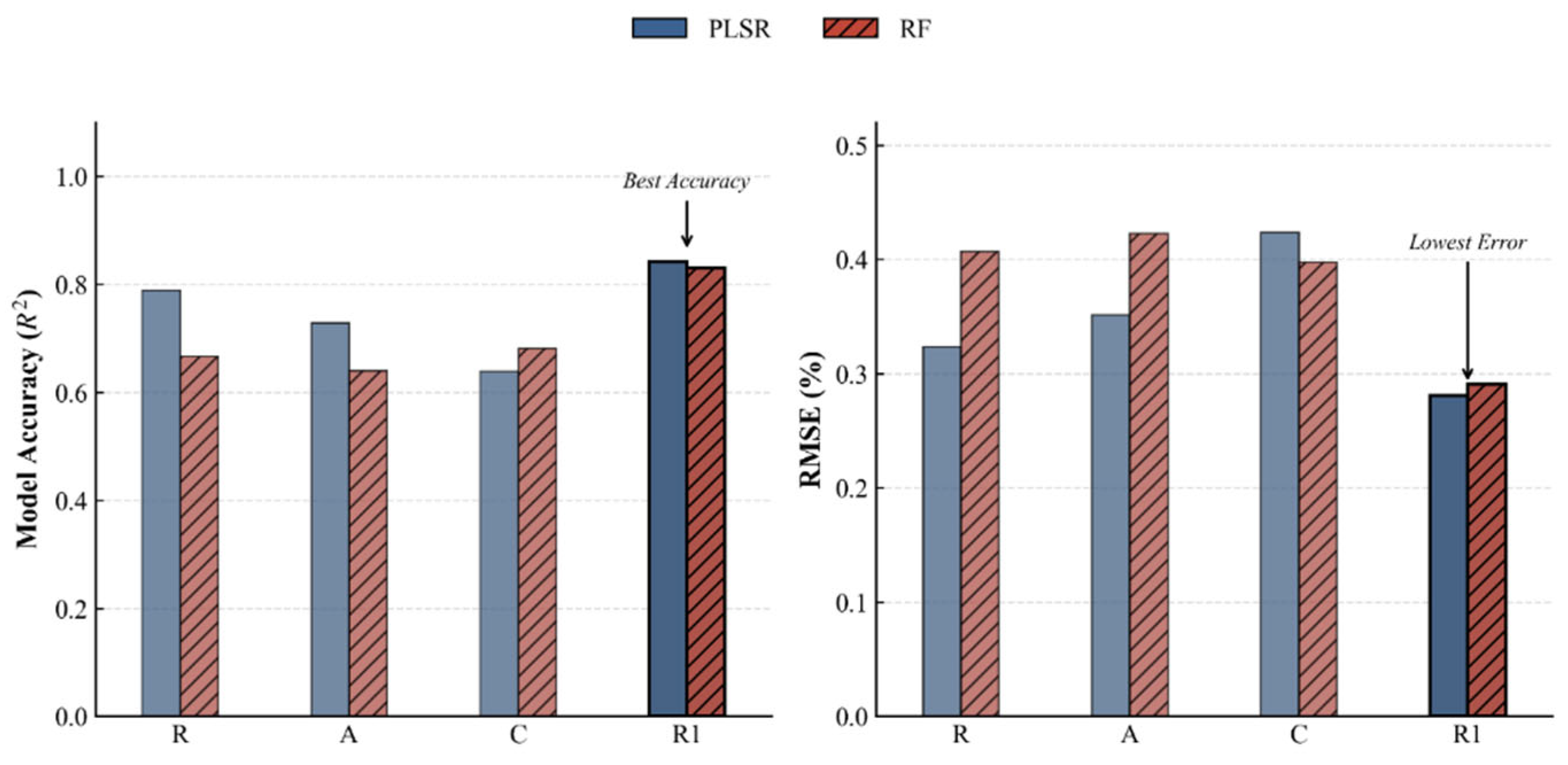
To enhance data robustness and isolate the optimal spectral responses of SOC, this study compared four spectral transformation forms: raw reflectance (R), first derivative (R′), continuum removal (C), and absorbance (A) [48]. Preliminary experimental results based on the core study area (HL) (Figure 2) demonstrated that the Partial Least Squares Regression (PLSR) and Random Forest (RF) models achieved the highest accuracy and the lowest error after applying the first derivative transformation. Consistent with previous findings [62], the first derivative (R′) effectively mitigates the baseline drift inherent in black soil backgrounds and amplifies the characteristic absorption peaks of SOC, thereby improving the sensitivity of the spectra to SOC content. Consequently, the first derivative (R′) was selected as the foundational spectral form for subsequent feature extraction and model construction. The calculation is expressed as Equation (1):
R λ i = R λ i + 1 R λ i 1 2 Δ λ
where λ i represents the wavelength of the i -th band; R λ i is the first derivative value at wavelength λ i ; R λ i + 1 and R λ i 1 are the original reflectance values at the wavelengths immediately adjacent to λ i ; and Δ λ is the wavelength interval between adjacent bands.

3.2. Feature Space and Feature Band Extraction

3.2.1. Feature Space Construction and Visualization

To quantitatively assess the similarities and disparities in SOC spectral responses across different regions, Principal Component Analysis (PCA) was applied to the first derivative (R′) spectra. The first two principal components (PC1 and PC2) were extracted, as they accounted for the largest proportion of variance. These components were then used to construct a two-dimensional feature space. To intuitively visualize the heterogeneity of the cross-regional data distribution, samples from the core study area (HL) were used as the baseline. Samples from other regions were then overlaid as colored scatter points. By comparing the degree of overlap and the direction of shift of samples from various regions within the PC1-PC2 coordinate system, the impact of regional soil variations on spectral responses was qualitatively evaluated.

3.2.2. Feature Band Extraction Method

High-dimensional hyperspectral data often suffer from redundancy and multicollinearity. To address this issue, a two-stage hybrid feature extraction framework was developed, combining Competitive Adaptive Reweighted Sampling (CARS) and the Successive Projections Algorithm (SPA). This approach aims to filter out interference signals driven by environmental backgrounds (e.g., dynamic moisture changes and non-specific minerals) and extract universally applicable feature bands. Initially, CARS was employed for global coarse screening, utilizing an exponentially decreasing function to rapidly eliminate uninformative variables. Subsequently, SPA was introduced for local refinement, employing orthogonal projections in a vector space to maximally eradicate collinear redundancy among the bands. Finally, the selected subset of feature bands was mapped onto the mean spectral curve of the soil samples to mechanistically validate whether they precisely correspond to the characteristic absorption bands of SOC-related core functional groups.

3.3. SOC Estimation Models and Accuracy Evaluation Metrics

3.3.1. SOC Estimation Model Construction

To verify the robustness of the extracted feature bands, a gradient model matrix encompassing linear and nonlinear, as well as shallow and deep architectures, was constructed. Specifically, Partial Least Squares Regression (PLSR), a classical model for soil spectral modeling, was selected as the linear baseline model [63,64], while Random Forest (RF), a traditional machine learning algorithm, served as the nonlinear baseline model [65]. To further unearth the application potential of the feature bands, two prominent deep learning architectures were incorporated: Convolutional Neural Networks (CNN) and Long Short-Term Memory networks (LSTM). The CNN focused on extracting local spatial-spectral features [66], whereas the LSTM emphasized analyzing long-range dependencies within the spectral sequences [67].

3.3.2. Model Evaluation Metrics

To accurately quantify the evolution of model predictive performance, an accuracy evaluation system was established using four metrics: Coefficient of Determination ( R 2 ), Root Mean Square Error (RMSE), Ratio of Performance to Deviation (RPD), and Bias. To eliminate the randomness associated with sample partitioning, all models were subjected to 50 Monte Carlo simulations to verify their spatial predictive stability. The calculation formulas for these metrics are as follows:
R 2 = 1 i = 1 n y i ^ y i 2 i = 1 n y i y ¯ 2
R M S E = 1 n i = 1 n y i ^ y i 2
R P D = S D R M S E
B i a s = 1 n i = 1 n y i ^ y i
where n represents the total number of samples; y i and y i ^ denote the measured and predicted values, respectively; y ¯ is the mean of the measured values; and S D is the standard deviation of the measured values.

4. Results

4.1. SOC Data Distribution and Spatial Heterogeneity Analysis

Prior to feature extraction and cross-regional model construction, a statistical analysis of the SOC content in the core study area (HL) and the other seven validation regions was conducted, with the results presented in Table 1. As the core study area, the HL dataset exhibits robust statistical representativeness, comprising 10,000 samples with a broad SOC concentration gradient ranging from 0.17% to 8.80%, a mean of 2.51%, and a coefficient of variation (CV) of 28.09%. This distribution—characterized by a wide gradient, massive sample size, and moderate variability—provides robust data support for the subsequent research.
In contrast, the validation regions exhibit pronounced spatial heterogeneity. Within the Northeast China black soil belt, Baoqing (BQ), serving as the largest validation region (n = 6361), reached a maximum SOC value of 20.30%, significantly expanding the upper concentration limit of SOC in this region; the JL region demonstrated an exceptionally high CV of 65.21%, reflecting extreme local spatial dispersion; furthermore, the mean SOC in Qiqihar (QQH) was 3.18%, markedly higher than that in the HL region, reflecting an overall elevated distribution pattern. Among the European validation regions (AT, CZ, HU), SOC contents were generally lower. The mean values were clustered between 1.84% and 1.96%. In addition, the distribution patterns differed substantially from those observed in the Chinese regions. While the Chinese black soil regions generally exhibited a long-tailed positive skewness, the Hungarian (HU) dataset displayed a skewness of −0.07, indicating a slight negative skew. These macroscopic statistical discrepancies objectively reflect the significant heterogeneity in pedogenic environments and background properties across Eurasian black soils.
Collectively, these distributional results demonstrate that black soil SOC across different geographical spaces exhibits strong background disparities and spatial variations, which constitute the primary source of error when directly utilizing full-spectrum data for cross-regional remote sensing inversion.

4.2. Feature Band Extraction Results

4.2.1. Two-Stage Hybrid Feature Extraction Based on CARS-SPA

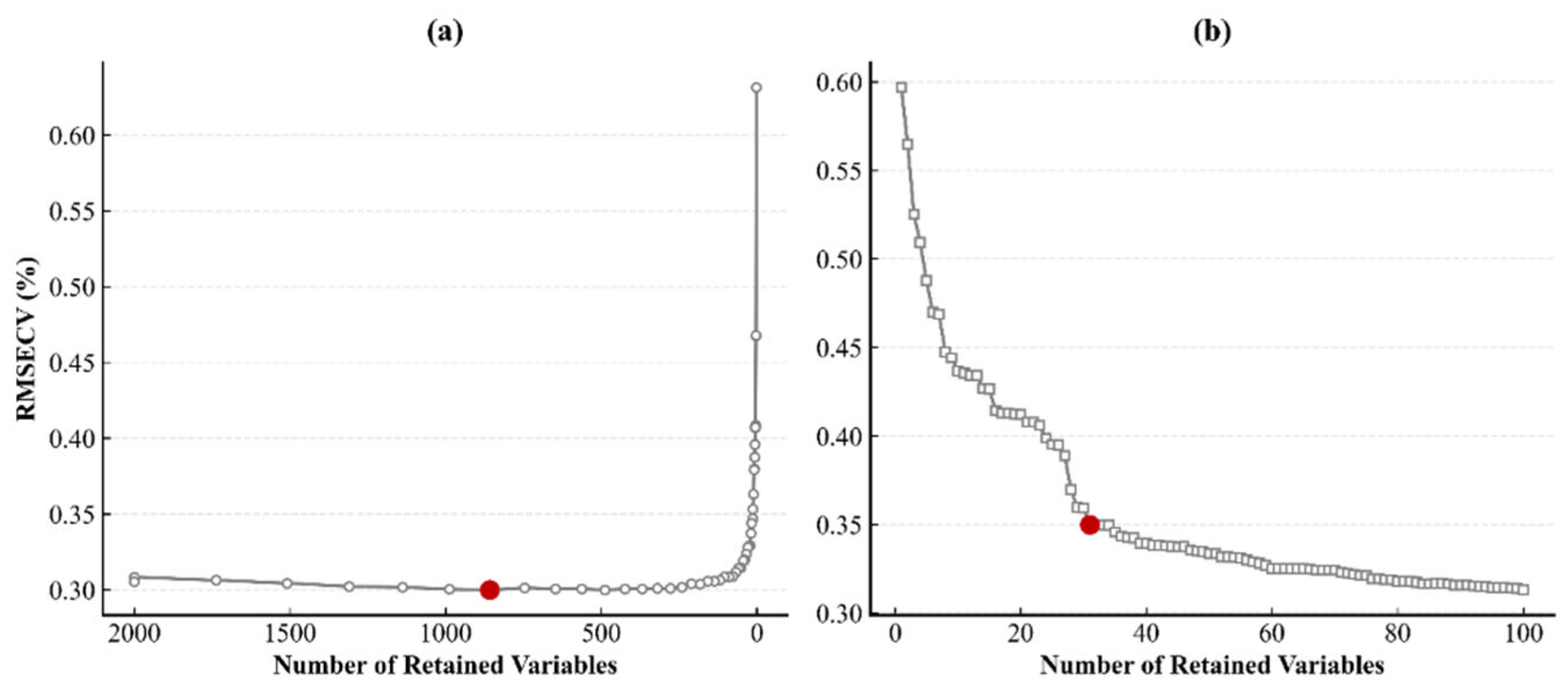
The full-spectrum data of the core study area (HL) comprised 2000 variables. This study applied a two-stage hybrid feature extraction method combining CARS and SPA, whose error evolution and iterative optimization process are illustrated in Figure 3. Initially, CARS was applied for global coarse screening. During this phase, the RMSECV first decreased and then increased sharply. This pattern reflects the progressive elimination of uninformative variables. After 50 iterations, the error reached a global minimum of 0.2999 when 858 variables were retained. Although this stage discarded over 50% of the bands, the retained subset still harbored high dimensional redundancy.
Subsequently, SPA was employed for secondary dimensionality reduction. As shown in Figure 3b, the error curve dropped sharply at first before gradually plateauing as the number of feature variables increased. Based on geometric distance calculations, an optimal “elbow point” emerged at a variable dimension of N = 31 (RMSECV = 0.3499). Beyond this threshold, the accuracy gains from introducing new bands tended to saturate. Considering both model fitting accuracy and cross-regional generalization capability, and to effectively prevent feature overfitting to the HL samples, these 31 critical bands were ultimately finalized as the SOC Optimal Spectral Feature Set (SOC-OSFS). Accounting for merely 1.55% of the original full-spectrum dimensionality, the SOC-OSFS efficiently purified the target core spectral information while stripping away the vast majority of background noise.

4.2.2. Validation of SOC-OSFS Spectral Responses

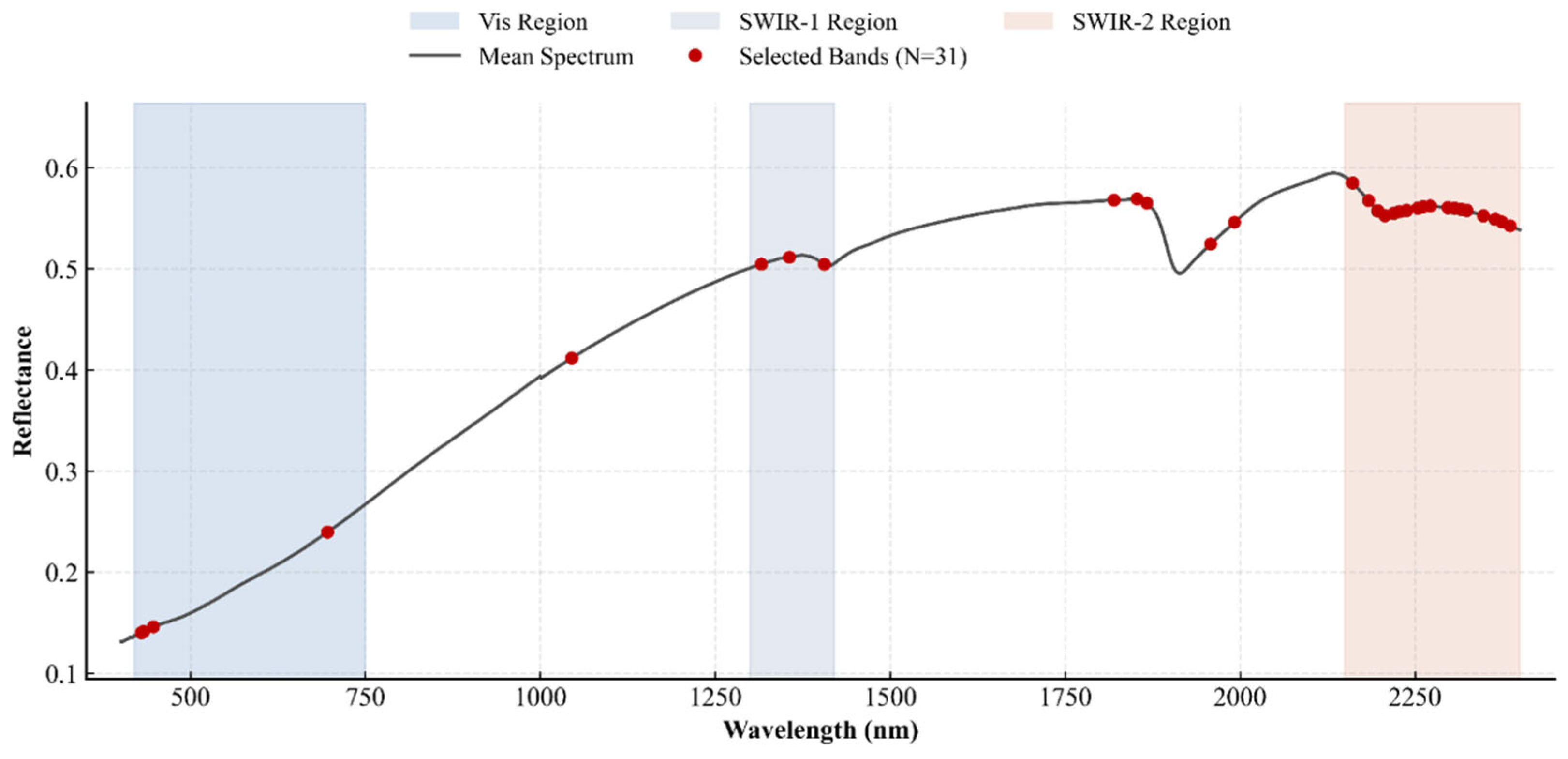
Mapping the 31 feature bands of the SOC-OSFS onto the mean spectral curve of the samples revealed a clear association between their spatial distribution and known soil organic matter absorption regions, as detailed in Figure 4. Within the visible region (Vis, 401–700 nm), the SOC-OSFS captured three bands: 430, 433, and 447 nm. These bands are commonly associated with electronic transition absorption features of chromophores (e.g., humic substances) within soil organic matter, serving as an intuitive physical response interval reflecting the color characteristics and organic carbon enrichment of black soils.
In the shortwave near-infrared region (SWIR-1, 1100–1700 nm), the extracted feature bands were 1356 nm and 1406 nm. Located adjacent to the 1400 nm absorption peak—typically dominated by bound water and mineral structural hydroxyls—these bands are located near regions commonly attributed to first overtone absorptions of aliphatic C-H and O-H bonds within the macromolecular structure of soil organic matter. The longwave near-infrared region (SWIR-2, 2161–2386 nm) hosted the densest distribution of SOC-OSFS bands, encompassing 18 bands including 2197, 2220, and 2307 nm. This interval has been widely reported as a key spectral region associated with aliphatic C-H and N-H bonds within complex macromolecules such as lignin, cellulose, and nitrogen-containing polypeptides that constitute soil organic matter. The dense band distribution in this region indicates a strong correlation between spectral reflectance in this frequency band and the spatial variation of SOC content in black soils.
Furthermore, it is worth noting that several selected bands (e.g., 696 nm, 1045 nm, and the cluster between 1820 nm and 1992 nm) fall outside these three primary highlighted intervals. Rather than representing direct organic absorption peaks, these additional bands were strategically retained by the SPA algorithm to serve as essential baseline anchors. Specifically, bands such as 696 nm and 1045 nm assist in mitigating the spectral interference from iron oxides and pedogenic parent materials, while the bands surrounding the 1900 nm region (e.g., 1820–1992 nm) are crucial for decoupling the dynamic background noise associated with soil moisture and clay minerals. By capturing and filtering out these environmental background signals, the feature set effectively eliminates collinear redundancy and enhances the model’s robustness against the spatial heterogeneity of pedogenic environments.
Overall, the 31 bands extracted by the SOC-OSFS showed strong consistency with spectral regions reported to be associated with key functional groups of soil organic matter, forming an optimal feature subset for SOC inversion utilizing only 1.55% of the data dimensionality. It should be noted that these interpretations are based on spectral consistency with previous studies, rather than direct chemical validation.

4.3. SOC-OSFS Feature Space Realignment and Local Analytical Validation

4.3.1. SOC-OSFS Feature Space Validation

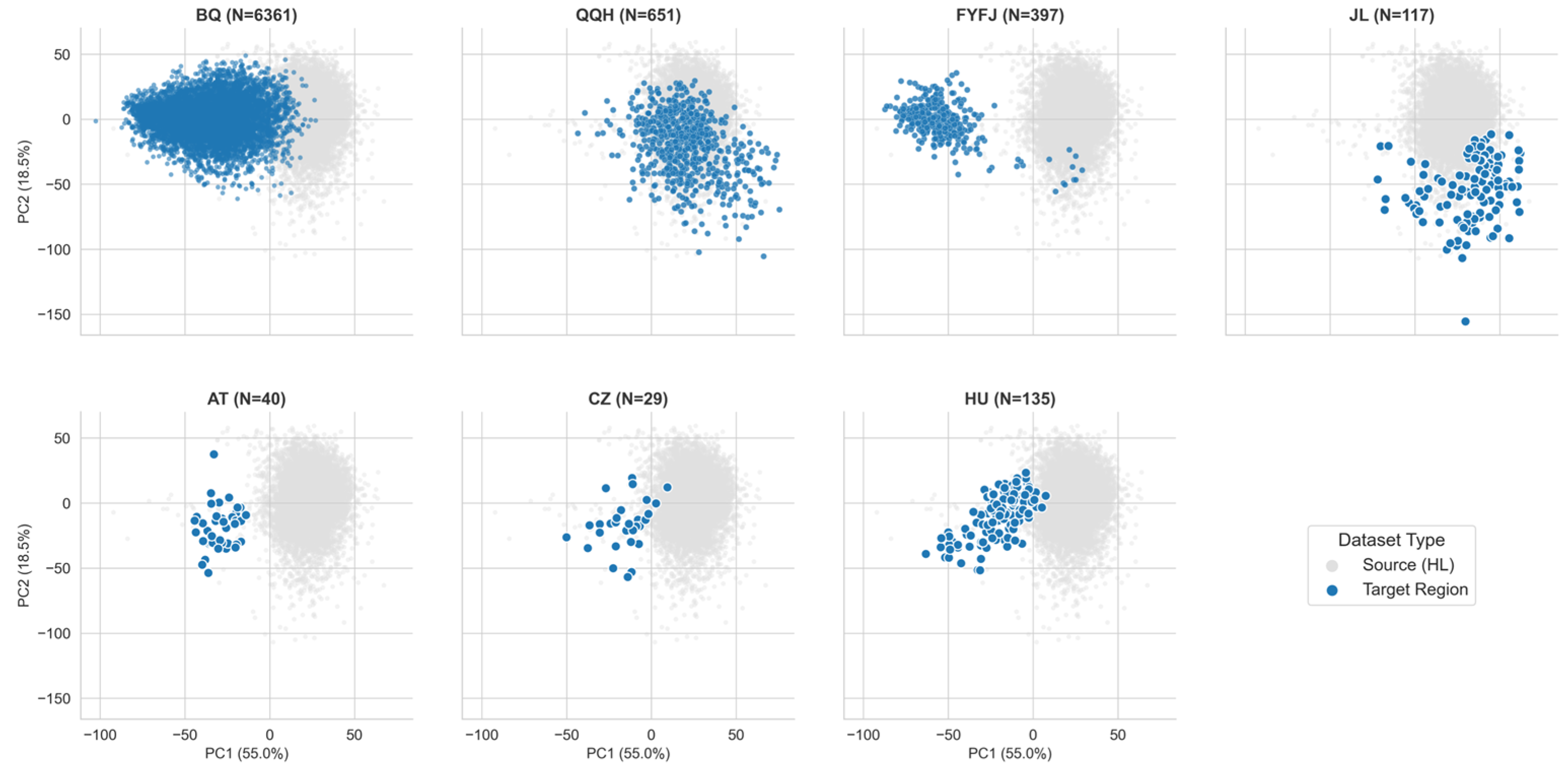
To evaluate the evolution of feature distributions before and after the extraction of SOC-OSFS, this study compared the PCA-derived spectral feature spaces of the full spectrum and the SOC-OSFS, as shown in Figure 5 and Figure 6. Based on the 401–2400 nm full-spectrum PCA projection (Figure 5), the HL samples (gray scatter points) exhibited a broad distribution centered around the origin in the feature space, forming a foundational data support with high coverage. In the subplots, the blue scatter points representing the validation regions displayed varying degrees of spatial shifting. The sample points of BQ and QQH highly overlapped with the HL background; however, FYFJ and JL shifted locally towards the negative axes of PC1 and PC2, respectively. In the European regions (AT, CZ, HU), which possess vastly different pedogenic environments, this phenomenon was even more pronounced, showing a significant systematic shift entirely towards the negative axis of the first principal component.
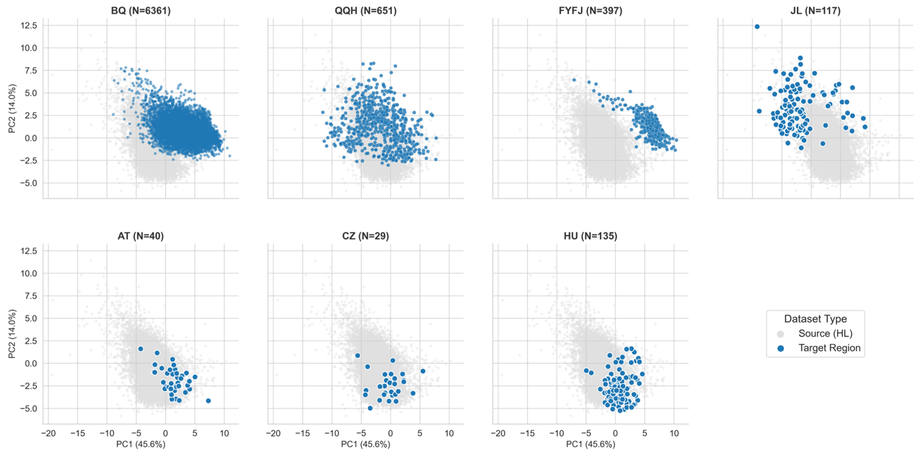
Compared to the full-spectrum PCA projection, the SOC-OSFS-based PCA projection (Figure 6) demonstrated a pronounced convergence trend. The overlap between the blue scatter points of the seven validation regions and the gray HL background increased remarkably. Most notably, the three European regions (AT, CZ, HU)—which previously exhibited the most severe deviation—shifted significantly closer to the center of the core study area. This phenomenon robustly demonstrates that extracting the SOC-OSFS effectively facilitates the realignment of spectral samples from diverse geographical regions within a low-dimensional feature space.

4.3.2. Cross-Regional Local Modeling Validation Using SOC-OSFS

To quantitatively assess the independent analytical capability of the SOC-OSFS across different regions, local prediction models were constructed for all eight study areas, with accuracy statistics presented in Table 2 (full evaluation metrics are detailed in Supplementary Table S1).
The results indicate that local models built upon the SOC-OSFS achieved stable predictive accuracies across all regions. In the Northeast China black soil regions with relatively abundant sample sizes, the models showed high goodness-of-fit, where the optimal CNN models for HL, QQH, and BQ all achieved an R 2 exceeding 0.88, while the optimal RF models for JL and FYFJ reached R 2 values of 0.8285 and 0.8360, respectively. In the European regions with limited sample sizes (AT, n = 40; CZ, n = 29; HU, n = 135), the SOC-OSFS-based RF models also demonstrated strong fitting performance, yielding R 2 values of 0.6714, 0.6876, and 0.7612, while constraining the RMSE to 0.337%, 0.363%, and 0.240%, respectively.

4.4. Evaluation of Cross-Regional Universal Prediction Method Based on SOC-OSFS

4.4.1. Model Prediction Results in the Core Study Area

This section compares the modeling performance of the full spectrum and SOC-OSFS in the HL region, as shown in Table 3.
Using full-spectrum data, the traditional PLSR and RF models achieved relatively stable fitting accuracies. Conversely, when processing 2000 high-dimensional variables, the deep learning models (CNN and LSTM) were hindered by redundant spectral information, resulting in accuracy metrics inferior to those of traditional models. When the input features were streamlined to the SOC-OSFS, the predictive performance of the CNN model was fully unleashed, achieving the optimal performance among the four models with its R 2 increasing to 0.8800 and RMSE decreasing to 0.1634. Although the full-spectrum PLSR model also exhibited high fitting accuracy ( R 2 = 0.8783), this was achieved at the cost of high model complexity associated with processing high-dimensional data. In contrast, the feature-selected CNN model maintained peak predictive accuracy utilizing only a minimal number of bands, further validating the efficacy of the SOC-OSFS as a robust foundation for cross-regional joint inversion.

4.4.2. Comparison of Cross-Regional Prediction Methods

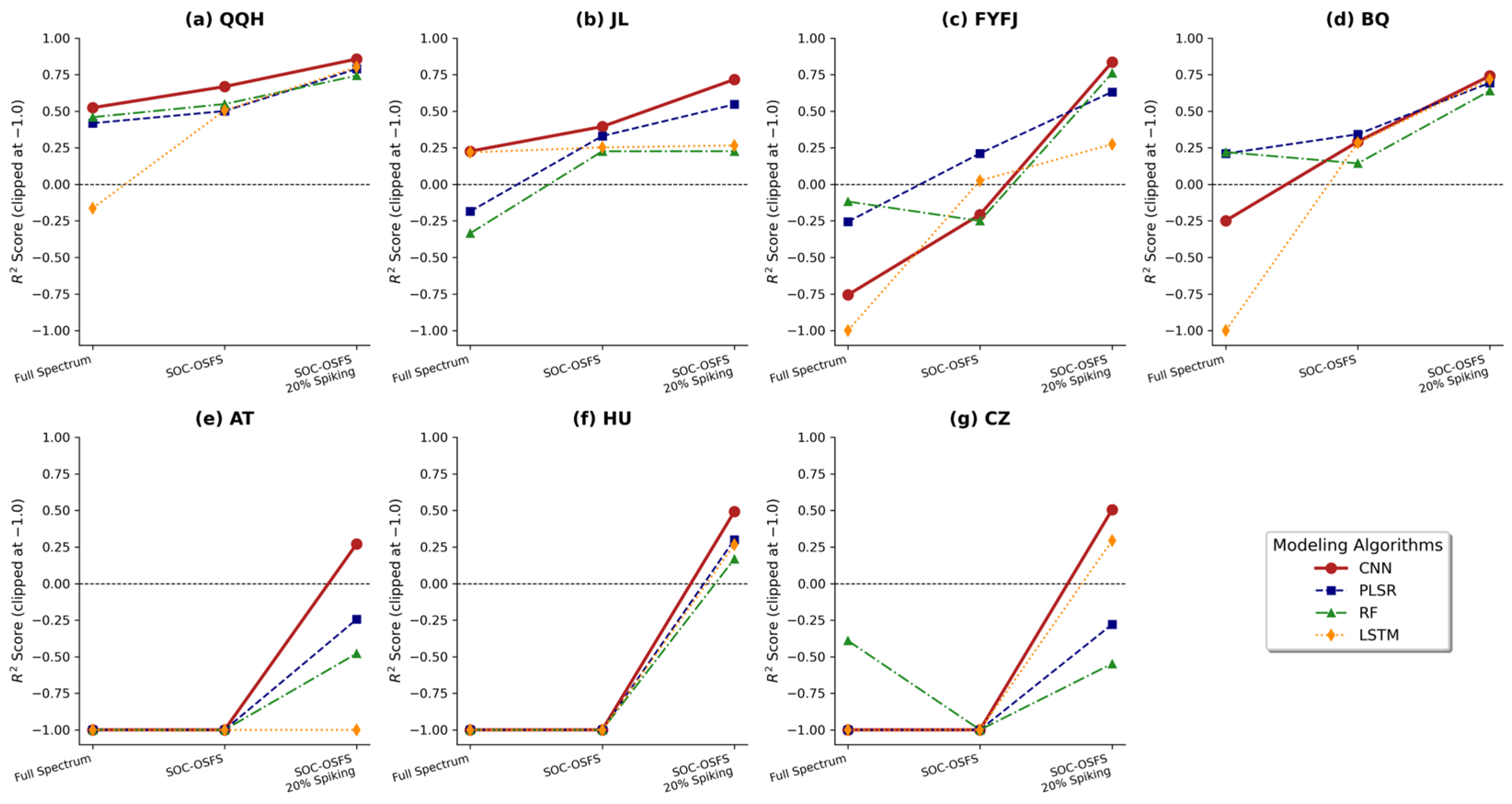
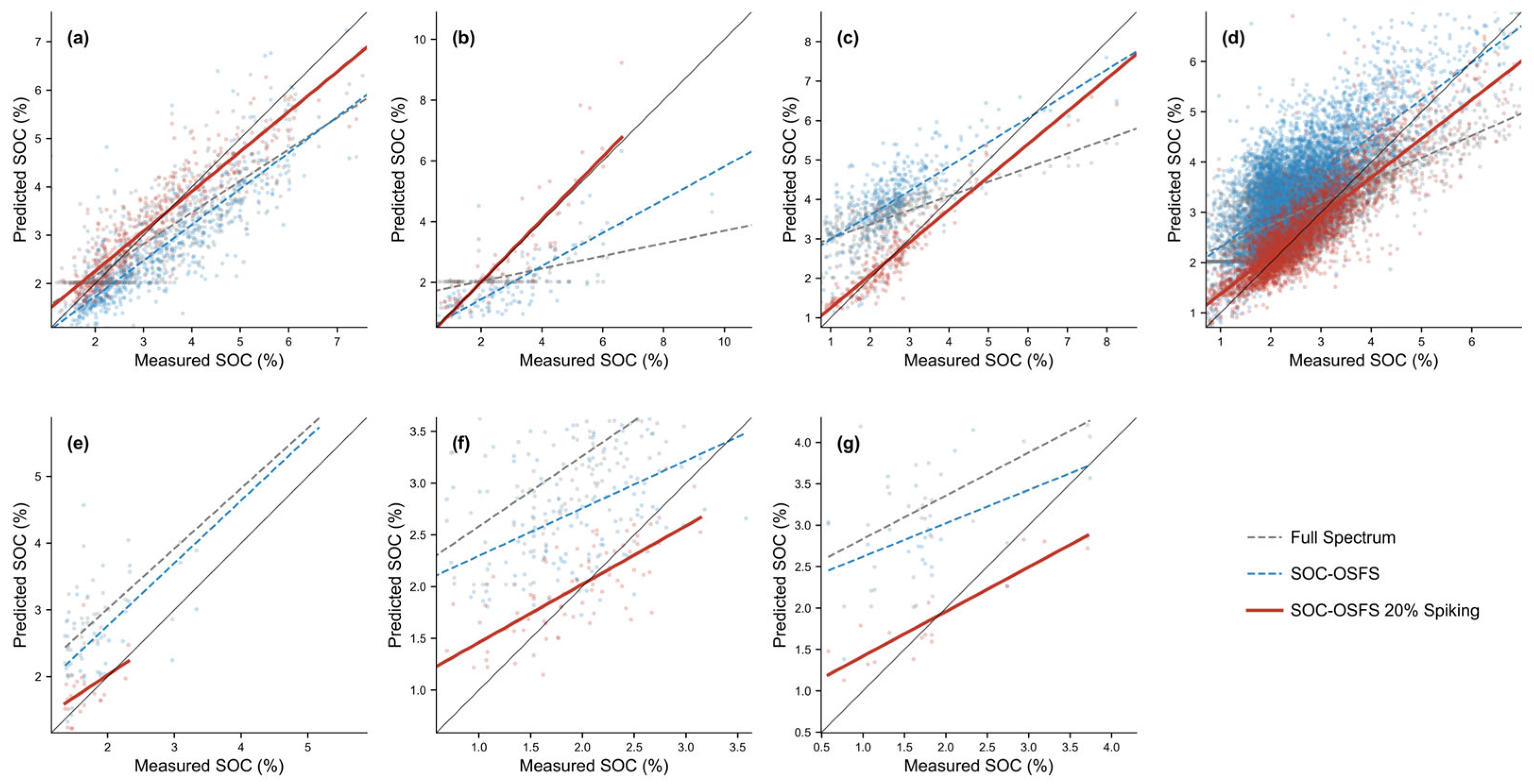
Using the CNN model as a representative example, this section compares the application effects of three strategies across the remaining seven independent validation regions: Full Spectrum Direct Prediction, SOC-OSFS Direct Prediction, and SOC-OSFS Combined with 20% Local Sample Spiking. To explicitly verify the statistical robustness of the predictions and assess the distributions of the 50 Monte Carlo simulations, paired-samples t-tests were conducted (complete statistical metrics for all models, including standard deviations, 95% confidence intervals, and exact p-values, are comprehensively documented in Supplementary Table S3). The model accuracy statistics are presented in Table 4 (complete metrics for other models are in Supplementary Table S2), and the evolutionary trajectories of model performance ( R 2 ) and the scatter distributions of predictions are illustrated in Figure 7 and Figure 8, respectively.
Initially, when applying the Full Spectrum Direct Prediction, model accuracies across all validation regions plummeted significantly. As shown in Figure 7, the starting points of the trajectories for this method were at extremely low levels. Particularly in the three European validation regions (AT, CZ, HU), the R 2 values for the full-spectrum models were entirely negative (Figure 7e–g). Observing the gray scatter points and dashed lines in Figure 8, the predicted values of the full-spectrum models deviated severely from the 1:1 reference line, exhibiting obvious systematic biases.
In contrast, utilizing the SOC-OSFS Direct Prediction yielded varying degrees of error reduction across all validation regions. Compared to the full-spectrum direct prediction approach, the R 2 trajectory of this proposed method shifted upward globally across all validation areas (Figure 7). For instance, in QQH, the R 2 improved from 0.5238 to 0.6684 (Table 4), and the RMSE decreased by over 15% in the vast majority of validation regions. In Figure 8, the blue dashed lines representing the SOC-OSFS direct prediction visibly converged towards the 1:1 ideality line compared to the gray dashed lines.
To further rectify the systematic intercept shifts in cross-regional predictions, this study introduced the SOC-OSFS 20% Spiking strategy. As demonstrated in Table 4 and Figure 7, under the guidance of a small volume of local sample data, predictive accuracy was drastically enhanced, displaying a distinct upward climbing trajectory. The fine-tuned CNN models achieved high goodness-of-fit in the Northeast China black soil regions, elevating the R 2 of QQH and FYFJ to 0.8567 and 0.8357, respectively (Table 4). As verified by the paired t-tests, the accuracy improvements achieved by the 20% spiking strategy were statistically highly significant (p < 0.01, denoted by ** in Table 4) across all target regions compared to the non-spiking strategies. Furthermore, as detailed in Table S3, the CNN model maintained extremely narrow 95% confidence intervals even in regions with smaller validation samples, quantitatively confirming the robust stability and reliability of its cross-regional estimations. In the European regions, this method successfully corrected the models back to positive linear fits. This accuracy improvement is especially intuitive in the scatter plots of Figure 8; the originally deviated fitting trajectories, after fine-tuning (red solid lines), became highly aligned with the 1:1 ideal reference line (black solid lines), and the convergence of the scatter distributions improved massively. Consequently, these results demonstrate that the SOC-OSFS combined with a minor local sample spiking strategy can effectively overcome the biases induced by geographical heterogeneity, realizing robust synergistic cross-regional SOC prediction.

5. Discussion

5.1. Physicochemical Mechanisms and Feature Space Realignment Underlying the Optimal Spectral Feature Set for SOC

This study constructed the optimal spectral feature set for soil organic carbon (SOC-OSFS) based on competitive adaptive reweighted sampling and the successive projections algorithm. The efficacy of this feature set is manifested not only in mathematical dimensionality reduction, but also in its robust support from explicit physicochemical response mechanisms.
As demonstrated in Section 4.2, the SOC-OSFS successfully reduced the full spectrum to merely 31 core bands (1.55% of the original dimensionality). The specific bands extracted in the visible region (e.g., 430, 433, and 447 nm) correspond directly to the electronic transitions of chromophores in humic substances. This result strongly aligns with the findings of Ben-Dor and Viscarra Rossel et al. [68], confirming that the feature set successfully captured the stable color-producing macromolecules formed during the evolution of black soil organic matter. Furthermore, key bands were selected in the SWIR-1 (1356 and 1406 nm) and SWIR-2 regions (e.g., 2197, 2220, and 2307 nm). These bands avoid the strong water absorption feature near 1400 nm. At the same time, they capture overtone responses of aliphatic C–H and N–H bonds in complex macromolecules such as lignin and cellulose. This spectral behavior is highly consistent with the classical mechanisms of soil organic matter absorption established by Stenberg et al. and Dalal & Henry [69,70].
Furthermore, it is worth noting that several selected bands (e.g., 696 nm, 1045 nm, and the cluster between 1820 nm and 1992 nm) fall outside these three primary highlighted intervals. Rather than representing direct organic absorption peaks, these additional bands were strategically retained by the SPA algorithm to serve as essential baseline anchors. Specifically, bands such as 696 nm and 1045 nm assist in mitigating the spectral interference from iron oxides and pedogenic parent materials [12], while the bands surrounding the 1900 nm region (e.g., 1820–1992 nm) are crucial for decoupling the dynamic background noise associated with soil moisture and clay minerals [29,48,69,71].
The purification of the aforementioned physicochemical mechanisms was intuitively corroborated during the actual cross-regional validation. When utilizing full-spectrum data, samples from diverse geographical regions exhibited severe deviations within the feature space. This is mainly because the full spectrum contains a large amount of non-target background information. These signals originate from soil parent materials, iron oxides, and clay minerals. Their strong spatial variability across regions masks the true spectral response of SOC. Conversely, when exclusively utilizing the optimal spectral feature set, samples from disparate geographical regions achieved a high degree of realignment within the feature space. This result demonstrates that extracting spectral response intervals with explicit physicochemical significance can effectively eliminate the interference of environmental background noise. This provides a novel perspective for research on feature band extraction in hyperspectral remote sensing inversion of SOC; namely, in future model construction, extracting such universal features can substantially mitigate the spatial heterogeneity issues induced by differences in pedogenic environments.

5.2. Application Potential of the Universal Cross-Regional Prediction Method

In the cross-regional prediction validation, full-spectrum models experienced severe accuracy degradation, or even complete failure, when applied to target domains with substantially different pedogenic environments. The root cause of this failure lies in the full-spectrum models’ severe overfitting to the specific soil matrices and redundant environmental variations in the core study area, thereby losing their spatial generalization capability [16,72]. In contrast, the optimal spectral feature set effectively reduced errors during direct cross-regional prediction, fully confirming its powerful filtering effect against environmental noise and its ability to preserve valid SOC spectral features that transcend geographical boundaries.
However, influenced by climate and long-term agricultural activities, different geographical units possess inherent intercept discrepancies in their background SOC concentrations; relying solely on feature extraction is insufficient to compensate for this systematic statistical shift. Validation results demonstrated that, building upon the optimal spectral feature set, introducing merely 20% of local samples for model fine-tuning (i.e., spiking) could elevate the predictive accuracy of each validation region to a level approaching that of independent local modeling [52,69]. This performance proves that the feature set possesses robust universality and plasticity in cross-regional predictions.
Overall, this cross-regional prediction framework shows strong practical potential. By establishing a foundational model based on the optimal spectral feature set, realizing high-accuracy spatial inversion in unknown geographical regions requires only the collection of a minimal number of field samples for local intercept correction. This approach drastically curtails the dense sampling costs required for large-scale predictions, offering a highly efficient solution for the large-scale remote sensing inversion and mapping of SOC.

5.3. Challenges and Limitations

Although the proposed method—combining the optimal spectral feature set with local sample fine-tuning—substantially improved cross-regional predictive accuracy, it still faces certain challenges in practical applications and subsequent mechanistic explorations.
First, in certain validation regions with extremely complex pedogenic backgrounds, the absolute accuracy of the fine-tuned models still has room for further improvement. Although the relatively small European validation sets were carefully selected for their pedological representativeness across Central Europe and exhibited statistical robustness in our uncertainty analysis, relying on limited cohorts inherently carries a risk of unstable estimations. In addition, potential temporal inconsistencies between datasets may introduce further uncertainty, although their impact is mitigated by the use of standardized laboratory measurement conditions. Future research could consider introducing samples covering a broader range of climate zones and soil types (such as expanding to more balanced European and Pan-Eurasian datasets) into the foundational dataset, evaluating a wider diversity of feature extraction and modeling algorithms, or employing advanced approaches that fuse neural network models with physical prior mechanisms, to further bolster the model’s capacity to represent spatial heterogeneity.
Second, this study was primarily conducted using laboratory hyperspectral data under ideal conditions; genuinely extrapolating this optimal spectral feature set to airborne or satellite-borne hyperspectral remote sensing platforms still necessitates overcoming complex external environmental interferences. In actual field remote sensing observations, factors such as soil surface roughness, dynamic variations in natural moisture content, crop residue coverage, and multiple atmospheric scatterings can all attenuate or even mask the faint spectral responses of SOC [73,74].

6. Conclusions

This study proposed and validated a cross-regional prediction method for soil organic carbon (SOC) based on an optimal spectral feature set, using datasets from the black soil regions of Northeast China and Europe. The primary conclusions are drawn as follows:
First, this study established the SOC-OSFS, which is supported by explicit physicochemical mechanisms. Based on CARS and SPA, a feature subset comprising 31 core bands was extracted from the full spectrum. Accounting for merely 1.55% of the original data dimensionality, this feature set precisely locked onto the spectral response intervals reflecting macromolecular functional groups such as humic chromophores, aliphatic C-H bonds, and N-H bonds. This feature set preserves key structural information while reducing interference from environmental moisture.
Second, this study confirmed the critical role of feature dimensionality reduction in decoupling environmental background noise and achieving spatial realignment. Full-spectrum data are highly susceptible to interference from non-target background signals such as iron oxides and clay minerals, which leads to significant shifts of cross-regional spectral samples within the feature space. However, based on the extracted optimal spectral feature set, black soil samples from diverse pedogenic backgrounds successfully overcame the impacts of geographical spatial differences and achieved feature space realignment, thereby mitigating the obstacles posed by spatial heterogeneity to the inversion models.
Finally, this study validated the cross-regional prediction method based on the optimal spectral feature set coupled with local sample correction. When encountering heterogeneous pedogenic environments, full-spectrum prediction models suffer from significant accuracy degradation due to overfitting to local data. In contrast, utilizing the optimal spectral feature set combined with intercept correction and model fine-tuning (spiking) using only 20% of local target samples can effectively overcome cross-regional prediction biases. This method elevated the predictive accuracy of each independent validation region to a level approaching that of independent local modeling, demonstrating excellent spatial generalization capability.
Overall, this study not only provides a novel perspective for resolving spatial heterogeneity issues in hyperspectral SOC inversion but also offers an effective method for large-scale SOC estimation. These findings provide a practical framework for large-scale SOC estimation and support future applications in digital soil mapping and carbon accounting using hyperspectral remote sensing. Future work should focus on improving model generalization by incorporating more diverse soil and climate datasets and further enhancing the transferability of laboratory-derived spectral features to satellite-scale applications.

Supplementary Materials

The following supporting information can be downloaded at: https://www.mdpi.com/article/10.3390/app16094433/s1, Table S1: Comprehensive evaluation metrics of local SOC prediction models using different algorithms based on the SOC-OSFS across all study regions; Table S2: Cross-regional prediction performances of the PLSR, RF, and LSTM models under three prediction strategies across the seven validation regions; Table S3: Statistical verification and uncertainty assessment of all four prediction models (CNN, PLSR, RF, and LSTM) under the 20% spiking strategy, based on 50-iteration Monte Carlo simulations.

Author Contributions

Conceptualization, A.Z. and S.C.; methodology, A.Z.; software, A.Z. and Z.W.; validation, A.Z., X.X. and Z.W.; formal analysis, A.Z.; investigation, A.Z., X.X. and Z.X.; resources, Z.X. and S.C.; data curation, A.Z. and Z.X.; writing—original draft preparation, A.Z.; writing—review and editing, S.C., X.X., Z.W. and Z.X.; visualization, A.Z.; supervision, S.C.; funding acquisition, S.C. All authors have read and agreed to the published version of the manuscript.

Funding

This research was funded by the Changchun Science and Technology Development Plan Project, the Major Science and Technology Special Project of the Changchun Satellite and Application Industry (Intelligent Evaluation of High-Precision Yield and Quality of Maize at the Plot Level Based on Integration of Satellite, Aerial, and Ground Data), grant number 2024WX06; the Seventh Batch of Jilin Province Youth Science and Technology Talents Support Program, grant number QT202322; and the Science and Technology Development Plan Project of Jilin Province, China, grant number YDZJ202401539ZYTS; the Science and Technology Research Project of the Education Department of Jilin Province, grant number JJKH20230344KJ. The APC was funded by grant number 2024WX06.

Institutional Review Board Statement

Not applicable.

Informed Consent Statement

Not applicable.

Data Availability Statement

The European black soil dataset analyzed in this study is publicly available in the LUCAS 2009 topsoil database (https://esdac.jrc.ec.europa.eu/content/lucas-2009-topsoil-data, accessed on 20 August 2023). The hyperspectral and SOC data from the Northeast China black soil regions presented in this study are available on request from the corresponding author. The data are not publicly available due to privacy restrictions related to ongoing research projects.

Acknowledgments

The authors would like to thank the Shenyang Geological Survey of China Geological Survey, China, and the Heilongjiang General Institute of Ecological Survey and Research, China, for providing the soil samples and SOC test data. We further acknowledge the Heilongjiang Provincial Geology and Mineral Resources Test and Application Institute, China, and the Liaoning Research Institute of Geology and Mineral Resources, China, for providing materials for part of the soil spectral measurements. Part of the spectral measurement work was supported by researchers from Jilin Jianzhu University, Changchun, China. Additionally, we would like to express our sincere gratitude to Menghan Wu, Yuqiao Suo, Yaqi Zhang, Jiaqi Yang, Jinchen Zhu, Qiqi Li, and Hao Chen for their valuable assistance and hard work in soil sample collection, laboratory spectral measurements, and data processing during this research.

Conflicts of Interest

The authors declare no conflicts of interest.

Abbreviations

The following abbreviations are used in this manuscript:
SOCSoil Organic Carbon
OSFSOptimal Spectral Feature Set
CARSCompetitive Adaptive Reweighted Sampling
SPASuccessive Projections Algorithm
PCAPrincipal Component Analysis
PLSRPartial Least Squares Regression
RFRandom Forest
CNNConvolutional Neural Network
LSTMLong Short-Term Memory
RMSERoot Mean Square Error
RPDRatio of Performance to Deviation

References

  1. Lin, H.; Duan, X.; Dong, Y.; Zhong, R.; Zheng, H.; Xie, Y.; Rong, L.; Zhao, H.; Wei, S. Soil inorganic carbon stock and its changes across the Tibetan Plateau during the 1980s–2020s. Glob. Planet. Change 2024, 236, 104433. [Google Scholar] [CrossRef] [Scilit]
  2. Xu, Z.; Chen, S.; Zhu, B.; Chen, L.; Ye, Y.; Lu, P. Evaluating the Capability of Satellite Hyperspectral Imager, the ZY1–02D, for Topsoil Nitrogen Content Estimation and Mapping of Farmlands in Black Soil Area, China. Remote Sens. 2022, 14, 1008. [Google Scholar] [CrossRef] [Scilit]
  3. Wiesmeier, M.; Urbanski, L.; Hobley, E.; Lang, B.; von Lützow, M.; Marin-Spiotta, E.; van Wesemael, B.; Rabot, E.; Liess, M.; Garcia-Franco, N.; et al. Soil organic carbon storage as a key function of soils—A review of drivers and indicators at various scales. Geoderma 2019, 333, 149–162. [Google Scholar] [CrossRef] [Scilit]
  4. Smith, P.; Soussana, J.F.; Angers, D.; Schipper, L.; Chenu, C.; Rasse, D.P.; Batjes, N.H.; Egmond, F.; McNeill, S.; Kuhnert, M.; et al. How to measure, report and verify soil carbon change to realize the potential of soil carbon sequestration for atmospheric greenhouse gas removal. Glob. Change Biol. 2020, 26, 219–241. [Google Scholar] [CrossRef] [Scilit] [PubMed]
  5. Ajami, M.; Heidari, A.; Khormali, F.; Gorji, M.; Ayoubi, S. Environmental factors controlling soil organic carbon storage in loess soils of a subhumid region, northern Iran. Geoderma 2016, 281, 1–10. [Google Scholar] [CrossRef] [Scilit]
  6. Hunter, B.D.; Roering, J.J.; Silva, L.C.R.; Moreland, K.C. Geomorphic controls on the abundance and persistence of soil organic carbon pools in erosional landscapes. Nat. Geosci. 2024, 17, 151–157. [Google Scholar] [CrossRef] [Scilit]
  7. Luo, C.; Kong, D.; Zhang, Y.; Bai, R.; Liu, H. Beyond decline: Spatial heterogeneity of soil organic matter as an emerging signal of cropland degradation in Northeast China. Catena 2026, 263, 109751. [Google Scholar] [CrossRef] [Scilit]
  8. Hein, C.J.; Usman, M.; Eglinton, T.I.; Haghipour, N.; Galy, V.V. Millennial-scale hydroclimate control of tropical soil carbon storage. Nature 2020, 581, 63–66. [Google Scholar] [CrossRef] [Scilit]
  9. Magalhães, L.P.d.; Sais, A.C.; Rossi, F. Research on Using Ensemble Models to Assess the Impacts of Climate Change on Agriculture Production: A Review. AgriEngineering 2025, 7, 219. [Google Scholar] [CrossRef] [Scilit]
  10. Meng, X.; Bao, Y.; Zhang, X.; Luo, C.; Liu, H. A long-term global Mollisols SOC content prediction framework: Integrating prior knowledge, geographical partitioning, and deep learning models with spatio-temporal validation. Remote Sens. Environ. 2025, 318, 114592. [Google Scholar] [CrossRef] [Scilit]
  11. Meng, X.; Bao, Y.; Luo, C.; Zhang, X.; Liu, H. SOC content of global Mollisols at a 30 m spatial resolution from 1984 to 2021 generated by the novel ML-CNN prediction model. Remote Sens. Environ. 2024, 300, 113911. [Google Scholar] [CrossRef] [Scilit]
  12. Viscarra Rossel, R.A.; Cattle, S.R.; Ortega, A.; Fouad, Y. In situ measurements of soil colour, mineral composition and clay content by vis–NIR spectroscopy. Geoderma 2009, 150, 253–266. [Google Scholar] [CrossRef] [Scilit]
  13. Bao, Y.; Meng, X.; Liu, H.; Xu, M.; Wang, M. A novel method for soil organic carbon prediction using integrated ‘ground-air-space’multimodal remote sensing data. Geoderma 2025, 460, 117453. [Google Scholar] [CrossRef] [Scilit]
  14. Gibson, A.J.; Hancock, G.R.; Bretreger, D.; Cox, T.; Hughes, J.; Kunkel, V. Assessing digital elevation model resolution for soil organic carbon prediction. Geoderma 2021, 398, 115106. [Google Scholar] [CrossRef] [Scilit]
  15. Wang, S.; Guan, K.; Zhang, C.; Lee, D.; Margenot, A.J.; Ge, Y.; Peng, J.; Zhou, W.; Zhou, Q.; Huang, Y. Using soil library hyperspectral reflectance and machine learning to predict soil organic carbon: Assessing potential of airborne and spaceborne optical soil sensing. Remote Sens. Environ. 2022, 271, 112914. [Google Scholar] [CrossRef] [Scilit]
  16. Padarian, J.; Minasny, B.; McBratney, A.B. Transfer learning to localise a continental soil vis-NIR calibration model. Geoderma 2019, 340, 279–288. [Google Scholar] [CrossRef] [Scilit]
  17. Röder, L.L.; Fischer, H. Theoretical investigation of applicability and limitations of advanced noise reduction methods for wavelength modulation spectroscopy. Appl. Phys. B Lasers Opt. 2022, 128, 10. [Google Scholar] [CrossRef] [Scilit]
  18. Rossel, R.A.V.; Webster, R. Predicting soil properties from the Australian soil visible-near infrared spectroscopic database. Eur. J. Soil Sci. 2012, 63, 848–860. [Google Scholar] [CrossRef] [Scilit]
  19. Jain, S.; Sethia, D.; Tiwari, K.C. A critical systematic review on spectral-based soil nutrient prediction using machine learning. Environ. Monit. Assess. 2024, 196, 699. [Google Scholar] [CrossRef] [Scilit] [PubMed]
  20. Moura-Bueno, J.M.; Dalmolin, R.S.D.; Ten Caten, A.; Dotto, A.C.; Demattê, J.A. Stratification of a local VIS-NIR-SWIR spectral library by homogeneity criteria yields more accurate soil organic carbon predictions. Geoderma 2019, 337, 565–581. [Google Scholar] [CrossRef] [Scilit]
  21. Guo, B.; Jin, G. Beyond the land quantity: Rethinking the role of land quality in agriculture from the efficiency perspective. Socio-Econ. Plan. Sci. 2025, 98, 102151. [Google Scholar] [CrossRef] [Scilit]
  22. Padarian, J.; Stockmann, U.; Minasny, B.; McBratney, A.B. Monitoring changes in global soil organic carbon stocks from space. Remote Sens. Environ. 2022, 281, 113260. [Google Scholar] [CrossRef] [Scilit]
  23. Yuan, J.; Cohen, M.J. Remote detection of ecosystem degradation in the Everglades ridge-slough landscape. Remote Sens. Environ. 2020, 247, 111917. [Google Scholar] [CrossRef] [Scilit]
  24. Guo, Y.; Ji, W.; Wu, H.; Shi, Z. Estimation and mapping of soil organic matter based on Vis-NIR reflectance spectroscopy. Spectrosc. Spectr. Anal. 2013, 33, 1135–1140. [Google Scholar] [CrossRef]
  25. Krishnan, P.; Alexander, J.D.; Butler, B.J.; Hummel, J.W. Reflectance Technique for Predicting Soil Organic Matter. Soil Sci. Soc. Am. J. 1980, 44, 1282–1285. [Google Scholar] [CrossRef] [Scilit]
  26. Xia, K.; Wu, T.; Zhang, S.; Wang, S.; Li, X.; Shen, Q.; Li, T. A new method for high-precision estimation of soil organic matter using two-dimensional correlation spectroscopy—To support collaborative use of global open soil spectral libraries. Geoderma 2024, 445, 116877. [Google Scholar] [CrossRef] [Scilit]
  27. Liu, J.; Xie, J.; Meng, T.; Dong, H. Organic matter estimation of surface soil using successive projection algorithm. Agron. J. 2022, 114, 1944–1951. [Google Scholar] [CrossRef] [Scilit]
  28. Li, Y.; Yang, X. Quantitative analysis of near infrared spectroscopic data based on dual-band transformation and competitive adaptive reweighted sampling. Spectrochim. Acta Part A Mol. Biomol. Spectrosc. 2023, 285, 121924. [Google Scholar] [CrossRef] [Scilit]
  29. Vohland, M.; Ludwig, B.; Seidel, M.; Hutengs, C. Quantification of soil organic carbon at regional scale: Benefits of fusing vis-NIR and MIR diffuse reflectance data are greater for in situ than for laboratory-based modelling approaches. Geoderma 2022, 405, 115426. [Google Scholar] [CrossRef] [Scilit]
  30. Zhong, X.; Zhao, L.; Wang, J.; Zheng, H.; Ren, P. Empirical models on urban surface emissivity retrieval based on different spectral response functions: A field study. Build. Environ. 2021, 197, 107882. [Google Scholar] [CrossRef] [Scilit]
  31. Dor, E.B.; Ong, C.; Lau, I.C. Reflectance measurements of soils in the laboratory: Standards and protocols. Geoderma 2015, 245–246, 112–124. [Google Scholar] [CrossRef] [Scilit]
  32. Kopačková, V.; Ben-Dor, E. Normalizing reflectance from different spectrometers and protocols with an internal soil standard. Int. J. Remote Sens. 2016, 37, 1276–1290. [Google Scholar] [CrossRef] [Scilit]
  33. Ma, Y.; Minasny, B.; Demattê, J.A.; McBratney, A.B. Incorporating soil knowledge into machine-learning prediction of soil properties from soil spectra. Eur. J. Soil Sci. 2023, 74, e13438. [Google Scholar] [CrossRef] [Scilit]
  34. Purushothaman, N.K.; Swan, T.; Singh, K.; Fidelis, C.; Majeed, I.; Yinil, D.; Minasny, B.; Das, B.S.; Field, D.J. Diffuse Reflectance Spectroscopy for Soil Testing Under Different Soil Nutrient Management in Cocoa Production Systems. Soil Use Manag. 2025, 41, e70094. [Google Scholar] [CrossRef] [Scilit]
  35. Odebiri, O.; Odindi, J.; Mutanga, O. Basic and deep learning models in remote sensing of soil organic carbon estimation: A brief review. Int. J. Appl. Earth Obs. Geoinf. 2021, 102, 102389. [Google Scholar] [CrossRef] [Scilit]
  36. Zhao, T.; Wang, S.; Ouyang, C.; Chen, M.; Liu, C.; Zhang, J.; Yu, L.; Wang, F.; Xie, Y.; Li, J. Artificial intelligence for geoscience: Progress, challenges, and perspectives. Innovation 2024, 5, 100691. [Google Scholar] [CrossRef] [Scilit]
  37. Minasny, B.; Bandai, T.; Ghezzehei, T.A.; Huang, Y.-C.; Ma, Y.; McBratney, A.B.; Ng, W.; Norouzi, S.; Padarian, J.; Sharififar, A. Soil science-informed machine learning. Geoderma 2024, 452, 117094. [Google Scholar] [CrossRef] [Scilit]
  38. Song, Q.; Zhang, W. Estimation and spatial distribution of soil organic carbon content in farmland using unmanned aerial vehicle hyperspectral remote sensing technology. Sci. Rep. 2026, 16, 5480. [Google Scholar] [CrossRef] [Scilit]
  39. Rizzo, R.; Wadoux, A.M.J.-C.; Demattê, J.A.M.; Minasny, B.; Barrón, V.; Ben-Dor, E.; Francos, N.; Savin, I.; Poppiel, R.; Silvero, N.E.Q.; et al. Remote sensing of the Earth’s soil color in space and time. Remote Sens. Environ. 2023, 299, 113845. [Google Scholar] [CrossRef] [Scilit]
  40. Carvalho, M.; Cardoso-Fernandes, J.; Lima, A.; Teodoro, A.C. Convolutional Neural Networks Applied to Antimony Quantification via Soil Laboratory Reflectance Spectroscopy in Northern Portugal: Opportunities and Challenges. Remote Sens. 2024, 16, 1964. [Google Scholar] [CrossRef] [Scilit]
  41. Zhang, Y.; Luo, C.; Zhang, W.; Wu, Z.; Zang, D. Mapping soil organic matter in Black Soil cropland areas using remote sensing and environmental covariates. Agriculture 2025, 15, 339. [Google Scholar] [CrossRef] [Scilit]
  42. Jiang, S.; Sweet, L.B.; Blougouras, G.; Brenning, A.; Li, W.; Reichstein, M.; Denzler, J.; Shangguan, W.; Yu, G.; Huang, F. How interpretable machine learning can benefit process understanding in the geosciences. Earth’s Future 2024, 12, e2024EF004540. [Google Scholar] [CrossRef] [Scilit]
  43. Wang, J.; Zou, Q.; Xu, B.; Feng, Z.; Yuan, H. Enhancing soil organic matter prediction via deep transfer learning from mid-infrared soil spectral library to in-situ field. Comput. Electron. Agric. 2026, 241, 111243. [Google Scholar] [CrossRef] [Scilit]
  44. Shen, Z.; Ramirez-Lopez, L.; Behrens, T.; Cui, L.; Zhang, M.; Walden, L.; Wetterlind, J.; Shi, Z.; Sudduth, K.A.; Baumann, P. Deep transfer learning of global spectra for local soil carbon monitoring. ISPRS J. Photogramm. Remote Sens. 2022, 188, 190–200. [Google Scholar] [CrossRef] [Scilit]
  45. Xu, Z.; Chen, S.; Lu, P.; Wang, Z.; Li, A.; Zeng, Q.; Chen, L. Optimizing a Standard Spectral Measurement Protocol to Enhance the Quality of Soil Spectra: Exploration of Key Variables in Lab-Based VNIR-SWIR Spectral Measurement. Remote Sens. 2022, 14, 1558. [Google Scholar] [CrossRef] [Scilit]
  46. Li, H.; Liang, Y.; Xu, Q.; Cao, D. Key wavelengths screening using competitive adaptive reweighted sampling method for multivariate calibration. Anal. Chim. Acta 2009, 648, 77–84. [Google Scholar] [CrossRef] [Scilit] [PubMed]
  47. Sanderman, J.; Baldock, J.A.; Dangal, S.R.S.; Ludwig, S.; Potter, S.; Rivard, C.; Savage, K. Soil organic carbon fractions in the Great Plains of the United States: An application of mid-infrared spectroscopy. Biogeochemistry 2021, 156, 97–114. [Google Scholar] [CrossRef] [Scilit]
  48. Clark, R.N.; King, T.V.V.; Klejwa, M.; Swayze, G.A.; Vergo, N. High spectral resolution reflectance spectroscopy of minerals. J. Geophys. Res. Solid Earth 1990, 95, 12653–12680. [Google Scholar] [CrossRef] [Scilit]
  49. Sanderman, J.; Baldock, J.A.; Amundson, R. Dissolved organic carbon chemistry and dynamics in contrasting forest and grassland soils. Biogeochemistry 2009, 89, 181–198. [Google Scholar] [CrossRef] [Scilit]
  50. Wold, S.; Esbensen, K.; Geladi, P. Principal component analysis. Chemom. Intell. Lab. Syst. 1987, 2, 37–52. [Google Scholar] [CrossRef] [Scilit]
  51. Timmerman, M.E. Principal Component Analysis. J. Am. Stat. Assoc. 2003, 98, 1082–1083. [Google Scholar] [CrossRef] [Scilit]
  52. Guerrero, C.; Wetterlind, J.; Stenberg, B.; Mouazen, A.M.; Gabarrón-Galeote, M.A.; Ruiz-Sinoga, J.D.; Zornoza, R.; Viscarra Rossel, R.A. Do we really need large spectral libraries for local scale SOC assessment with NIR spectroscopy? Soil Tillage Res. 2016, 155, 501–509. [Google Scholar] [CrossRef] [Scilit]
  53. Liu, B.; Guo, B.; Zhuo, R.; Dai, F. Estimation of soil organic carbon content by Vis-NIR spectroscopy combining feature selection algorithm and local regression method. Rev. Bras. Ciênc. Solo 2023, 47, e0230067. [Google Scholar] [CrossRef] [Scilit]
  54. IUSS Working Group. World Reference Base for Soil Resources 2014, Update 2015 International Soil Classification System for Naming Soils and Creating Legends for Soil Maps; IUSS Working Group: Rome, Italy, 2015. [Google Scholar]
  55. Walkley, A.; Black, I.A. An Examination of the Degtjareff Method for Determining Soil Organic Matter, and a Proposed Modification of the Chromic Acid Titration Method. Soil Sci. 1934, 37, 29–38. [Google Scholar] [CrossRef] [Scilit]
  56. DZ/T 0279.27-2016; Regional Geochemical Sample Analysis Methods—Part 27: Determination of Organic Carbon Content in Soil by Potassium Dichromate Oxidation Method. Ministry of Land and Resources of the People’s Republic of China: Beijing, China, 2016.
  57. Ben-Dor, E.; Patkin, K.; Banin, A.; Karnieli, A. Mapping of several soil properties using DAIS-7915 hyperspectral scanner data—A case study over clayey soils in Israel. Int. J. Remote Sens. 2002, 23, 1043–1062. [Google Scholar] [CrossRef] [Scilit]
  58. Xu, Z.; Chen, S.; Song, K. Black Soils Classification by Ground Spectral Process and Analysis. Acta Geol. Sin. (Engl. Ed.) 2019, 93, 152–157. [Google Scholar] [CrossRef] [Scilit]
  59. Pimstein, A.; Notesco, G.; Ben-Dor, E. Performance of Three Identical Spectrometers in Retrieving Soil Reflectance under Laboratory Conditions. Soil Sci. Soc. Am. J. 2011, 75, 746–759. [Google Scholar] [CrossRef] [Scilit]
  60. Panagos, P.; Van Liedekerke, M.; Jones, A.; Montanarella, L. European Soil Data Centre: Response to European policy support and public data requirements. Land Use Policy 2012, 29, 329–338. [Google Scholar] [CrossRef] [Scilit]
  61. Savitzky, A.; Golay, M.J.E. Smoothing and Differentiation of Data by Simplified Least Squares Procedures. Anal. Chem. 1964, 36, 1627–1639. [Google Scholar] [CrossRef] [Scilit]
  62. Demattê, J.A.M.; Dotto, A.C.; Paiva, A.F.S.; Sato, M.V.; Dalmolin, R.S.D.; de Araújo, M.d.S.B.; da Silva, E.B.; Nanni, M.R.; ten Caten, A.; Noronha, N.C.; et al. The Brazilian Soil Spectral Library (BSSL): A general view, application and challenges. Geoderma 2019, 354, 113793. [Google Scholar] [CrossRef] [Scilit]
  63. Wold, S.; Sjöström, M.; Eriksson, L. PLS-regression: A basic tool of chemometrics. Chemom. Intell. Lab. Syst. 2001, 58, 109–130. [Google Scholar] [CrossRef] [Scilit]
  64. Yan, Y.; Li, B.; Rossel, R.V.; Sun, F.; Huang, Y.; Shen, C.; Shi, Z.; Ji, W. Optimal soil organic matter mapping using an ensemble model incorporating moderate resolution imaging spectroradiometer, portable X-ray fluorescence, and visible near-infrared data. Comput. Electron. Agric. 2023, 210, 107885. [Google Scholar] [CrossRef] [Scilit]
  65. Belgiu, M.; Drăguţ, L. Random forest in remote sensing: A review of applications and future directions. ISPRS J. Photogramm. Remote Sens. 2016, 114, 24–31. [Google Scholar] [CrossRef] [Scilit]
  66. Hu, W.; Huang, Y.; Wei, L.; Zhang, F.; Li, H. Deep Convolutional Neural Networks for Hyperspectral Image Classification. J. Sens. 2015, 2015, 258619. [Google Scholar] [CrossRef] [Scilit]
  67. Greff, K.; Srivastava, R.K.; Koutnik, J.; Steunebrink, B.R.; Schmidhuber, J. LSTM: A search space odyssey. IEEE Trans. Neural Netw. Learn. Syst. 2017, 28, 2222–2232. [Google Scholar] [CrossRef] [Scilit] [PubMed]
  68. Ben-Dor, E. Quantitative Remote Sensing of Soil Properties. Adv. Agron. 2002, 75, 173–244. [Google Scholar] [CrossRef] [Scilit]
  69. Stenberg, B.; Rossel, R.A.V.; Mouazen, A.M.; Wetterlind, J. Visible and Near Infrared Spectroscopy in Soil Science. Adv. Agron. 2010, 107, 163–215. [Google Scholar] [CrossRef] [Scilit]
  70. Dalal, R.C.; Henry, R.J. Simultaneous Determination of Moisture, Organic Carbon, and Total Nitrogen by Near Infrared Reflectance Spectrophotometry. Soil Sci. Soc. Am. J. 1986, 50, 120–123. [Google Scholar] [CrossRef] [Scilit]
  71. Nawar, S.; Buddenbaum, H.; Hill, J.; Kozak, J.; Mouazen, A.M. Estimating the soil clay content and organic matter by means of different calibration methods of vis-NIR diffuse reflectance spectroscopy. Soil Tillage Res. 2016, 155, 510–522. [Google Scholar] [CrossRef] [Scilit]
  72. Brown, D.J. Using a global VNIR soil-spectral library for local soil characterization and landscape modeling in a 2nd-order Uganda watershed. Geoderma 2007, 140, 444–453. [Google Scholar] [CrossRef] [Scilit]
  73. Nocita, M.; Stevens, A.; van Wesemael, B.; Aitkenhead, M.; Bachmann, M.; Barthès, B.; Dor, E.B.; Brown, D.J.; Clairotte, M.; Csorba, A.; et al. Soil Spectroscopy: An Alternative to Wet Chemistry for Soil Monitoring. Adv. Agron. 2015, 132, 139–159. [Google Scholar] [CrossRef] [Scilit]
  74. Chabrillat, S.; Ben-Dor, E.; Cierniewski, J.; Gomez, C.; Schmid, T.; van Wesemael, B. Imaging Spectroscopy for Soil Mapping and Monitoring. Surv. Geophys. 2019, 40, 361–399. [Google Scholar] [CrossRef] [Scilit]
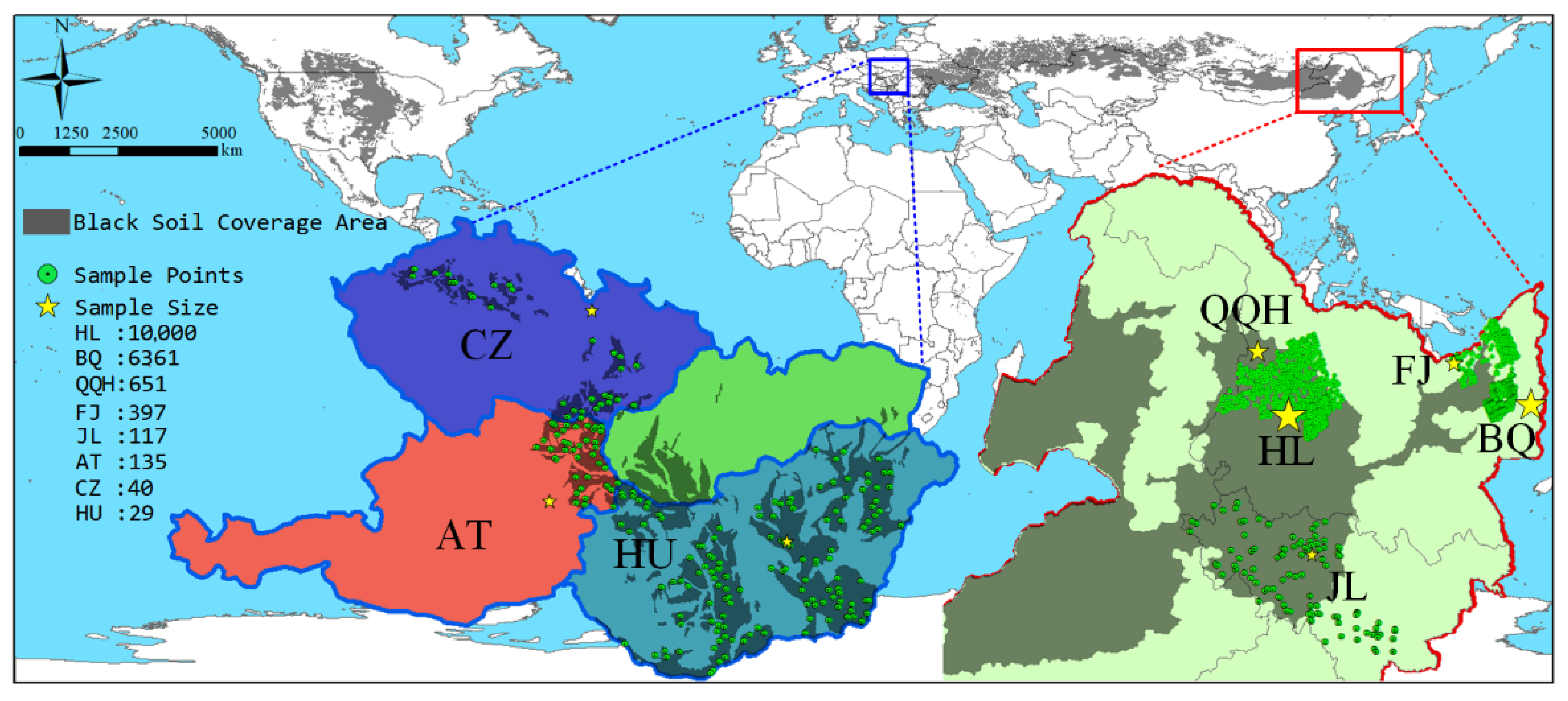
Figure 1. Spatial distribution of sampling points across the eight black soil target domains in the Eurasian continent. The red and blue boxes and lines indicate the geographic extents of the Northeast China and European black soil study regions, respectively.
Applsci 16 04433 g001
Figure 2. Performance evaluation of PLSR and RF models using different spectral transformation forms in the core study area (HL).
Applsci 16 04433 g002
Figure 3. Feature selection process based on the hybrid CARS-SPA method. (a) The CARS selection process, where the red dot represents the optimal variable subset with the minimum RMSECV; (b) The SPA selection process, where the red dot indicates the optimal elbow point.
Applsci 16 04433 g003
Figure 4. Distribution of the SOC-OSFS characteristic bands on the mean spectral curve of black soils. The solid gray line represents the mean reflectance spectrum of black soil samples in the source domain (HL); the red dots indicate the locations of the 31 bands in the SOC Optimal Spectral Feature Set (SOC-OSFS); the colored background areas represent the characteristic response regions closely related to soil organic carbon in the visible (Vis), shortwave near-infrared (SWIR-1), and longwave near-infrared (SWIR-2) domains.
Applsci 16 04433 g004
Figure 5. Spatial distribution of full-spectrum features across different black soil regions.
Applsci 16 04433 g005
Figure 6. Spatial distribution of SOC-OSFS features across different black soil regions.
Applsci 16 04433 g006
Figure 7. Performance trajectories of SOC prediction ( R 2 ) across verification regions under three cross-regional prediction methods. Subplots (ag) represent different target regions: (a) QQH, (b) JL, (c) FYFJ, (d) BQ, (e) AT, (f) HU, and (g) CZ. The x-axis denotes three prediction methods: Full Spectrum Direct, SOC-OSFS Direct, and SOC-OSFS 20% Spiking. Different colors and line styles indicate various algorithms: Red solid line for CNN; Blue dashed line for PLSR; Green dash-dot line for RF; and Orange dotted line for LSTM. The black horizontal dashed line represents the reference baseline at R2 = 0.
Applsci 16 04433 g007
Figure 8. Scatter plots and linear regression comparisons of measured versus predicted SOC across verification regions. Subplots (ag) correspond to the same regions as in Figure 7. Gray, blue, and red scatters and their corresponding regression lines represent the Full Spectrum Direct, SOC-OSFS Direct, and SOC-OSFS Spiking prediction methods, respectively. Their corresponding linear regression fits are shown as gray dashed, blue dashed, and red solid lines. The solid black line represents the 1:1 ideal reference line.
Applsci 16 04433 g008
Table 1. Descriptive statistics of soil organic carbon (SOC) content for the source and target domains.
ClassificationRegionNMin (%)Max (%)Mean (%)SD (%)CV (%)Skewness
Source DomainHL10,0000.178.82.510.728.091.24
CN RegionsBQ63610.4120.32.61.0339.592.7
QQH6510.957.973.181.2840.280.79
FYFJ3970.6711.452.561.2247.692.66
JL1170.4212.592.811.8365.211.96
EU RegionsHU1350.553.581.960.5829.79−0.07
AT401.365.171.90.7137.162.91
CZ290.583.741.840.7842.560.94
Table 2. Performance of optimal local prediction models across regions based on SOC-OSFS.
RegionNBest ModelR2RMSE (%)
HL10,000CNN0.880.1634
QQH 651CNN0.88530.431
JL118RF0.82850.659
FYFJ397RF0.83600.513
BQ6361CNN0.88540.459
HU135RF0.76120.24
CZ29RF0.68760.363
AT40RF0.67140.337
Table 3. Comparison of modeling accuracy between full-spectrum and SOC-OSFS in the core study area (HL).
ModelFeatureR2RMSE (%)RPDBias
CNNSOC-OSFS0.88000.16342.88680.0257
CNNFull-Spectrum0.80280.24452.2521−0.0813
LSTMSOC-OSFS0.86740.17182.74640.0044
LSTMFull-Spectrum0.86780.20022.75080.0172
PLSRSOC-OSFS0.81690.20192.33680.032
PLSRFull-Spectrum0.87830.19212.86630.0277
RFSOC-OSFS0.87320.1682.80870.0125
RFFull-Spectrum0.87640.19362.84450.011
Table 4. Performance comparison of the representative model (CNN) across verification regions under three cross-regional prediction methods.
RegionMetricsFull SpectrumSOC-OSFSSOC-OSFS
20% Spiking
QQHR20.52380.66840.8567 **
RMSE (%)0.88380.73750.4791 **
FYFJR2−0.7559−0.20700.8357 **
RMSE (%)1.61761.34110.4659 **
BQR2−0.24890.29180.7419 **
RMSE (%)1.15040.86620.5270 **
JLR20.22640.39460.7170 **
RMSE (%)1.60461.41950.7831 **
CZR2−3.2861−2.51640.5051 **
RMSE (%)1.59561.44530.5242 **
HUR2−4.7995−2.11260.4919 **
RMSE (%)1.40081.02620.4111 **
ATR2−1.5917−1.12440.2715 **
RMSE (%)1.12271.01640.3920 **
Note: The reported values are the robust means derived from 50-iteration Monte Carlo simulations. The asterisks (**) denote that the performance improvement achieved by the 20% spiking strategy is statistically highly significant (p < 0.01) compared to the non-spiking strategies, based on paired-samples t-tests.
Disclaimer/Publisher’s Note: The statements, opinions and data contained in all publications are solely those of the individual author(s) and contributor(s) and not of MDPI and/or the editor(s). MDPI and/or the editor(s) disclaim responsibility for any injury to people or property resulting from any ideas, methods, instructions or products referred to in the content.