An LSTM Autoencoder-Based Approach for Monitoring Railway Bridges

Abstract

Continuous monitoring of railway bridges is essential for ensuring safety and operational reliability, considering aging mechanisms, rising traffic, and elevated speeds of railway vehicles. Frequently, traditional vibration-based approaches, including modal identification and data-driven diagnostic strategies, are strongly influenced by environmental and operational variability, requiring labeled damaged datasets or numerical simulations to provide reliable outcomes. However, the acquisition of complete and representative datasets for training neural networks in structural health monitoring remains a challenging task, particularly for large-scale civil structures such as bridges. In these cases, unsupervised learning approaches represent promising solutions. An unsupervised anomaly detection methodology for railway bridge monitoring based on a long short-term memory (LSTM) autoencoder (AE) trained exclusively on bridge accelerations under healthy structural conditions is proposed in the present work. Specifically, the acceleration responses are obtained from simulations made on a calibrated finite element model of the bridge, reproducing realistic train–bridge interaction scenarios. The multi-channel acceleration signals are reconstructed by the proposed LSTM AE to produce the Root Mean Square Error (RMSE) between measured and reconstructed acceleration responses as indicators of potential structural anomalies. A dual-threshold strategy is adopted for damage detection purposes, including a global threshold for identifying anomalies in the overall dynamic response and per-sensor thresholds derived from the healthy-condition RMSE distribution for detecting localized damages. Only healthy-condition data are required for employing the proposed technique, avoiding labeled damaged data for training purposes. The LSTM AE constitutes an effective and computationally efficient tool for anomaly detection and continuous structural health monitoring of railway bridges, as demonstrated by the obtained results, representing a promising alternative to classical modal-based approaches and existing deep learning-based methods.

1. Introduction

Railway bridges are essential components of transportation networks; nowadays they are subjected to increasing traffic, growing dynamic loads and traveling speeds [1]. These factors, combined with aging processes, threaten the structural integrity, safety and operability of the railway network. In this critical context, structural health monitoring (SHM) represents a fundamental tool for assessing structural conditions, planning maintenance activities and supporting life-cycle management strategies [2,3,4,5,6].

In the last few decades, SHM has gained growing interest in supporting and complementing traditional inspection procedures, typically based on visual surveys and periodic manual assessments, which are characterized by significant limitations and shortcomings [7], mainly related to their intrinsic subjectivity, inability to detect incipient or localized deterioration phenomena and the discretized frequency. Conversely, vibration-based SHM approaches potentially allow for quantitatively and continuously monitoring structural behavior. This can be achieved through the deployment of different sensing devices, such as accelerometers, velocimeters, linear variable displacement transducers (LVDTs), and fiber-optic sensors, among others. This, in practice, allows the extraction of dynamic (or static) indicators of structural integrity under in-service operational conditions [8,9,10].

Within vibration-based SHM, Operational Modal Analysis (OMA) has emerged as a central methodology for extracting modal parameters from structural response under operational and environmental actions [11]. Several studies have demonstrated the capability of OMA procedures, including covariance-driven stochastic subspace identification (SSI-COV), enhanced frequency domain decomposition (EFDD), transmissibility-based identification, and hybrid deterministic–stochastic techniques, to provide robust modal tracking even under challenging environmental and operational conditions [12,13]. These approaches have been successfully applied to steel truss bridges, reinforced concrete structures, arch bridges, and long-span cable-stayed systems, demonstrating effectiveness in long-term monitoring and in improving the interpretation of dynamic responses collected over extended time periods [14,15,16,17,18,19,20]. In fact, since modal parameters, i.e., natural frequencies and associated mode shapes and damping ratios, are related to structural condition [21,22], their tracking over time allows for an evaluation of the status of the monitored structure. However, it is well known that the natural frequencies of a bridge structure may be largely influenced by environmental factors, such as temperature and humidity [3,5,23]. Moreover, the reduced sensitivity to local damages may limit the early damage detection capability of modal-based indicators.

In recent years, machine learning (ML) and deep-learning techniques applied to SHM for railway bridges have been increasingly adopted to overcome the limitations of modal approaches [24,25]. Several works have explored drive-by (even called train-borne) detection methodologies, in which convolutional neural networks (CNNs) are trained on simulated or measured vehicle responses to identify structural damage indirectly through bogie accelerations [26]. Hybrid deep learning architectures, such as 1D-CNNs combined with Recurrent Neural Networks (RNNs), have been introduced in [21,26] to exploit synthetic datasets generated from calibrated finite element models to classify single or multiple damage scenarios. Additional developments include regression-based ML models for long-term monitoring using environmental and static measurements [23], digital-twin frameworks integrating vibration data with anomaly detection algorithms [27], and neural network-based methodologies relying on Gaussian processes, shallow ANNs, CNNs, or residual networks for predicting healthy accelerations and identifying deviations associated with structural deterioration [24,28,29,30,31].

Another form of proposed anomaly detection techniques is constituted of unsupervised ones. Algorithms such as one-class support vector machines, isolation forests, local outlier factor, and robust random cut forest have been adopted in several studies, demonstrating reliability in detecting abrupt changes through strain and acceleration features [32,33]. Other unsupervised approaches feature the use of statistical techniques such as Extreme Value Theory [34], autoencoders [35,36], and DBSCAN paired with spectral clustering [37]. Several technical challenges still limit the effectiveness of existing approaches, although improvements have been made in the field of vibration-based structural health monitoring. Structural responses are strongly influenced by environmental and operational variability, which can mask or mimic damage-induced changes. Furthermore, many machine learning techniques are based on labeled datasets, including both healthy and damaged conditions, which are rarely available for real bridge structures. Finally, classical modal-based approaches exhibit limited sensitivity to localized damage, making early detection particularly challenging. Despite the previously mentioned promising results, most existing approaches exhibit limitations such as reliance on simulated datasets rather than long-term field measurements, and limited generalization capability to changing operational conditions. Unsupervised reconstruction-based strategies capable of learning the intrinsic dynamics of the healthy structure and detecting damage through deviations from the learned behavior have been explored in a limited number of works. These approaches are inherently well-suited for SHM applications, where structural responses are influenced by complex phenomena such as environmental fluctuations, train–bridge interaction, multi-modal vibration patterns, and sensor noise [32]. Moreover, given their nature, they overcome the limitations of requiring a comprehensive dataset referring to the damaged states of the structure.

The present work proposes an unsupervised SHM methodology for railway bridges based on a long short-term memory (LSTM) autoencoder (AE), trained exclusively on multi-sensor numerical acceleration time histories, referring to healthy structural conditions. Precisely, bridge accelerations are evaluated at the nodes of the FE model corresponding to the actual positions of the velocimeters installed on the actual structure.

The LSTM AE reconstructs the entire set of accelerations by exploiting temporal dependencies and spatial correlations related to bridge structural dynamic behavior. Deviations between measured and reconstructed signals are quantified through the root mean square error (RMSE), computed on ten-second time windows, enabling the identification of anomalous behaviors, a potential indication of the occurrence of structural damage.

Two complementary strategies were developed to enhance detection performance. A global window-level threshold, based on the distribution of healthy-condition reconstruction errors, is adopted to identify anomalies affecting the overall dynamic response. Moreover, per-sensor thresholds, defined according to the classical three-sigma statistical rule [38,39], are applied to the RMSE distribution concerning each sensor, enhancing sensitivity to localized damage. The proposed framework combines the advantages of deep learning, reconstruction-based anomaly detection, and multi-sensor response analysis, providing a data-driven, yet physically consistent tool for continuous monitoring of railway bridges under realistic operating scenarios simulated through a calibrated numerical model.

The main contributions of the present work can be summarized as follows:

• An unsupervised SHM methodology based on an LSTM-based autoencoder, trained exclusively on healthy-condition acceleration data, capable of detecting both global and localized structural anomalies without requiring labeled damaged datasets;
• A reconstruction-based damage indicator, defined through the RMSE, which allows for detecting subtle variations in the structural behavior that may not be reflected in modal parameter changes or frequency-based metrics;
• A dual-threshold anomaly detection strategy, including a global window-level threshold and sensor-specific thresholds derived from healthy-condition error distributions, which enhances sensitivity to localized deterioration while preserving robustness against environmental and operational variability;
• A methodology providing a complementary data-driven framework for attempting to mitigate limitations of OMA and supervised ML approaches, particularly in scenarios where labeled damage data are not available.

To better position the proposed methodology within the current literature, a structured comparison with recent deep learning-based approaches for structural health monitoring (SHM) is provided. While studies based on LSTM, autoencoder (AE), and graph-based architectures have shown promising capabilities for damage detection, significant differences remain regarding data requirements, model complexity, and evaluation settings.

Specifically, LSTM-based approaches, such as [40], typically rely on supervised learning and require labeled damage datasets, often focusing on indirect measurements derived from vehicle–bridge interactions. In contrast, the framework presented here is fully unsupervised and utilizes direct multichannel bridge accelerations. Regarding autoencoder-based methods, works such as [41] employ reconstruction-based anomaly detection using vehicle-based responses in a drive-by setup, which offers limited spatial exploitation; our approach instead utilizes direct monitoring to enable explicit spatial-temporal modeling. While ref. [42] explores comparative AE methods for general SHM, the present study is specifically tailored to railway bridges by leveraging LSTM-driven temporal modeling. Furthermore, although the method in [43] provides near real-time anomaly detection using numerical and experimental data on generic structures, it lacks a refined validation scheme. The current framework addresses this by incorporating a dual-threshold approach—combining global and per-sensor thresholds—to improve detection sensitivity and localization. Finally, while graph-based methods like those in [44] can explicitly model spatial relations via Graph Neural Networks (GNNs), they generally necessitate high architectural complexity and large, structured datasets. Compared to these approaches, the proposed methodology adopts a more streamlined LSTM-autoencoder architecture. It remains fully unsupervised, training exclusively on healthy-condition accelerations, and effectively exploits multichannel temporal data without the computational overhead of graph-based modeling.

The remaining part of the paper is organized as follows: Section 2 describes the case study under analysis. Subsequently, in Section 3, the attention is focused on the description of the finite element model of the bridge adopted in this work. The AI-based framework, developed for anomaly detection purposes, is described in Section 4. Section 5 shows and describes the results obtained from simulations, analyzing the performance of the proposed methodology. Finally, conclusions and future perspectives are discussed in Section 6.

2. Case Study

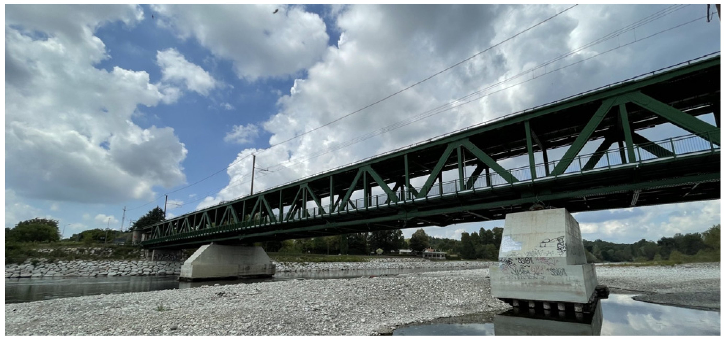
The bridge under study spans the Ticino River, located in the municipality of Turbigo, between the cities of Turbigo and Galliate in northern Italy. It was built in 1952 to replace an older structure, damaged after World War II.

The bridge, shown in Figure 1, features a steel truss girder design with four supports, all made of reinforced concrete. The lateral supports rest on two box abutments located on both sides of the river, while the central supports are positioned on two piers within the river. The structure has two decks: the upper deck serves as a railway line (single track), made entirely of steel. Instead, the lower deck is designated for road vehicles (with two lanes) and includes two lateral steel grillages for pedestrian use. The bridge span is divided into three sections: 44 m on Galliate’s side, 56 m for the mid-span, and 45 m on Turbigo’s side. Additionally, the bridge incorporates two Gerber connections in the mid-span, both located at one-fifth of the span length.

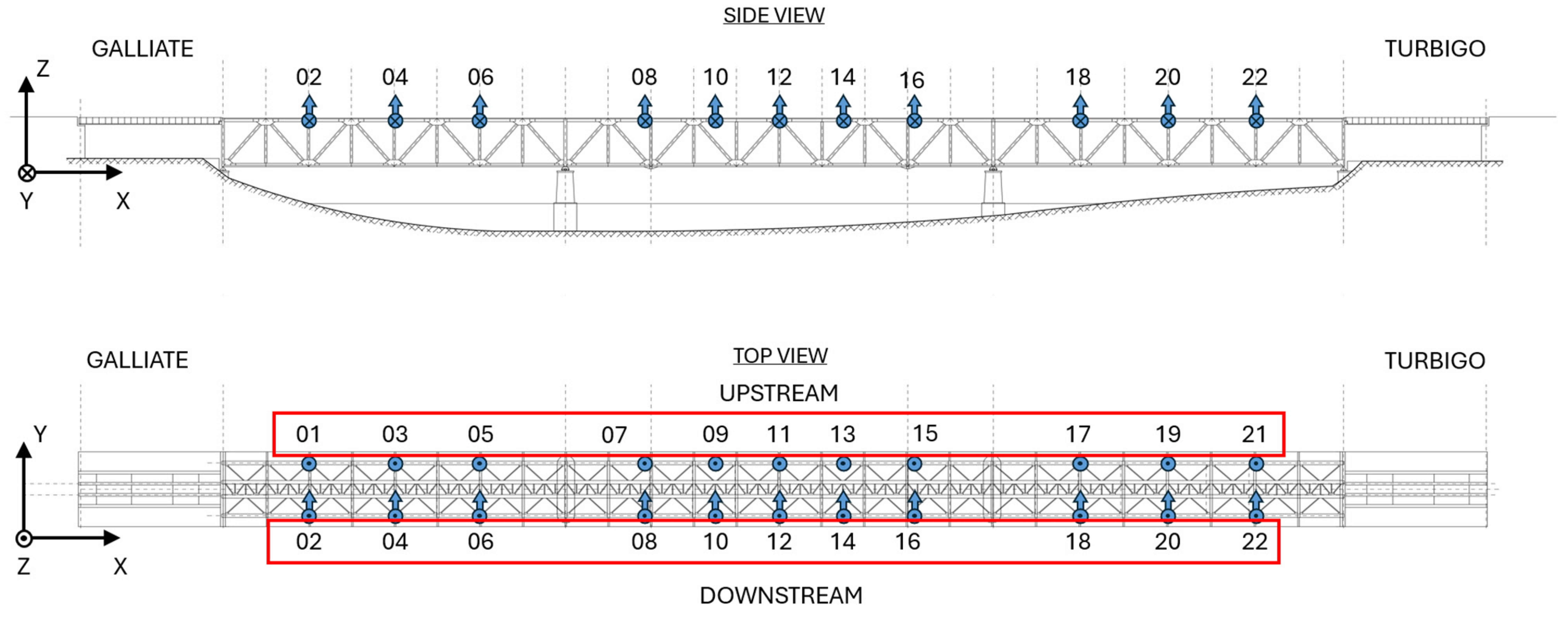
The monitoring system installed on this railway bridge is composed, among the others, of twenty-two velocimeters (i.e., SARA SS45) dedicated to measuring vertical velocities along the vertical axis (z), promptly converted into accelerations. The sensors are distributed along the longitudinal axis (x) of the deck and arranged into two parallel rows corresponding to the upstream and downstream sides of the structure, as schematically depicted in Figure 2.

Each sensor is mounted directly onto the main longitudinal upper girders, providing a homogeneous sampling of the vertical response along the span. The top view emphasizes the spatial organization of the sensing grid: odd-indexed sensors (IDs 01–21) are located on the upstream side of the deck, whereas even-indexed sensors (IDs 02–22) are aligned downstream. It is important to notice that only sensors installed on the downstream side of the bridge acquire data along the lateral direction (y-axis). A dense spatial discretization of the vertical dynamic response is ensured by the presented configuration, enhancing the monitoring system to detect both global and localized changes in structural behavior, including potential asymmetries between the two sides of the deck.

The complete sensor array potentially enables the proposed Artificial Intelligence (AI)-based methodology for anomaly detection tasks. The multi-sensor layout, combined with its symmetric deployment, provides a reliable basis for identifying deviations from the healthy structural state. In this paper, numerical accelerations refer to the nodes located in correspondence with the sensors mounted on the actual structure.

3. Models

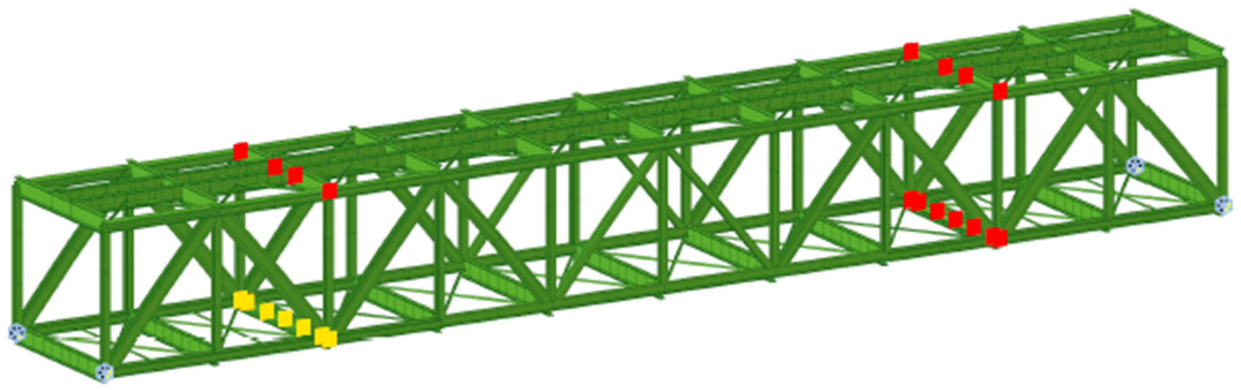
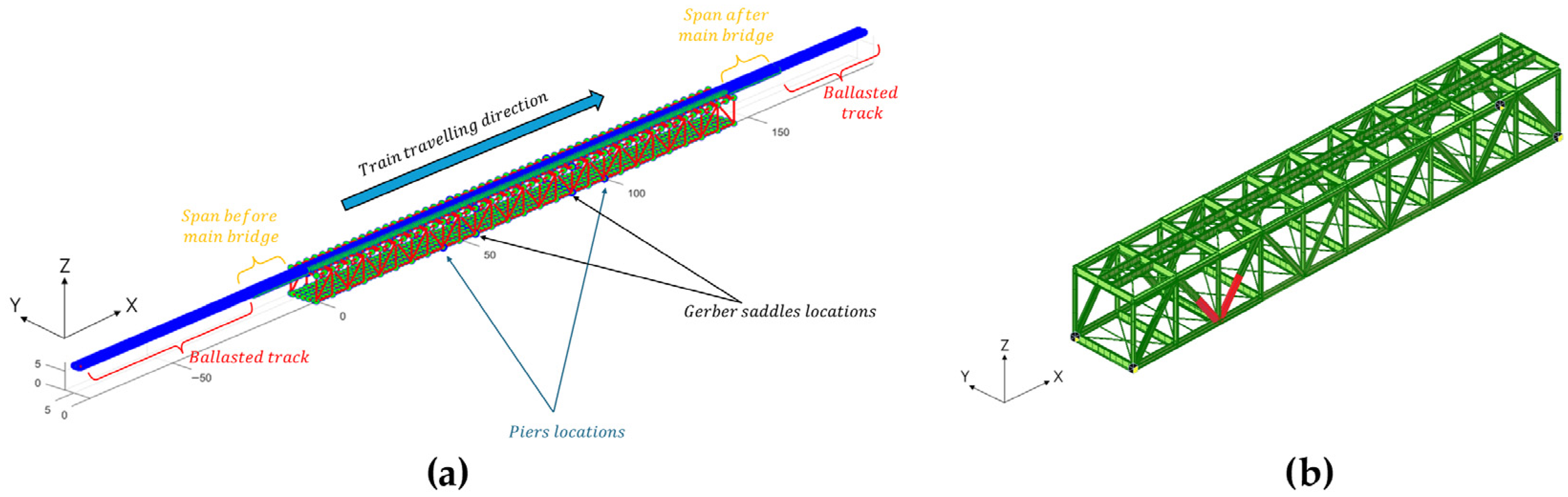
To accurately simulate the response of the bridge, a calibrated FE model was designed, shown in Figure 3a. This step is crucial, as the accuracy of subsequent damage simulations depends on the reliability and representativeness of the model. The modeling process consisted of two steps: an initial modeling phase, during which the primary assumptions and structural properties are defined, and a calibration phase, where the model parameters are refined and tuned to closely match the actual behavior of the bridge.

Two structural analysis software were used in this work, i.e., Midas GEN 2025 v1.2 and ADTreS [45]. The first is used to create the initial model of the bridge, incorporating its geometry and structural properties. This stage relied on technical drawings created as part of the most recent studies and subsequent interventions. Later, the model was translated into the input file format for ADTreS, a non-commercial software, developed over the years in the Department of Mechanical Engineering of Politecnico di Milano. This software allows for time-domain simulation of the dynamic interaction between bridge, track, and train, as illustrated in detail in [45,46,47].

Two types of FEM elements were used: the Euler–Bernoulli beam (EB) for steel trusses and the Kirchhoff–Love plate (KL) for the roadway deck. A total of 32 cross-sections, taken from the technical drawings of the structure, were identified for the different beam elements. A constant thickness was assumed for the reinforced concrete slab (equal to 23 cm). The Gerber connections, positioned in the central span of the structure, were modeled using 3D visco-elastic elements, whose properties are collected in

Table A2. Stiffness of the Gerber saddle and pier springs.

Spring ID	kx [N/m]	ky [N/m]	kz [N/m]	Description
S1–S3	2 × 108	2 × 1012	2 × 1012	Gerber saddles 1–3, in red in Figure A1
S4	2 × 1012	2 × 1012	2 × 1012	Gerber saddle 4, in yellow in Figure A1
S5	-	2 × 1012	1 × 109	Pier supports downstream
S6	-	-	1 × 109	Pier supports upstream

. Main mechanical and geometrical properties are collected in Appendix A, in

Table A1. Main structural properties used in the bridge model. The density of the steel (*) was increased by 20% during the calibration phase.

Bridge Structure
Material	Young’s Modulus [MPa]	Poisson’s Ratio [-]	Density [kg/m3]
Steel	206 × 103	0.3	9420 *
Concrete	34.07 × 103	0.2	2549
Proportional damping parameters
${\alpha }_0$ (mass-proportional damping)		0.517 s−1
${\alpha }_1$ (stiffness-proportional damping)		0.001 s
Track structure
Rail section [m2]		0.767 × 10−2
Rail mass per unit length [kg/m]		60
Vertical rail pad stiffness [MN]		354

and Table A2.

Subsequently, model calibration involved the comparison of bridge numerical properties with those obtained by measurements taken from the actual structure during a preliminary testing campaign. An OMA approach was used to extract bridge modal parameters, whose algorithm is described in detail in [2]. The obtained natural frequencies of the bridge FE model are gathered in

Table 1. Comparison between numerical and experimental mode shapes for the bridge under analysis.

Mode	Experimental [Hz]	Numerical [Hz]	Error [%]	MAC
1st Vertical	3.04	3.15	3.62	0.99
1st Lateral	3.38	3.42	1.18	0.84
2nd Lateral	3.42	3.35	2.05	0.82
2nd Vertical	4.10	4.15	1.22	0.99
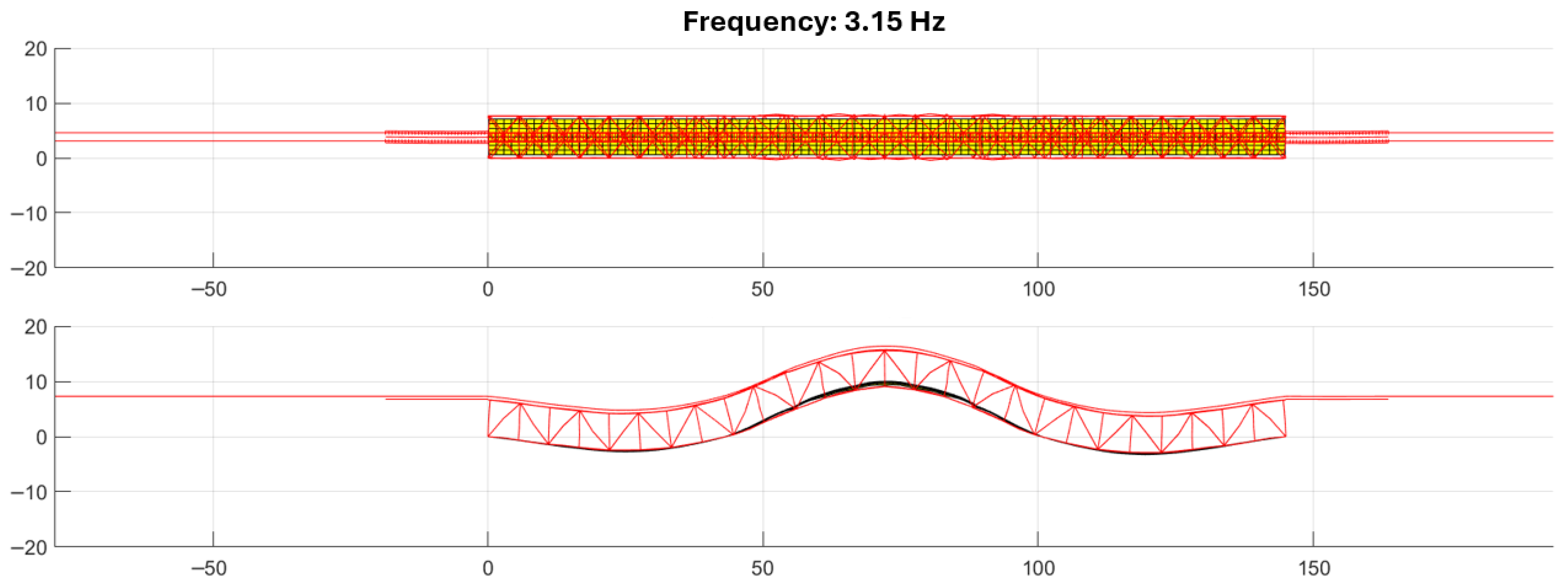
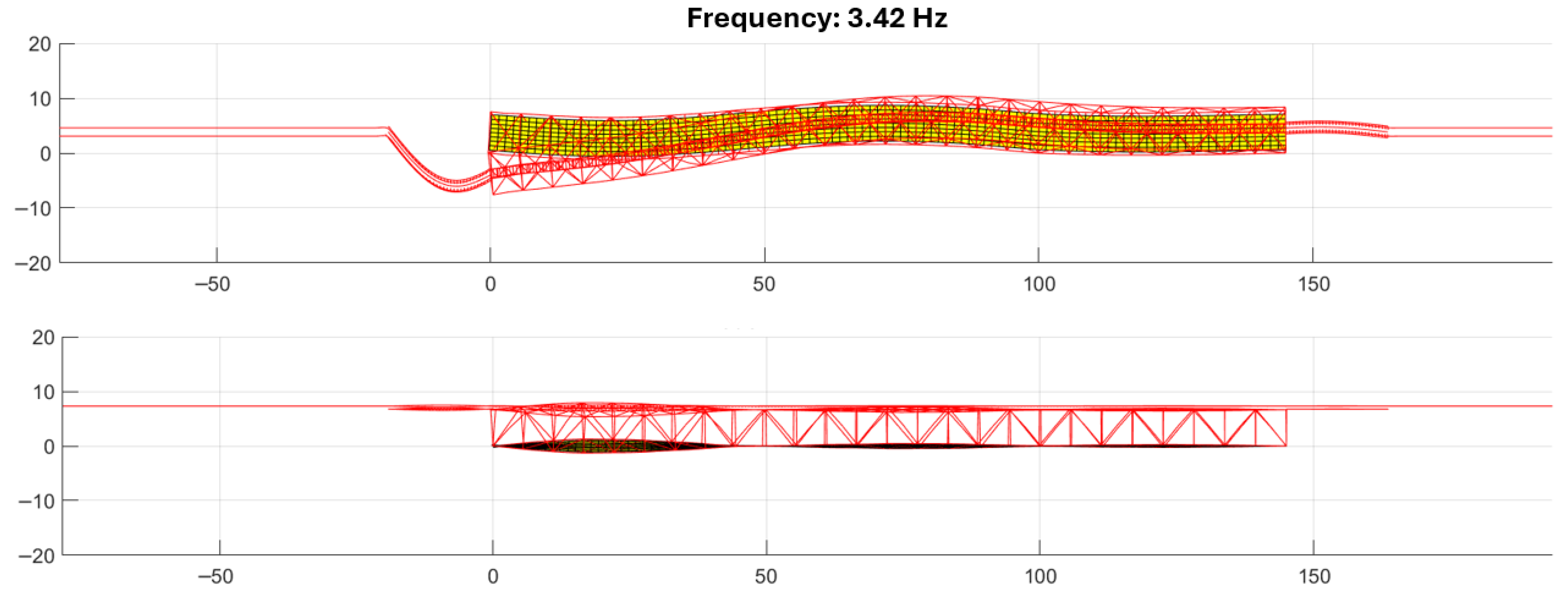
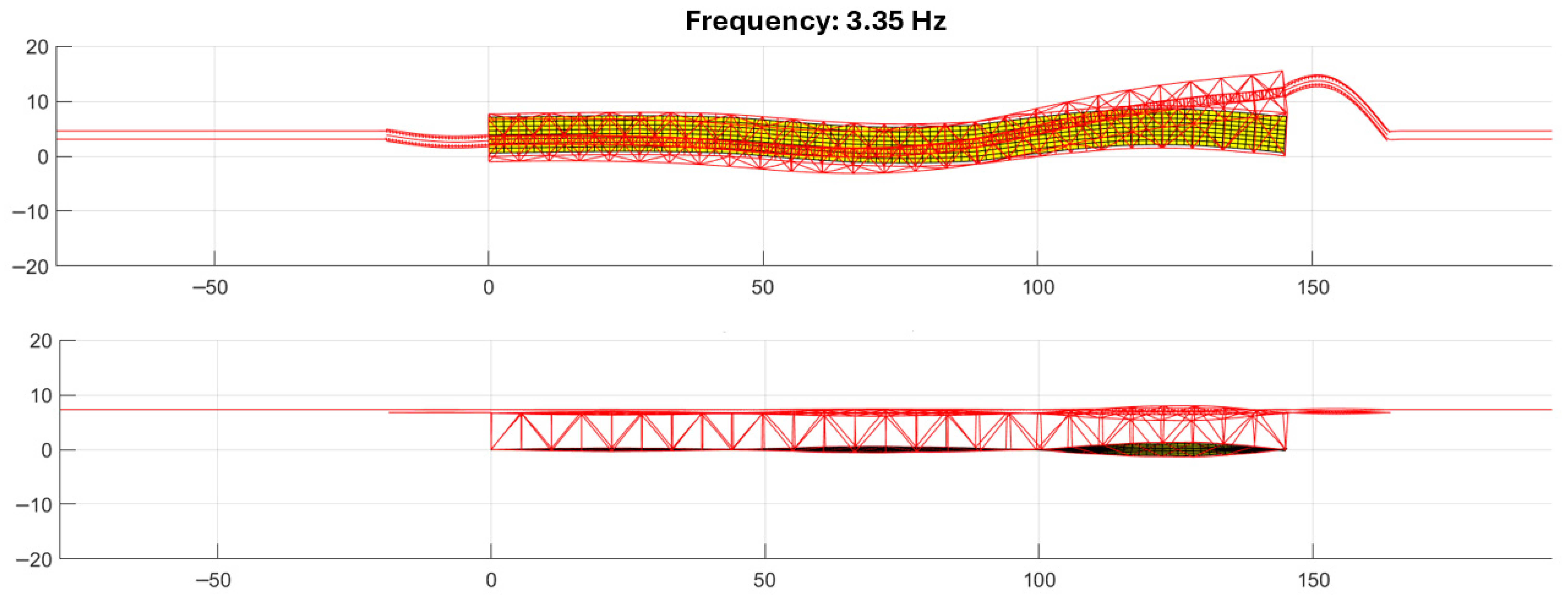
3rd Vertical	4.66	4.50	3.43	0.98

, compared with experimental counterparts computed during the preliminary campaign. By computing the MAC between numerical and experimental mode shapes, it is possible to notice that vertical mode shapes are better represented by the calibrated model compared to the lateral ones. However, the frequencies associated with the two lateral modes present differences below the 2% with respect to experimental outcomes.

The train–bridge interaction simulations were carried out by considering multiple train speeds and loading configurations to investigate how changes in the passing vehicle affect the structural response and test the robustness of the algorithm. The adopted vehicle is representative of a regional commuter train, daily transiting over the monitored bridge. It consists of four coaches, each supported by two bogies; in turn, each bogie comprises two axles. Each rail coach is described by 37 degrees of freedom, and it is assumed to move at constant forward velocity. As mentioned, a set of traveling speeds was tested, from 40 to 60 km/h, with a spacing of 2 km/h. Moreover, different coach masses were considered in an attempt to represent different passengers’ occupation of the train during the daily traffic. Being this work a preliminary study to investigate the capability of the presented algorithm in capturing structural damages, track irregularity is not accounted for and measuring noises are neglected. However, a certain degree of variability in operational loading scenarios is considered in this work. Precisely, a passenger train with five different configurations in terms of car body mass is modeled, traveling on the structure with different speeds, for different runs (see Section 4.1 for details).

As briefly recalled before, train–track–bridge dynamic simulation was carried out with ADTreS software [45], which enables FE modeling of track/bridge structures and the modeling of the rail vehicle through a multi-body approach. Structure and train are represented as two different sub-systems coupled through contact-forces, exchanged at the wheel–rail interface [46]. Time integration is performed using a modified Newmark approach (to account for non-linearities in the problem), discussed by Bernardini et al. [48].

Regarding damages applied to the numerical model of the bridge under analysis, three scenarios are considered:

• Global corrosion (GC) implemented through a uniform reduction of 5% in both Young’s modulus and material density (for steel material) applied to all truss elements of the structure. The test enables the assessment of whether the anomaly indicators can detect changes that manifest coherently across all sensing locations, considering a spatially distributed mild degradation.
• Localized damage (LD) in which a localized damage in the proximity of sensor 8 (see Figure 2) is implemented through reductions of 10% in elastic modulus and density in a lateral joint of the central span. In the remaining part of the paper, this scenario is referred to as LD10.
• Another LD case (i.e., LD70) in which a localized damage in the proximity of sensor 8 is implemented through reductions of 70% in elastic modulus and density.

The elements involved in the LD10 and LD70 damage cases are pictured in Figure 3b.

The objective of the first scenario is to assess whether the anomaly indicators can detect changes that manifest coherently across all sensing locations, considering a spatially distributed mild degradation. Instead, the third and fourth scenarios emulate progressively severe local defects, allowing for evaluating whether the reconstruction error produced by the LSTM AE increases specifically in correspondence with the affected sensors while remaining consistent with healthy behavior elsewhere. Particularly, the LD70 case, introduces a significant stiffness reduction and is expected to induce more evident distortions in the vibration patterns captured by the affected channels (i.e., accelerations evaluated at the node close to the localized damage).

4. General Framework of the LSTM AE-Based Monitoring Technique

The proposed monitoring framework processes the twenty-two vertical acceleration signals collected along the bridge at a sampling frequency of $f_s=500 \mathrm{Hz}$. The continuous data stream acquired from the sensing system is segmented into fixed-length time windows of 10 s, corresponding to $N_W=5000$ samples per sensor. The multichannel acceleration signal is defined as:

$$\mathit{A}\left(t\right)=\left[a_{z,1}\right(t) a_{z,2}(t) \dots a_{z,22}(t\left)\right]$$

(1)

with $\mathbf{A}\left(t\right)\in {\mathbb{R}}^{1\times 22}$. The signal is partitioned using a sliding-window scheme with partial overlap. By denoting with $L$ the window length and $S$ the step size ($S<L$), the $i$-th window ${\mathbf{X}}_i$ is defined as:

$${\mathbf{W}}_i=\left[\begin{array}{c}\mathbf{A}\left(t_i\right)\\ \mathbf{A}\left(t_i+1\right)\\ ⋮\\ \mathbf{A}\left(t_i+L-1\right)\end{array}\right]\in {\mathbb{R}}^{L\times 22}$$

(2)

where the window start index is given by:

$$t_i=1+(i-1)S$$

(3)

where the subscript $i=1,\dots ,n_W$ denotes the index of the sliding window in the segmentation sequence.

In the present configuration, $L=5000$ samples and $S=4000$ samples, yielding a two-second overlap between consecutive windows. Therefore, the full ten-second segment of all twenty-two acceleration channels is contained in each window ${\mathbf{X}}_i$.

The LSTM AE is independently fed by each multichannel window ${\mathbf{X}}_i$ for encoding the temporal dynamics of the multivariate signal and reconstructing a corresponding output window ${\widehat{\mathbf{X}}}_i$.

The deviation between the measured and reconstructed vertical accelerations is quantified through the reconstruction error matrix:

$${\mathbf{E}}_i={\mathbf{X}}_i-{\widehat{\mathbf{X}}}_i$$

(4)

The per-sensor Root Mean Square Error (RMSE) is computed as:

$${\mathrm{R}\mathrm{M}\mathrm{S}\mathrm{E}}_{i,j}=\sqrt{{\displaystyle \frac{1}{L}}\sum _{k=1}^L\left(X_i\right(k,j)-{\widehat{X}}_i(k,j){)}^2},j=1,\dots ,22$$

(5)

Therefore, for each time window, a feature vector ${\mathrm{R}\mathrm{M}\mathrm{S}\mathrm{E}}_i\in {\mathbb{R}}^{1\times 22}$ that characterizes the reconstruction quality of the full sensor array is obtained.

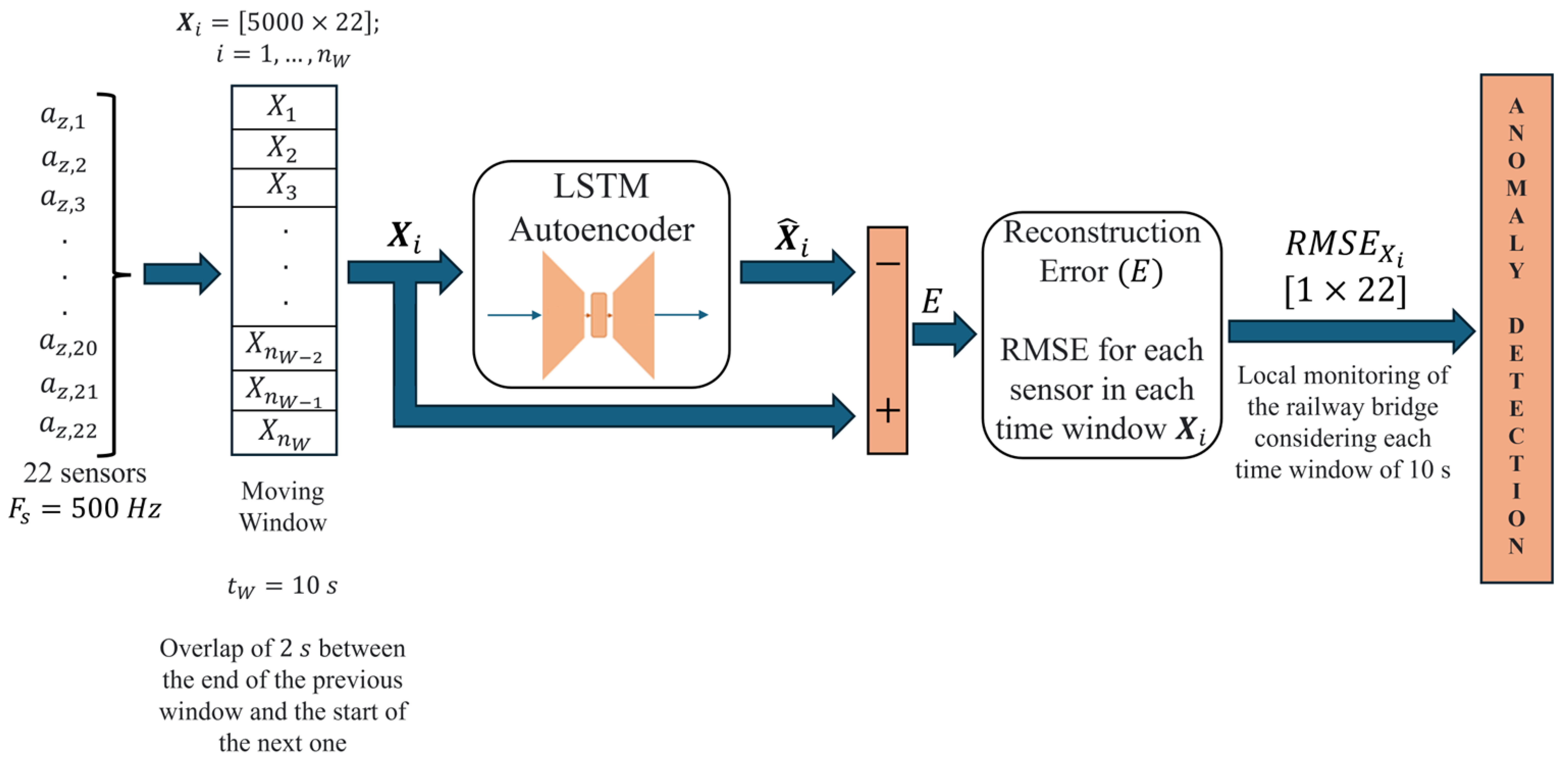
The RMSE values are subsequently compared against sensor-level (local) and global thresholds, learned from healthy-condition data during the training stage of the LSTM AE, to determine whether window ${\mathbf{X}}_i$ and its associated sensors are consistent with nominal structural behavior or indicative of a potential anomaly. The entire procedure is summarized schematically in Figure 4. The proposed approach introduces specific design choices tailored to multichannel structural monitoring of railway bridges, extending standard reconstruction-based anomaly detection approaches. Multichannel vibration data are exploited to jointly capture temporal and spatial dependencies of the structural response, rather than analyzing each sensor independently. Furthermore, anomaly detection is carried out by introducing a dual-threshold strategy, combining a global window-level criterion with sensor-specific thresholds, enabling the identification of both distributed and localized anomalies. Finally, the methodology adopts a fully unsupervised training strategy based exclusively on healthy-condition datasets, making it suitable for SHM applications where labeled damage data are not available.

The proposed neural network architecture is designed as a sequence-to-sequence LSTM AE [49,50] specifically developed for the reconstruction of multichannel vibration signals associated with the dynamic behavior of the monitored railway bridge. The neural network model operates on time series composed of twenty-two simultaneous acceleration channels, exploiting both the temporal dependencies and the spatial correlations inherent in the structural response. By learning a compact latent representation of the normal-state dynamics and by enforcing accurate sequence reconstruction, the LSTM AE provides a reliable, fully data-driven basis for identifying deviations indicative of structural anomalies. The LSTM AE is composed of three main components: the encoder, the bottleneck, and the decoder, represented by three LSTM layers, respectively. For a more detailed description of the architecture of the LSTM AE, please refer to Appendix B.1.

4.1. Training Dataset Generation

The training dataset used to calibrate the LSTM AE is constructed exclusively from the healthy structural conditions of the monitored railway bridge. To this end, a comprehensive numerical campaign is performed by simulating the coupled train–bridge dynamic interaction using the modeling framework described in Section 2. Five railway vehicle configurations, denoted as Train-A, Train-B, Train-C, Train-D and Train-E, are considered. Specifically, each railway vehicle consists of four car bodies, each car body is mounted on two bogies, and each bogie is equipped with two wheelsets. The properties of the five configurations differ only in the mass of the four car bodies, as reported in

Table 2. The main characteristics of the considered railway vehicles. Variability is introduced in the car body mass to simulate different passenger occupations among different runs. Please notice that stiffness and damping values for primary and secondary suspensions refer to each single bogie.

	Train-A	Train-B	Train-C	Train-D	Train-E
Car body 1 mass [kg]	48,020	46,372	49,310	49,307	44,470
Car body 2 mass [kg]	45,852	38,996	46,353	42,286	45,936
Car body 3 mass [kg]	39,246	40,531	39,506	44,960	44,890
Car body 4 mass [kg]	48,911	45,600	49,428	41,940	49,330
Bogie 1 mass [kg]	3318	3318	3318	3318	3318
Bogie 2 mass [kg]	6100	6100	6100	6100	6100
Wheelset 1 mass [kg]	1916	1916	1916	1916	1916
Wheelset 2 mass [kg]	1926	1926	1926	1926	1926
Prim. vert. stiff. 1 [kN/m]	3832	3832	3832	3832	3832
Prim. vert. damp. 1 [kNs/m]	40	40	40	40	40
Prim. vert. stiff. 2 [kN/m]	5200	5200	5200	5200	5200
Prim. vert. damp. 2 [kNs/m]	64	64	64	64	64
Sec. vert. stiff. 1 [kN/m]	770	770	770	770	770
Sec. vert. damp. 1 [kNs/m]	72	72	72	72	72
Sec. vert. stiff. 2 [kN/m]	830	830	830	830	830
Sec. vert. damp. 2 [kNs/m]	72	72	72	72	72

, introducing variability in the dynamic excitation.

The dynamic railway vehicle–bridge interaction is simulated over a range of cruising speeds from 40 km/h to 60 km/h, with increments of 2 km/h, for each railway vehicle. The vertical acceleration response of the bridge is recorded during each simulated railway vehicle passage, at the twenty-two positions corresponding to the ones related to the virtually mounted sensors on the bridge model, sampled at $f_s=500 \mathrm{Hz}.$ By considering a railway vehicle configuration $T\in \{\mathrm{Train}\text{-}\mathrm{A},\mathrm{Train}\text{-}\mathrm{B},\mathrm{Train}\text{-}\mathrm{C},\mathrm{Train}\text{-}\mathrm{D},\mathrm{Train}\text{-}\mathrm{E}\}$, the resulting multi-sensor signal is denoted as:

$${\mathit{X}}_{\mathrm{healthy},\mathit{T}}={\mathit{a}}_{\mathit{z},\mathit{T}}\in {\mathbb{R}}^{L_T\times 22}$$

(6)

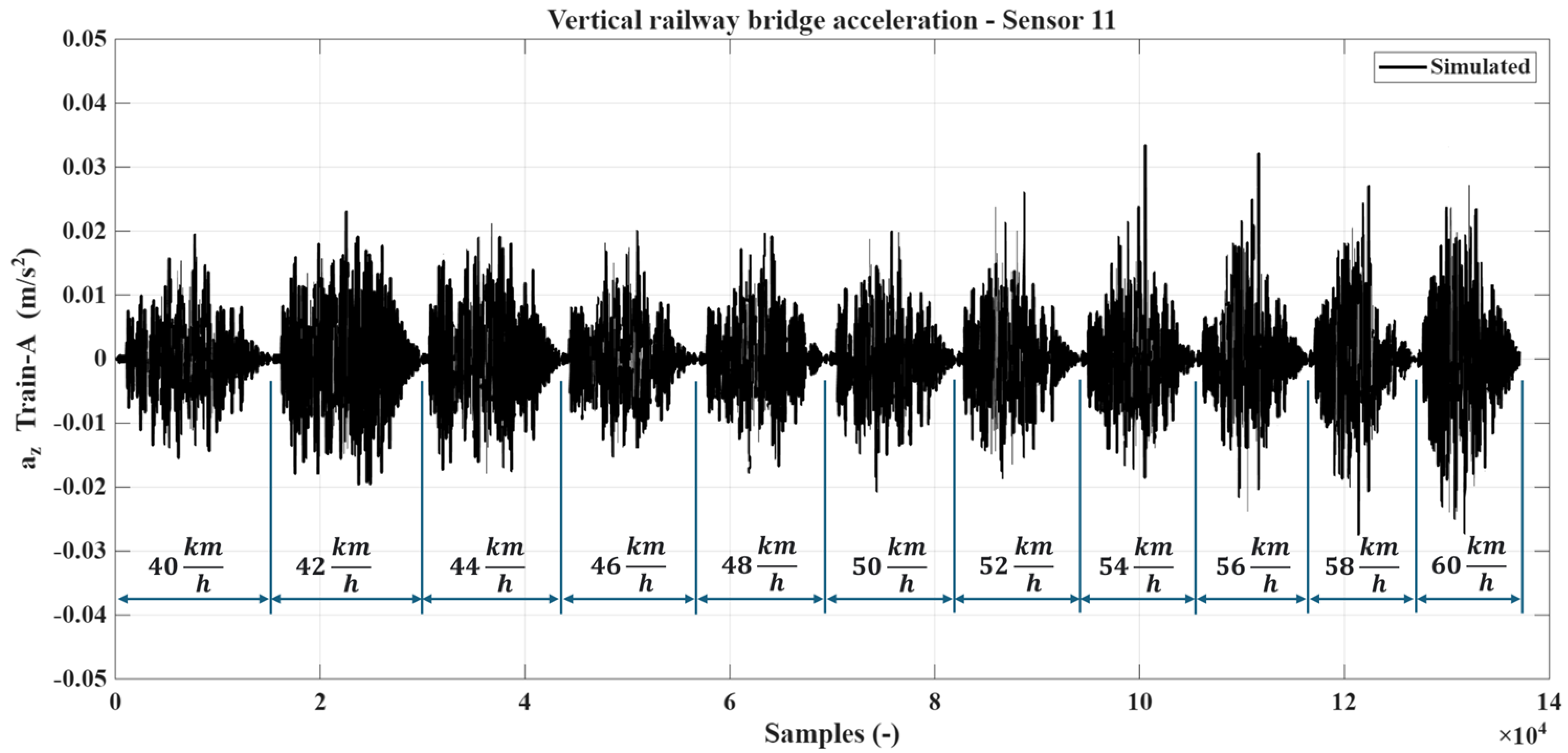
where $L_T$ is the total number of samples obtained by concatenating the acceleration histories corresponding to all simulated speeds. An example of the resulting multi-speed time series for Sensor 11 considering Train-A is shown in Figure 5, illustrating the succession of vibration signatures generated by the speed-incremented passages.

The fixed-size input sequences for the LSTM AE are obtained by segmenting each multichannel signal $X_{\mathrm{healthy},T}$ into partially overlapping windows of 10 s duration. For each train configuration $T$, the $i$-th window is defined as:

$$W_{\mathrm{healthy},T,i}=\left[\begin{array}{c}{X}_{\mathrm{healthy},T}\left(t_i,22\right)\\ X_{\mathrm{healthy},T}\left(t_i+1,22\right)\\ ⋮\\ X_{\mathrm{healthy},T}\left(t_i+L-1,22\right)\end{array}\right]\in {\mathbb{R}}^{L\times 22}$$

(7)

where the window-start index is:

$$t_i=1+\left(i-1\right)S, i=\mathrm{1,2},\dots ,N_T$$

(8)

where $L=5000$ and $S=4000$ denote the number of samples per window (10 s at 500 Hz) and the step size between consecutive windows, respectively, corresponding to an overlap of 2 s, and $N_T$ denotes the number of 10 s segments, which corresponds to 34 time windows per train. The previously described window length was adopted as a compromise between temporal resolution and the need to preserve a sufficiently rich description of the bridge’s vibration response during train passages. The LSTM AE is enabled to capture multiple cycles of the dominant bending and torsional modes, as well as the spatially evolving excitation produced by successive axle crossings. Shorter windows would have reduced the amount of dynamic information available to the network, limiting its ability to learn medium- and long-range temporal dependencies and to represent non-stationary effects induced by the moving load. Longer time windows have not been chosen due to the higher computational and memory requirements of the sequence-to-sequence training procedure without providing commensurate benefits in terms of anomaly detectability. The adopted duration, therefore, offers a balanced trade-off between dynamic content, computational efficiency, and temporal resolution.

The total number of windows across the five train configurations is:

$$N_{\mathrm{segments}}=\sum _T{N}_T=170$$

(9)

Each of the collected $N_{\mathrm{segments}}$ represents a ten-second realization of the bridge response under healthy operating conditions. All time windows are then aggregated into a single dataset:

$$W_{\mathrm{healthy},\mathrm{TOT}}=\{W_{\mathrm{healthy},T,i} \mid T \in \{\mathrm{Train}\text{-}\mathrm{A},\mathrm{T}\mathrm{r}\mathrm{a}\mathrm{i}\mathrm{n}\text{-}\mathrm{B}, \mathrm{Train}\text{-}\mathrm{C}, \mathrm{Train}\text{-}\mathrm{D}, \mathrm{Train}\text{-}\mathrm{E}\}, i=1,\dots ,N_T\}$$

(10)

which constitutes the complete collection of healthy-condition samples. The healthy dataset is divided into two subsets to avoid data leakage. Specifically, 70% of $W_{\mathrm{healthy},\mathrm{TOT}}$ named $W_{\mathrm{healthy}}$, equalling 119 time windows, is employed for training the LSTM AE. The remaining 30% of $W_{\mathrm{healthy},\mathrm{TOT}}$, equal to 51 time windows, is used for testing the proposed LSTM AE. Furthermore, the testing healthy dataset is employed to define both the global and sensor-specific anomaly detection thresholds, described in the following Sections, based on the reconstruction error. A standardization process, based on the Z-score rule, is made on each time window before feeding it to the LSTM AE. For each sensor channel $j$, the normalized sample is computed as:

$$W_{\mathrm{healthy},\mathrm{std}}\left(k,j\right)={\displaystyle \frac{W_{\mathrm{healthy}}\left(k,j\right)-{\mu }_{healthy,j}}{{\sigma }_{healthy,j}}}, k=1,\dots , 5000$$

(11)

where ${\mu }_{healthy,j}$ and ${\sigma }_{healthy,j}$ denote the sample mean and standard deviation of channel $j=1,\dots ,22$, respectively, computed across the entire healthy dataset. Furthermore, the standardization parameters used in the Z-score consist of two vectors ${\mathit{\mu }}_{\mathit{h}\mathit{e}\mathit{a}\mathit{l}\mathit{t}\mathit{h}\mathit{y}}, {\mathit{\sigma }}_{\mathit{h}\mathit{e}\mathit{a}\mathit{l}\mathit{t}\mathit{h}\mathit{y}}\in {\mathbb{R}}^{1\times 22}$ each containing the sample mean and standard deviation computed independently for each of the twenty-two sensor channels, respectively. This channel-wise standardization ensures a consistent scaling of the input features, preserving the relative dynamic variability across the sensing array, which is essential for the stable training of the LSTM AE.

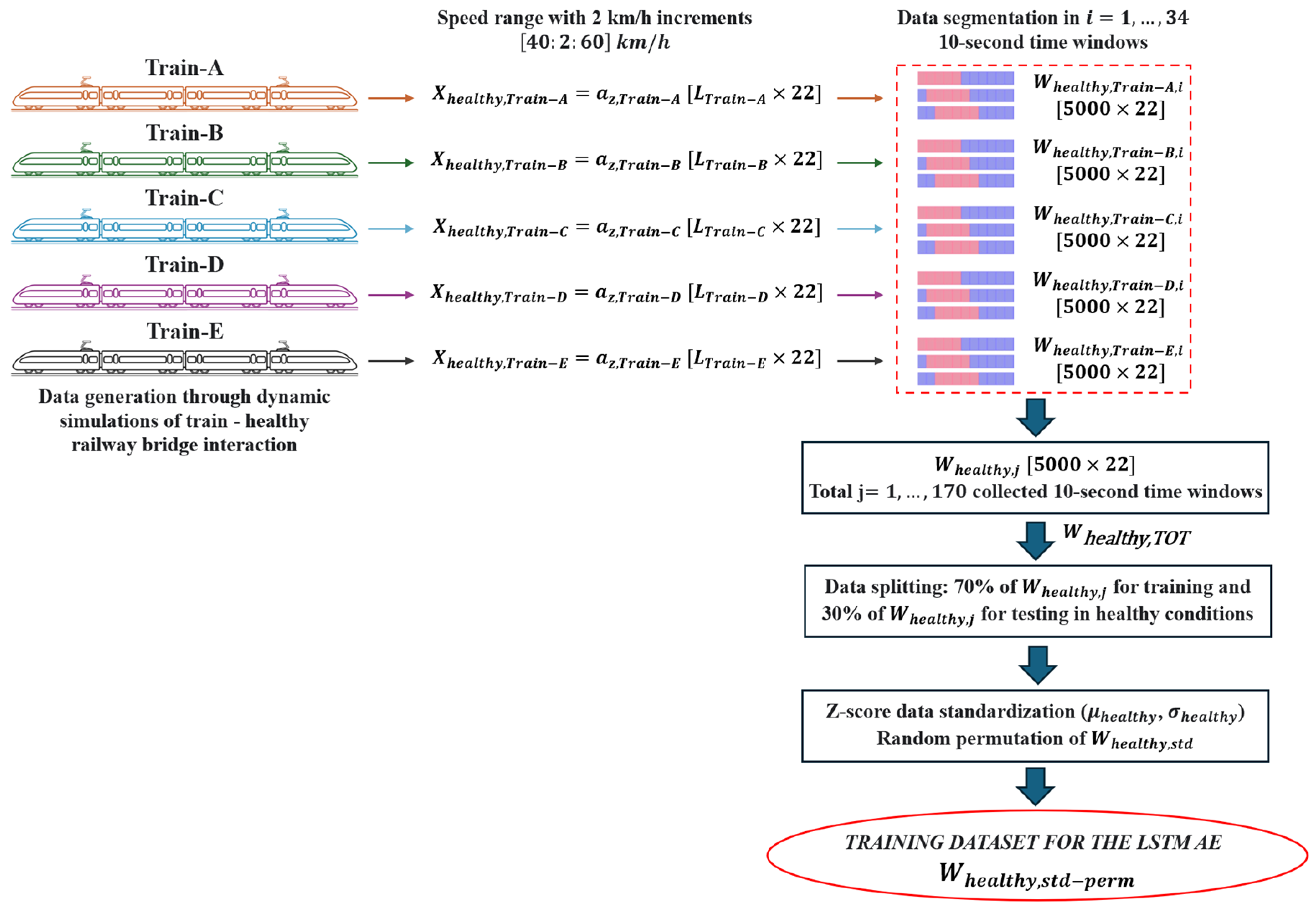
The LSTM AE presented in Section 4, and detailed in Appendix B.1, is trained employing the final training dataset $W_{\mathrm{healthy},\mathrm{std}\text{-}\mathrm{perm}}$, which is constituted of randomly permuted standardized time windows. The random permutation removes any residual ordering effects associated with railway vehicle type or speed. A schematic representation of the dataset-generation workflow is provided in Figure 6.

4.2. LSTM AE Training and Optimization

The LSTM AE training process is integrated into a Bayesian Optimization (BO) framework for identifying the configuration of hyperparameters that minimizes the reconstruction error. Furthermore, the coupling between the BO and the LSTM AE training ensures stable convergence and adequate regularization under the heterogeneous excitation scenarios considered in the healthy-condition dataset.

Details on the theory behind Bayesian Optimization and how it was performed are included in Appendix B.2.

The optimization converges towards a configuration that achieves a favorable trade-off between network expressiveness, generalization ability, and training stability.

The selected configuration features include an encoder of 116 units, a bottleneck layer of 58 units defined as half of the encoder size, and a decoder symmetric to the encoder.

The values of optimized dropout probabilities associated with the encoder and bottleneck outputs are 0.15545 and 0.20608, respectively, indicating that moderate stochastic regularization was instrumental in preventing co-adaptation of recurrent features. The initial learning rate converges to $0.0018109$, ensuring both sufficiently rapid initial descent and stable refinement of the weights near convergence. The optimized ${\mathcal{l}}_2$-regularization coefficient assumes the value $1.1654\times {10}^{-6}$, effectively limiting weight growth without suppressing the capability of the LSTM AE to represent the intrinsic variability of healthy-condition vibrations. An optimal mini-batch size of 16 samples is selected, reflecting the gradient sensitivity to temporal fluctuations in multichannel sequences. A summary of the optimized hyperparameters and the associated training performance is reported in

Table 3. Optimized hyperparameters and resulting training performance.

Hyperparameter	Value
Encoder units	$116$
Bottleneck units	$58$
Decoder units	$116$
Dropout 1	$0.15545$
Dropout 2	$0.20608$
Initial learning rate	$0.0018109$
${\mathcal{l}}_2$-regularization	$1.1654\times {10}^{-6}$
Mini-batch size	$16$
Final RMSE (Bayesian Optimization)	$0.046981$
Final training MSE	$0.014$
Epochs	$100$

.

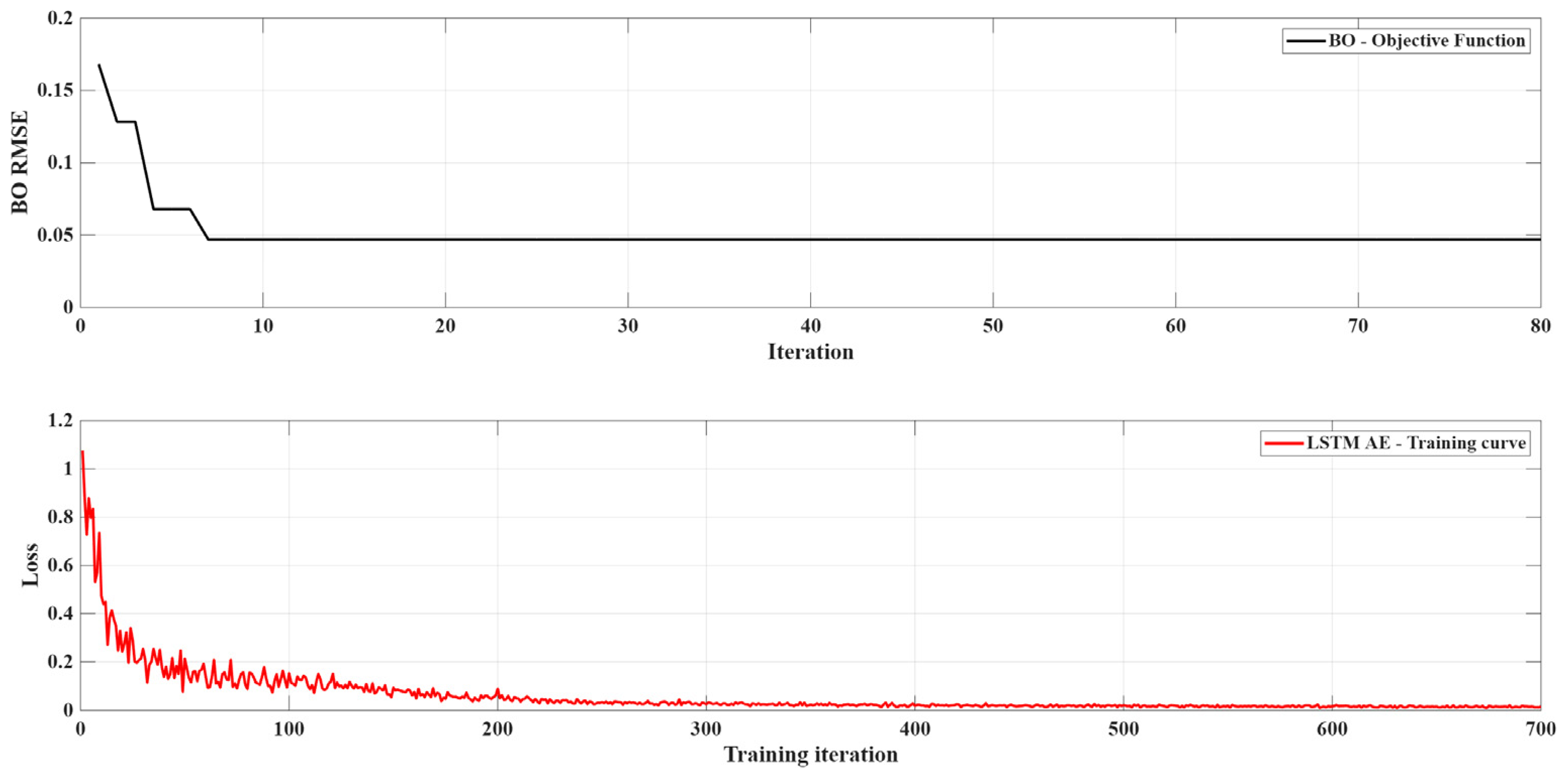
A quick decrease in the RMSE is observable in Figure 7 during the initial iterations of the BO. The surrogate model progressively identifies hyperparameter regions associated with improved reconstruction performance. A plateau is reached by the BO procedure around the tenth iteration, indicating that the search space contains a relatively narrow region of high-performing configurations. The early stabilization of the RMSE also confirms the adequacy of the selected hyperparameter ranges, which are sufficiently broad to encompass the optimal configuration yet restrictive enough to avoid pathological regimes that could lead to unstable training dynamics.

Furthermore, Figure 7 shows the training curve of the optimal LSTM AE, which exhibits a monotonic decay of the loss function, confirming that the network learns to reproduce the healthy-condition vibration patterns. Specifically, a sharp decrease in the loss function can be observed in the first 100–150 iterations, reflecting the rapid adjustment of the recurrent and fully connected layers in capturing the dominant components of the input sequences.

A steady refinement phase over several hundred iterations follows the initial transient, in which the network progressively stabilizes its internal representation and reduces residual reconstruction errors.

The absence of oscillations, divergences, or sudden loss spikes confirms the numerical stability of the optimized hyperparameters and demonstrates the effectiveness of the adopted regularization strategy, particularly the moderate dropout rates and ${\mathcal{l}}_2$-penalty, in preventing overfitting.

The complete training process, integrated with the Bayesian Optimization one, required approximately one day on a workstation equipped with an NVIDIA GeForce RTX 3090 GPU. Although the number of independent simulations is limited, the dataset comprises many multichannel time windows obtained through signal segmentation. A sufficiently rich representation of the structural response under different operating conditions is provided by the used windows, including variations in train speed and loading configurations. Furthermore, the proposed approach is fully unsupervised, aiming to learn the nominal structural behavior in healthy conditions rather than performing classification tasks, which reduces the dependency on large, labeled datasets.

4.3. Anomaly Detection Criteria

After training the LSTM AE on healthy-condition data, anomaly detection is performable by evaluating the discrepancy between the measured multichannel acceleration windows and their reconstructed counterparts. Since the training dataset was standardized using the channel-wise mean and standard deviation vectors ${\mathit{\mu }}_{\mathit{h}\mathit{e}\mathit{a}\mathit{l}\mathit{t}\mathit{h}\mathit{y}}, {\mathit{\sigma }}_{\mathit{h}\mathit{e}\mathit{a}\mathit{l}\mathit{t}\mathit{h}\mathit{y}}\in {\mathbb{R}}^{1\times 22}$, stored during the dataset generation described in Section 4.1, all reconstructed windows are first de-standardized using these parameters before computing the detection metrics, ensuring that reconstruction errors are assessed in physically meaningful units consistent across both training and testing phases.

For a given window $W_i\in {\mathbb{R}}^{L\times 22}$ and sensor channel $j$, the reconstruction error is quantified by the Root Mean Square Error (RMSE):

$${\mathrm{R}\mathrm{M}\mathrm{S}\mathrm{E}}_{i,j}=\sqrt{{\displaystyle \frac{1}{L}}\sum _{k=1}^L{\left(W_i\right(k,j)-{\widehat{W}}_i(k,j\left)\right)}^2}$$

(12)

where $L=5000$ is the window length in samples. The set of per-sensor reconstruction errors for window $i$ forms the vector:

$${\mathrm{R}\mathrm{M}\mathrm{S}\mathrm{E}}_i=[{\mathrm{R}\mathrm{M}\mathrm{S}\mathrm{E}}_{i,1},\dots ,{\mathrm{R}\mathrm{M}\mathrm{S}\mathrm{E}}_{i,22}]\in {\mathbb{R}}^{1\times 22}$$

(13)

A global anomaly indicator for each window is defined as the Euclidean norm of this vector:

$$E_i={\parallel {\mathrm{R}\mathrm{M}\mathrm{S}\mathrm{E}}_i\parallel }_2=\sqrt{\sum _{j=1}^{22}{\mathrm{R}\mathrm{M}\mathrm{S}\mathrm{E}}_{i,j}^2}$$

(14)

Statistic-based thresholds for anomaly detection [51,52] are computed exclusively from healthy-condition training windows, and once calculated, they are stored for use in operational monitoring. For each sensor $j$, the threshold, based on the three-sigma statistical rule, is defined as:

$${\mathrm{t}\mathrm{h}\mathrm{r}}_j={\mu }_j^{\left(\mathrm{R}\mathrm{M}\mathrm{S}\mathrm{E}\right)}+3{\sigma }_j^{\left(\mathrm{R}\mathrm{M}\mathrm{S}\mathrm{E}\right)}$$

(15)

where ${\mu }_j^{\left(\mathrm{R}\mathrm{M}\mathrm{S}\mathrm{E}\right)}$ and ${\sigma }_j^{\left(\mathrm{R}\mathrm{M}\mathrm{S}\mathrm{E}\right)}$ are the mean and standard deviation of ${\mathrm{R}\mathrm{M}\mathrm{S}\mathrm{E}}_{i,j}$ computed across all healthy training windows. Analogously, the global threshold associated with the indicator $E_i$ is given by:

$${\mathrm{t}\mathrm{h}\mathrm{r}}_E={\mu }_E+3 {\sigma }_E, {\mu }_E=\mathrm{m}\mathrm{e}\mathrm{a}\mathrm{n}\left(E_i\right), {\sigma }_E=\mathrm{s}\mathrm{t}\mathrm{d}\left(E_i\right)$$

(16)

A window is flagged as anomalous whenever either the sensor-level error or the global indicator exceeds the corresponding healthy threshold. The three-sigma rule, based on the empirical distribution of the reconstruction errors, has been chosen to provide a simple and interpretable statistical criterion for identifying deviations from nominal behavior observed under healthy conditions linked to the testing dataset described in Section 4.1. Furthermore, the 3$\sigma$-based threshold has been selected, after a sensitivity analysis, as a compromise between the 2$\sigma$- and 4$\sigma$-based thresholds. Particularly, the lower threshold 2$\sigma$ led to excessive sensitivity, resulting in false positives in both healthy and faulty conditions. In contrast, the higher threshold 4$\sigma$ reduced the sensitivity of the proposed method, limiting its capability to detect damage scenarios. Therefore, the 3$\sigma$-based threshold represents a trade-off between reliability and sensitivity, minimizing false alarms during anomaly detection.

For sensor $j$, the Positive Rate (PR) is therefore computed as:

$${\mathrm{P}\mathrm{R}}_j={\displaystyle \frac{1}{N_{\mathrm{w}\mathrm{i}\mathrm{n}}}}\sum _{i=1}^{N_{\mathrm{w}\mathrm{i}\mathrm{n}}}\mathbb{I}({\mathrm{R}\mathrm{M}\mathrm{S}\mathrm{E}}_{i,j}>{\mathrm{t}\mathrm{h}\mathrm{r}}_j)$$

(17)

where $N_{\mathrm{w}\mathrm{i}\mathrm{n}}$ is the number of evaluated windows and $\mathbb{I}(\cdot )$ is the indicator function:

$$\mathbb{I}\left(A\right)=\left\{\begin{array}{c}1, if the event A is true\\ 0, if the event A is false\end{array}\right.$$

(18)

The corresponding complement is defined as the Reliability Index (RI) of the j-th sensor:

$${\mathrm{R}\mathrm{I}}_j=1-{\mathrm{P}\mathrm{R}}_j$$

(19)

Similarly, the global Positive Rate based on the composite indicator $E_i$ is:

$${\mathrm{P}\mathrm{R}}_{\mathrm{g}\mathrm{l}\mathrm{o}\mathrm{b}}={\displaystyle \frac{1}{N_{\mathrm{w}\mathrm{i}\mathrm{n}}}}\sum _{i=1}^{N_{\mathrm{w}\mathrm{i}\mathrm{n}}}\mathbb{I}(E_i>{\mathrm{t}\mathrm{h}\mathrm{r}}_E)$$

(20)

with global RI:

$${\mathrm{R}\mathrm{I}}_{\mathrm{g}\mathrm{l}\mathrm{o}\mathrm{b}}=1-{\mathrm{P}\mathrm{R}}_{\mathrm{g}\mathrm{l}\mathrm{o}\mathrm{b}}$$

(21)

The reliability of the detection process has been enhanced by introducing a stricter two-window consistency rule. Under this criterion, an anomaly is declared only if two consecutive windows exceed the same threshold. For sensor $j$, this corresponds to:

$$\mathbb{I}({\mathrm{R}\mathrm{M}\mathrm{S}\mathrm{E}}_{i,j}>{\mathrm{t}\mathrm{h}\mathrm{r}}_j) \wedge \mathbb{I}({\mathrm{R}\mathrm{M}\mathrm{S}\mathrm{E}}_{i+1,j}>{\mathrm{t}\mathrm{h}\mathrm{r}}_j)$$

(22)

where $\wedge$ denotes the logical AND operator. The associated positive rate is therefore:

$${\mathrm{P}\mathrm{R}}_j^{\left(2\mathrm{w}\mathrm{i}\mathrm{n}\right)}={\displaystyle \frac{1}{N_{\mathrm{w}\mathrm{i}\mathrm{n}}}}\sum _{i=1}^{N_{\mathrm{w}\mathrm{i}\mathrm{n}}}\mathbb{I}({\mathrm{R}\mathrm{M}\mathrm{S}\mathrm{E}}_{i,j}>{\mathrm{t}\mathrm{h}\mathrm{r}}_j \wedge {\mathrm{R}\mathrm{M}\mathrm{S}\mathrm{E}}_{i+1,j}>{\mathrm{t}\mathrm{h}\mathrm{r}}_j)$$

(23)

with RI:

$${\mathrm{R}\mathrm{I}}_j^{\left(2\mathrm{w}\mathrm{i}\mathrm{n}\right)}=1-{\mathrm{P}\mathrm{R}}_j^{\left(2\mathrm{w}\mathrm{i}\mathrm{n}\right)}$$

(24)

An analogous formulation applies to the global indicator $E_i$ under the same consistency rule. The complete anomaly detection framework, which includes both the single-window and the two-window criteria, establishes a set of decision rules that can later be applied to identify deviations from the healthy structural behavior, including potential cases where consecutive windows exhibit consistent increases in reconstruction error. Additionally, the Precision, Recall, and the F1-score are computed to highlight the detection performance across the considered scenarios. Specifically, by considering the following ground-truth:

$$y_{truth,j}=\left\{\begin{array}{c}1, if damaged\\ 0, if healthy\end{array}\right.; j=1,\dots , 22 \mathrm{s}\mathrm{e}\mathrm{n}\mathrm{s}\mathrm{o}\mathrm{r}\mathrm{s}$$

(25)

a candidate sensor $y_j(j=1,\dots , 22)$ takes the value 1, detecting damage, if and only if ${\mathrm{P}\mathrm{R}}_j>0$, otherwise $y_j$ takes the value 0, highlighting the healthy condition of the bridge around its positioning. Therefore, the true positive (TP), false positive (FP), true negative (TN), and false negative (FN) values can be computed as follows:

$$\begin{array}{c}T{P}_j=\left(y_j=1\right)\wedge \left(y_{truth,j}=1\right)\\ F{P}_j=\left(y_j=1\right)\wedge \left(y_{truth,j}=0\right)\\ T{N}_j=\left(y_j=0\right)\wedge \left(y_{truth,j}=0\right)\\ F{N}_j=\left(y_j=0\right)\wedge \left(y_{truth,j}=1\right)\end{array}$$

(26)

Finally, the Precision, Recall, and the F1-score metrics are evaluated as follows:

$$\begin{array}{c}Precisio{n}_j={\displaystyle \frac{T{P}_j}{T{P}_j+F{P}_j}}\\ {Recall}_j={\displaystyle \frac{T{P}_j}{T{P}_j+F{N}_j}}\\ F_{1j}={\displaystyle \frac{2\cdot Precisio{n}_j\cdot Recal{l}_j}{Precisio{n}_j+Recal{l}_j}}\end{array}$$

(27)

5. Results

The performance of the optimized LSTM AE in discriminating healthy and damaged structural conditions is assessed by applying the anomaly detection framework to four test scenarios. The same neural network architecture characterized by the BO-based hyperparameters is employed in all tests. The tests include both healthy and damaged conditions of the railway bridge (see Section 3), allowing to examine the sensitivity of the reconstruction-based indicators under progressively more severe structural alterations. Other than the three damage scenarios, a healthy (H) testing scenario is considered. This test is made to verify that the LSTM AE does not produce spurious detections when exposed to new realizations of the same healthy structural behavior, and to establish a reference level of reconstruction error against which damaged conditions can be meaningfully compared. For all the tests, the window length is 10 s, as described in Section 4.1. The selected time length represents a compromise between temporal resolution and the need to capture a sufficiently rich description of the bridge dynamic response during train passages. Specifically, the chosen duration allows for the inclusion of multiple cycles of the dominant bending and torsional modes, as well as the full transient response induced by the train–bridge interaction. Shorter windows may not fully capture the relevant dynamic behavior; longer windows would reduce temporal resolution without providing significant additional information.

Across the four scenarios considered in this paper, the results presented in the following include:

• The global reconstruction error $E_i$ across time windows, together with the global anomaly threshold derived from healthy-condition training data, enabling the identification of windows whose overall dynamic response deviates from the healthy signature;
• The reconstruction error is compared between healthy and damaged scenarios by averaging, for each sensor, the RMSE over all the available time windows. This representation provides insight into which sensors are most sensitive to the imposed damage and how the anomaly manifests spatially along the structure;
• The anomaly detection performance is quantified through sensor-wise RI, computed according to the statistical thresholds established in the training step. The resulting RI curves summarize, for each sensing point, the reliability with which structural deviations are detected across all windows, through a direct performance metric. Moreover, to enhance the interpretability of the results, the sensors are grouped according to their position along the upstream and downstream sides of the railway bridge, corresponding to odd-indexed and even-indexed sensors, respectively, as shown in Figure 2.

The results presented in this study have been obtained using simulated data derived from a calibrated finite element model of the railway bridge. This allowed for a controlled and physically consistent evaluation of the proposed methodology. In contrast, real-world factors such as measurement noise, track irregularities, and environmental variability are not considered, introducing a domain gap between simulated and real monitoring conditions. However, the proposed framework is based on learning the intrinsic behavior of the structure under healthy conditions through multichannel time-series data, which is expected to mitigate the impact of noise and variability typically observed in real monitoring scenarios. The methodology will be validated using experimental data acquired from the monitored bridge in future research. For the tests that consider the railway bridge in damaged conditions, the physical sequence of time windows adopted as input for the trained LSTM AE follows that presented in Figure 5.

5.1. Healthy Test

The internal consistency of the proposed anomaly detection framework is verified through the present test by applying the LSTM AE to vibration data corresponding to healthy structural conditions only. The time windows, belonging to the testing dataset described in Section 4, are randomly ordered. The capability of the network to correctly recognize healthy conditions without generating spurious alarms, and the definition of per-sensor and global thresholds from undamaged structural behavior, constitute the assessments of the present analysis.

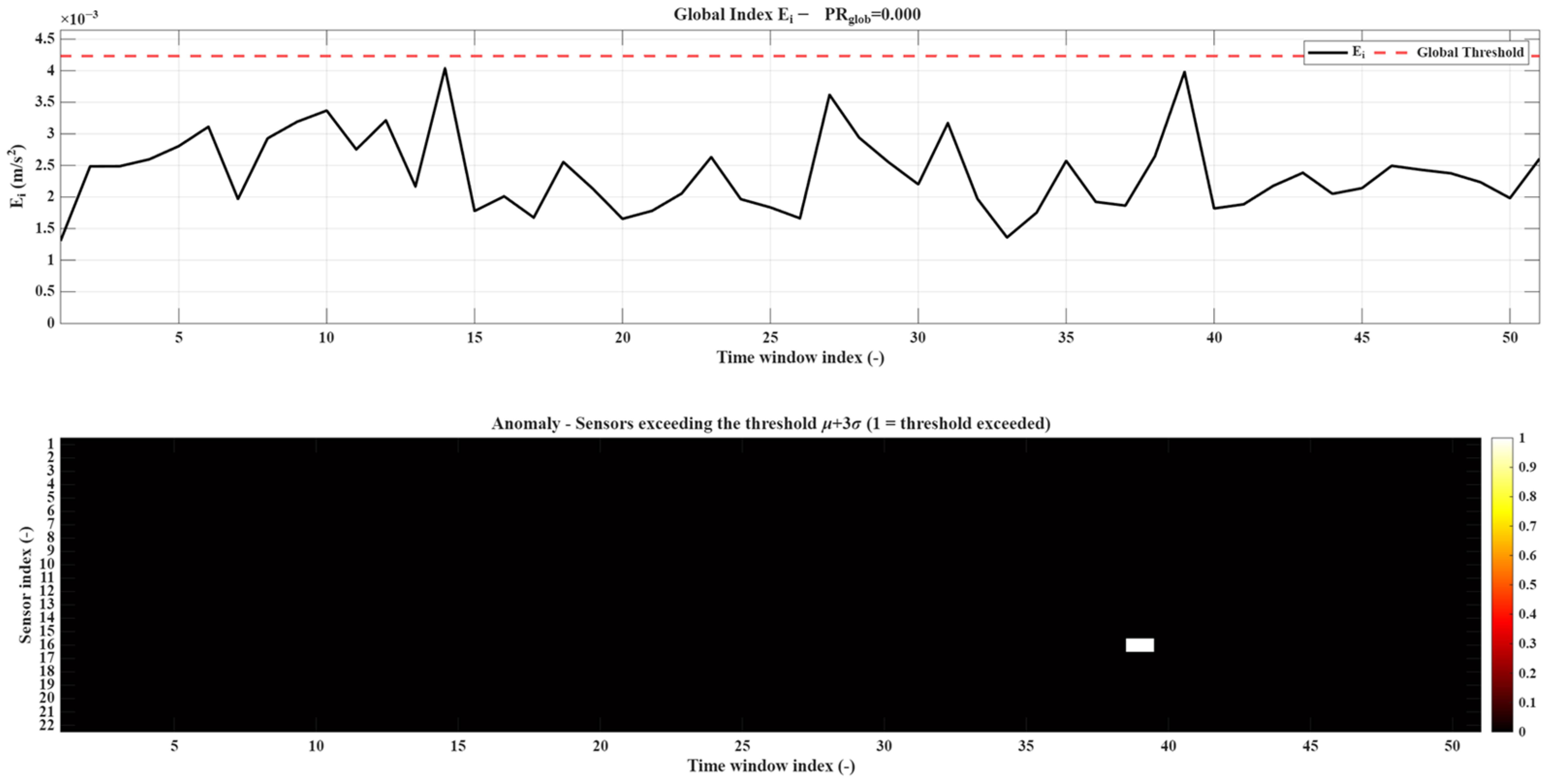
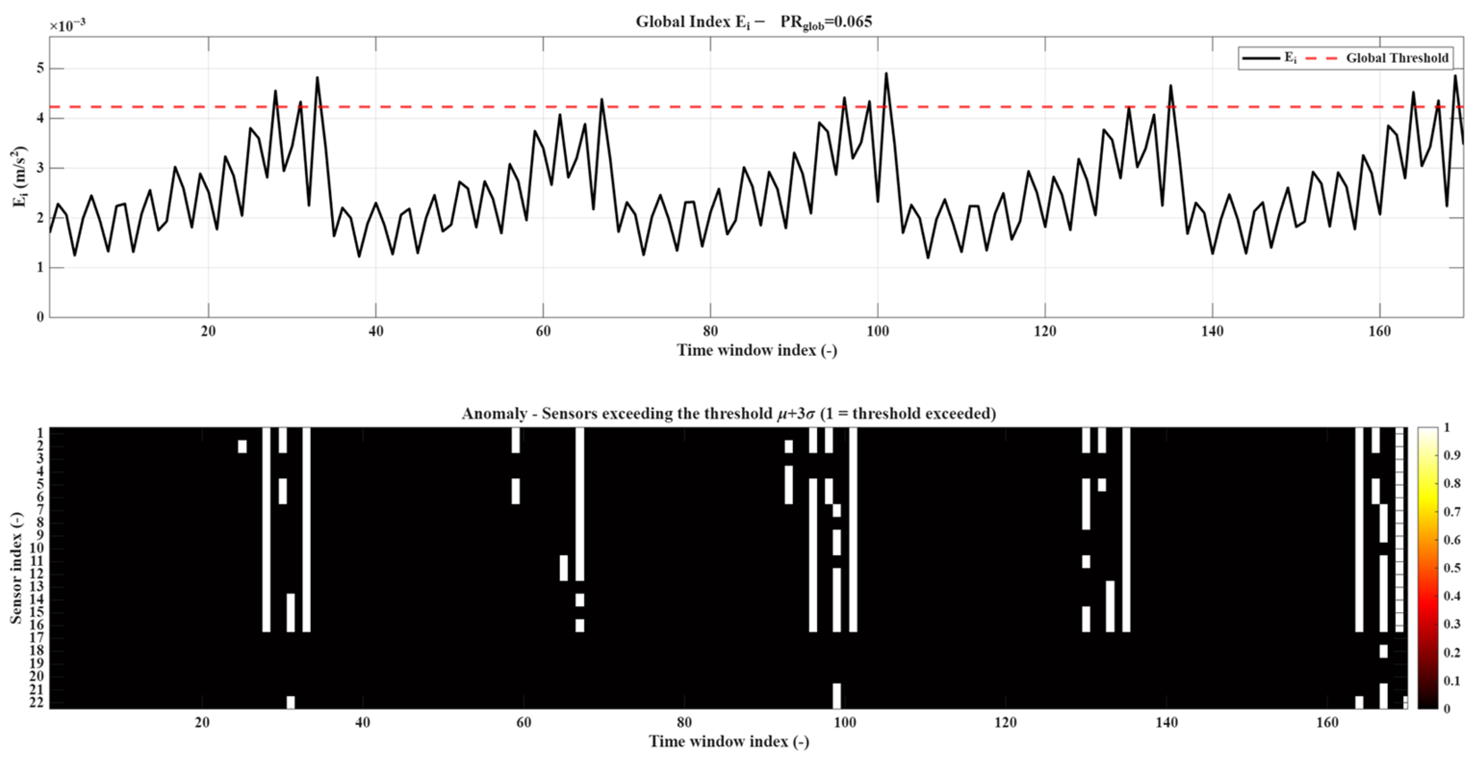
The first result, shown in Figure 8, is provided by the global reconstruction error index $E_i$, reported as a function of the time window index. As shown in the upper plot, the global error remains consistently below the global threshold identified during training, resulting in a positive rate ${\mathrm{P}\mathrm{R}}_{\mathrm{g}\mathrm{l}\mathrm{o}\mathrm{b}}=0$. Therefore, the LSTM AE does not produce false global anomaly detections under healthy conditions, despite the presence of natural variability induced by railway vehicle passages and operational excitation. Figure 8 reports the anomaly map obtained by applying the sensor-level criterion based on the three- sigma threshold ${\mu }_j+3{\sigma }_j$. Only a very limited number of isolated threshold exceedances can be observed, affecting single sensors and single time windows. These exceedances do not show temporal persistence nor spatial correlation across neighboring sensors and therefore cannot be associated with structural damage. The global anomaly index remains consistently below the detection threshold, confirming the absence of false positives at the system level. The sensor-level map shows only isolated and non-persistent threshold exceedances, indicating stable behavior of the monitored structure and robustness of the proposed method under nominal operating conditions.

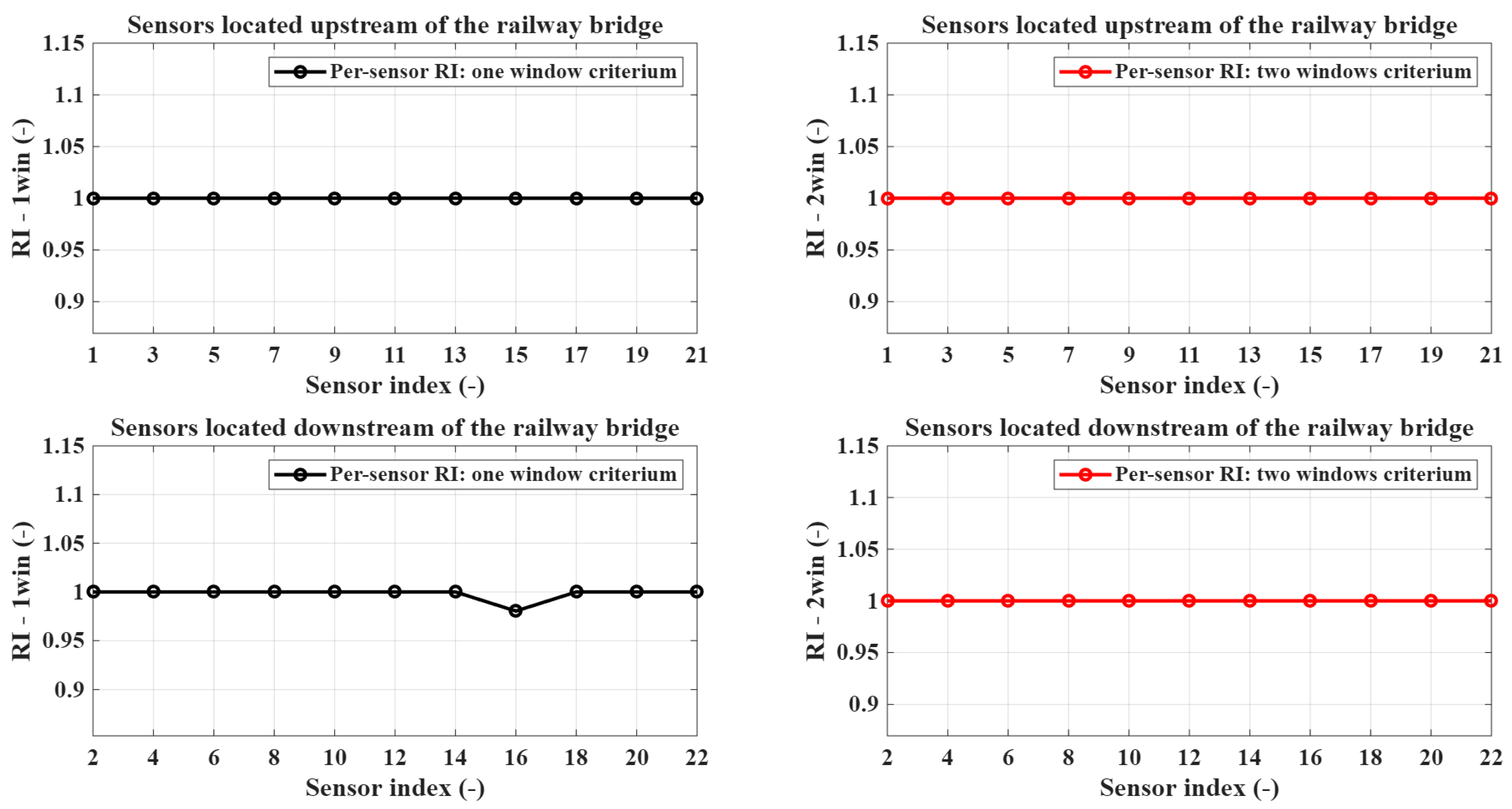
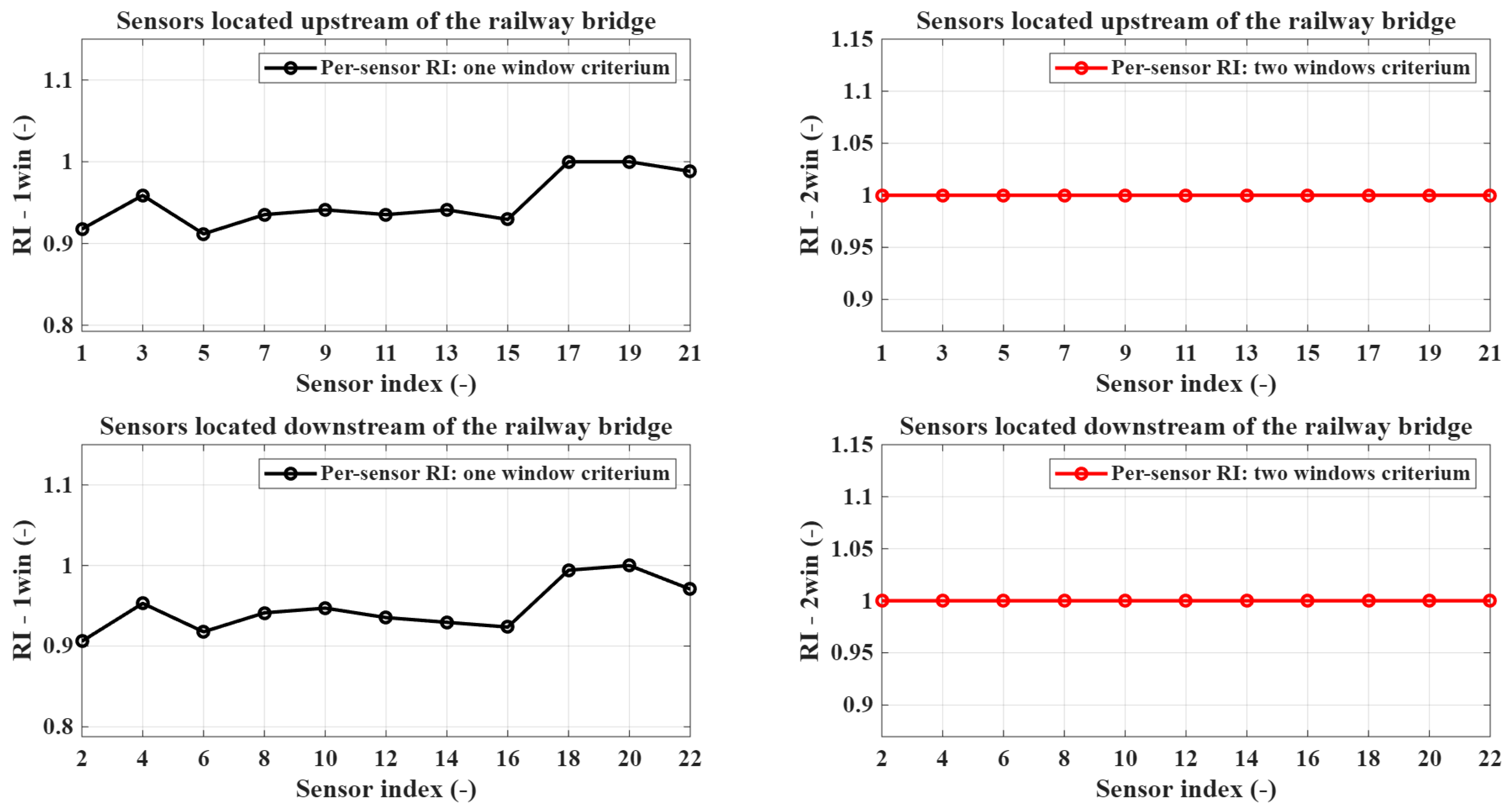
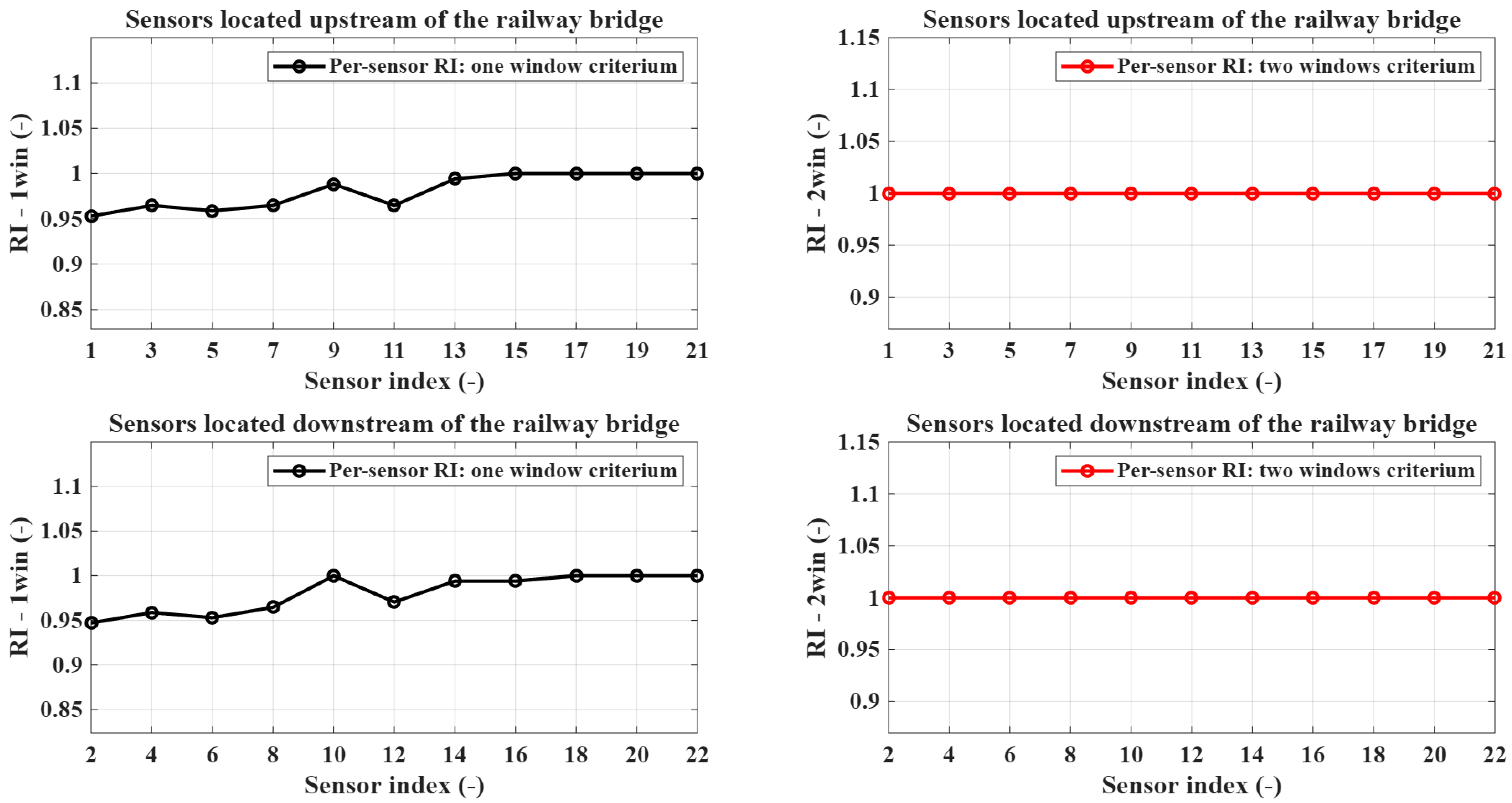
The per-sensor RI evaluated using the one-window criterion, as indicated in Equation (19), further supports this observation. For sensors located upstream of the railway bridge, the RI remains very close to unity across all sensor positions, with only marginal reductions for a limited number of sensors, as shown in Figure 9. Near-perfect RI is achieved across all sensors, confirming the absence of false anomaly detections. The two-window criterion provides fully stable classification, eliminating minor fluctuations observed in the one-window approach and enhancing the robustness of the detection framework under nominal operating conditions. A similar trend is observed for the downstream sensor line. These results indicate that the network correctly classifies healthy windows at the sensor level, with negligible false positives.

A more conservative behavior is obtained when the two-window consistency criterion is applied, as observable in Figure 9. In this case, the per-sensor RI, computed as described in Equation (22), reaches exactly 1 for both upstream and downstream sensors, meaning that no anomalies are declared when requiring two consecutive threshold exceedances. The two-window criterion effectively suppresses isolated false alarms. Furthermore, the sensitivity to persistent deviations is preserved.

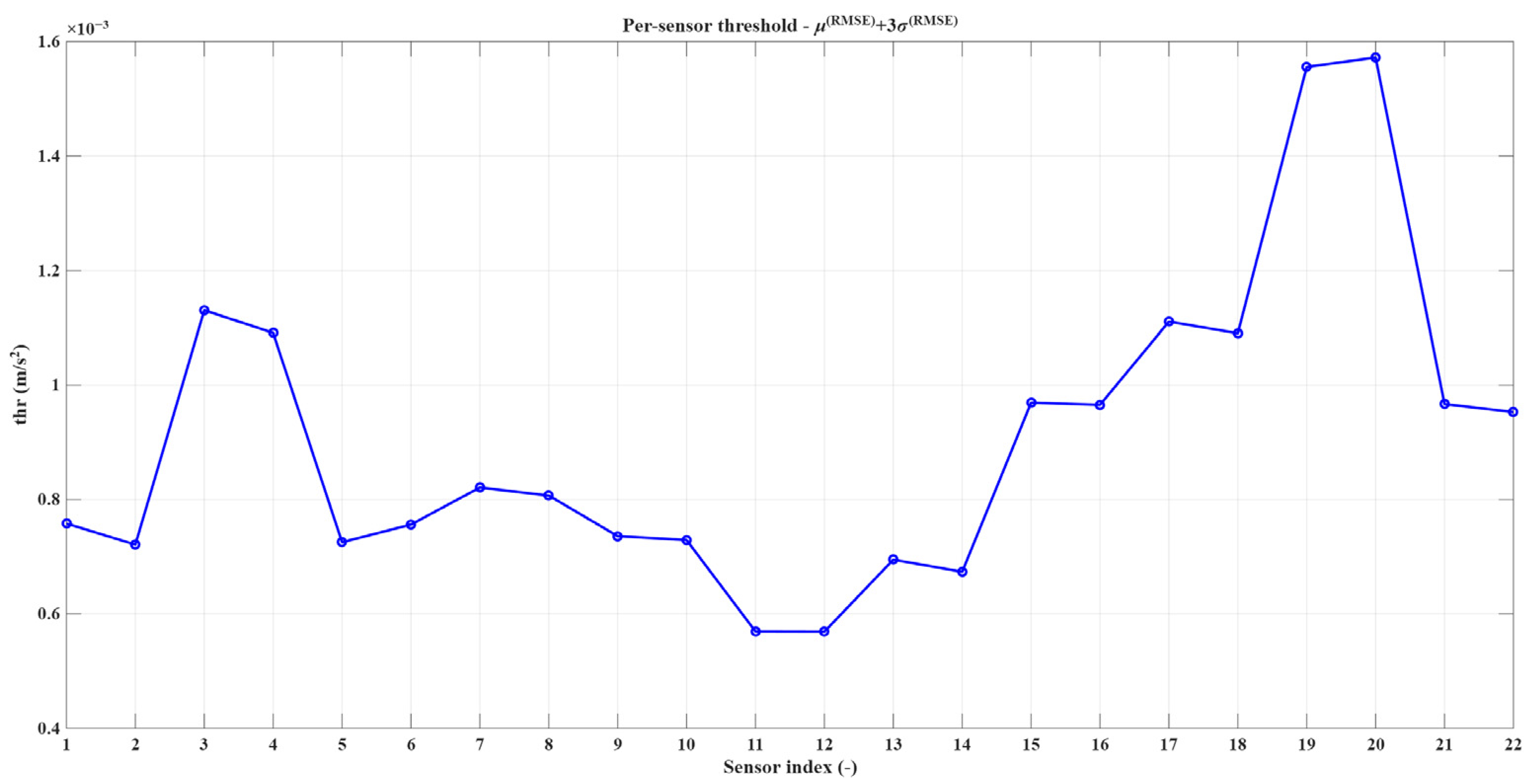
Figure 10 reports, only for the present test, the sensor-level thresholds computed as indicated in Equation (15), directly derived from the healthy-condition dataset, described in Section 4.1. The thresholds exhibit a clear spatial variability along the bridge, reflecting differences in local dynamic response, sensor position, and structural stiffness. This result highlights an important physical aspect of the proposed approach: the anomaly detection criteria are not based on uniform thresholds but are tailored to the local vibration characteristics of each sensor, thereby increasing reliability and interpretability.

The proposed framework, based on the LSTM AE, is fully consistent under healthy conditions, without introducing artificial anomalies, and provides physically meaningful thresholds usable for subsequent damage detection analyses, as demonstrated by results obtained in the H Test.

5.2. GC Test

The GC Test is aimed at assessing the capability of the trained LSTM Autoencoder to detect a mild and spatially distributed structural modification, representative of a general corrosion scenario. In this test, the railway bridge is subjected to a uniform reduction in both Young’s modulus and material density equal to 5%, affecting the entire structure.

From a physical standpoint, this type of damage is expected to induce limited variations in the global dynamic response of the bridge. Due to the distributed nature of stiffness and mass reduction and considering the overall inertial and structural characteristics of the system, no pronounced local effects are anticipated. Consequently, the bridge response remains globally coherent, and the induced damage cannot be considered critical from a structural safety perspective.

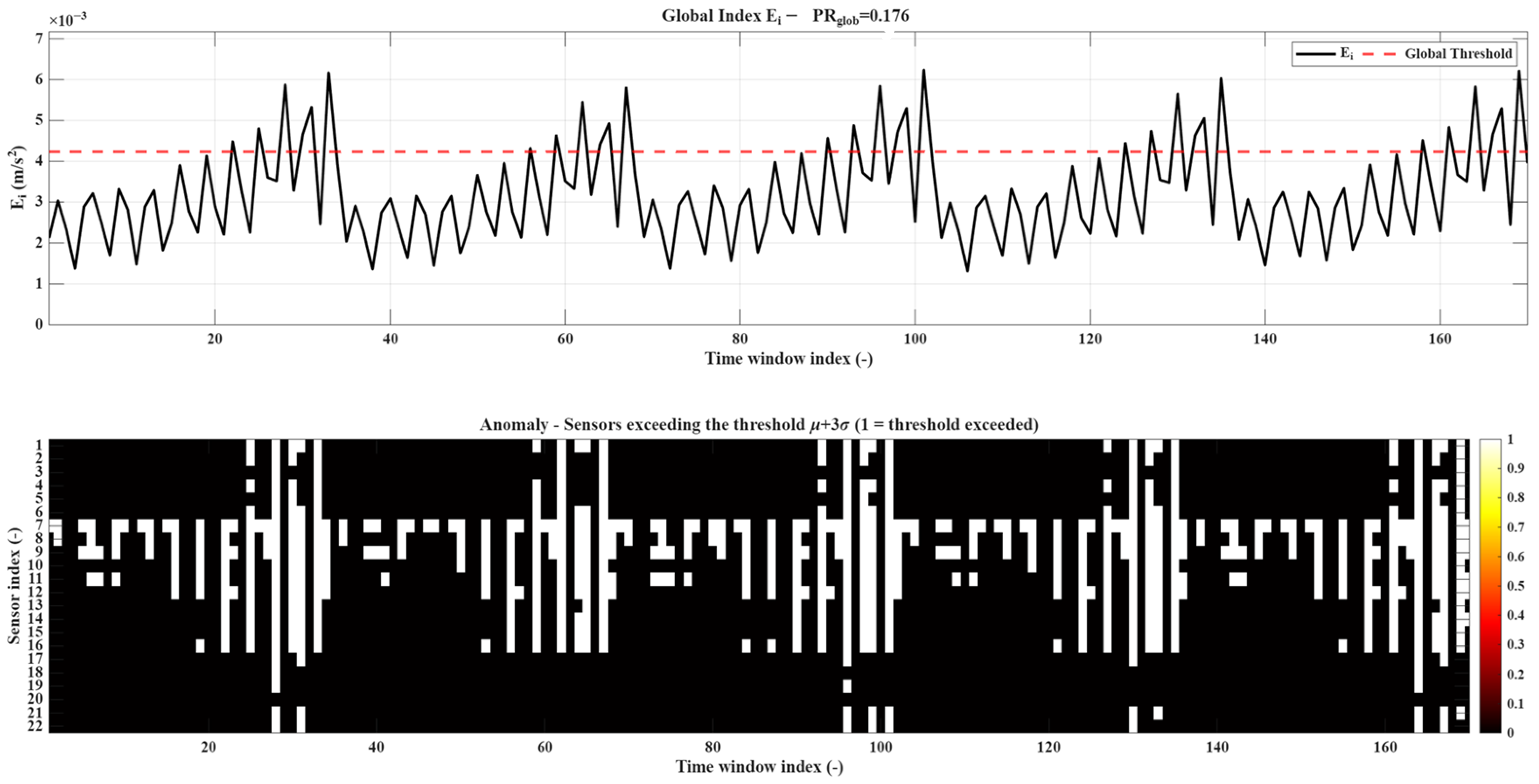
This behavior is clearly reflected in the global reconstruction error $E_i$, displayed in Figure 11. The global anomaly index frequently exceeds the detection threshold, indicating the presence of a distributed structural alteration. The sensor-level map shows widespread and persistent threshold exceedances across multiple sensors, reflecting the spatially uniform nature of the damage and confirming the capability of the proposed method to detect global changes in the structural response.

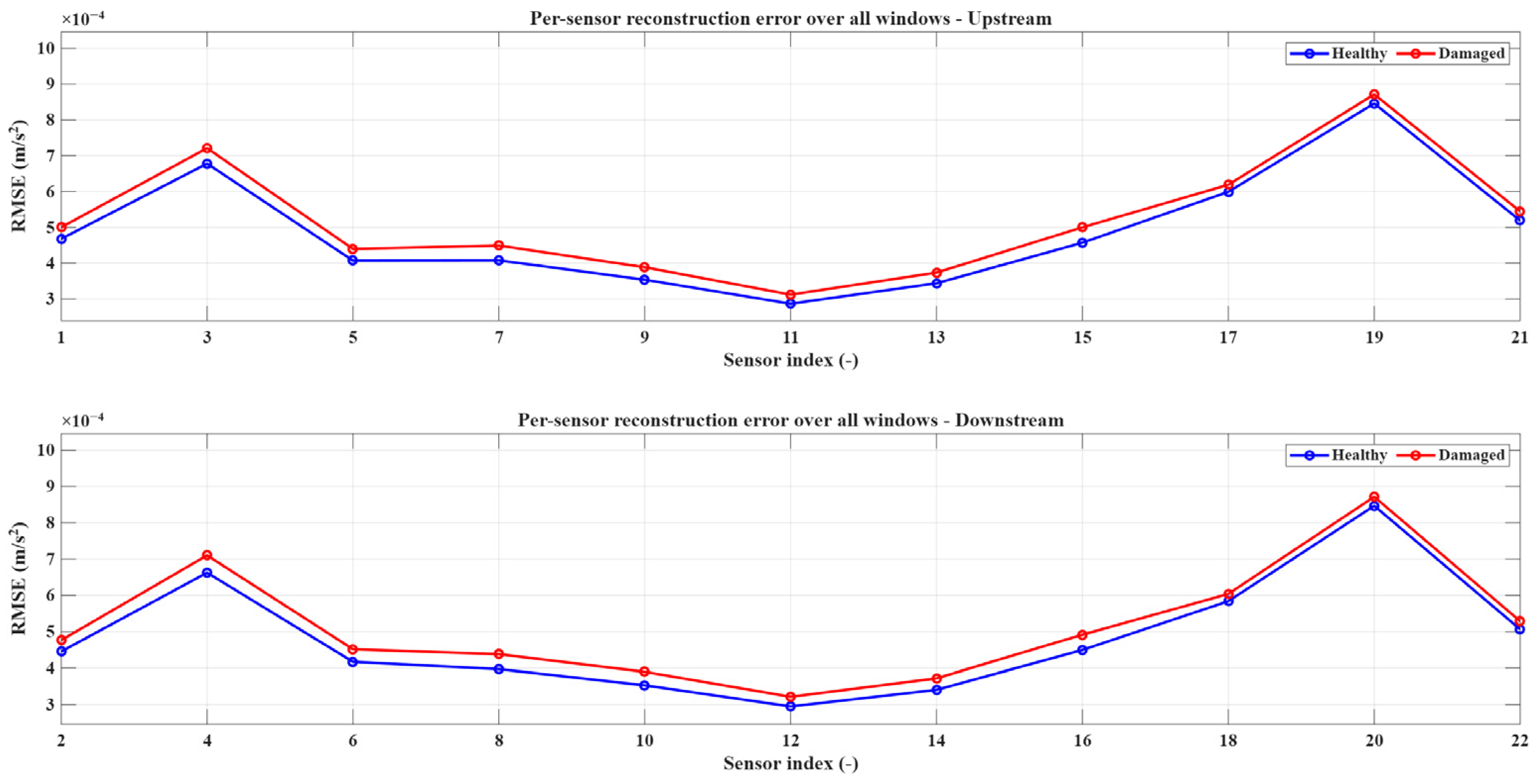
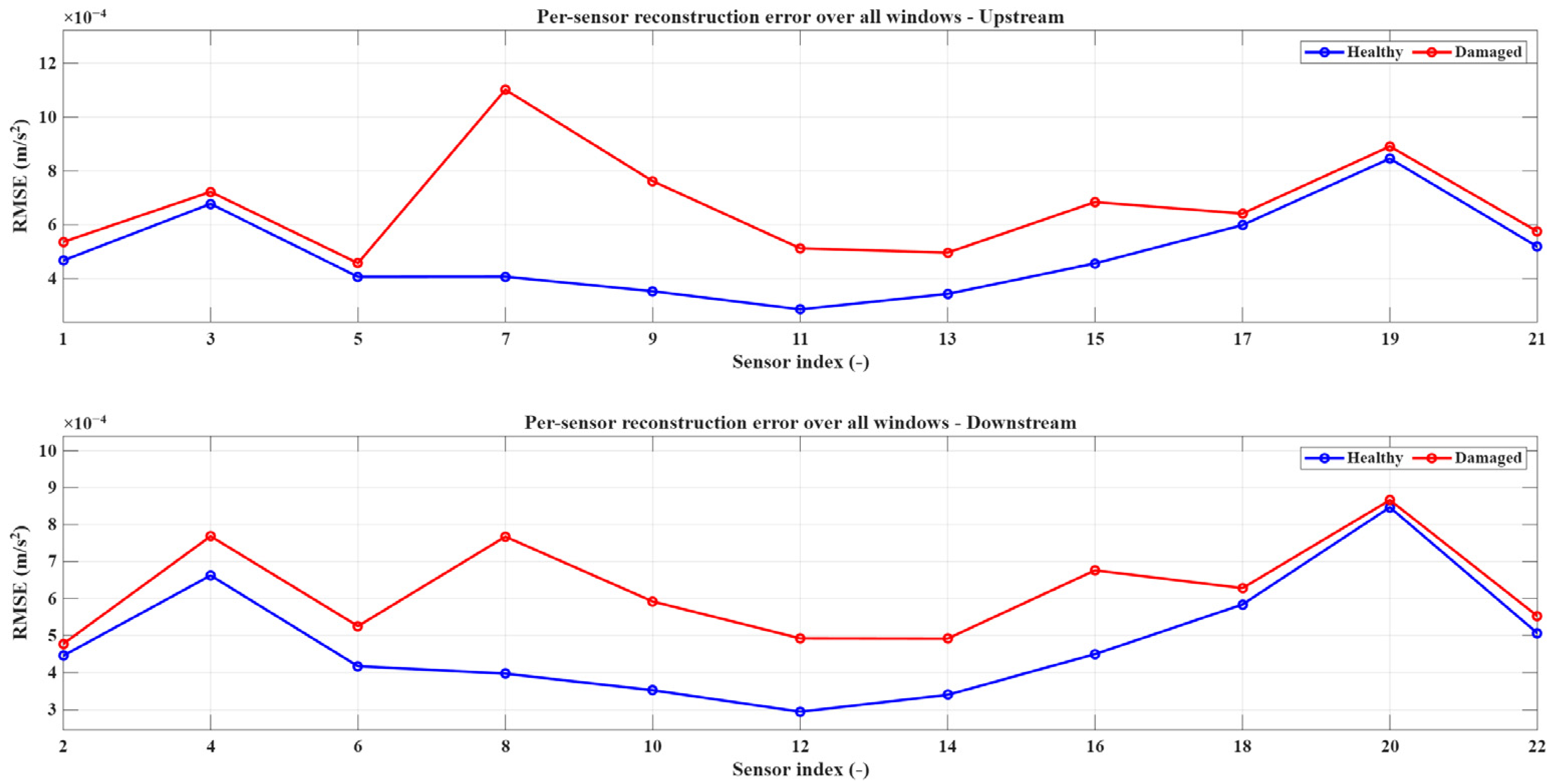
A more insightful interpretation emerges from the per-sensor reconstruction error analysis. Figure 12 shows the mean per-sensor RMSE values, separately reported for sensors located upstream and downstream of the railway bridge. An increase in reconstruction error is observed across all sensors under damaged conditions, with a consistent shift between healthy and damaged curves. The uniform distribution of the error increase confirms the spatially distributed nature of the damage and highlights the sensitivity of the proposed method to global structural alterations. Specifically, the healthy baseline has been obtained using the dataset $W_{\mathrm{healthy},\mathrm{TOT}}$, presented in Section 4.1, organized according to the sequence of time windows, shown in Figure 5, without a random permutation.

A physically meaningful signature of general corrosion is represented by the nearly constant offset between the healthy and damaged mean RMSE curves. Localized damage scenarios present sharp spatial gradients. In contrast, general corrosion is manifested as a global alteration of structural dynamics. The global damage is captured by the LSTM AE, which produces systematically higher reconstruction errors without concentrating anomalies on specific sensor locations.

The per-sensor RI values further support this interpretation. For both upstream and downstream sensors, the RI associated with the one-window criterion, shown in Figure 13, remains close to unity, with only marginal reductions. This indicates that, although the anomaly is detectable at the reconstruction error level, its intensity is not sufficient to trigger a persistent or critical degradation in detection performance. Specifically, the one-window criterion shows moderate variability across sensors, reflecting the sensitivity of the detection to distributed structural changes. In contrast, the two-window criterion provides fully stable classification with perfect RI across all sensors, demonstrating the effectiveness of temporal consistency in improving robustness for global damage detection.

By applying the stricter two-window consistency criterion, the RI reaches unity for all sensors, as shown in Figure 13, confirming the absence of a severe or alarming damage condition. The proposed LSTM AE can identify weak spatially distributed anomalies, preserving physical consistency, as demonstrated by the results of the GC Test.

5.3. LD Test10

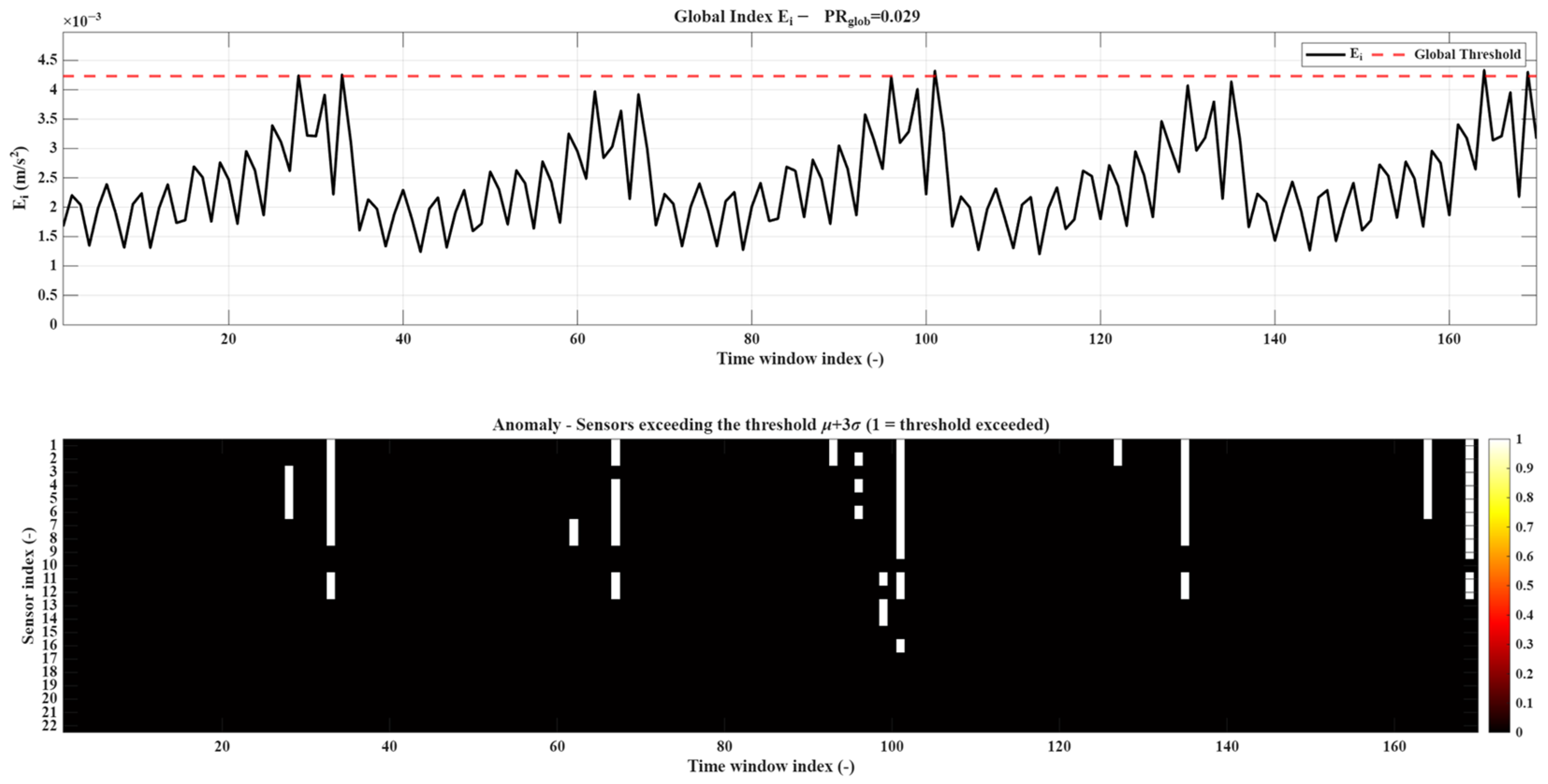
The response of the proposed anomaly detection framework, based on the LSTM AE, in the presence of a localized damage of limited severity, is investigated in the LD Test10. The damage produces only mild alterations in the global dynamic behavior of the railway bridge, due to its small extent. Therefore, the damage is weakly perceived at the structural level. The global reconstruction error $E_i$ confirms this aspect, remaining largely below the global threshold for most of the analyzed time windows, as shown in Figure 14. Only a small number of exceedances are observed, resulting in a low global positive rate, indicating that the introduced damage does not significantly compromise the overall structural response. The global anomaly index occasionally approaches or slightly exceeds the detection threshold, indicating mild and intermittent deviations from nominal behavior. The sensor-level map shows sparse and localized threshold exceedances concentrated around specific sensors, reflecting the limited spatial extent and low severity of the damage.

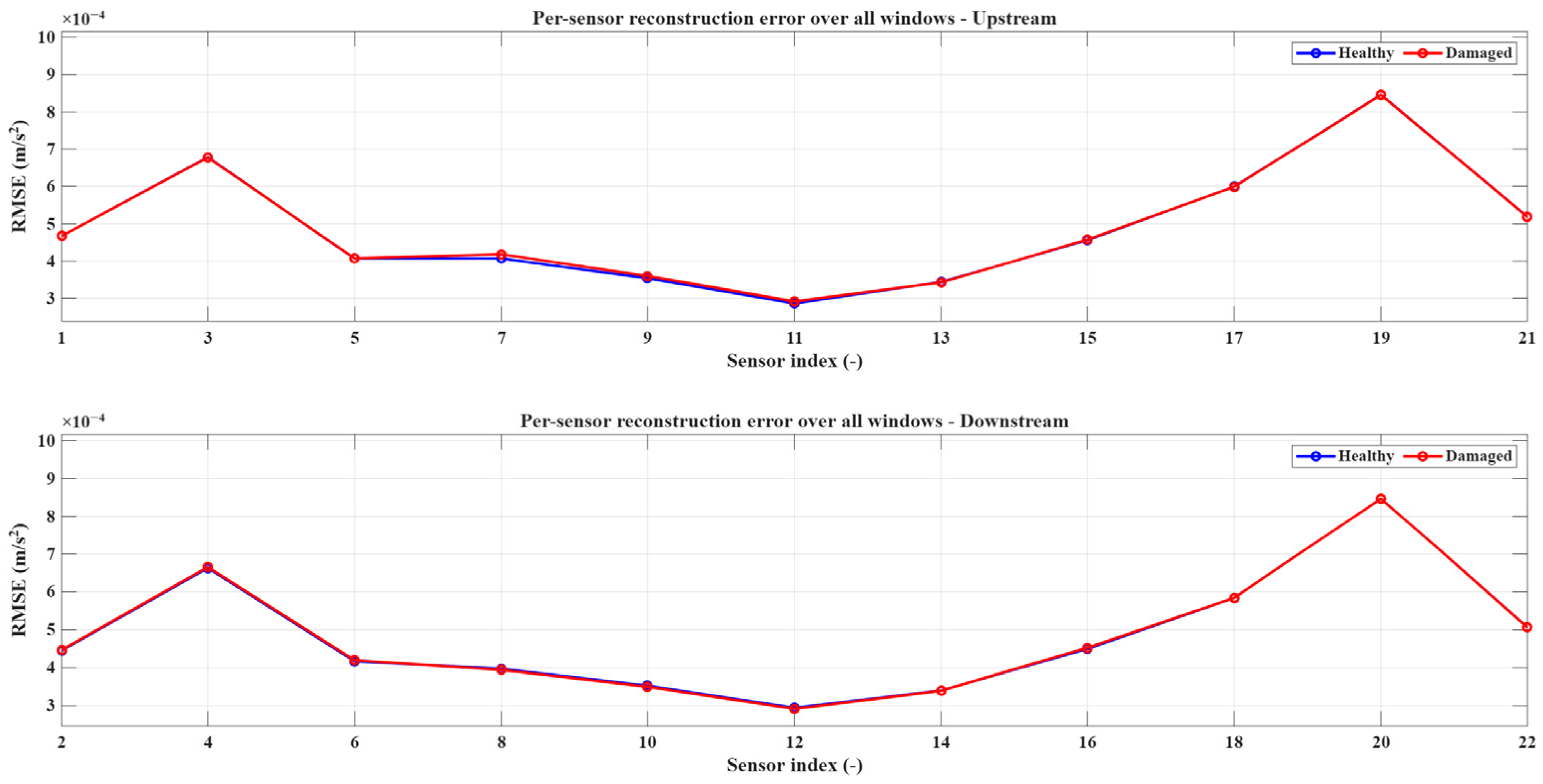
The RMSE profiles are shown in Figure 15. An increase in RMSE can be observed in correspondence with the sensors located near the damage position, with the most significant variations detected around the affected region. The other sensors, which are located away from the area near sensor 8, exhibit RMSE values of the reconstruction error comparable to healthy conditions, consistent with the localization of the damage in the structure. Furthermore, adjacent sensors are affected by the increase in reconstruction error, which is not strictly limited to a single sensor, demonstrating a consistent spatial propagation of structural vibrations. This behavior reflects the dynamic coupling of the bridge structure, where localized stiffness variations influence the response over a neighborhood of sensors. The observed pattern confirms the capability of the proposed approach to capture localized damage, preserving consistency with the underlying physical behavior of the system. This result confirms that, despite the limited severity of the damage, the proposed approach can isolate localized alterations without inducing spurious global detections.

The per-sensor RI analysis indicates high RI levels for both the one-window and two-window consistency criteria, shown in Figure 16. Minor RI reductions are observed in correspondence with the affected damaged region, while all other locations maintain values close to unity. High RI is maintained across all sensors, indicating that the mild localized damage does not significantly affect the overall detection performance. The one-window criterion shows only minor variability, while the two-window criterion ensures fully stable classification, confirming the robustness of the proposed method under low-severity damage conditions.

5.4. LD Test70

The LD Test70 scenario represents a severe localized damage condition, characterized by a pronounced stiffness and density reduction concentrated in a limited portion of the structure. Although the global dynamic response of the bridge still preserves a periodic pattern driven by train passages, the presence of damage induces clear and spatially coherent anomalies in the reconstruction error metrics.

The global reconstruction index, $E_i$, shown in Figure 17, reports a marked increase in the number of threshold exceedances compared to mild damage cases. The global anomaly index frequently exceeds the detection threshold, indicating pronounced deviations from nominal structural behavior. The sensor-level map reveals widespread and persistent threshold exceedances, particularly concentrated around the damaged region and extending to neighboring sensors, reflecting the increased severity of the damage and its broader spatial influence on the structural response.

The presence of severe local damage can be further observed in the per-sensor mean RMSE comparison presented in Figure 18. A significant offset between healthy and damaged conditions is highlighted in the region containing sensor 8, near the applied local damage. The anomaly is confined to the previously mentioned region, and not to a single sensor. This is consistent with the increased stiffness reduction, which induces a more pronounced modification of the global dynamic response of the railway bridge. The offset is sharply concentrated, consistent with the physical characteristics of a localized damage mechanism. As in the LD10 case, the highest reconstruction errors are observed in proximity to the damaged region, while adjacent sensors also exhibit elevated values due to the spatial propagation of vibrations. Furthermore, a non-uniform offset is observable, unlike global corrosion scenarios.

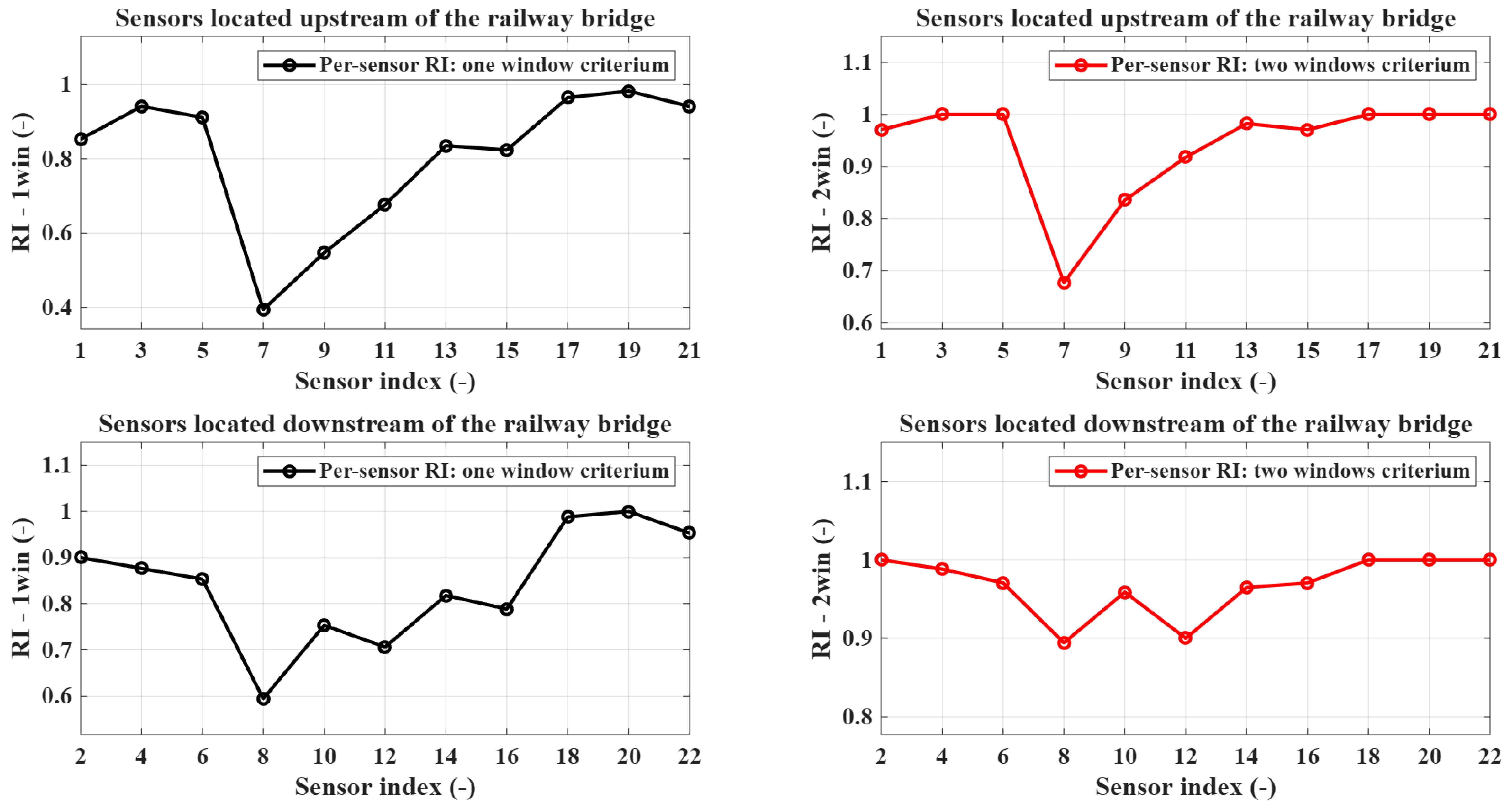
The impact of damage severity is reflected in the per-sensor RI metrics. Sensors close to the damage region exhibit a substantial drop in RI, with sensors 7 and 8 reaching the lowest values among the network, indicating a consistent classification of damaged windows as anomalous, as expected in the presence of strong local deviations, as shown in Figure 19, observing the one-window criterion.

Furthermore, a noticeable reduction in RI is highlighted at sensors 7 and 8 when applying the two-window consistency criterion, coupled with an overall RI improvement for most sensors, as shown in Figure 19, confirming both the reliability of the detection strategy and the persistence of damage-related effects.

The LSTM AE is suitable for capturing both the severity and the spatial localization of damage, as demonstrated by the LD Test70. The clear RMSE offset in the region containing sensors 7 and 8, and the coherent degradation of RI collectively indicate a physically meaningful and reliable detection of a severe localized structural anomaly. Furthermore, this behavior confirms that more pronounced damage scenarios lead to a more distributed and complex alteration of the structural dynamics, which is effectively captured by the proposed methodology.

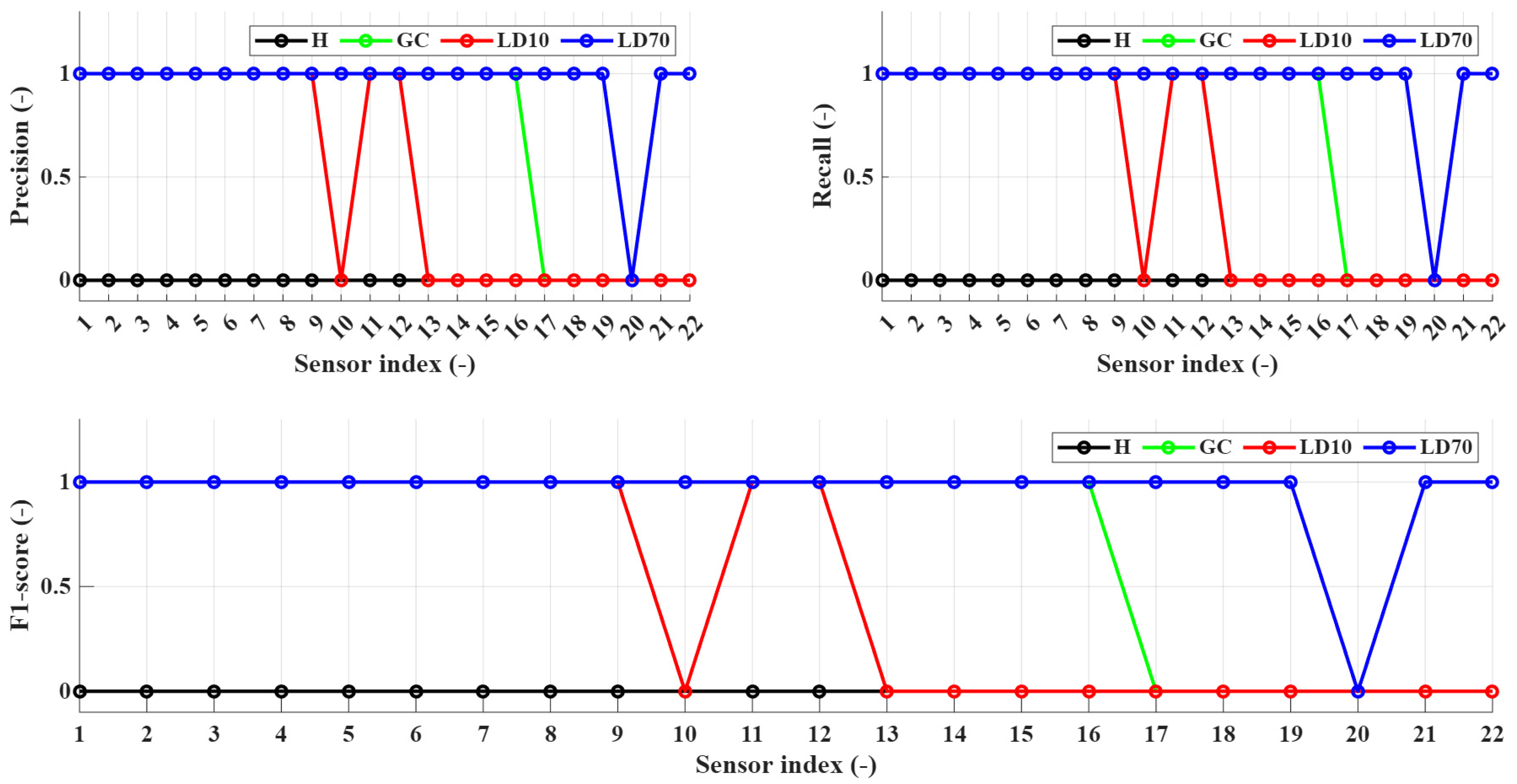
Finally, the Precision, Recall, and F1-score, computed as presented in Section 4.3, are summarized in Figure 20 for all the scenarios considered. In the present application, these metrics indicate the detectability of the damage across the sensor network, rather than their classical adoption for classification problems. The results are consistent with the trends observed in the RI-based analysis. In the healthy condition, all sensors exhibit null recall and F1-score (as there are no positives to be detected), confirming the absence of false damage detections and the reliability of the method in nominal conditions. Considering the scenarios containing information on damages, the behavior of the F1-score reflects the spatial detectability of the damage of the proposed technique. In the GC-Test, the F1-score remains close to one for almost all sensors, consistent with the uniformly distributed imposed defect represented by a general corrosion of the railway bridge. The corresponding RI values, which deviate from unity across the sensor network, are in accordance with the F1-score.

In contrast, for the LD10 scenario, the F1-score exhibits a more heterogeneous pattern, with several sensors displaying null values, consistent with the corresponding RI, where only a subset of sensors presents a significant deviation from the healthy condition. Therefore, the presence of local damage is confirmed, coupled with a weak excitation of the railway bridge, making it only partially observable. Finally, in the LD70 scenario, the F1-score confirms a nearly global detectability of the damage, with almost all sensors achieving perfect detection (F1 = 1), except for sensor 20. The related RI results are coherent with the F1-score, showing a widespread deviation from the healthy condition, indicating a clear observability of the damage across the structure. Furthermore, the RI analysis enables accurate localization of the damage, highlighting the region around sensor 8, with sensors 7 and 8 exhibiting the most significant response, as previously discussed.

The obtained results demonstrate the potential of the proposed approach under controlled simulation conditions. However, the absence of measurement noise and track irregularities represents a limitation that may affect the direct transferability of the method to real monitoring scenarios. The inclusion of the previously mentioned real-world features affecting the railway bridge and the sensing instrumentation will be considered in future studies related to the present work.

6. Conclusions

An unsupervised monitoring methodology for railway bridges based on an LSTM AE trained exclusively on healthy-condition acceleration data has been presented in this work. The methodology exploits multichannel acceleration signals, obtained from a detailed numerical model simulating the coupled train–track dynamics, and a reconstruction error-based indicator to identify deviations from nominal structural behavior. The reliability of the proposed monitoring approach in distinguishing between healthy conditions, mild global degradation, and localized damage of increasing severity has been demonstrated by the results obtained on the different test scenarios. The results obtained from the numerical simulations demonstrate that the proposed approach captures changes in the structural dynamic response through variations in reconstruction error. Particularly, the method demonstrates sensitivity to both distributed and localized damage scenarios. Furthermore, the adopted dual-threshold strategy enables distinguishing between global anomalies and sensor-level effects, confirming the suitability of the proposed approach for continuous monitoring applications, where reliability and avoidance of false alarms are essential. Overall, the proposed methodology, based on the LSTM AE, is suitable for structural health monitoring of railway bridges, representing a physically consistent, data-driven, and computationally efficient tool capable of operating under realistic operational variability, without requiring labeled damaged data or numerical model updating.

Future developments will focus on investigating more articulated and computationally efficient autoencoder architectures, aiming to enhance sensitivity to early-stage damage and reduce training and inference costs. Additionally, damage classification criteria explicitly linked to the structural characteristics of the bridge will be defined, enabling both anomaly detection and a more direct interpretation of damage type and severity within a bridge-specific diagnostic framework. Furthermore, more advanced statistical approaches related to thresholding will be explored to further improve detection robustness, including confidence interval estimation and probabilistic modeling of reconstruction errors. Finally, it is important to stress that train–track–bridge dynamic simulations will be carried out, accounting also for track geometrical profile and its evolution in time, to further investigate the robustness of the proposed approach, including validations based on experimental data collected on the monitored bridge.