Nonlinear Vibrations of Filled Re-Entrant Hexagonal Units: Coupled Geometric–Inertial Effects

Abstract

This work solves the problem associated with the lack of analytical models capable of describing the nonlinear vibration behavior of re-entrant hexagonal units when geometric nonlinearity and structural modifications, such as soft filling, are taken into account. The purpose of this study is to develop an analytical framework that enables prediction and control of vibration characteristics, with particular emphasis on achieving low-frequency response and enhanced energy storage and redistribution within the structure. The proposed approach is based on Lagrangian modeling of the unit cell, leading to a nonlinear equation of motion of the Liénard type that admits a first integral. By exploiting the existence of this integral, an approximate analytical expression for the oscillation period is derived using energy-based methods. The analysis is performed for two configurations: an empty unit and a unit filled with a soft material, allowing direct comparison of their dynamic responses. The analytical results are validated through comparison with numerical simulations and available experimental data. A parametric study is conducted to evaluate the influence of the mass ratio and the re-entrant angle on the oscillation period and frequency. Furthermore, the effects of filling mass, stiffness, and degree of filling are systematically investigated, revealing distinct inertia-dominated and stiffness-dominated regimes. The obtained results provide clear design guidelines for tailoring the dynamic response of re-entrant hexagonal units. It is shown that low-frequency vibration and increased capacity for energy storage can be achieved through appropriate selection of geometric parameters and filling properties, with potential applications in vibration control and structural design.

1. Introduction

Cellular materials with tailored mechanical properties have attracted significant attention due to their ability to achieve performance characteristics governed primarily by geometry rather than material composition. Among these, auxetic structures—characterized by a negative Poisson’s ratio—have been widely studied owing to their unusual deformation mechanisms and enhanced mechanical behavior, such as improved energy redistribution and indentation resistance. A representative class of such structures is based on re-entrant geometries, particularly re-entrant hexagonal cells, in which inwardly inclined ribs enable lateral expansion under tensile loading. The foundations for understanding the mechanical behavior of cellular systems were established in early studies on honeycomb structures [1], which demonstrated that key properties such as bending stiffness, elastic buckling, and plastic collapse are predominantly governed by structural topology. The concept of auxetic behavior was later experimentally confirmed in [2], while [3] further extended these ideas to polymeric systems and provided a systematic framework for auxetic materials design. Since then, a substantial body of research has been devoted to auxetic structures and re-entrant hexagonal configurations (see reviews [4,5,6,7,8]).

Subsequent studies have explored various geometric modifications of re-entrant cells in order to enhance their mechanical performance. For example, Ref. [9] proposed modified geometries with increased compliance, while [10,11,12,13,14] introduced alternative configurations aimed at improving stiffness and auxetic response. In parallel, experimental investigations have demonstrated that, in addition to geometry, material selection significantly influences the dynamic response of such structures, as shown for aluminum [15] and steel [16] unit cells.

Despite these advances, most research has focused on static or quasi-static analysis of auxetic and honeycomb structures [17], as well as on constitutive modeling under large deformations. In particular, Ref. [18] developed a nonlinear constitutive model that accounts for in-plane stress–strain relations, Young’s modulus, and Poisson’s ratio of auxetic honeycombs, highlighting the importance of nonlinear effects. These models have been further employed in subsequent studies such as [19]. However, geometric nonlinearity is often not fully incorporated into the analysis of dynamic behavior.

Investigations of vibration characteristics of re-entrant auxetic structures have emerged only recently. Studies such as [16] and [20] examine the dynamic response and band structure of such systems, primarily using experimental and numerical approaches. Similarly, Ref. [21] analyzed structures composed of multiple re-entrant cells under cyclic loading, showing that their response depends strongly on structural configuration. Nevertheless, a comprehensive analytical description of the nonlinear vibration behavior of a single re-entrant unit cell is still lacking.

From an application standpoint, particular attention has been devoted to enhancing energy storage capabilities. This can be achieved through geometric tailoring, such as combining conventional and auxetic cells [22], incorporating auxetic units with a damping layer [23] or employing advanced fabrication techniques, including 3D printing of cellular structures [24]. However, the relationship between structural parameters and vibration characteristics, particularly in the presence of geometric nonlinearity and structural modifications such as soft filling, remains insufficiently understood. In particular, existing studies lack explicit analytical formulations that capture the coupled effects of geometric nonlinearity and inertia in the dynamic response of a single re-entrant unit cell. As a result, the influence of nonlinear terms on key vibration characteristics, such as oscillation period and amplitude, is not yet fully clarified. Despite extensive research, there is still no explicit analytical formulation that captures the coupled effects of geometric nonlinearity and inertia in the dynamic response of a single re-entrant unit. In particular, the influence of nonlinear terms on the oscillation period and amplitude remains insufficiently understood.

Therefore, the main objective of this paper is to develop a rigorous analytical framework for the vibration analysis of a re-entrant hexagonal unit that incorporates geometric nonlinearity and soft filling. The proposed approach provides explicit expressions for the oscillation amplitude and frequency, enabling direct comparison with numerical simulations and available experimental data. Furthermore, the model allows for systematic evaluation of the influence of key parameters, offering design-oriented insights for tailoring unit cell configurations with enhanced energy storage capacity and reduced vibration frequencies. The developed analytical model thus provides a basis for understanding and predicting the nonlinear vibration behavior of re-entrant structures with practical relevance for low-frequency vibration control.

2. Materials and Research Methods

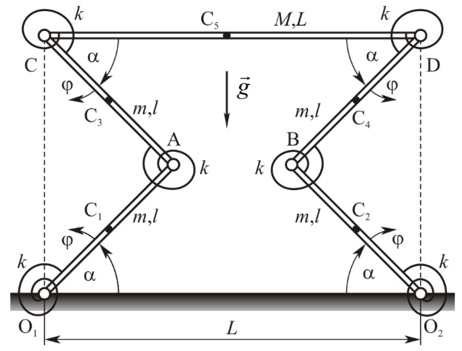
Consider a re-entrant hexagon structure shown in Figure 1. The unit is modeled as a system of six beams connected by rotational springs with finite stiffness, thereby explicitly accounting for the bending stiffness of real connections. The model represents a standard energy-consistent approximation of a continuous frame, where bending effects are lumped at the nodes. For the regular hexagon subjected to symmetric loading, the nodal rotations are inherently small due to geometric symmetry and load balance. As a consequence, the bending moments in the rotational springs remain limited, and the system response approaches that of an ideal pin-jointed structure, as long as these moments are small compared to the axial forces in the members. This approximation may become less accurate in the presence of asymmetry or near critical instability points, where nodal rotations can increase significantly.

The upper CD and lower O₁O₂ beams have the length L and mass M, while the inclined beams have equal length l and mass m. In the initial equilibrium configuration, the inclined beams form the re-entrant angle $\mathit{\alpha }$ with upper, i.e., lower beam. After initial action perpendicular on the upper beam vibration is induced in the unit. It is assumed that due to the fact that the lower beam is fixed, the motion of the upper beam is parallel to initial position while the motion of the inclined beams is symmetric.

The structure possesses one degree of freedom, and the generalized coordinate is defined as the angle $\phi$ which is the perturbation of the re-entrant angle α. Thus, during the motion the variable angle is (α + $\phi )$.

2.1. Mathematical Modeling and Governing Equations of the Re-Entrant Hexagonal Unit

The kinetic energy of the unit is the sum of the kinetic energies of bars inclined beams and of the upper beam CD. Due to the symmetry of the structure, the kinetic energies of beams O₁A and O₂B are equal, as are those of AC and BD, i.e., $T_1$=$T_2$ and $T_3$ =$T_4$, so that

$$T=2T_2+2T_4+T_5$$

(1)

Beams O₁A and O₂B undergo rotational motion, and their kinetic energy is therefore given by

$$T_2={\displaystyle \frac{1}{2}}I{\dot{\phi }}^2={\displaystyle \frac{1}{6}}m{l}^2{\dot{\phi }}^2$$

(2)

where $I=m{l}^2/3$ is the moment of inertia of the bar about the hinge point. Beams AC and BD perform planar motion; therefore, their kinetic energy is given by

$$T_4={\displaystyle \frac{1}{2}}m{v}_{C4}^2+{\displaystyle \frac{1}{2}}{I}_{C4}{\dot{\phi }}^2$$

(3)

where $v_{C4}$ is the velocity of the center $C_4$ of mass of the beam BD, and $I_{C4}={\displaystyle \frac{1}{12}}m{l}^2$ is the moment of inertia of the beam with respect to its center of mass $C_4$. For

$$x_{C4}=-({\displaystyle \frac{L}{2}}-{\displaystyle \frac{l}{2}}cos(\mathit{\alpha }+\phi )), y_{C4}={\displaystyle \frac{3l}{2}}sin\left(\mathit{\alpha }+\phi \right),$$

(4)

the velocity is

$$v_{C4}^2={\dot{x}}_{C4}^2+{\dot{y}}_{C4}^2=({\displaystyle \frac{l^2}{4}}si{n}^2(\mathit{\alpha }+\phi )+{\displaystyle \frac{9l^2}{4}}co{s}^2(\mathit{\alpha }+\phi )){\dot{\phi }}^2$$

(5)

Substituting (5) into (4) it is obtained

$$T_4={\displaystyle \frac{l^2}{8}}m(si{n}^2(\mathit{\alpha }+\phi )+9co{s}^2(\mathit{\alpha }+\phi )){\dot{\phi }}^2+{\displaystyle \frac{1}{24}}m{l}^2{\dot{\phi }}^2$$

(6)

Beam CD undergoes purely translational rectilinear motion, and its kinetic energy is given by

$$T_5={\displaystyle \frac{1}{2}}M{\dot{y}}_{C5}^2=2M{l}^{2}co{s}^2(\mathit{\alpha }+\phi ){\dot{\phi }}^2$$

(7)

where

$$y_{C5}=2l sin\left(\mathit{\alpha }+\phi \right).$$

(8)

The total kinetic energy is given by

$$T={ml}^2{\dot{\phi }}^2({\displaystyle \frac{5}{3}}+\mathit{cos}(2(\mathit{\alpha }+\phi )))+M{l}^2{\dot{\phi }}^2(1+\mathit{cos}(2(\mathit{\alpha }+\phi )))$$

(9)

The potential energy of the springs located at the joints between the beams O₁O₂ and O₁A and O₂B and also CD with AC and BD (see Figure 1) are

$$V_{0-1}=V_{0-2}=V_{3-5}=V_{4-5}={\displaystyle \frac{1}{2}}k({\phi -{\phi }_n)}^2$$

(10)

and at the joints between beams O₁A and AC and also O₂B and BD

$$V_{1-3}=V_{2-4}={\displaystyle \frac{1}{2}}k(2(\phi -{{\phi }_n))}^2$$

(11)

where the ${\phi }_n$ is the angle of the pre-stressed spring. The total potential energy of springs is

$$V_s=6 k{(-{\phi }_n+\phi )}^2$$

(12)

The potential energy due to the weight of the beams is

$$V_g=2V_{g2}+2V_{g4}+V_{g5}$$

(13)

since the potential energy of beams O₁A and AC is equal to that of bars O₂B and BD, respectively. If

$$y_{C1}=y_{C2}={\displaystyle \frac{l}{2}}\mathit{sin}(\mathit{\alpha }+\phi )$$

(14)

it follows

$$V_{g2}=V_{g1}=mg{y}_{C2}=mg{\displaystyle \frac{l}{2}}sin(\mathit{\alpha }+\phi )$$

(15)

For beams AC and BD yields

$$V_{g3}=V_{g4}=mg{y}_{C4}=mg{\displaystyle \frac{3l}{2}}sin(\mathit{\alpha }+\phi )$$

(16)

and for element CD it is

$$V_{g5}=Mg{y}_{C5}=2Mglsin(\mathit{\alpha }+\phi )$$

(17)

Substituting (15)–(17) into (13) the total gravitational potential energy is obtained

$$V_g=2(M+2m)glsin(\mathit{\alpha }+\phi )$$

(18)

According to (12) and (18) the total potential energy of the system is

$$V=V_g+V_S=6 k{(-{\phi }_n+\phi )}^2+2(M+2m)glsin(\mathit{\alpha }+\phi )$$

(19)

Using L = T − V and applying Lagrange’s equation, the governing equation is obtained

$$\begin{array}{cc}\hfill {[l}^2\left({\displaystyle \frac{10}{3}}m+2M\right)& +2(M+{m)l}^2\mathit{cos}\left(2\left(\mathit{\alpha }+\phi \right)\right)]\ddot{\phi }-2(M+{m)l}^2\mathit{sin}\left(2\left(\mathit{\alpha }+\phi \right)\right){\dot{\phi }}^2+12 k(-{\phi }_n+\phi )\hfill \\ & +2\left(M+2m\right)glcos\left(\mathit{\alpha }+\phi \right)=0\end{array}$$

(20)

The initial prestress condition gives

$${\phi }_n={\displaystyle \frac{M+2m}{6k}}gl cos\mathit{\alpha }$$

(21)

Substitution yields the final nonlinear equation

$$\begin{array}{cc}\hfill {[l}^2\left({\displaystyle \frac{10}{3}}m+2M\right)& +2(M+{m)l}^2\mathit{cos}\left(2\left(\mathit{\alpha }+\phi \right)\right)]\ddot{\phi }-2(M+{m)l}^2\mathit{sin}\left(2\left(\mathit{\alpha }+\phi \right)\right){\dot{\phi }}^2+12k\phi \hfill \\ & -4\left(M+2m\right)glsin\left(\phi +{\displaystyle \frac{\mathit{\alpha }}{2}}\right)\mathrm{s}\mathrm{i}\mathrm{n}({\displaystyle \frac{\phi }{2}})=0\hfill \end{array}$$

(22)

The nonlinear equation of motion (22), characterized by strong geometric and inertial nonlinearities, describes the motion in the vicinity of the equilibrium position. The governing equation is of Liénard-type with a quadratic velocity term and position-dependent inertia. Unlike classical formulations, the system contains nonlinear coupling between geometry, inertia, and restoring forces. Thus, the novelty of the model lies in the explicit inclusion of the effects of position-dependent inertia and allowing analytical treatment of oscillatory behavior.

2.2. Stability Analysis

For small oscillations, Equation (22) is linearized, leading to the harmonic oscillator equation with natural frequency given by

$${\mathsf{\Omega }}^2={\displaystyle \frac{6{\omega }_0^2-\left(\frac{M}{m}+2\right){\omega }_1^{2}sin\left(\frac{\mathit{\alpha }}{2}\right)}{\frac{5}{3}+\frac{M}{m}+(\frac{M}{m}+1)\mathit{cos}\left(2\mathit{\alpha }\right)}}$$

(23)

where

$${\omega }_0^2={\displaystyle \frac{k}{m{l}^2}}, {\omega }_1^2={\displaystyle \frac{g}{l}}$$

(24)

The stability of the equilibrium position is determined by the sign of Ω². The motion is stable if Ω² > 0, while Ω² < 0 corresponds to an unstable equilibrium. From Equation (23), it follows that the stability condition depends on both the mass ratio M/m and the geometric parameter represented by the angle α. In particular, a sufficient condition for stability can be obtained from the requirement Ω² > 0 in the form

$${\omega }_0^2>\left({\displaystyle \frac{M}{m}}+2\right){\displaystyle \frac{{\omega }_1^2}{6}}$$

(25)

which defines an admissible range of the mass ratio ensuring stable oscillations. This condition does not explicitly depend on the angle α and therefore represents a conservative (sufficient) estimate of the stability region. Accordingly, for

$$0<\left({\displaystyle \frac{M}{m}}\right)<6{\displaystyle \frac{{\omega }_0^2}{{\omega }_1^2}}-2$$

(26)

the equilibrium position is guaranteed to be stable. Namely, Equation (26) defines a conservative stability region independent of α.

In the following section the research methodology will consists of: (i) derivation of the nonlinear equation of motion using Lagrange’s equations, (ii) analytical reduction to a Liénard-type equation, (iii) derivation of the first integral, (iv) analytic approximation of the oscillation period, and (v) validation using numerical simulations and experimental data.

3. Analytical Reduction and Nonlinear Oscillation Analysis of the Re-Entrant Hexagonal Unit

3.1. Small-Angle Approximation and Reduced Nonlinear Model

To obtain an approximate analytical solution, simplifications are introduced in (22) under the assumption of small vibrations and a small rotation angle φ. Specifically, the trigonometric functions in (22) are expanded in a Taylor series up to second order in φ. This approximation is valid only for ∣φ∣ ≪ 1 (in radians), so that only linear and quadratic terms are retained. The simplified Equation (22) then yields

$$\begin{array}{cc}\hfill (l^2({\displaystyle \frac{10}{3}}m+2M& +2(M+m)\mathit{cos}2\mathit{\alpha })-4(M+{m)l}^2\phi sin2\mathit{\alpha })\ddot{\phi }-2(M+{m)l}^2\mathit{sin}2\mathit{\alpha }{\dot{\phi }}^2+2(6k\hfill \\ & -\left(M+2m\right)gl\mathit{sin}\left({\displaystyle \frac{\mathit{\alpha }}{2}}\right))\phi -2\left(M+2m\right)glcos\left({\displaystyle \frac{\mathit{\alpha }}{2}}\right){\phi }^2=0\hfill \end{array}$$

(27)

Geometric nonlinearity is introduced through nonlinear kinematic relations and the second-order Taylor expansion, leading to nonlinear terms in both inertia and restoring forces, including a quadratic velocity term and nonlinear stiffness.

Equation (27) represents a second-order differential equation with quadratic nonlinearity. In this section, approximate expressions for the vibration amplitude and period are derived.

REMARK: For larger amplitudes of φ (φ >1), geometric nonlinearity becomes significant, and Equation (27) no longer provides reliable results.

Unlike classical models, the derived equation admits a first integral with position-dependent inertia, which enables analytical evaluation of the oscillation period.

The reduced nonlinear Equation (23) is analyzed in the following sections.

3.2. First Integral Derivation via Liénard Transformation

For convenience, Equation (27) can be rewritten in the form $\ddot{\phi }+f\left(\phi \right){\dot{\phi }}^2+g\left(\phi \right)=0$, where

$$f\left(\phi \right)={\displaystyle \frac{-2(M+{m)l}^2\mathit{sin}2\mathit{\alpha }}{l^2(\frac{10}{3}m+2M+2(M+m)\mathit{cos}2\mathit{\alpha })-4(M+{m)l}^2\phi sin2\mathit{\alpha }}}$$

$$g\left(\phi \right)={\displaystyle \frac{2(6k-\left(M+2m\right)gl\mathit{sin}\left(\frac{\mathit{\alpha }}{2}\right))\phi -2\left(M+2m\right)glcos\left(\frac{\mathit{\alpha }}{2}\right){\phi }^2}{l^2(\frac{10}{3}m+2M+2(M+m)\mathit{cos}2\mathit{\alpha })-4(M+{m)l}^2\phi sin2\mathit{\alpha }}}$$

Introducing the new variable $v\left(\phi \right)={\dot{\phi }}^2,$ the equation transforms into a first-order linear differential equation ${\displaystyle \frac{dv}{d\phi }}+2f\left(\phi \right)v+g\left(\phi \right)=0$. The integrating factor is $\mu \left(\phi \right)=\int exp(2f\left(\phi \right))d\phi$. Multiplying the equation by μ(φ) and integrating yields the first integral $exp\left(2f(\phi )\right){\dot{\phi }}^2+2\int g\left(\phi \right)exp\left(2f(\phi \right))d\phi =K$, where K is a constant of integration. After explicit evaluation, the first integral takes the form

$${\dot{\phi }}^2={\displaystyle \frac{1}{{(P+\phi Q)}^2}}\left(K-2(PR{\displaystyle \frac{{\phi }^2}{2}}+\left(RQ+PS\right){\displaystyle \frac{{\phi }^3}{3}}+QS{\displaystyle \frac{{\phi }^4}{4}})\right)$$

(28)

where

$$P={\displaystyle \frac{5}{3}}+M/m+\left(M/m+1\right)cos(2\mathit{\alpha }), Q=-2(M/m+1)\mathrm{s}\mathrm{i}\mathrm{n}(2\mathit{\alpha })$$

$$R={\displaystyle \frac{6k/m-\left(M/m+2\right)gl\mathit{sin}\left(\frac{\mathit{\alpha }}{2}\right)}{l^2}}=6{\omega }_0^2-{\omega }_1^2\left(M/m+2\right)\mathit{sin}\left({\displaystyle \frac{\mathit{\alpha }}{2}}\right)$$

$$S=-{\displaystyle \frac{\left(\frac{M}{m}+2\right)glcos\left(\frac{\mathit{\alpha }}{2}\right)}{l^2}}=-{\omega }_1^2\left(M/m+2\right)\mathit{cos}\left({\displaystyle \frac{\mathit{\alpha }}{2}}\right)$$

(29)

The integration constant K depends on the initial conditions. For $\phi \left(0\right)=0$ and $\dot{\phi }\left(0\right)={\dot{\phi }}_0$ it follows

$$K=P^2{\dot{\phi }}_0^2$$

(30)

3.3. Energy-like Formulation and Amplitude Estimation

The obtained first integral admits a generalized energy-like interpretation. It can be written in the form

$$T_{eff}+V_{eff}=K$$

(31)

where the effective kinetic and potential energies are given by

$${T_{eff}=(P+\phi Q)}^2{\dot{\phi }}^2$$

$${V_{eff}=(P+\phi Q)}^2-2(PR{\displaystyle \frac{{\phi }^2}{2}}+\left(RQ+PS\right){\displaystyle \frac{{\phi }^3}{3}}+QS{\displaystyle \frac{{\phi }^4}{4}})$$

This formulation shows that the system is conservative in a generalized sense. The effective inertial coefficient depends on the angular position $\phi$, i.e. $I_{eff}=2$ ${(P+\phi Q)}^2$. Accordingly, the first integral represents an energy-like invariant defined in a space with a position-dependent metric. This invariant differs from the classical sum of kinetic and potential energy, confirming that the system remains conservative despite its nonstandard nonlinear structure.

3.4. Oscillation Period and Linear Limit Analysis

The method for determination of the approximate amplitude and period of vibration is based on the first integral of the system. Using the small values of rotation angle $\phi$ up to the second order and after transformation and modification of the relation (28) the expression for the approximate period of vibration is obtained as $T_p={\int }_0^{4{\phi }_m}{\displaystyle \frac{P+\phi Q}{\sqrt{K-{\phi }^{2}RP}}}d\phi$, i.e.,

$$T_p={\displaystyle \frac{4P}{\sqrt{RP}}}si{n}^{-1}\left({\phi }_m\sqrt{{\displaystyle \frac{RP}{K}}}\right)+{\displaystyle \frac{4Q}{RP}}(\sqrt{K}-\sqrt{K-{\phi }_m^{2}RP})$$

(32)

${\phi }_m$ is the approximate value of the maximal amplitude of vibration which satisfies the relation (28) for $\dot{\phi }=0$, i.e.,

$$K-2\left(PR{\displaystyle \frac{{\phi }_m^2}{2}}+\left(RQ+PS\right){\displaystyle \frac{{\phi }_m^3}{3}}+QS{\displaystyle \frac{{\phi }_m^4}{4}}\right)=0$$

(33)

For the case of small vibrations the approximate value of the amplitude (29) is

$${\phi }_m\approx \sqrt{{\displaystyle \frac{K}{PR}}}={\dot{\phi }}_0\sqrt{P/R}$$

(34)

and the corresponding approximate period (32) is

$$T_p=T_l-T_c$$

(35)

where

$$T_l=2\pi \sqrt{{\displaystyle \frac{\frac{5}{3}+M/m+\left(M/m+1\right)cos(2\mathit{\alpha })}{6{\omega }_0^2-{\omega }_1^2\left(M/m+2\right)\mathit{sin}\left(\frac{\mathit{\alpha }}{2}\right)}}},$$

(36)

$$T_c={\displaystyle \frac{8{\dot{\phi }}_0(M/m+1)\mathit{sin}(2\mathit{\alpha })}{6{\omega }_0^2-{\omega }_1^2\left(M/m+2\right)\mathit{sin}\left(\frac{\mathit{\alpha }}{2}\right)}}$$

(37)

$T_l$ is the period of vibration of the linearized model of unit (36), while $T_c$ represents the correction to the period due to nonlinearity (37). It is evident that the vibration period given by Equation (35) depends on the mass ratio ${\displaystyle \frac{M}{m}},$ re-entrant angle $\mathit{\alpha },$ stiffness coefficient k, and segment length l. In the following, the influence of each parameter is analyzed.

3.4.1. Linearized Oscillation Characteristics

For the linear case the period of vibration is independent on the initial values and has the form (36). Using Equation (34) and the theory of harmonic oscillator the maximal amplitude of vibration is

$${\phi }_{ml}={\dot{\phi }}_0{T}_l/2\pi$$

(38)

Analyzing (36) and (38), the vibration properties of the linearized model of the re-entrant hexagonal unit follow as

(a)

By increasing of ($M/m)$ the period of vibration is also increasing.

(b)

For $0<\mathit{\alpha }\le {\displaystyle \frac{\pi }{4}},$ the value of trigonometric functions are $1>cos$($2\mathit{\alpha })\ge 0$, and $0<\mathit{sin}\left({\displaystyle \frac{\mathit{\alpha }}{2}}\right)\le {sin}^{-1}({\displaystyle \frac{\pi }{8}})$. If ${\omega }_0^2\gg {\omega }_1^2$ the period $T_a$ is longer for smaller vales of $\mathit{\alpha }$ than those up to ${\displaystyle \frac{\pi }{4}}.$ Namely, for $\mathit{\alpha }\to 0$ it is $T_a\to 2\pi \sqrt{{\displaystyle \frac{\frac{8}{3}+2(\frac{M}{m})}{6{\omega }_0^2}}}$ and for $\mathit{\alpha }={\displaystyle \frac{\pi }{4}}$ the period is $T_a=2\pi \sqrt{{\displaystyle \frac{\frac{5}{3}+M/m}{6{\omega }_0^2-{\omega }_1^2\left(M/m+2\right){sin}^{-1}(\frac{\pi }{8})}}}$.

(c)

For the special case when $6{\omega }_0^2={\omega }_1^2\left(M/m+2\right)\mathit{sin}\left({\displaystyle \frac{\mathit{\alpha }}{2}}\right)$ the period of vibration tends to infinity, i.e. $T_a\to \infty$ and the frequency of vibration is zero.

(d)

If ${\displaystyle \frac{\pi }{4}}<\mathit{\alpha }\le {\displaystyle \frac{\pi }{2}},$ the value of trigonometric functions are $0>cos$($2\mathit{\alpha })\ge -1$, and ${\mathit{sin}}^{-1}({\displaystyle \frac{\pi }{8}})<\mathit{sin}\left({\displaystyle \frac{\mathit{\alpha }}{2}}\right)\le {\displaystyle \frac{\sqrt{2}}{2}}$. If ${\omega }_0^2\gg {\omega }_1^2$ the period $T_a$ is decreasing up to $T_a=2\pi \sqrt{{\displaystyle \frac{\frac{5}{3}}{6{\omega }_0^2-{\omega }_1^2\left(M/m+2\right)\frac{\sqrt{2}}{2}}}}$ when $\mathit{\alpha }$ tends to ${\displaystyle \frac{\pi }{2}}.$

3.4.2. Special Case: Horizontal Motion (ω₁ = 0)

For the case when the motion is in the horizontal plane and ${\omega }_1^2=0$ the period of vibration (32) simplifies into

$$T_p={\displaystyle \frac{2\pi }{{\omega }_0}}\sqrt{{\displaystyle \frac{P}{6}}}-{\dot{\phi }}_0{\displaystyle \frac{\left(\frac{M}{m}+1\right)\mathit{sin}\left(2\mathit{\alpha }\right)}{3{\pi }^2}}({{\displaystyle \frac{2\pi }{{\omega }_0}})}^2$$

(39)

The term $\sqrt{{\displaystyle \frac{P}{6}}}$ represents the correction factor for the period of vibration of the linear model. In addition, the period of vibration (39) of the unit in horizontal plane is directly proportional to the initial angular velocity.

For the linear case, an increase in the mass ratio leads to higher inertia, which directly increases the oscillation period. Conversely, increasing the re-entrant angle enhances the structural stiffness, resulting in higher frequencies and shorter periods.

4. Results and Discussion

In this section, the analytical results are systematically validated through comparisons with numerical simulations and available experimental data. The objective is to assess the accuracy of the proposed model and to analyze the influence of key parameters on the vibration characteristics.

4.1. Validation Against Numerical Results

To validate the theoretical considerations presented in Section 3, the analytical solutions are compared with high-fidelity numerical solutions obtained by solving the differential equation of motion (22).

The selection of the model parameters used in the numerical analysis is based on physically representative engineering ranges relevant to re-entrant cellular structures. In particular, the mass ratio M/m is chosen to cover both light and heavy secondary mass contributions, enabling the investigation of inertia-dominated and stiffness-dominated regimes. The parameter ${\omega }_0^2$ is selected to represent typical stiffness levels of the re-entrant frame obtained from its geometric and material properties. The considered range of parameters is therefore not arbitrary, but is intended to ensure a comprehensive analysis of the dynamic response across practically relevant operating conditions. This approach allows for a systematic evaluation of the influence of key physical parameters on the vibration characteristics of the system. This approach provides a systematic framework for analyzing the influence of key physical parameters on the vibration characteristics of the system. 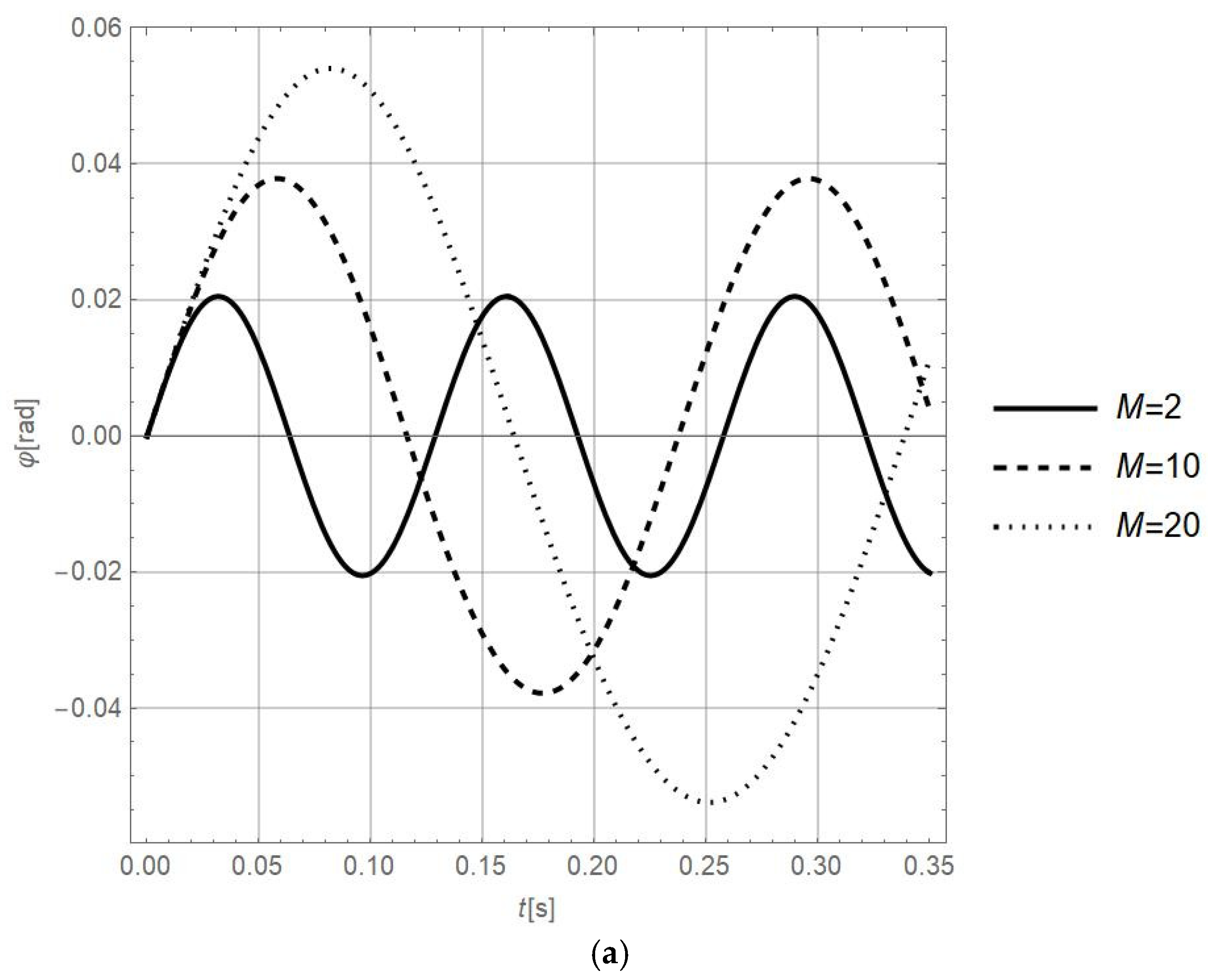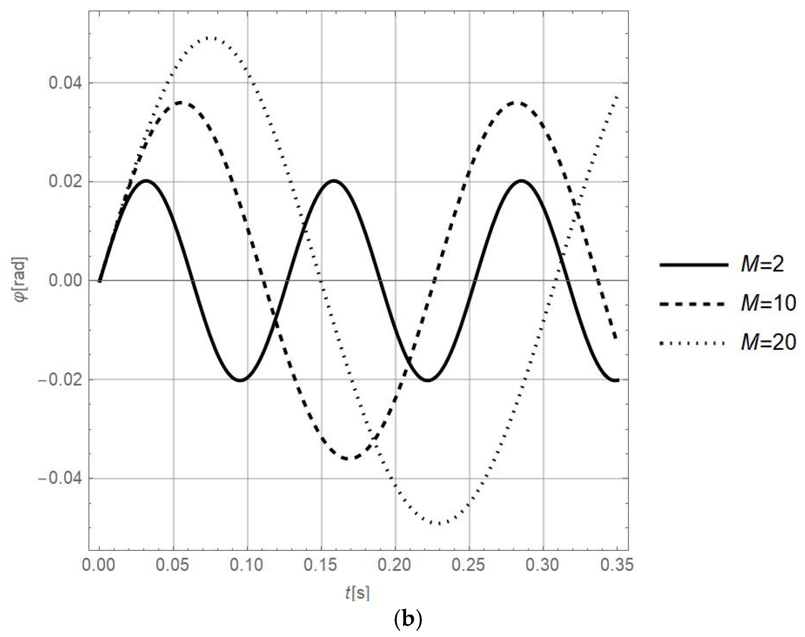The corresponding time histories φ(t) are presented in Figure 2, obtained by solving the governing equation for the parameters $\mathit{\alpha }=\pi /4,$ m = 1, ${\omega }_0^2=1500,$ and two representative values for ${\omega }_1^2$ (100 and 0), with initial conditions $\phi \left(0\right)=0, \dot{\phi }\left(0\right)=1$. The results are presented for different values of the mass M$.$

From Figure 2, it is evident that both the vibration amplitude and the period of vibration increase with increasing mass M, independently on the value of ${\omega }_1^2$. However, the amplitude is higher and the period is longer for ${\omega }_1^2$ = 100 than for ${\omega }_1^2$= 0. This statement agrees with the conclusions presented in Section 3 based on analysis of the expression (31).

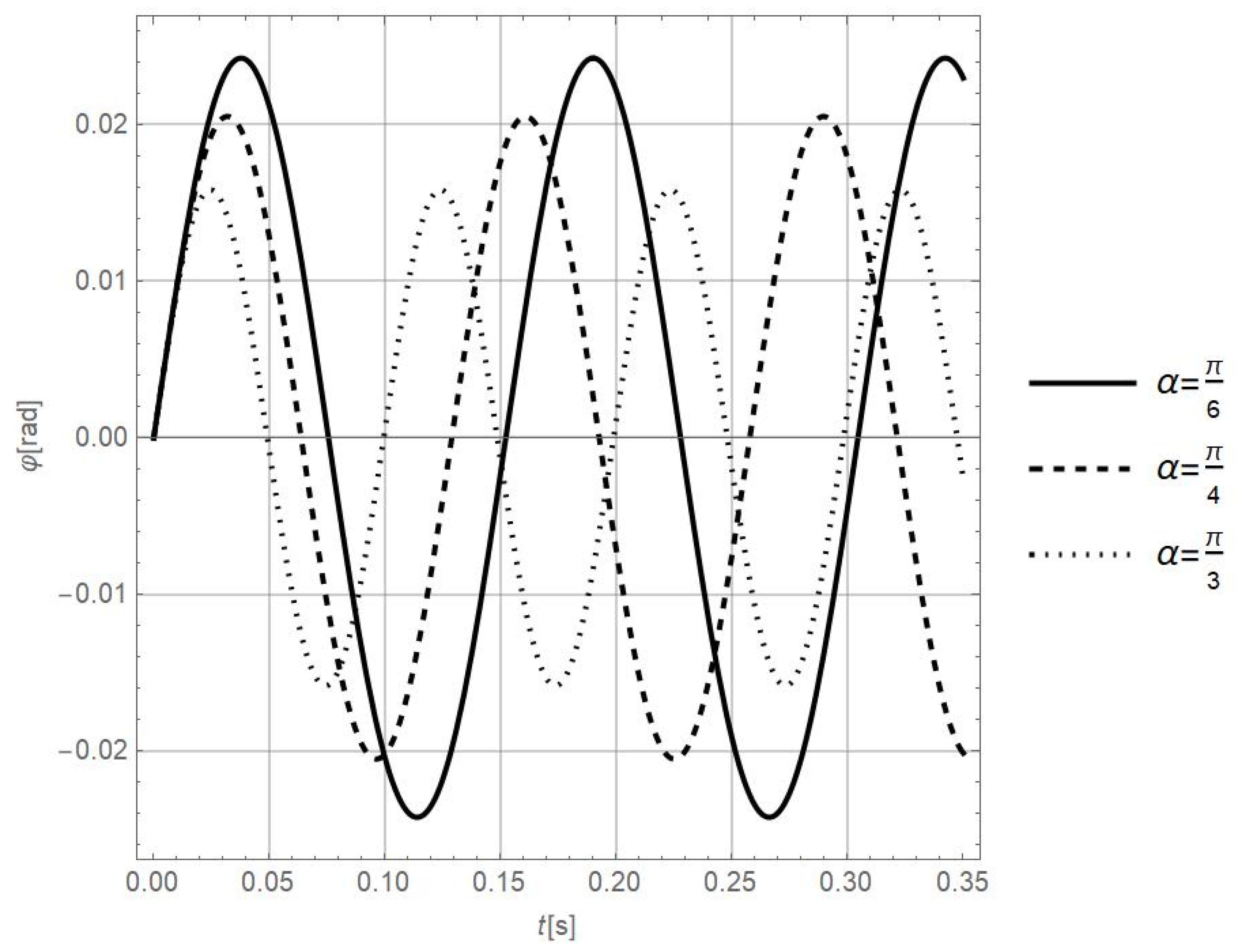
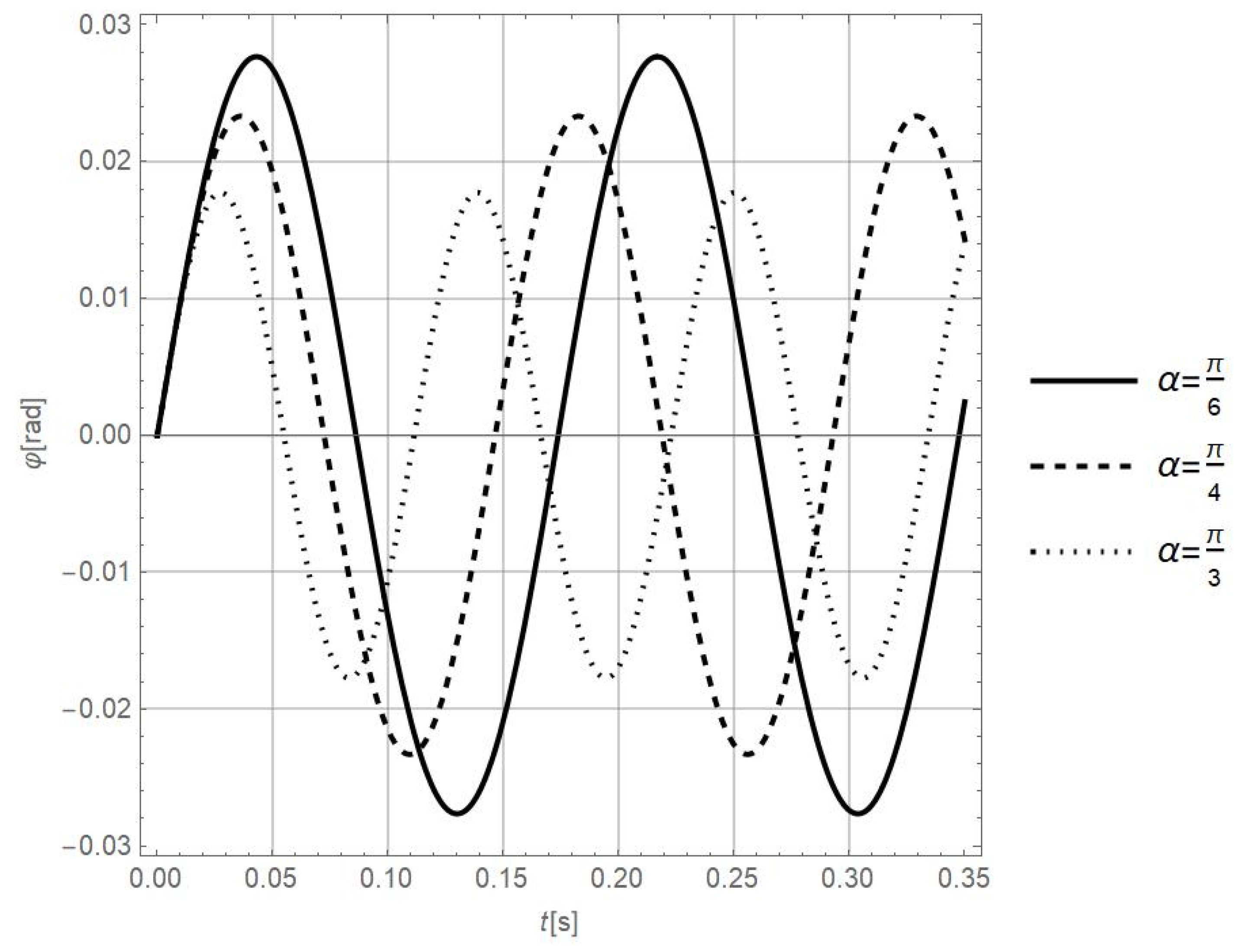
Equation (22) is numerically solved for m = 1, M = 2, ${\omega }_0^2=1500,$ and ${\omega }_1^2=100$, initial conditions $\phi \left(0\right)=0,$ and $\dot{\phi }\left(0\right)=1$, and various values of α and the results are plotted in Figure 3. As shown in Figure 3, increasing the angle α leads to a decrease in both vibration amplitude and oscillation period. This finding is also in agreement with the analytical results presented in Section 3.

To provide a fully accurate assessment of the analytical solving procedure developed in the paper, the amplitudes ${\phi }_{mn}$ and oscillation periods $T_n$ obtained numerically by solving Equation (22), as well as those determined analytically for the nonlinear system, ${\phi }_m$ (34) and $T_p$ (35), and for the linearized oscillator, ${\phi }_{ml}$ (38) and $T_l$ (36) are presented in

Table 1. Comparison of vibration amplitudes and periods obtained by numerical, analytical, and linearized models.

$\mathit{M}/\mathit{m}$	$\mathit{\alpha }$	${\mathit{\omega }}_0^2$	${\mathit{\omega }}_1^2$	${\mathit{T}}_{\mathit{n}}$	${\mathit{\phi }}_{\mathit{m}\mathit{n}}$	${\mathit{T}}_{\mathit{p}}$	${\mathit{\phi }}_{\mathit{m}}$	${\mathit{T}}_{\mathit{l}}$	${\mathit{\phi }}_{\mathit{m}\mathit{l}}$
2	$\pi /4$	1500	100	0.12790	0.02059	0.12770	0.02033	0.12498	0.02018
10	$\pi /4$	1500	100	0.23212	0.03793	0.23207	0.03694	0.22169	0.03600
20	$\pi /4$	1500	100	0.32352	0.05365	0.32359	0.05153	0.30294	0.04965
2	$\pi /6$	1500	100	0.15140	0.02431	0.15124	0.02408	0.14890	0.02371
2	$\pi /3$	1500	100	0.09858	0.01589	0.09839	0.01567	0.09603	0.01529
2	$\pi /4$	1500	0	0.12681	0.02018	0.12675	0.02018	0.12408	0.01976
10	$\pi /4$	1500	0	0.22615	0.03600	0.22605	0.03600	0.21633	0.03447
20	$\pi /4$	1500	0	0.30811	0.04965	0.30813	0.04906	0.28946	0.04609

. Table 1 summarizes the vibration amplitudes and oscillation periods obtained from numerical simulations, the nonlinear analytical model, and the linearized approximation. The parameters included are the mass ratio M/m, re-entrant angle α, and angular frequencies ${\omega }_0$ and ${\omega }_1$. The deviation between the analytical and numerical results is negligible, indicating excellent agreement. In contrast, the linearized model shows small deviations (below 10%), which remain acceptable for engineering applications.

4.2. Validation Against Experimental Data

To further validate the proposed model, the analytical predictions are compared with experimental data reported in [16]. In [16], a re-entrant hexagonal unit-cell frame, corresponding to the model shown in Figure 1, was experimentally investigated. The unit was constructed from six beams with square cross-sections of 4 mm × 4 mm, 8 mm × 8 mm, 12 mm × 12 mm, and 16 mm × 16 mm. The structure was made of steel with density ρ = 7850 kg/m³ and Young’s modulus E = 2 × 10¹¹ Pa. The overall dimensions of the frame were 400 mm × 400 mm. The re-entrant angle of the unit frame is varied from values which correspond to auxetic structure (0 < α < π/2) up to the straight configuration (α = π/2).

In

Table 2. Analytical ($f_l)$ and experimental ($f_e$) vibration frequencies for the steel frame.

$\mathit{\alpha }$	$\mathit{a} (\mathbf{m})$	${\mathit{\omega }}_0^2$ (rad/s)	${\mathit{T}}_{\mathit{l}} (\mathbf{s})$	${\mathit{f}}_{\mathit{l}}$ (Hz)	${\mathit{f}}_{\mathit{e}}$ (Hz)
$\pi /3$	0.004	163	0.0203	$18.54$	18.95
	0.008	359	0.0092	40.83	39.63
	0.012	540	0.0061	61.42	62.59
	0.016	719	0.0046	81.78	88.24
$5\pi /12$	0.004	163	0.0151	19.58	19.59
	0.008	359	0.0069	43.14	40.57
	0.012	540	0.0046	64.89	63.34
	0.016	719	0.0034	86.41	88.13

, the experimentally obtained frequencies $f_e$ for α = π/3 and α = 5π/12 presented in [16] are compared with the frequencies computed according to Equation (36), i.e. $f_l={\displaystyle \frac{1}{T_l}}.$ The columns in Table 2 are: the re-entrant angle $\mathit{\alpha }$, cross-section dimension of the beam a, angular frequency ${\omega }_0$, approximate period of vibration $T_l$, approximate frequency $f_l$ and experimental frequency of vibration $f_e$.

The comparison leads to the following observations:

-

The relative error of the analytical predictions remains within 10%, with slightly larger deviations for higher values of α;

-

The analytical model accurately reproduces the experimentally observed trends;

-

The vibration frequency increases with both the re-entrant angle α and the cross-sectional dimension a.

Based on these conclusions, it follows that the analytical expression (36) enables the prediction of the period and frequency of small oscillations for arbitrary values of the dimensional parameter a, the re-entrant angle α, and the mass ratio M/m.

4.3. Parametric Analysis of Vibration Characteristics

Table 3. Computed vibration frequencies for M/m = 1 as a function of a and $\mathit{\alpha }$ for a steel frame.

$\mathit{\alpha }$	$\mathit{a} (\mathbf{m})$	${\mathit{\omega }}_0^2$ (rad/s)	${\mathit{T}}_{\mathit{l}} (\mathbf{s})$	${\mathit{f}}_{\mathit{l}}$ (Hz)
$\pi /6$	0.004	163	0.0307	33,2
	0.008	359	0.0139	73.2
	0.012	540	0.0092	110
	0.016	719	0.0063	146
$\pi /4$	0.004	163	0.0128	39.0
	0.008	359	0.0058	85.6
	0.012	540	0.0039	129
	0.016	719	0.0029	171
$\pi /3$	0.004	163	0.0203	49.3
	0.008	359	0.0092	108.5
	0.012	540	0.0061	163.1
	0.016	719	0.0046	217.4
$\pi /2$	0.004	163	0.0128	78.0
	0.008	359	0.0058	171.3
	0.012	540	0.0039	258.0
	0.016	719	0.0029	342.0

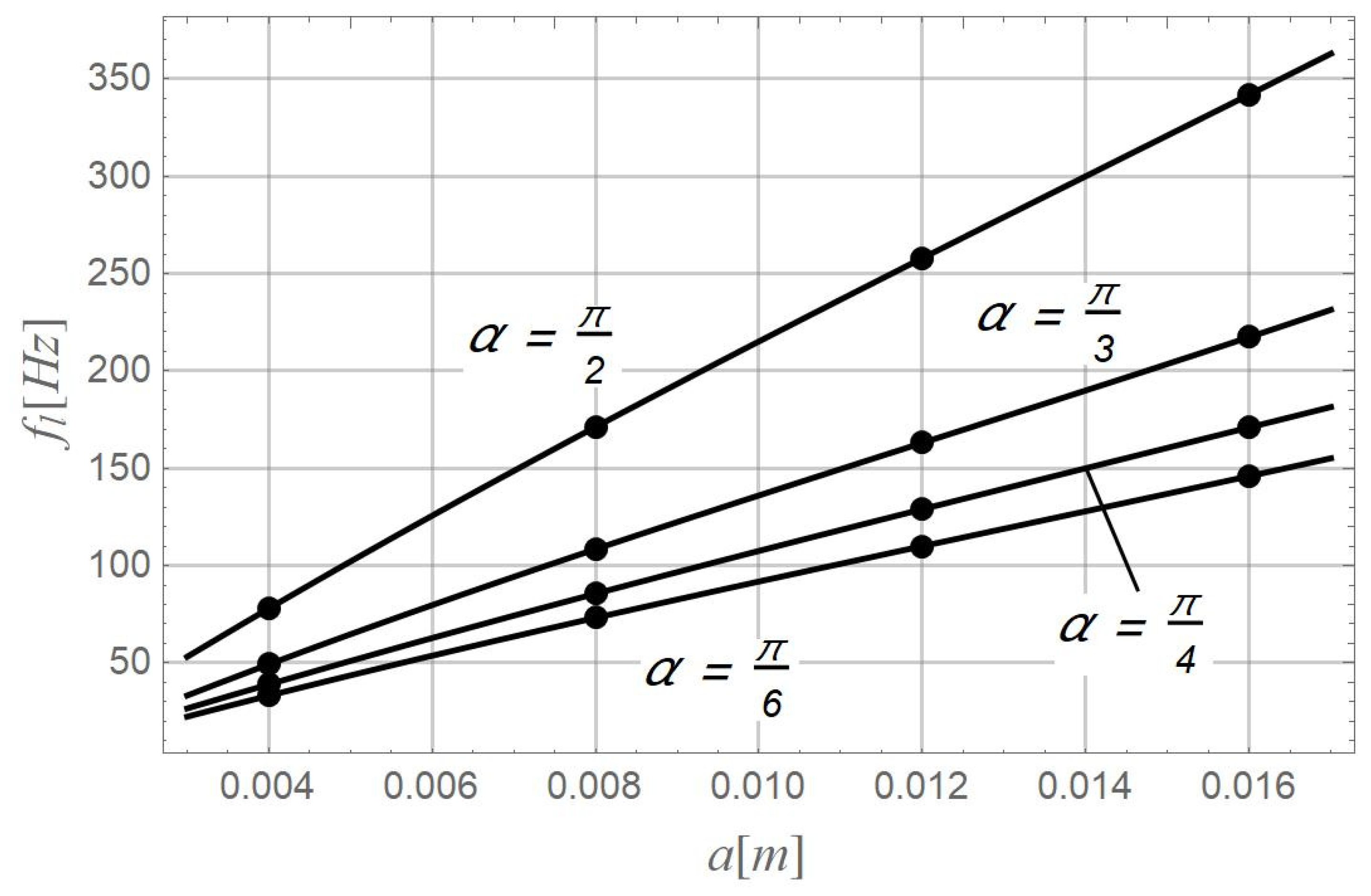
presents the computed periods T_l, obtained using formula (36), as well as the corresponding frequencies f_l = 1/T_l, for different values of the re-entrant angle α and various cross-sectional dimensions a. The unit mass ratio M/m = 1 is assumed. In Table 3, the angular frequency ω₀ is calculated according to Equation (28). Based on the values presented in Table 3, Figure 4 is constructed. The data in Table 3 and the corresponding $f_l-a$ diagrams in Figure 4 show that the vibration frequency increases with increasing cross-sectional dimension a, with a more pronounced effect at higher values of α. This behavior is attributed to the increase in structural stiffness, reflected in higher values of ${\omega }_0^2$. From Equation (38), it follows that the oscillation frequency is primarily governed by system stiffness and geometric parameters, while the amplitude depends on initial conditions and nonlinear effects.

By comparing the results in Table 3 and in Figure 4 with those given in Table 2 for identical re-entrant angles $\mathit{\alpha }$ and the same values of parameter a, it is concluded that a higher mass ratio M/m (see Table 2) in comparison to M/m = 1 (see Table 3) leads to a decrease in frequency. The conclusion is consistent with the theoretical analysis presented in Section 3.

Finally, it is concluded that all theoretical predictions strongly agree with those obtained experimentally.

4.4. Influence of Material Properties on Vibration Response

The influence of material properties on the vibration response is an important design consideration. As is known, the unit can be manufactured using 3D printing from different materials (e.g., PLA, TPU, etc.). These materials differ in their properties, particularly in specific density ρ and Young’s modulus E, compared to the steel used for the experimental model. For a unit with a square cross-section of 8 mm × 8 mm and an angle α = π/3, the predicted vibration frequency was calculated for structures made of PLA (ρ = 1250 kg/m³, E = 3 GPa) and TPU (ρ = 1250 kg/m³, E = 50 MPa). It was assumed that M/m = 1. The calculations were performed using Equation (32) and the initial angular velocity ${\dot{\phi }}_0$ = 1 rad/s. The obtained results are presented in

Table 4. Comparison of oscillation frequencies for units with identical dimensions made of different materials.

Material	$\mathit{\varrho } (\frac{\mathbf{k}\mathbf{g}}{{\mathbf{m}}^3})$	$\mathit{E} (\mathbf{P}\mathbf{a})$	${\mathit{\omega }}_0 (\frac{\mathbf{r}\mathbf{a}\mathbf{d}}{\mathbf{s}})$	${\mathit{T}}_{\mathit{l}} (\mathbf{s})$	${\mathit{f}}_{\mathit{l}} (\mathbf{H}\mathbf{z})$	${\mathit{\phi }}_{\mathit{m}\mathit{l}} (\mathbf{r}\mathbf{a}\mathbf{d})$
Fe	7850	2 1011	359.0	0.0092	108.5	0.0014
PLA	1250	3 109	34.80	0.0949	10.53	0.0152
TPU	1250	5 107	4.500	0.7351	1.360	0.1170

.

From Table 4, it can be seen that the frequency fₑ of the steel unit is significantly higher than that of the plastic materials, while the deformation and amplitude of vibration is much smaller. For applications requiring enhanced energy storage and large deformation capacity, it is preferable for the Young’s modulus E to be as low as possible (TPU is a flexible material), since larger deformations can then be achieved. The vibration frequency is lower for materials with a smaller Young’s modulus than for steel. The Young’s modulus of TPU is about 60 times lower than that of PLA, while the frequency decreases by approximately a factor of 8. TPU is a soft material suitable for low-frequency vibration application (around 1 Hz), whereas PLA is suitable for higher frequencies (around 10 Hz). However, the main drawback of this type of structure is the difficulty in maintaining structural stability and controlling its shape. Therefore, the use of soft filling materials is proposed as a strategy to achieve low-frequency response while maintaining structural stability.

Overall, the results demonstrate that the proposed analytical model provides accurate predictions of vibration characteristics and successfully captures the coupled effects of geometric nonlinearity, mass distribution, and material properties. The model is therefore suitable for design-oriented analysis of re-entrant structures.

5. Model of the Filled Structure

The comparison between empty and filled configurations is motivated by the need to control vibration characteristics through structural modification. While the empty unit provides a baseline dynamic response governed by geometry, the introduction of soft filling enables independent tuning of effective mass and stiffness, which is essential for achieving low-frequency response and controlled energy redistribution within the system. This choice of configuration is further justified by the need to isolate and quantify the individual contributions of geometry, inertia, and material properties to the overall dynamic response. The empty configuration represents a purely geometry-controlled system, while the filled configuration introduces additional mass and stiffness effects. This enables a systematic investigation of the coupled geometric–inertial–material interactions, providing a clear framework for evaluating the role of soft filling in modifying vibration characteristics.

The objective of this study is to design a unit cell that exhibits low-frequency vibrations with small amplitudes while maintaining structural stability. A key question is whether the filled unit can provide improved vibration performance in terms of frequency reduction and energy redistribution compared to the empty structure. In this section, the dynamic behavior of the filled unit is analyzed.

The filling material is modeled as a linear elastic element characterized by stiffness k_f, which represents an idealized constitutive assumption. This simplification is adopted to capture the primary effect of the filling on the global dynamic response while maintaining analytical tractability of the model. The formulation is valid under the assumption of small deformations and linear elastic behavior of the filling material. In practical applications, such as polymer foams or viscoelastic materials, the constitutive response may exhibit rate dependence, damping effects, and nonlinear behavior. These effects are not explicitly included in the present model and therefore represent a limitation of the current approach. Nevertheless, the adopted approximation provides a physically consistent first-order description of the coupling between inertia and stiffness effects, and serves as a basis for further extensions involving more complex constitutive laws.

A filling material with stiffness k_f and mass m_f is introduced into the unit cell. The presence of the filling modifies the kinetic energy of the system through its inertial contribution. Accordingly, the kinetic energy includes an additional term given by

$$T_f={\displaystyle \frac{1}{2}}{m}_f{l}^2{\dot{\phi }}^{2}co{s}^2(\mathit{\alpha }+\phi )$$

(40)

The mass of the filler is determined from the geometry of the internal cavity of the hexagonal unit cell. The cavity area is obtained as twice the area of an isosceles trapezoid with bases L and (L − 2lcosα) and height lsinα, yielding $A=2\left(L-lcos\mathit{\alpha }\right)lsin\mathit{\alpha }$. Accordingly, the filler mass is given by $m_f=2{\rho }_{f}a\left(L-lcos\mathit{\alpha }\right)lsin\mathit{\alpha }$ where ${\rho }_f$ is the density of the filling material, and a is the thickness of the filling. Here, α denotes the initial geometric angle of the unit cell, and therefore the filler mass $m_f$ is constant during motion.

The potential energy of the filling is

$$V_{fg}=m_{f}gl(sin \left(\mathit{\alpha }+\phi \right)-sin\mathit{\alpha })$$

(41)

Due to the elastic properties of the filling it is

$$V_{fk}={\displaystyle \frac{1}{2}}{k}_f{l}^2{\left(sin\left(\mathit{\alpha }+\phi -{\phi }_n\right)\right)}^2$$

(42)

Extending the total kinetic energy (9) with (40), and the potential energy (19) with (41) and (42), the equation of motion (22) is transformed into

$$\begin{array}{cc}\hfill [{\displaystyle \frac{10}{3}}+2\mathit{cos}2(\mathit{\alpha }& +\phi )+{\displaystyle \frac{4M+m_f}{2m}}(1+\mathit{cos}(2(\mathit{\alpha }+\phi )))]\ddot{\phi }-{\displaystyle \frac{4M+4m+m_f}{2m}}\mathit{sin}\left(2\left(\mathit{\alpha }+\phi \right) \right){\dot{ \phi }}^2\hfill \\ & +12{\omega }_0^2\left(-{\phi }_n+\phi \right)+{\displaystyle \frac{cos\left(\mathit{\alpha }+\phi \right)}{m}}[\left(2M+4m+m_f\right){\omega }_1^2-k_f\mathit{sin}(2(\mathit{\alpha }+{\phi }_n))]\hfill \\ & +{\displaystyle \frac{k_f}{2m}}\mathit{sin}(2\left(\mathit{\alpha }+\phi \right))=0\hfill \end{array}$$

(43)

where the value ${\phi }_n$ corresponds to the case when $\phi =0$ and satisfies the relation

$$-12{\omega }_0^2{\phi }_n+{\displaystyle \frac{cos\left(\mathit{\alpha }\right)}{m}}[\left(2M+4m+m_f\right){\omega }_1^2-k_f\mathit{sin}(2(\mathit{\alpha }+{\phi }_n))]+{\displaystyle \frac{k_f}{2m}}\mathit{sin}(2\mathit{\alpha })=0$$

(44)

The Equation (43) and the expression (44) are strongly nonlinear. For the case of small vibrations in the horizontal plane the Equations (43) and (44) are simplified and the period of vibration is

$$T_f=2\pi \sqrt{{\displaystyle \frac{\frac{5}{3}+\frac{M}{m}+\frac{m_f}{4m}+\left(\frac{M}{m}+\frac{m_f}{4m}+1\right)cos(2\mathit{\alpha })}{6{\omega }_0^2+\frac{k_f}{2m}cos(2\mathit{\alpha })}}}$$

(45)

The period of vibration depends not only on the mass ratio M/m, structural stiffness, and re-entrant angle α, but also on the mass and stiffness of the filling material..

5.1. Analysis of Vibration Characteristics of the Filled Unit

The frequency of vibration of the unit with filling (41) has the form $f_f\approx \sqrt{k_{eff}/m_{eff}}$ where the effective stiffness $k_{eff}$ depends on the stiffness of the filling $k_f$ and the effective mass $m_{eff}$ on the filling mass $m_f$. Two cases are possible:

(1)

If $m_{eff}$ is the dominant parameter, the frequency of the filled unit is lower than the frequency of the empty unit. This corresponds to an inertia-dominated regime.

(2)

If $k_{eff}$ is dominant, the frequency of vibration of the filled unit is higher than that of the empty unit. Increasing the stiffness of the filling the frequency of vibration is also increasing. This regime is stiffness-dominated.

• Case 1. Inertia-dominated regime (dominant ${\mathit{m}}_{\mathit{f}},$ weak influence of ${\mathit{k}}_{\mathit{f}}$)

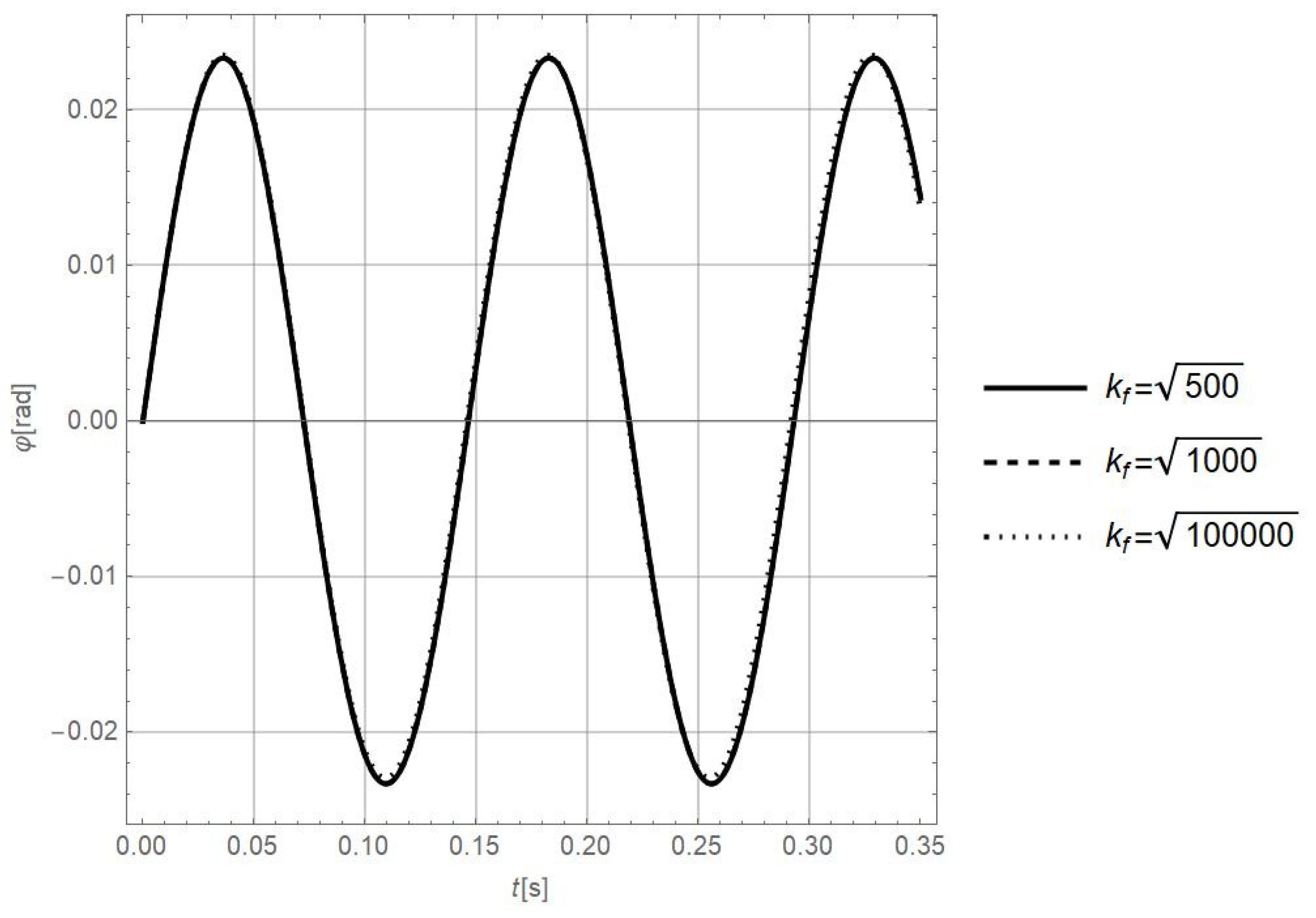
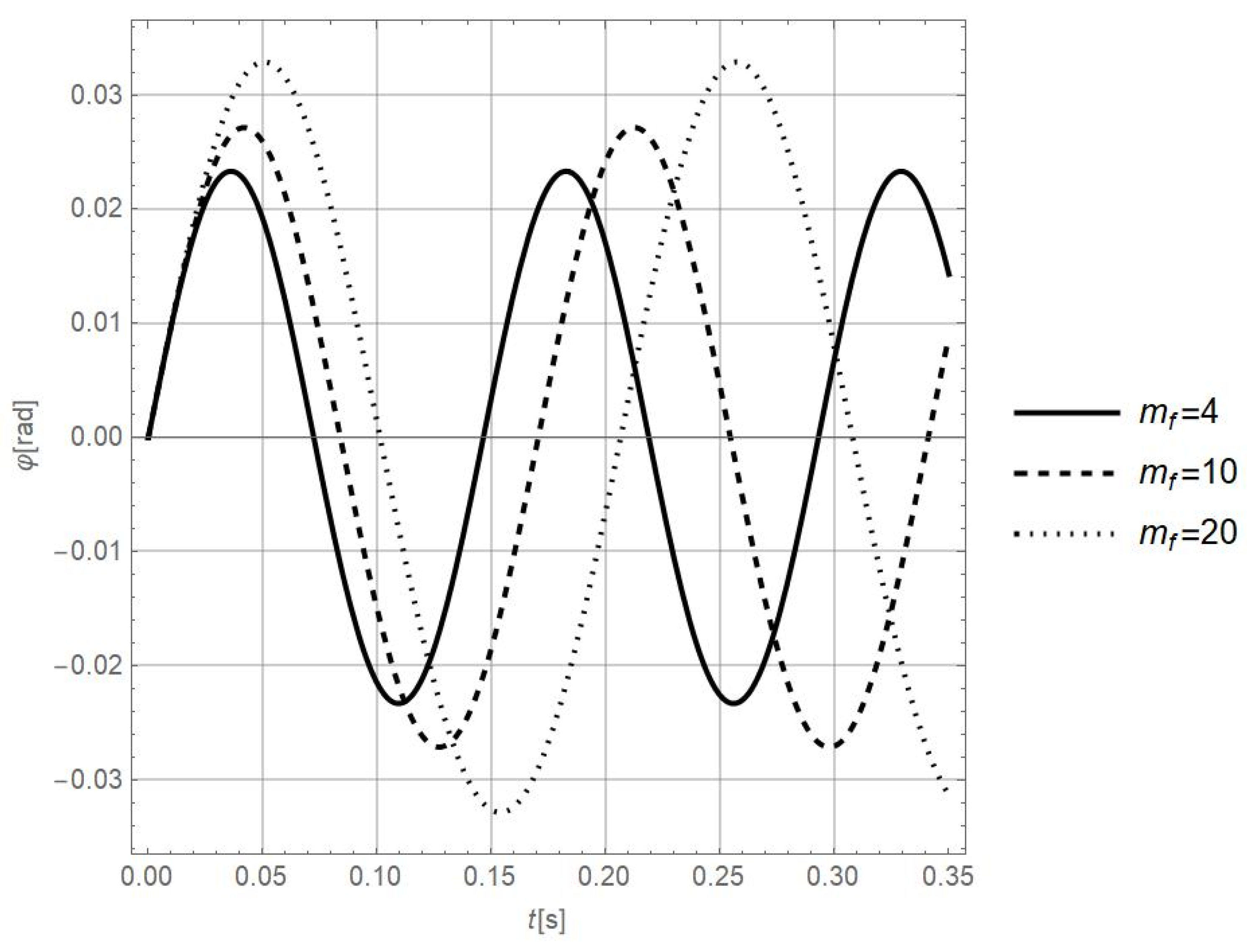
In Figure 5 the solution of the Equation (39) with (40), i.e., φ (t) diagrams for various filling masses m_f, are plotted. The parameters are M = 2, m = 1, ${\omega }_0^2=1500$, ${\omega }_1^2=100$, $k_f=1000, \mathit{\alpha }={\displaystyle \frac{\pi }{3}}$, with initial conditions $\phi (0)=0$ and $\dot{\phi }\left(0\right)=1.$ It is observed that both the amplitude and the oscillation period increase with increasing $m_f$. For these parameter values the obtained results are in good agreement with the analytical expression (41), which shows that larger_$m_f$ leads to longer periods and higher amplitudes of vibration.

For these parameter values the $\phi (t)$ diagrams for various filling stiffness $k_f$ are presented in Figure 6. The unit parameters are M = 2, m = 1, ${\omega }_0^2=1500$, ${\omega }_1^2=100$, $m_f=4,$ with initial conditions $\phi (0)=0$ and $\dot{\phi }\left(0\right)=1.$ The values considered are $k_f=\sqrt{500}; \sqrt{1000}; \sqrt{100000}.$

Comparing Figure 5 and Figure 6 it is observed that in contrast to the stiffness parameter of the filling k_f, the filling mass m_f has a more significant effect on the vibration frequency. The period of vibration increases with higher filling mass and lower stiffness, as also evident from (45). These results indicate that the filling mass has a more pronounced influence on vibration characteristics than the filling stiffness. Therefore, for design purposes, the structural frame should remain sufficiently stiff to ensure stability, while the filling should be soft and relatively dense to enhance inertial effects.

In Figure 7, the solution $\phi (t)$ of Equation (43) with (44) for different values of the re-entrant angle is plotted. The results show that, in the filled unit, both, the amplitude of vibration and the period increases as the angle decreases. This statement is in agreement with that for the empty unit.

If the filling mass m_f has a more pronounced influence on the oscillation frequency than the filling stiffness k_f, this indicates that the addition of filling primarily contributes to the increase in inertia rather than to the structural stiffness. In such a configuration, the filling material can be characterized as relatively heavy and compliant, providing negligible stiffness compared to the re-entrant frame. Consequently, the external re-entrant structure acts as the main load-bearing component, while the filling behaves as an inertial addition. This type of system typically corresponds to a stiff outer framework combined with a soft, low-stiffness filling material, such as a viscoelastic or foam-like medium, leading to a reduction in the natural frequency.

• Case 2. Stiffness-dominated regime (${\mathit{k}}_{\mathit{f}}$ is dominant and the effect of ${\mathit{m}}_{\mathit{f}}$ is small)

Let us consider the re-entrant unit made of PLA, a stiff structural material to ensure load-bearing capacity and geometric stability, and with TPU, a soft filling material to enhance energy dissipation. Density and Young’s modulus of elasticity for both materials and dimensions of the already-studied steel model are given in Section 4.

For this model the stiffness of the filling k_f is sufficiently large and the dynamic response of the unit cell is governed primarily by the effective stiffness rather than by inertia. From Equation (45), it follows that the period of vibration is inversely proportional to the square root of the effective stiffness term in the denominator. As k_f increases, this term grows, leading to a decrease in the period of oscillation. In this stiffness-dominated regime, the contribution of the filling significantly enhances the overall rigidity of the system. Consequently, the filled unit exhibits a shorter period (i.e., higher frequency) compared to the empty unit. This behavior is consistent with the classical statement that the increase in effective stiffness outweighs the effect of the added mass. 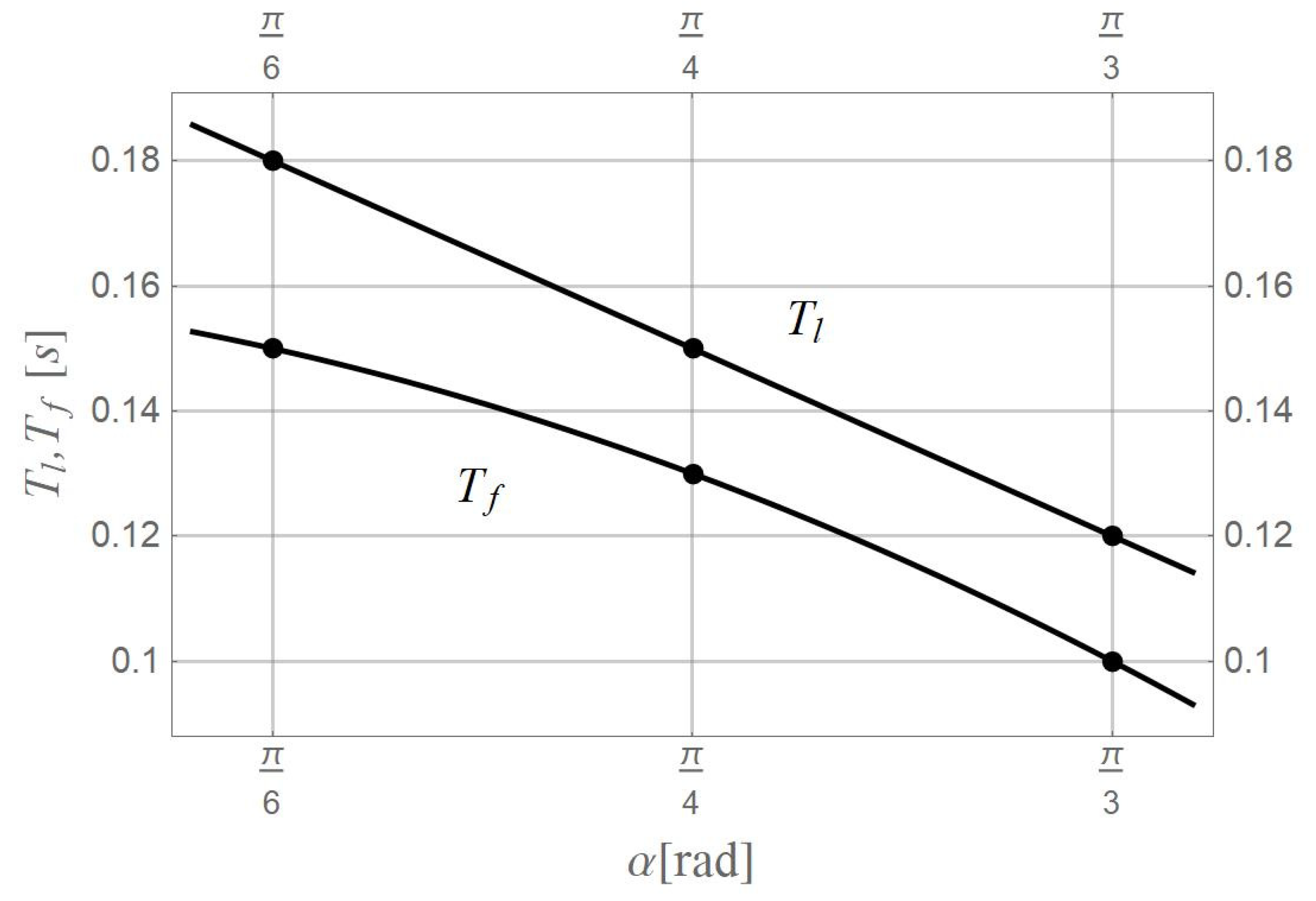This trend is clearly observed in Figure 8, where the period of vibration of the filled unit lies below that of the empty unit for the same values of the re-entrant angle. The results indicate that the vibration frequency of the filled unit may remain relatively high, which represents a limitation of the configuration.

In addition, comparing the diagrams in Figure 8, for the empty ($T_l$) and filled ($T_f$) units, it is evident that the re-entrant angle itself acts as a parameter that reduces the period of vibration in both types of units.

The results indicate that the vibration frequency remains relatively high for the filled unit, which represents a limitation of the model. A practical approach to reduce the frequency is to adjust the degree of filling η.

5.2. Influence of the Filling Degree on Vibration Frequency

The degree of filling $\eta$ can vary from 0 (empty structure) to 1 (fully filled structure). Taking $\eta$ into account, the vibration frequency $f_f=1/T_f$, according to (45), is expressed as

$$f_f=({\displaystyle \frac{1}{2\pi }})\sqrt{{\displaystyle \frac{A+B\eta \mathrm{c}\mathrm{o}\mathrm{s}(2\mathit{\alpha })}{8/3+C\eta +\left(2+C\eta \right)cos(2\mathit{\alpha })}}}$$

(46)

where $A={\displaystyle \frac{3E{a}^2}{\rho l^3}}$ is the coefficient of the structure stiffness, $B={\displaystyle \frac{E_{f}a{L}^3}{8H\rho {la}^2}}$ is the coefficient of the filling stiffness, $C={\displaystyle \frac{m_f}{4m}}={\displaystyle \frac{{\rho }_{f}tHa}{4\rho {la}^2}}$ is the mass ratio of filling to the beam, $t=2\left(L-lcos\mathit{\alpha }\right), H=2lsin\mathit{\alpha }$, and L is the unit width. It is obtained that the vibration frequency f_f (42) depends on the filling parameter $\eta :$ for higher values of $\eta ,$ the unit becomes stiffer, as the increase in filling stiffness dominates over the added mass. The frequency tends to zero if $\eta =A/B$.

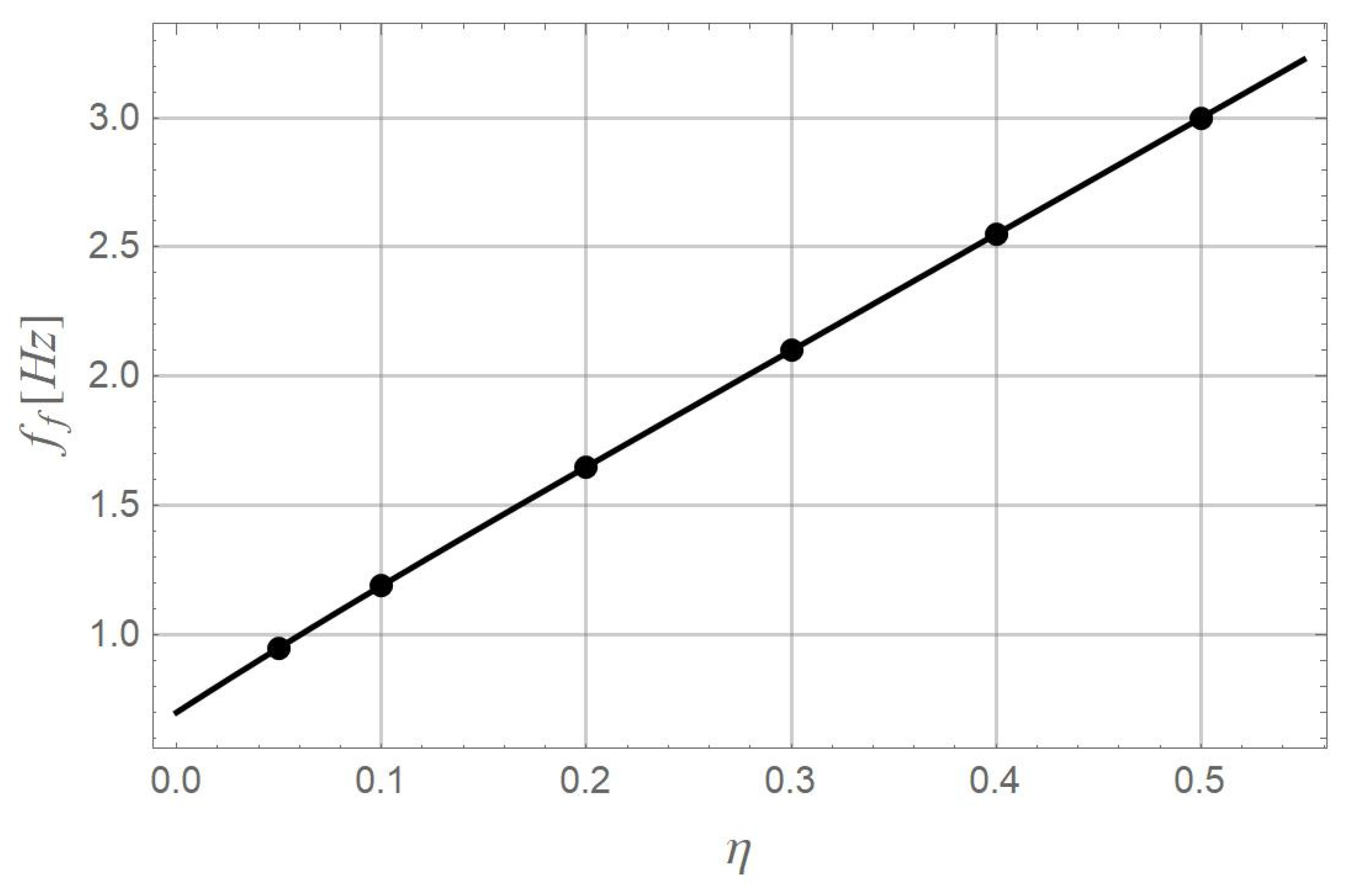
The frequency given by the Equation (42) is computed for different values of $\eta$ and parameters α =$\pi /3$, E = 3 × 10⁹ Pa, E_f = 5 × 10⁷ Pa, ρ = ρ_f = 1250 kg/m³, a = 0.008 m, and ω₀ = 359 s⁻¹, and is plotted in Figure 9. The obtained diagram shows that reducing η leads to lower vibration frequencies. Namely, the decreasing of the filling degree η leads to decrease of the effective stiffness (η$E_{f,}$).

Finally, to achieve low-frequency vibrations (1–2 Hz), it is recommended to use a low filling degree η = 0.05–0.15, combined with a soft filling material such as TPU in an open-cell configuration (e.g., gyroid). This approach enables a reduction in effective stiffness while preserving sufficient structural integrity, thereby facilitating low-frequency response.

6. Conclusions

It can be concluded that:

• The filled re-entrant hexagonal unit introduced in this paper can be effectively utilized for vibration control, particularly in the low-frequency range. A proper design that captures the coupled geometric–inertial effects enables efficient vibration attenuation and favorable energy redistribution within the system. The oscillation parameters obtained through the analytical procedure developed in this study show excellent agreement with numerical results and good correlation with available experimental data.
• The vibration response of the filled re-entrant unit is rigorously governed by the ratio of effective stiffness to effective mass, leading to two fundamentally distinct regimes of behavior: inertia-dominated and stiffness-dominated behavior.
• In the inertia-dominated regime, the addition of filling unambiguously reduces the natural frequency while simultaneously increasing both the oscillation period and amplitude, thereby establishing mass as the governing parameter. The influence of the filling stiffness is secondary in this regime, confirming that mass effects dominate over stiffness effects in practical soft-filling configurations. Physically, this regime corresponds to a stiff load-bearing re-entrant frame combined with a soft, compliant, and relatively heavy filling, where the filling primarily acts as an inertial contribution. This configuration is particularly suitable for low-frequency vibration control.
• In contrast, in the stiffness-dominated regime, when the filling stiffness is dominant, the behavior is reversed: the filled unit exhibits higher frequencies and shorter periods than the empty one. In this case, the filling contributes primarily to stiffness, reducing both amplitude and period. However, the parametric dependence introduced through the filling degree η provides a direct and efficient tuning mechanism. It is obtained that a decrease in the filling degree reduces the effective stiffness, and thus lowers the vibration frequency. For practical designs, low filling degrees (η ≈ 0.05–0.15) are required to reach low-frequency ranges (1–2 Hz).
• The re-entrant angle is a key geometric control parameter in both regimes. In the filled system, its effect is strongly coupled with the properties of the filling material. A decrease in the re-entrant angle consistently leads to an increase in both the oscillation period and amplitude, highlighting its role in enhancing vibration response and energy redistribution.

The results indicate that optimal vibration performance is achieved with a low re-entrant angle, high filling mass, and low filling stiffness. The structural stiffness should remain sufficiently high to preserve geometric stability, while the filling should be soft and dense, enabling effective energy redistribution and a low-frequency response. The present model is based on a linear elastic approximation of the filling material, which ensures analytical tractability while capturing the dominant physical effects. However, extensions to include viscoelastic, damping, and rate-dependent behavior of the filling material are left for future research directions.