Article

Multi-Scale Fractional-Order Image Fusion Algorithm Based on Polarization Spectral Images

Navigation College, Dalian Maritime University, Dalian 116026, China
*
Author to whom correspondence should be addressed.
Appl. Sci. 2026, 16(9), 4087; https://doi.org/10.3390/app16094087
Submission received: 19 March 2026 / Revised: 14 April 2026 / Accepted: 16 April 2026 / Published: 22 April 2026

Abstract

With the continuous advancement of polarization spectral sensing technology, multi-band polarization image fusion has emerged as a novel approach to image fusion. By integrating spectral and polarization information, this method overcomes the limitations of relying on a single information source and significantly improves overall image quality. To address this, this paper proposes a new polarization spectral fusion algorithm. First, feature matching is employed to achieve pixel-level spatial alignment of multi-band polarization images. Then, a fusion strategy based on multi-scale decomposition and singular value decomposition is adopted to preserve structural information and fine details. Subsequently, fractional-order processing and guided filtering are applied to enhance details and suppress noise. Finally, a progressive reconstruction from low to high scales is performed to ensure hierarchical consistency and information integrity throughout the fusion process. In addition, spectral information is utilized for color restoration, enabling the final image to achieve high spatial resolution while maintaining natural and rich color representation.Experimental results demonstrate that the proposed method effectively integrates features from different spectral bands and polarization information while preserving maximum similarity, leading to significant improvements in both image quality and detail representation.

1. Introduction

In the field of target detection and recognition, the current challenges are compounded by complex and changing environments. Under conditions involving concealed targets amidst backgrounds, weak radiation objects, and strong interference backgrounds, traditional methods relying on light intensity, spatial, or single-spectral information often prove ineffective for discrimination. Consequently, applications in areas such as military reconnaissance, environmental monitoring, and precision agriculture face limitations [1,2]. Polarization spectral imaging extends traditional three-dimensional information to seven dimensions, simultaneously capturing multi-dimensional data including intensity, polarization, spectral characteristics, and spatial information of the target. This technology enables precise description of surface roughness, material composition, and other attributes across different wavelengths, revealing various aspects of the target’s inherent state, thereby paving a new way to overcome the bottlenecks of conventional optical imaging techniques [3,4]. The rapid advancement of photoelectric detection devices and signal processing methods has significantly enhanced the ability to extract and fuse polarization spectral information from targets, making this a current hotspot in optical imaging research [5,6].
High-quality acquisition of target polarization spectral images is a prerequisite for effective fusion and precise identification, with the core challenge being the collaborative modulation of polarization-spectral information. Existing research methods include Acousto-Optic Tunable Filters (AOTF), Liquid Crystal Tunable Filters (LCTF), and integrated detectors [7,8,9]. The U.S. Army Research Laboratory (ARL) developed a polarization spectral imaging system utilizing AOTF and Liquid Crystal Variable Retarders (LCVR), operating within the 0.4–11.5 µm range. This system employs electronic control technology to enhance imaging timeliness, but suffers from a low signal-to-noise ratio due to the influence of acousto-optic sensor noise [10]. Domestically, Lu Fang from Xidian University adopted the Polarization-Difference Channel Imaging Spectropolarimetry (PDCISP) technique, achieving simultaneous acquisition of three orthogonal polarization modulation modes. This expands the effective optical path difference range and effectively suppresses inter-channel crosstalk [11]. The team led by Zhang Fei from the Chinese Academy of Sciences proposed a novel configurable dual-mode detection method, integrating it with a miniaturized shared-aperture meta-optical system. This enables simultaneous operation in the 8–14 µm band with a large 70-degree field of view, facilitating multi-mode, multi-target detection and laying the foundation for the miniaturization and practical application of multifunctional optical systems [12]. The compressed full-Stokes hyperspectral imaging technique proposed by Fan et al. employs a combined modulation of quarter-wave plate, linear polarizer, and LCTF, coupled with numerical reconstruction algorithms. This reduces reconstruction time by 83.73%, ultimately achieving high-precision and rapid calculation of Stokes parameters [13]. However, current technology still faces challenges such as the difficulty in balancing broadband operation with high resolution, imaging lag in dynamic scenes, and low integration levels, making it difficult to meet the demands of mobile and real-time detection.
Polarization-spectral image fusion is a method for complementary advantages of multi-source information. It effectively enhances target contours, reduces background noise, and improves image discriminability, serving as a crucial step connecting data acquisition and object recognition [14,15,16,17]. Early fusion techniques primarily employed multi-scale transforms such as wavelet transform and non-subsampled contourlet transform, as well as sparse representation. Zhu Pan et al. proposed a novel fusion algorithm based on Dual-Tree Complex Wavelet Transform (DTCWT) and sparse representation, which balances the fusion of infrared polarization and intensity images while preserving details and eliminating noise [18]. Building on this foundation, some research has proposed a hyperspectral image color space transformation method based on color space mapping, which accurately fuses spectral information from specular reflection with polarization information from diffuse reflection, providing an effective technical approach for applications such as astronomical observation [19]; Consequently, this project plans to employ a weighting method based on regional energy and Local Binary Pattern (LBP) operators to jointly analyze fused feature images, spectral images, and polarization images, thereby improving the information completeness and robustness of the images [20]. Furthermore, a method combining principal component analysis and energy weighting can effectively fuse multi-dimensional features to enhance the detail and edge characteristics of objects [21]; On this basis, research has been conducted on an edge detail enhancement algorithm based on rolling guidance filter and sparse representation. First, bilateral filtering is applied to the Stokes parameter images within the polarization vector space to suppress noise while preserving polarization characteristics. Second, RGF is used to decompose the grayscale and low-noise polarization images into a base layer and a detail layer. Employing a multi-scale fusion strategy ultimately achieves a synergistic improvement in visual quality and brightness while maintaining complex details [22].
In recent years, with the advancement of deep learning, various deep fusion models have emerged. Generative Adversarial Networks (GANs) represent an approach that utilizes polarization hyperspectral data for deep feature extraction and weight fusion [23]; By efficiently utilizing Degree of Linear Polarization (DoLP) images, an encoder-decoder based dense convolutional network demonstrates strong fusion performance across three dimensions: grayscale, edge, and texture [24]; This research innovatively combines multi-dimensional self-attention (F-MSA) with entropy-based fusion techniques, playing a significant role in the fusion process and exhibiting high adaptability to multi-modal tasks such as complex environment monitoring and visible light fusion [25]. Furthermore, an unsupervised deep neural network, employing a customized framework and loss function, fuses polarization images without relying on ground-truth image information to enhance visual quality and quantitative metrics [26]; Based on the Non-subsampled Contourlet Transform (NSCT) and Convolutional Neural Networks (CNN), denoising and polarization parameters are fused to obtain polarization feature maps. Techniques including NSCT decomposition, feature extraction and normalization, block-based strategies for determining fusion coefficients, and inverse transform reconstruction are utilized, thereby improving target detection accuracy in polarization images [27]; Leveraging a semantic-guided dual-discriminator generative adversarial network (SGPF-GAN), the fusion process is guided by block-weighted Polarization Image Quality Discriminators (PIQD). By establishing an adversarial game between the generator and the two discriminators, the detection and segmentation performance for transparent and camouflaged concealed targets can be significantly enhanced [28].
Although research on multi-band polarization image fusion has begun, effective fusion algorithms remain scarce. This is primarily due to two reasons: first, traditional polarization spectrum acquisition devices feature complex structures and large volumes; second, conventional data fusion methods employ a relatively single fusion strategy when processing polarization spectrum information, leading to information loss during the fusion process. To address these issues, this paper constructs a time-division polarization spectrum system for multi-band polarization image data acquisition. Image feature matching is employed to achieve pixel-level spatial alignment, ensuring data consistency throughout the subsequent fusion process. Through a multi-scale decomposition and SVD-based fusion strategy, the intensity information and polarization information from different bands are respectively fused into novel Gaussian pyramids and Laplacian pyramids that encompass features from all bands. Fractional-order processing and guided filtering techniques not only eliminate noise components from the polarization information but also enhance texture details. Finally, a progressive recovery and weighted fusion rule from low scale to high scale is proposed, eliminating information loss caused by single fusion rules. Color rendering based on original spectral information ensures that the final high-resolution fused images simultaneously possess authentic and rich colors.
Compared with previous work, the main contributions of our proposed method are as follows:
1.
A time-division polarization spectrum system is proposed, which can acquire polarization spectrum images across different bands while ensuring spatial resolution. Through feature matching techniques, pixel-level spatial alignment of polarization images from different bands is guaranteed.
2.
Based on multi-scale decomposition and SVD, the spectral information and polarization information from different bands are fused at various scales, maximizing the retention of feature information from each band. By integrating fractional-order processing and guided filtering, noise components in the polarization information are eliminated while texture details are enhanced.
3.
Through a progressive recovery and weighted fusion strategy from low scale to high scale, information loss caused by single fusion rules is eliminated, ensuring the imaging quality and natural appearance of the fused images.
The remainder of this paper is organized as follows: Section 2 introduces fundamental concepts, including SVD, Stokes vectors, and fractional-order differentiation, and elaborates on the fusion rules proposed in this paper. Section 3 discusses the experimental validation of the theoretical model and presents the corresponding results. Section 4 presents subjective and objective analyses comparing our method with other fusion algorithms. Section 5 concludes the paper and discusses its limitations.

2. Correlation Theory

2.1. Singular Value Decomposition

Singular Value Decomposition (SVD) is an important matrix factorization method in linear algebra, used to decompose any matrix into the product of three simpler matrices. This method is applicable not only to square matrices but also to rectangular matrices of any shape, serving as a generalization of eigenvalue decomposition to non-square matrices. SVD decomposes a matrix into an orthogonal matrix, a diagonal matrix, and the transpose (or conjugate transpose) of another orthogonal matrix, where the diagonal elements of the diagonal matrix are called singular values.
For an m × n real matrix, its singular value decomposition can be expressed as:
A = U Σ V
Here, U is an m × m orthogonal matrix satisfying U U = I , and its column vectors are called left singular vectors. v is an n × n orthogonal matrix satisfying V V = I , and its column vectors are called right singular vectors. ∑ is an m × n rectangular diagonal matrix whose diagonal elements are the singular values of matrix A. These singular values are typically arranged in descending order, while all off-diagonal elements are zero.
SVD has a wide range of applications in mathematics and engineering, including data dimensionality reduction and Principal Component Analysis (PCA), recommendation systems, image compression and denoising, and solving linear equations. Its core idea is to achieve a low-rank approximation of the original data by retaining the largest singular values and their corresponding singular vectors, thereby removing noise and extracting key features. SVD reveals the geometric essence of a matrix in linear transformations, namely the process of “rotation-stretching-rotation,” and provides complete information about the four fundamental subspaces of a matrix (column space, row space, null space, and left null space).
In the context of images, an image can be represented as a large matrix, where each element corresponds to a pixel value. Through SVD decomposition, the image can be expressed as a sum of rank-1 matrices (outer product terms). Since singular values typically decay exponentially, retaining only the largest singular values along with their corresponding singular vectors allows for reconstructing a visually high-quality image using minimal storage space, enabling efficient compression. Additionally, smaller singular values often correspond to high-frequency noise in the image; setting them to zero can achieve image denoising while preserving the main structure of the image.

2.2. Stokes Vector

The polarization of light can be described by several methods, including the electric field vector method, the Jones matrix method, the Poincaré sphere, and the Stokes vector method. In practical applications of polarization imaging, the most common approach is to obtain the required polarization characteristic parameters by acquiring the Stokes vector. Therefore, this paper focuses on the Stokes vector representation of polarized light.
In 1852, Stokes proposed using four parameters to describe the intensity and polarization state of light waves. Unlike the Jones vector, the Stokes vector can describe fully polarized light, partially polarized light, and completely unpolarized light, as well as both monochromatic and non-monochromatic light. These four Stokes parameters are time-averaged values of light intensity (averaged over a time interval sufficiently long for measurement) and together form a four-dimensional mathematical vector. They are defined as follows:
S 0 = E x 2 + E y 2 S 1 = E x 2 E y 2 S 2 = 2 E x E y cos δ S 3 = 2 E x E y sin δ
In the Equation, S 0 represents the total intensity of light waves, which is always non-negative. S 1 denotes the difference between the horizontal and vertical linear polarization components, describing the preferential polarization degree of light in the 0° and 90° directions. S 2 represents the difference in intensity between the 45° and 135° linear polarization components, describing the preferential polarization degree of light in the ±45° directions. S 3 represents the difference in intensity between the right-handed circular polarization and left-handed circular polarization components, describing the degree of circular polarization of light. S 3 > 0 indicates that right-handed circular polarization is dominant, while S 3 < 0 indicates that left-handed circular polarization is dominant. In practical applications, Stokes can also be directly represented by image intensity [29,30,31]:
S 0 = I ( 0 ) + I ( 90 ) S 1 = I ( 0 ) I ( 90 ) S 2 = I ( 45 ) I ( 135 ) S 3 = I ( R ) I ( L )
In the Equation (3), I ( 0 ) , I ( 45 ) , I ( 90 ) , and I ( 135 ) represent the four polarization images obtained by the sensor at directions of 0°, 45°, 90°, and 145°, respectively. I ( R ) denotes the right-handed circular polarization image, and I ( L ) denotes the left-handed circular polarization image. Typically, to combat noise interference, the value of S 0 is taken as half the sum of the four angles. In addition, in natural environments, the linear polarization component predominantly dominates the polarized light. In contrast, the intensity of the circular polarization component (i.e., Stokes parameter S 3 is typically only on the order of 10 4 to 10 3 of the total light intensity, significantly smaller than the linear polarization component. Therefore, from the perspective of energy contribution, the polarized light in nature can be considered dominated by linear polarization, with elliptically polarized light merely manifesting as a minor and negligible correction term. Based on this prior understanding, the S 3 component will not be considered in the subsequent analysis of this paper, simplifying the Stokes vector to the following form:
S 0 = I ( 0 ) + I ( 45 ) + I ( 90 ) + I ( 135 ) / 2 S 1 = I ( 0 ) I ( 90 ) S 2 = I ( 45 ) I ( 135 )
According to Malus’s theorem, the light intensity values for different polarization directions are given by Equation (5).
I 0 = 1 2 S ( 1 p ) + S p cos 2 ( θ 0 ° ) I 45 = 1 2 S ( 1 p ) + S p cos 2 ( θ 45 ° ) I 90 = 1 2 S ( 1 p ) + S p cos 2 ( θ 90 ° ) I 135 = 1 2 S ( 1 p ) + S p cos 2 ( θ 135 ° )
Here, p is the degree of polarization (DOP) and θ is the angle of polarization (AOP). Using Malus’s theorem and the Stokes vector, the degree of polarization and polarization angle in the detected light can be determined, as shown in Equations (6) and (7).
p = S 1 2 + S 2 2 S ( 0 < p < 1 )
The value range of the degree of polarization is [0, 1]. The larger the value, the greater the proportion of fully polarized light. When DOP = 1, the light wave is fully polarized light; when DOP = 0, the light wave is natural light (completely non-polarized light); in other cases, the light wave is partially polarized light.
θ = 1 2 arctan S 2 S 1 ( S 2 > 0 , S 1 > 0 ) θ 0 , π 4 ( S 2 > 0 , S 1 < 0 ) θ π 4 , π 2 ( S 2 < 0 , S 1 < 0 ) θ π 2 , 3 π 4 ( S 2 < 0 , S 1 > 0 ) θ 3 π 4 , π
From the definition, it can be seen that the range of values for the polarization angle is [0, π ]. It should be noted that when performing actual calculations, the relative sizes of S 2 and S 1 , as well as the quadrant range, must be considered. Otherwise, calculation errors may occur. The calculation formula for AOP can also be expressed as:

2.3. GL Fractional Order Differential

Fractional-order differentiation is a mathematical theory that extends the order of differentiation from integers to arbitrary real numbers or even complex numbers. In contrast to the limitation of traditional differential equations, which can only describe instantaneous changes, fractional-order differentiation possesses long-term memory and the ability to model complex processes with historical dependence. Currently, with the significant development of fractional-order differentiation theory, there are typically three definitions. The first is the Grünwald–Letnikov (GL) definition, which is best suited for numerical computation and discrete implementation. The second is the Riemann–Liouville (RL) definition, which is often used for theoretical derivations. The third is the Caputo definition, which is commonly applied in engineering and control systems. Given that images are in discrete form, this paper focuses on explaining the GL definition.
f ( t ) = lim h 0 f ( t ) f ( t h ) h
Furthermore, according to the theory of integer-order derivatives, the second-order derivative of a function can be derived as follows:
f ( t ) = lim h 0 f ( t ) 2 f ( t h ) + f ( t 2 h ) h 2
By analogy, the definition of the nth-order derivative is obtained as follows:
f ( n ) ( t ) = lim h 0 r = 0 n ( 1 ) r n r f ( t r h ) h n
where r is an integer ranging from 0 to n, and n r = n ! r ! ( n r ) ! represents the standard binomial coefficient. By extending the integer n to any real number a (where a > 0 ), the following formula can be obtained:
f ( a ) ( t ) = lim h 0 r = 0 [ t a h ] ( 1 ) r a r f ( t r h ) h a
[ t a h ] represents the greatest integer not exceeding t a h , which ensures that only the interval from the starting point a to the current point t is covered. Then, we introduce the Gamma function to transform the binomial coefficient, originally representing integers, into a generalized binomial coefficient capable of representing fractions.
a r = Γ ( a + 1 ) Γ ( r + 1 ) Γ ( a r + 1 )
Finally, the Grünwald-Letnikov fractional-order derivative formula is obtained.
D a f ( t ) = 1 h a lim h 0 r = 0 [ t a h ] ( 1 ) r Γ ( a + 1 ) Γ ( r + 1 ) Γ ( a r + 1 ) f ( t r h )
Since we are dealing with discretization operations based on images, in image processing, h = 1 , and the formula is simplified to
D a f ( t ) = r = 0 N ( 1 ) r Γ ( a + 1 ) Γ ( r + 1 ) Γ ( a r + 1 ) f ( t r )
N represents [ t a h ] , which also indicates that fractional-order derivatives require memory of the historical context, rather than only observing the current changes. In contrast to integer-order derivatives, which can only enhance edges but lead to the loss of weak textures, fractional-order derivatives enable both the enhancement of details and the preservation of textures. This lays a theoretical foundation for our subsequent image processing tasks.

2.4. Multi-Scale Fractional-Order Enhanced Fusion Model

In related image fusion algorithms, a fixed, single rule is typically employed for fusion, which results in insufficient clarity of image edges and texture details after processing. This issue is particularly pronounced when dealing with two entirely distinct types of information, such as spectral and polarization data. Therefore, we propose a novel fusion algorithm in this paper. By constructing a multi-scale pyramid model, information from different bands is fused at various scales. Additionally, fractional-order differentiation is utilized to extract texture and features from polarization information, enabling the progressive fusion of polarization and spectral data in a coarse-to-fine manner.
First, as shown in Equation (15), we perform scale decomposition on the polarization spectra of different bands to construct Gaussian pyramids and Laplacian pyramids for images from various bands. The construction process of the Gaussian pyramid can be represented recursively. Specifically, the image G n at the N-th layer is obtained by applying Gaussian low-pass filter convolution to the image G n 1 from the previous layer, followed by downsampling, as shown in Equation (15).
G n ( x , y ) = m = 2 2 n = 2 2 w ( m , n ) G n 1 ( 2 x = m , 2 y + n )
G n ( x , y ) represents the pixel value of the pyramid image at layer n at coordinates ( X , Y ) . w ( m , n ) is the Gaussian weight kernel. The Laplacian pyramid is constructed by recording the residuals between each layer of the Gaussian pyramid and its upper layer, as shown in Equation (16).
L n = G n u p ( G n + 1 )
In this context, l n represents the Laplacian image at the n-th layer, and u p ( G n + 1 ) denotes the upsampling of the image from the n + 1 -th layer. Next, we apply multi-scale processing to the intensity image, degree of polarization image, and angle of polarization image for each spectral band, thereby obtaining Gaussian pyramids for different types of information across various bands, as well as Laplacian pyramids for each band.
Then, we process the different types of information separately. The n images from different bands at the same scale are expanded into one-dimensional vectors, i λ = v e c ( I λ ) T , which are then combined into an n-dimensional vector, I = [ i λ 1 , i λ 2 , i λ n ] . These vectors are decomposed using SVD, the largest eigenvalue is extracted, and the result is reconstructed and reshaped to obtain the fused information, as shown in Equation (17).
f = U 1 σ 1 = I v 1 F = r e s h a p e ( f )
Here, f represents the one-dimensional vector of the fused maximum feature, and F denotes the result after reshaping f back into an image matrix. Based on this, we can obtain the fused multi-scale pyramids for intensity, degree of polarization, and angle of polarization. Next, we extract polarization details by performing fractional-order detail extraction in the x-direction and y-direction of the polarization image, respectively, and calculate their modulus, as shown in Equation (18).
D a I ( x , y ) = D x a I ( x , y ) 2 + D y a I ( x , y ) 2
As shown in Equation(18), D a I ( x , y ) represents the fractional-order detail image, D x a I ( x , y ) denotes the detail image in the x-direction, and D y a I ( x , y ) represents the detail image in the y-direction. Using Equation(18), we can solve for the final detail image, as shown in Equation (19).
G n F = λ 1 D a G n F S 0 + μ 1 D a G n F D O P + ϕ 1 D a G n F A O P L n F = λ 2 D a L n F S 0 + μ 2 D a L n F D O P + ϕ 2 D a L n F A O P
Among them, G n F represents the fused Laplacian image of the n-th layer; G n F S 0 , G n F D O P , and G n F A O P denote the Gaussian pyramid intensity image, degree of polarization image, and angle of polarization image of the n-th layer after SVD fusion, respectively; L n F S 0 , L n F D O P , L n F A O P represents the Laplacian pyramid intensity image, degree of polarization image, and angle of polarization image of the inner layer after SVD fusion. Here, λ , μ , ϕ are weighting coefficients.
Finally, we need to generate the final multi-band polarization information fusion image through gradual restoration from low scale to high scale, as shown in Equation (20).
H n 1 = a ( u p ( H n ) + L n F ) + b G n F + c G n S 0
where H n represents the final fused image of the N-th layer, and a , b , c are different weighting coefficients. Finally, through continuous recursive solution, we can obtain the final fused image.
To obtain more accurate weighting coefficients, we constructed an evaluation model based on information entropy [32], average gradient [33], and standard deviation [34], as shown in Equation (21). Meanwhile, to ensure the fusion effect, we set constraints: the sum of the weighting coefficients is 1, and the structural similarity (SSIM) between the fused image and the reference image is not less than a given threshold T. The weighting parameters a , b , c that maximize this value are the weighting coefficients used in our fusion.
f g u a s s ( λ , μ , ϕ ) = E ( G n F ) + A G ( G n F ) + S T D ( G n F ) f l a p l a c i a n ( λ , μ , ϕ ) = E ( L n F ) + A G ( L n F ) + S T D ( L n F ) λ 1 , μ 1 , ϕ 1 = a r g m a x ( f g u a s s ) λ 2 , μ 2 , ϕ 2 = a r g m a x ( f l a p l a c i a n )
The proposed evaluation model based on information entropy, average gradient, and standard deviation is sufficiently reasonable and correct in theory. Information entropy can effectively measure the amount and richness of image information, average gradient reflects the clarity of image details and textures, and standard deviation characterizes the dispersion of gray distribution and contrast. These three indicators comprehensively describe image quality from three complementary dimensions: information content, detail sharpness, and contrast difference, so the selection of indicators is typical and comprehensive. Meanwhile, constraining the sum of weighting coefficients to 1 ensures the rationality of normalized weight distribution, and setting SSIM to be no less than the threshold T guarantees that the fusion result maintains high structural consistency with the reference image, avoiding structural distortion or artifacts. Therefore, the weighting coefficients λ , μ and ϕ obtained by maximizing this comprehensive evaluation value achieve optimal allocation while taking into account information content, clarity, contrast, and structural similarity, making the model effective and practical for reliable weight optimization in image fusion.

3. Experiment and Results

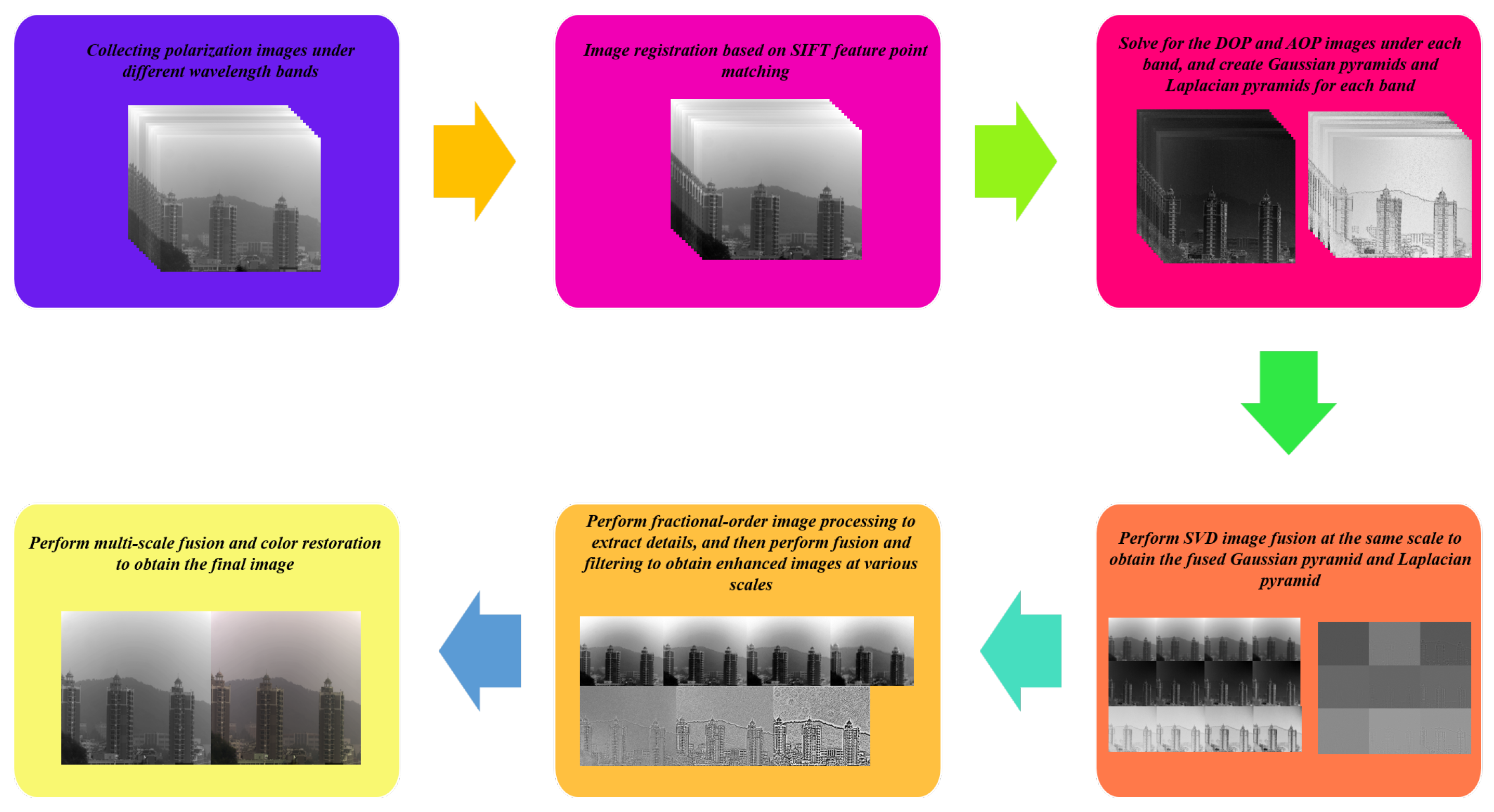
As shown in Figure 1, the process begins with the acquisition of polarization images in different spectral bands using a time-division polarization spectroscopy system. Subsequently, the SIFT feature matching algorithm is employed for image registration, yielding multi-band polarization images with pixel-level spatial correspondence. The Stokes vectors are then used to compute the DOP and AOP. Following this, Gaussian and Laplacian pyramids are constructed for the intensity, DOP, and AOP images in each band. Image fusion is then performed using SVD, where images from all bands at each scale are combined into a single fused image containing the integrated information, thereby creating fused Gaussian and Laplacian pyramids. Fractional-order image processing is applied to the fused images at each scale to enhance image details. Subsequently, detail enhancement and noise removal are carried out using self-guided filtering. Finally, multi-scale fusion is performed to obtain the final fused and enhanced image, followed by color restoration.

3.1. System Construction and Calibration

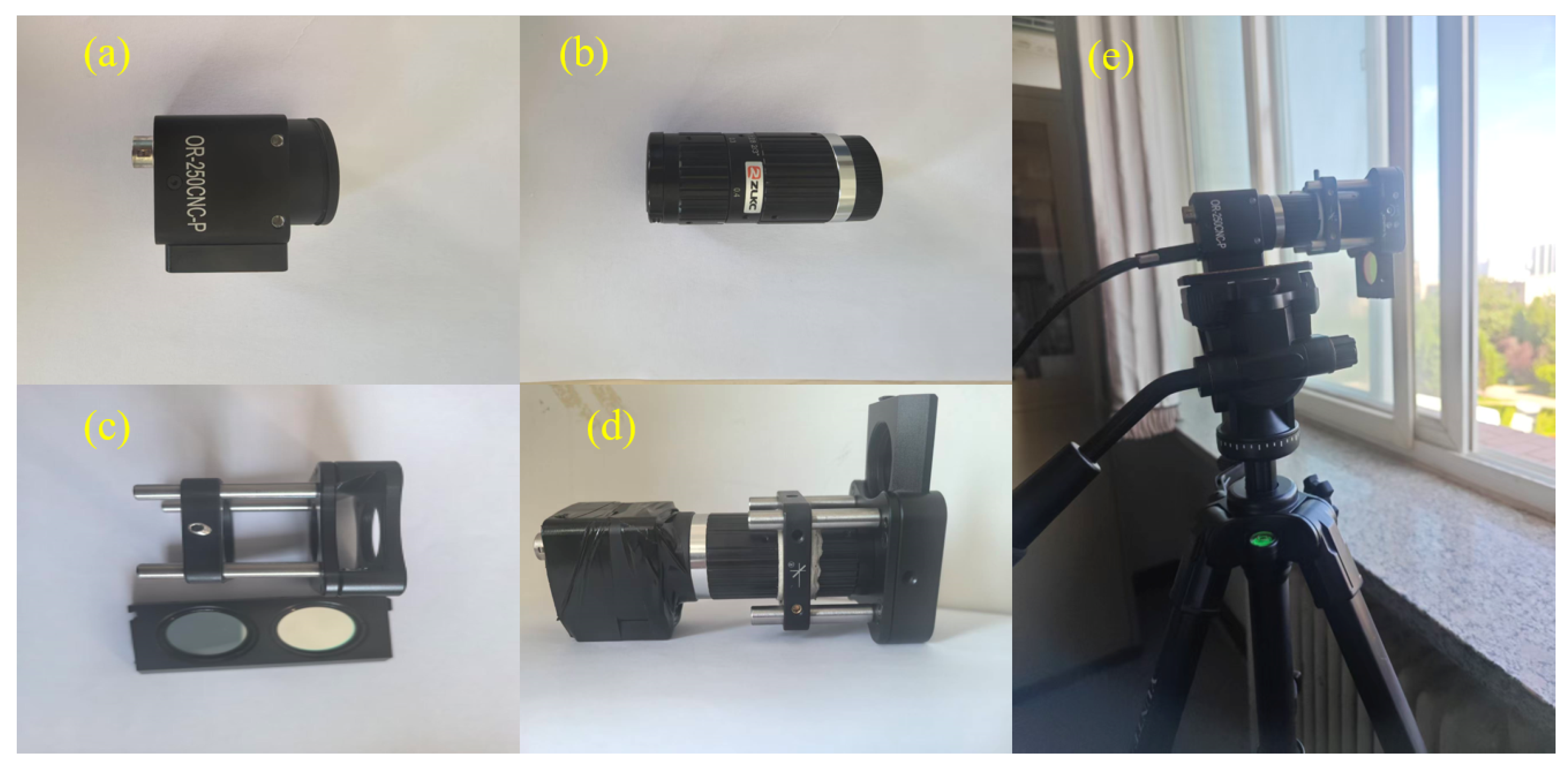
To enable polarization spectral image data acquisition in multiple scenarios, this paper constructs a time-division polarization spectral system. As shown in Figure 2a, the camera used is an OR-250CNC-P polarization camera, which outputs images with a resolution of 2448 × 2048. The adjacent four pixels within the camera sensor are arranged in a 2 × 2 pattern, corresponding to the output polarization image information. As shown in Figure 2b, the lens is a 50 mm fixed-focal-length lens. An optical cage plate, illustrated in Figure 2c, is used to secure the filter in front of the lens, resulting in the time-division polarization spectral camera depicted in Figure 2d. The camera position is fixed using a tripod and a gimbal. The final time-division polarization spectral system, shown in Figure 2e, ensures maximum precision in data acquisition under relatively stable conditions.
The bands of the filters selected in this paper are within the visible light spectrum, specifically 450 nm, 467 nm, 488 nm, 500 nm, 514 nm, 532 nm, 540 nm, 562 nm, 568 nm, 590 nm, 625 nm, and 660 nm. Due to variations in the transmittance of different filters and the camera sensor’s response to light intensity across different bands, it is necessary to calibrate the time-division polarization spectral system to accurately restore the spectral information of the object. An integrating sphere is chosen as the light source for system calibration because of its uniform brightness and non-polarized light output. For each band, multiple images are captured at different exposure times and brightness levels, and their average values are calculated. The corresponding average values of multiple dark-field images are subtracted. Fitting is then performed using the formula shown in Equation (22).
S λ = L L D a r k K λ t
where S λ represents the brightness of the band, L denotes the response of the camera sensor, L D a r k represents the dark-field noise, K λ is the gain factor for different bands, and t is the exposure time. The value of K λ is determined by fitting using Equation (22). Finally, the k λ values for different bands are shown in Table 1.

3.2. Data Preprocessing

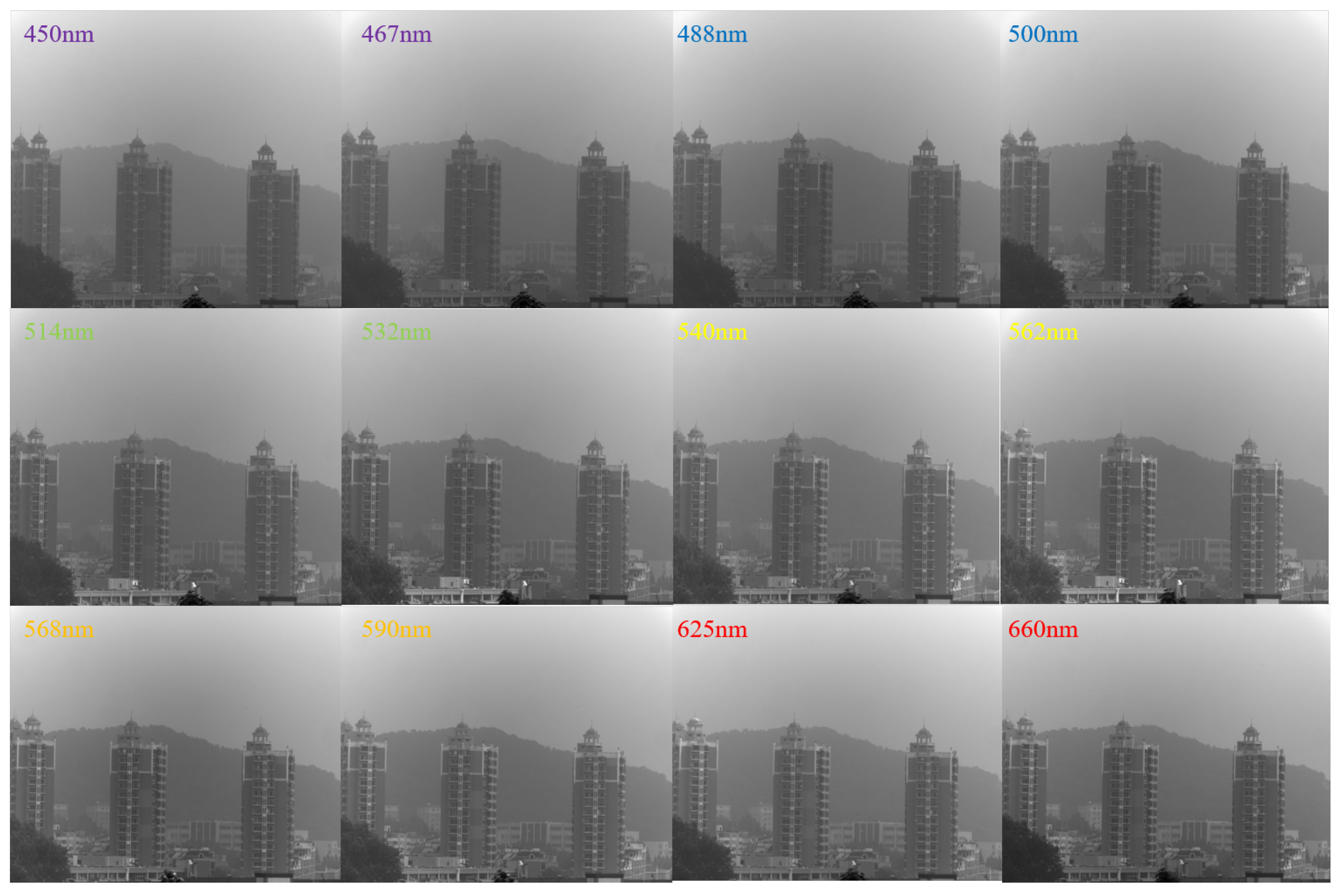
During the data acquisition process, it is necessary to continuously switch the filters of the time-division polarization spectroscopy system to obtain polarization images in different spectral bands. Due to the inherent limitations of the time-division polarization spectroscopy system, multi-band information cannot be acquired simultaneously but is obtained at different times. As a result, some spatial misalignment inevitably occurs. Figure 3 shows the original data image acquired by the time-division polarization spectroscopy system.
During the acquisition process, spatial misalignment errors arise from scene motion caused by temporal factors and vibration errors induced by filter switching, while the polarization spectral camera itself remains stationary. Therefore, we employ a feature point-based image registration algorithm to eliminate spatial misalignment. In image processing, various methods exist for calculating image feature points. To enhance registration accuracy, this paper selects the SIFT algorithm for feature point matching. The SIFT algorithm is a local feature description algorithm in image processing, known for its excellent stability and invariance. It adapts well to rotations, scale scaling, and brightness variations, while demonstrating strong robustness against interference. Consequently, we utilize the SIFT algorithm to compute feature points for each spectral band image. These feature points are then used to calculate the homography matrix between adjacent band images, followed by affine transformation. Overlapping regions are cropped, and the process repeats: matching features between the cropped region and the next band image. Ultimately, this yields registered images with precise spatial correspondence, as shown in Figure 4.
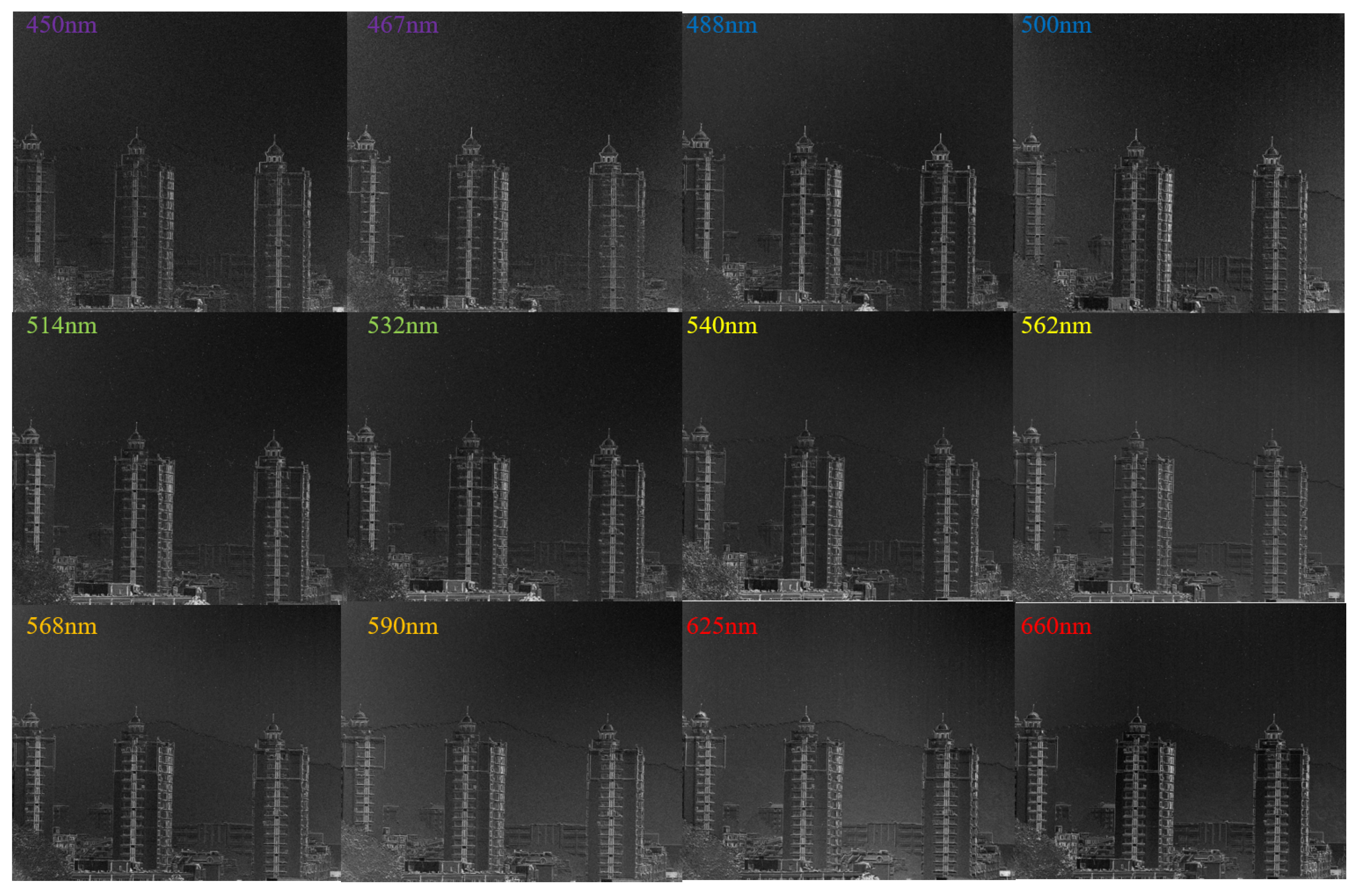
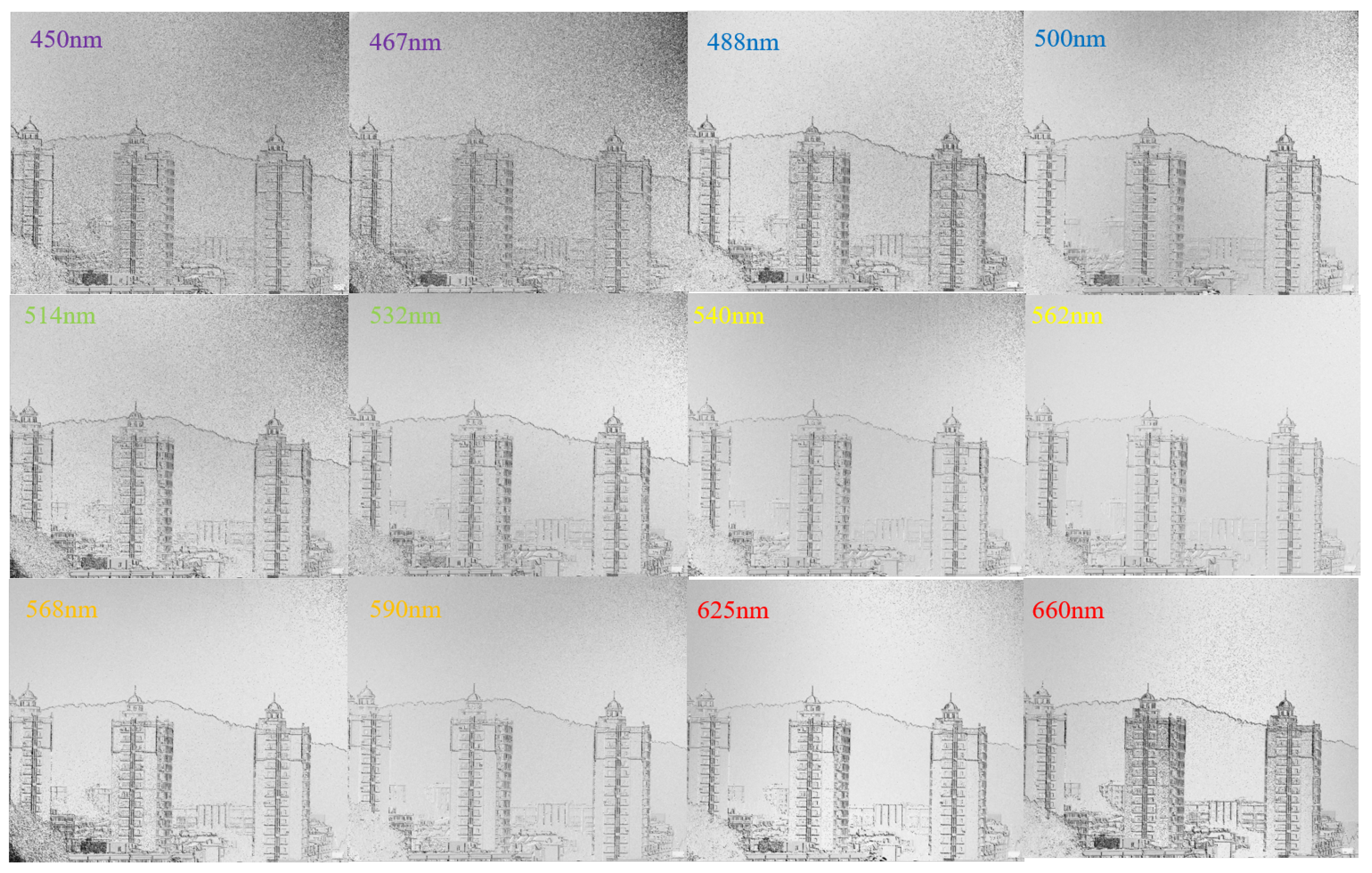
After image registration, DOP and AOP for different spectral bands are calculated according to Equations (6) and (7), based on the arranged polarizing elements array. Subsequently, through normalization, the value range of DOP, [0.0, 1.0], is linearly mapped to the image grayscale interval [0.0, 1.0]; similarly, the value range of AOP, [0, π ], is mapped to [0.0, 1.0]. As shown in Figure 5, these are the DOP images for different spectral bands. Figure 6 presents the AOP images corresponding to these bands.
Through observation of Figure 5 and Figure 6, it is found that the DOP and AOP vary across different spectral bands, revealing the polarization characteristics of the target in these bands. Therefore, it is necessary to effectively fuse the information from different bands using the algorithm proposed in this paper.

3.3. Polarization Multispectral Image Fusion

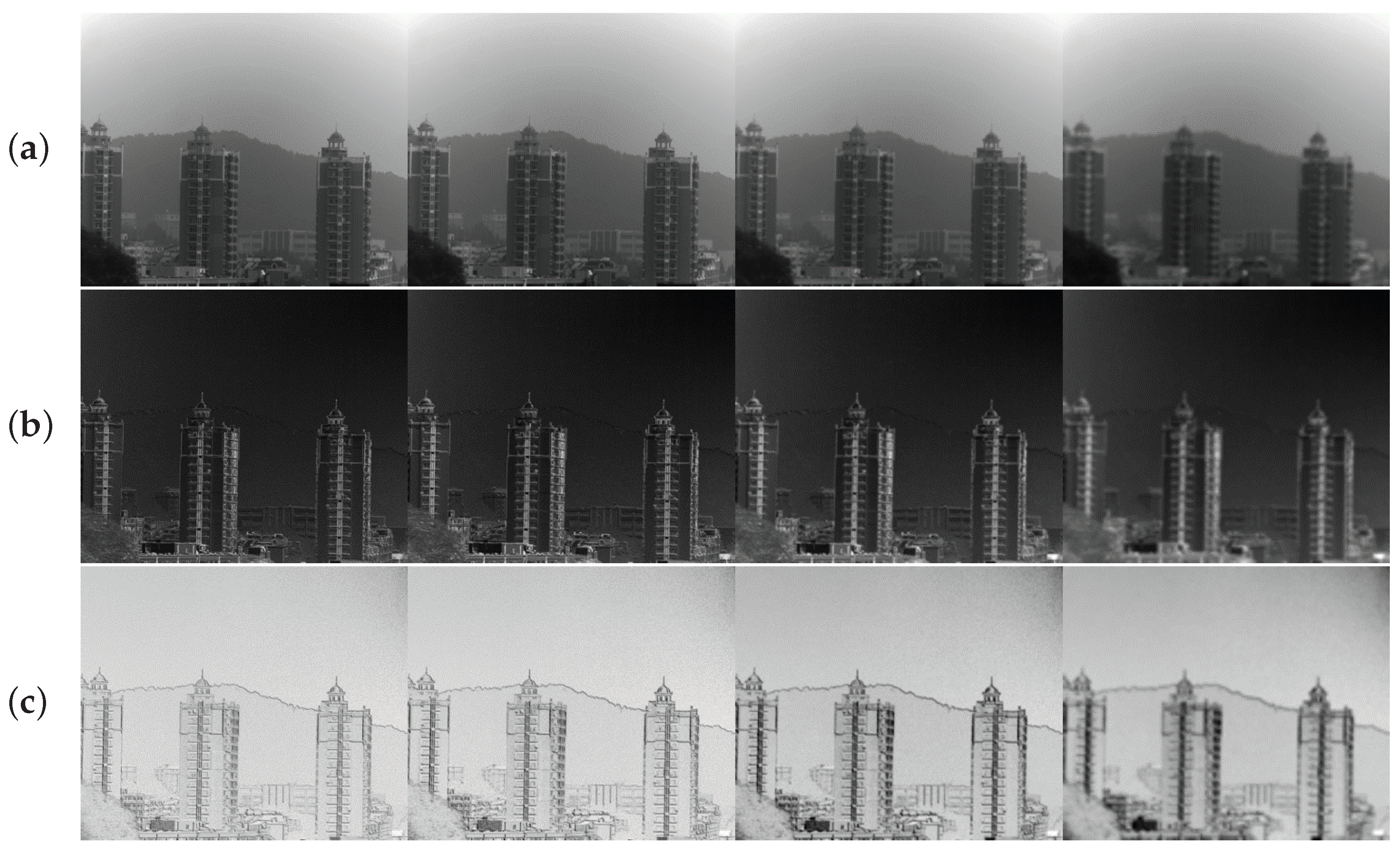
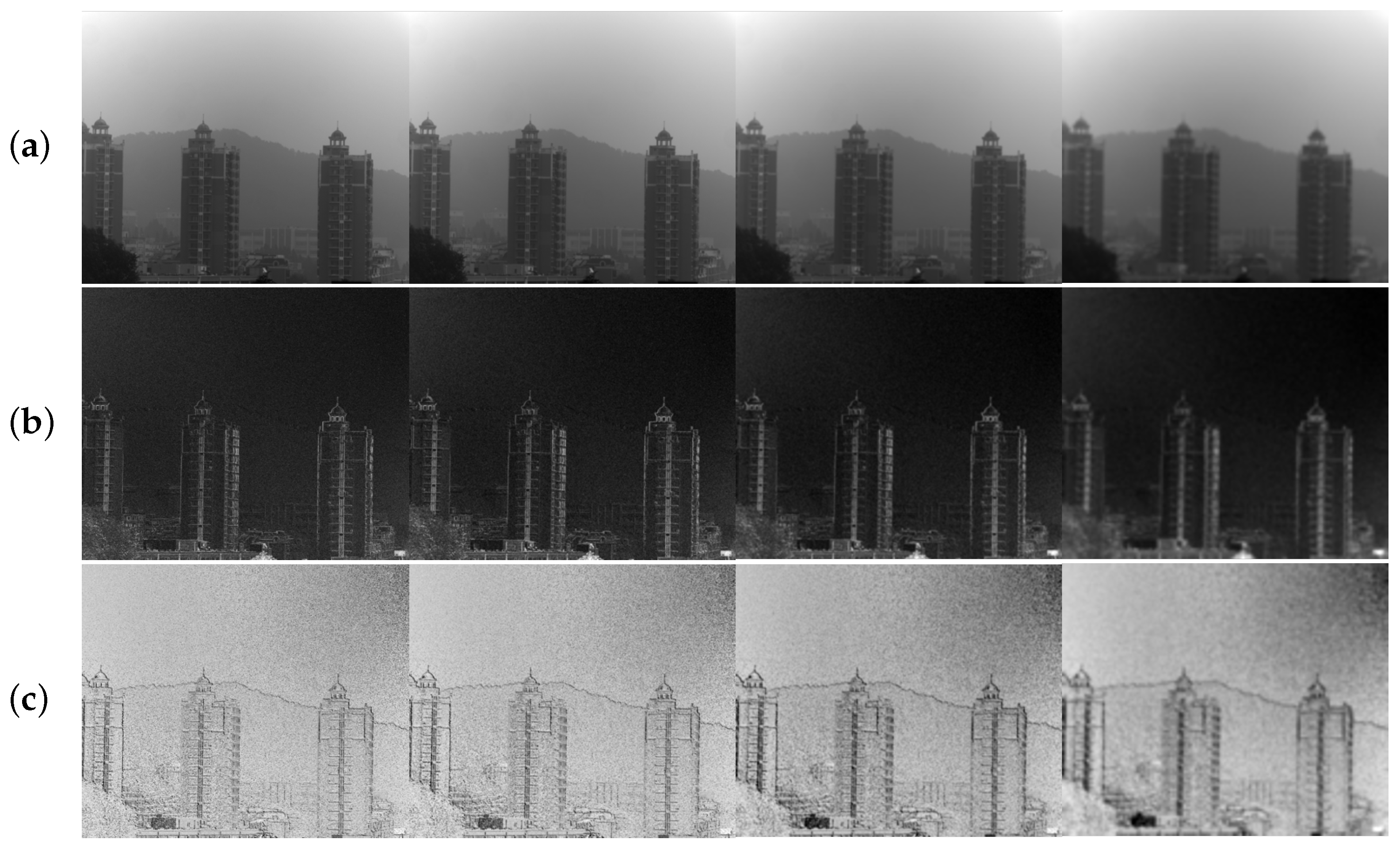
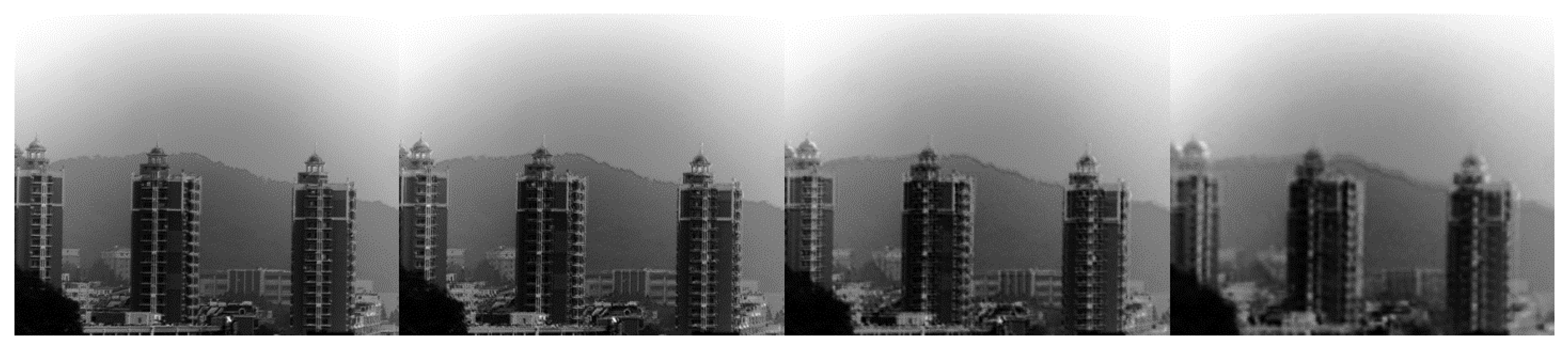
After obtaining fully registered polarization spectral image data, we proceed with the fusion of polarization multispectral images. Based on the theory in Section 2, we first perform multi-scale decomposition of the intensity information and polarization information of different bands using Equation (17). To ensure that the lowest scale still retains certain information, we set the minimum scale to no less than 100 × 100 pixels. Therefore, for the data in this paper, we selected a 4-layer Gaussian pyramid and a 3-layer Laplacian pyramid.As shown in Figure 7, Figure 7a is the Gaussian pyramid of light intensity, Figure 7b is the Gaussian pyramid of the degree of polarization, and Figure 7c is the Gaussian pyramid of the angle of polarization.
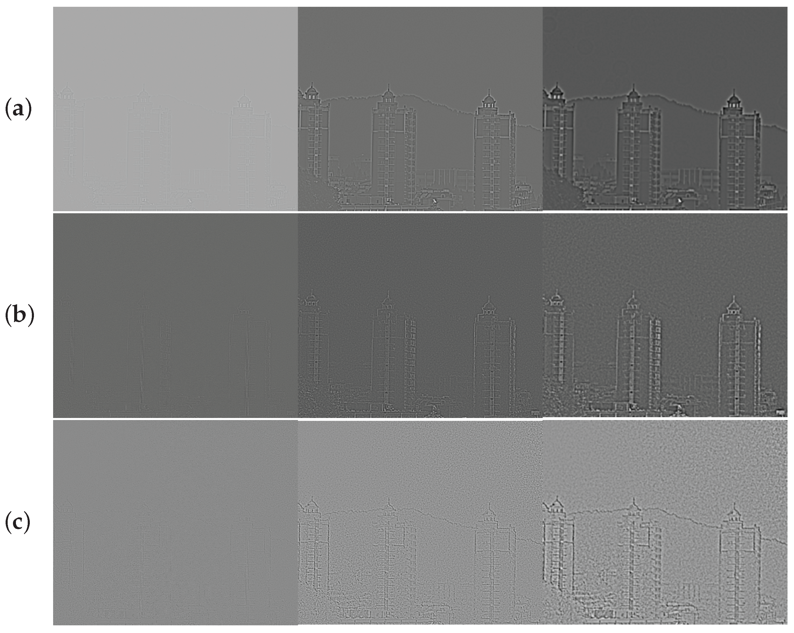
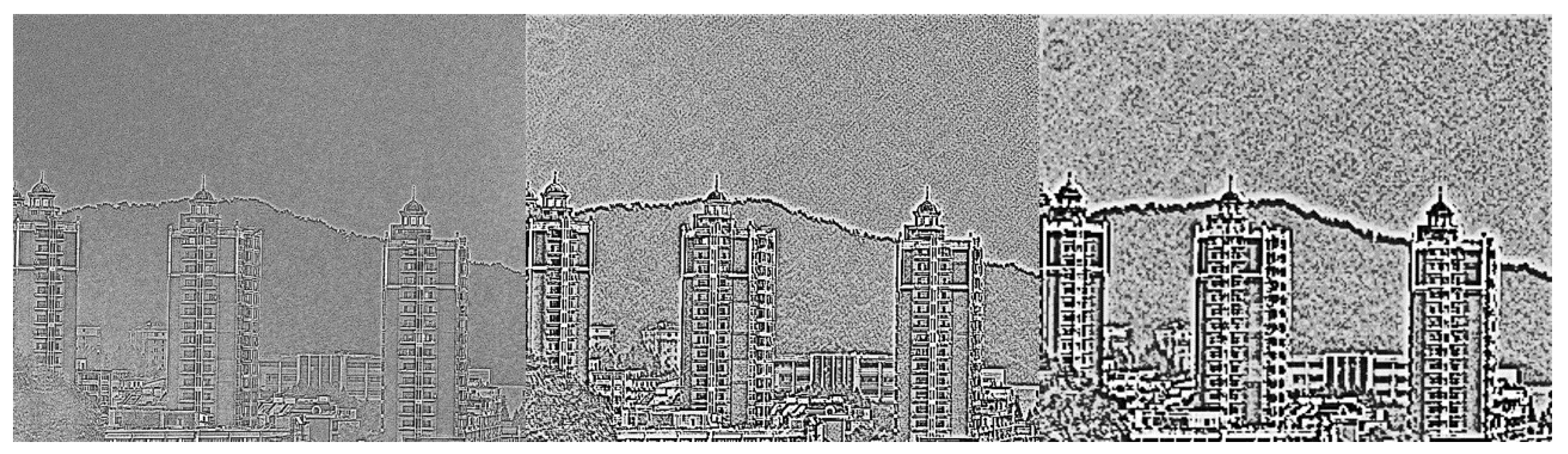
After obtaining the Gaussian pyramid, we can solve for the Laplacian pyramid of intensity information and polarization information under different bands according to Equation (17). As shown in Figure 8, Figure 8a is the Laplacian pyramid of the intensity image, Figure 8b is the Laplacian pyramid of the degree of polarization band, and Figure 8c is the Laplacian pyramid of the angle of polarization.
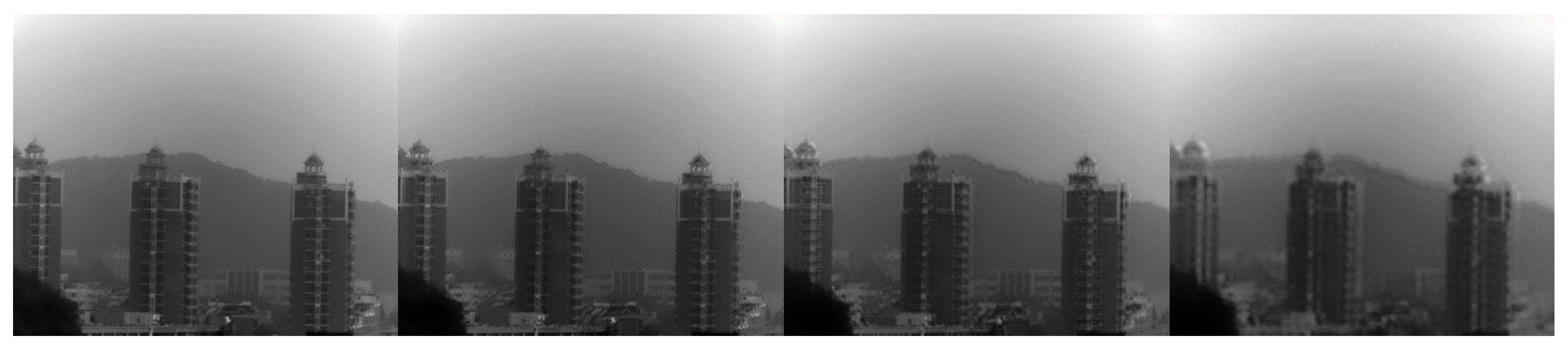
By performing multi-scale decomposition on the intensity information and polarization information of different bands, we obtained their Gaussian pyramids and Laplacian pyramids. Using Equation (17), we performed image fusion on the Gaussian pyramids and Laplacian pyramids of intensity, degree of polarization, and angle of polarization, respectively, to obtain the fused Gaussian pyramids of different information as shown in Figure 9.
Among them, Figure 9a is the fused Gaussian pyramid of intensity information, Figure 9b is the fused Gaussian pyramid of the degree of polarization, and Figure 9c is the fused Gaussian pyramid of the angle of polarization. To gain a more intuitive understanding of the image fusion effect, we evaluated it by calculating the contribution of the maximum features. As shown in Table 2, the contribution of the maximum features is mostly greater than 80%, indicating that the fused image retains most of the feature information from all bands.
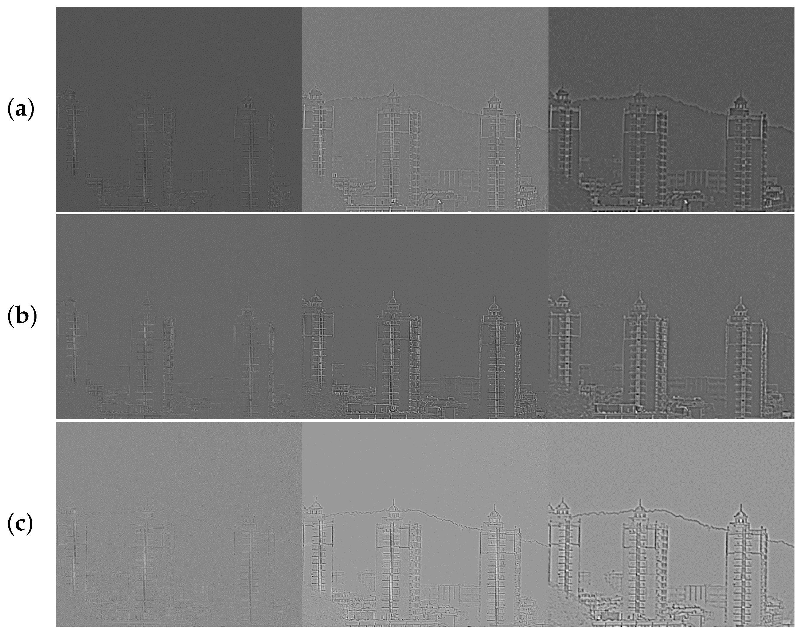
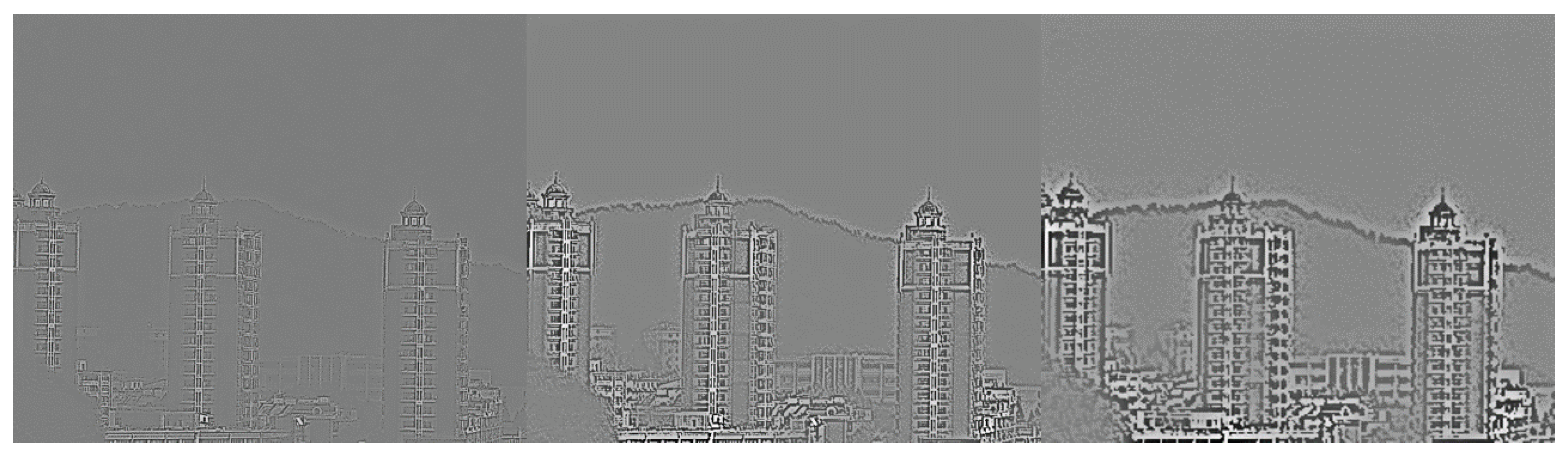
Next, we performed image fusion again on the Laplacian pyramids of intensity, degree of polarization, and angle of polarization across different bands, as shown in Figure 10. Among them, Figure 10a is the fused Laplacian pyramid of intensity information, Figure 10b is the fused Laplacian pyramid of the degree of polarization, and Figure 10c is the fused Laplacian pyramid of the angle of polarization.
Then, by calculating the contribution of the maximum features, as shown in Table 3, we found that in the high-scale layers, the contribution rate of the maximum features of the polarization information did not exceed 50%, indicating that some high-frequency information was lost during the fusion process. Therefore, in the subsequent processing, we need to enhance these high-frequency components.
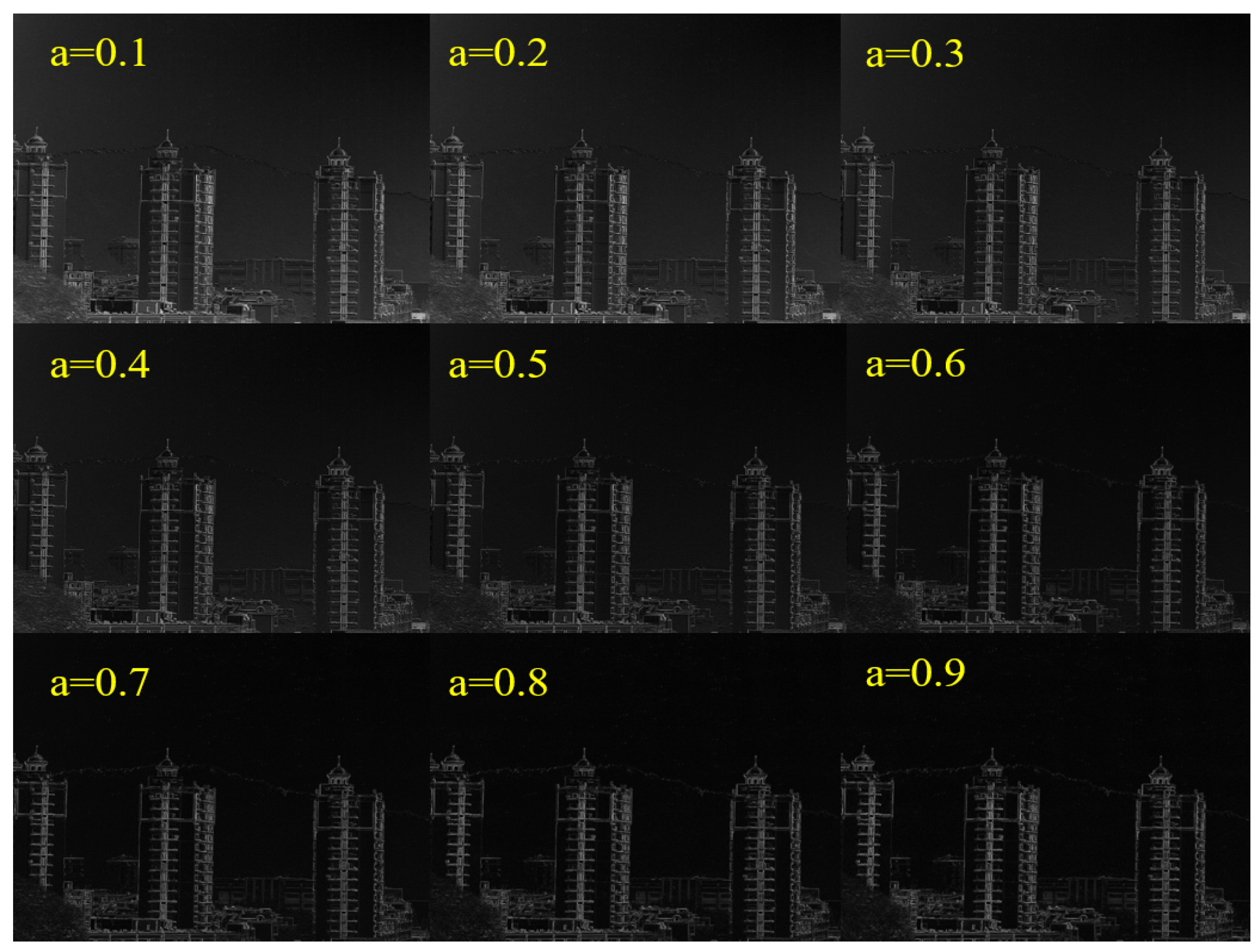
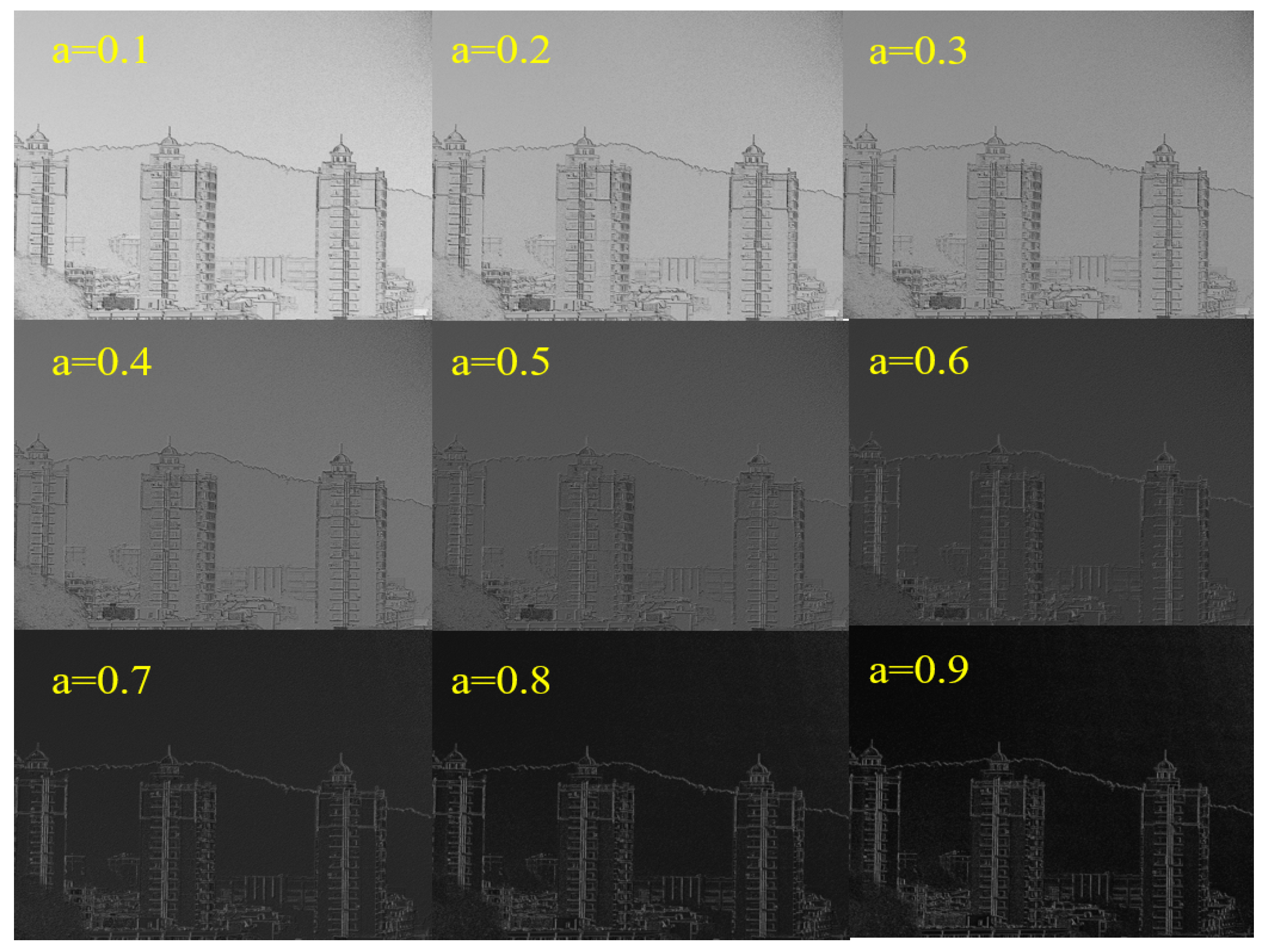
To further ensure the quality of image fusion, we solve for the fractional-order detail image using Equation (18). Fractional-order differentiation allows us to both extract the texture details of the image and enhance its high-frequency components, thereby addressing the loss of high-frequency information caused by the previous SVD fusion. To ensure computational accuracy and time efficiency, we select the first five terms of Equation (14) for the calculation. As illustrated in Figure 11 and Figure 12, different fractional orders a produce varying effects. When a = 0.1 , the texture details of the degree of polarization are significantly enhanced, while when a = 0.7 , the texture details of the angle of polarization are substantially improved. Therefore, in this paper, a = 0.1 is chosen as the fractional-order differentiation factor for the degree of polarization, and a = 0.7 is chosen as the fractional-order differentiation factor for the angle of polarization.
After determining the fractional-order differentiation factors, we perform image fusion between different types of information using Equation (19), and determine the specific coefficients λ 1 , μ 1 , ϕ 1 , λ 2 , μ 2 , ϕ 2 through Equation (21). To ensure the structural similarity of the images, we set the threshold T to 0.85. Ultimately, we obtain the Gaussian pyramid fractional-order fusion image and the Laplacian fractional-order fusion image, as shown in Figure 13 and Figure 14, which lays the foundation for subsequent multi-scale fusion. It can be observed from the Figure that the texture details have been significantly enhanced.
However, during the fusion process, noise interference is inevitably introduced. Therefore, we adopt a corresponding filtering method to remove the noise. The filtering method employed in this paper is guided filtering, which injects the aforementioned detail maps into the intensity image. Compared with traditional filtering methods, guided filtering offers several advantages in image processing tasks such as denoising, detail enhancement, image fusion, HDR, and dehazing. It preserves edges effectively without causing edge blurring, while simultaneously enhancing textures and details. The Gaussian fractional-order filtered image is shown Figure 15 and Figure 16.
Finally, we need to perform multi-scale image fusion to integrate the enhanced images from different scales into a single image at the same scale. To achieve this, we adopt the method described in Equation (20) for multi-scale fusion. The images are progressively reconstructed from the lowest scale to higher scales. To ensure that the features of each image are preserved during fusion, Equation (21) is used to enable adaptive selection while maintaining the threshold T > 0.85 . Ultimately, the fused image is obtained, as shown in Figure 17.

3.4. Color Restoration

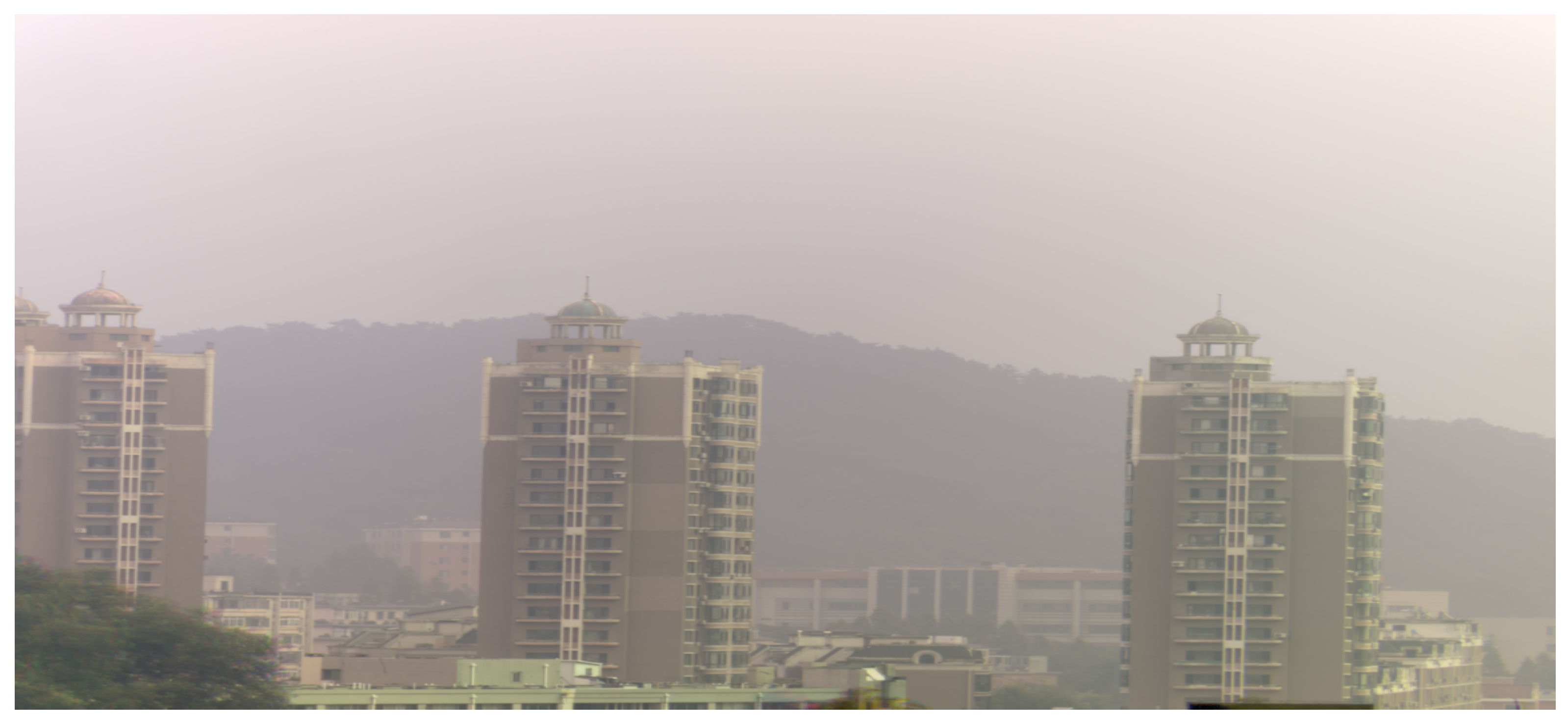
There are three types of cone photoreceptor cells in the human retina, which are sensitive to long waves (L, red), medium waves (M, green), and short waves (S, blue), respectively. The RGB sensors of color cameras are designed to simulate this response characteristic of the human eye. Therefore, based on the principles of color science and the response characteristics of typical imaging sensors, and since the three central wavelengths corresponding to the RGB color model are 450 nm (blue), 550 nm (green), and 650 nm (red), we selected 450 nm (blue), 562 nm, and 660 nm from our spectral bands. Finally, we reconstructed an image with color information, as shown in Figure 18.
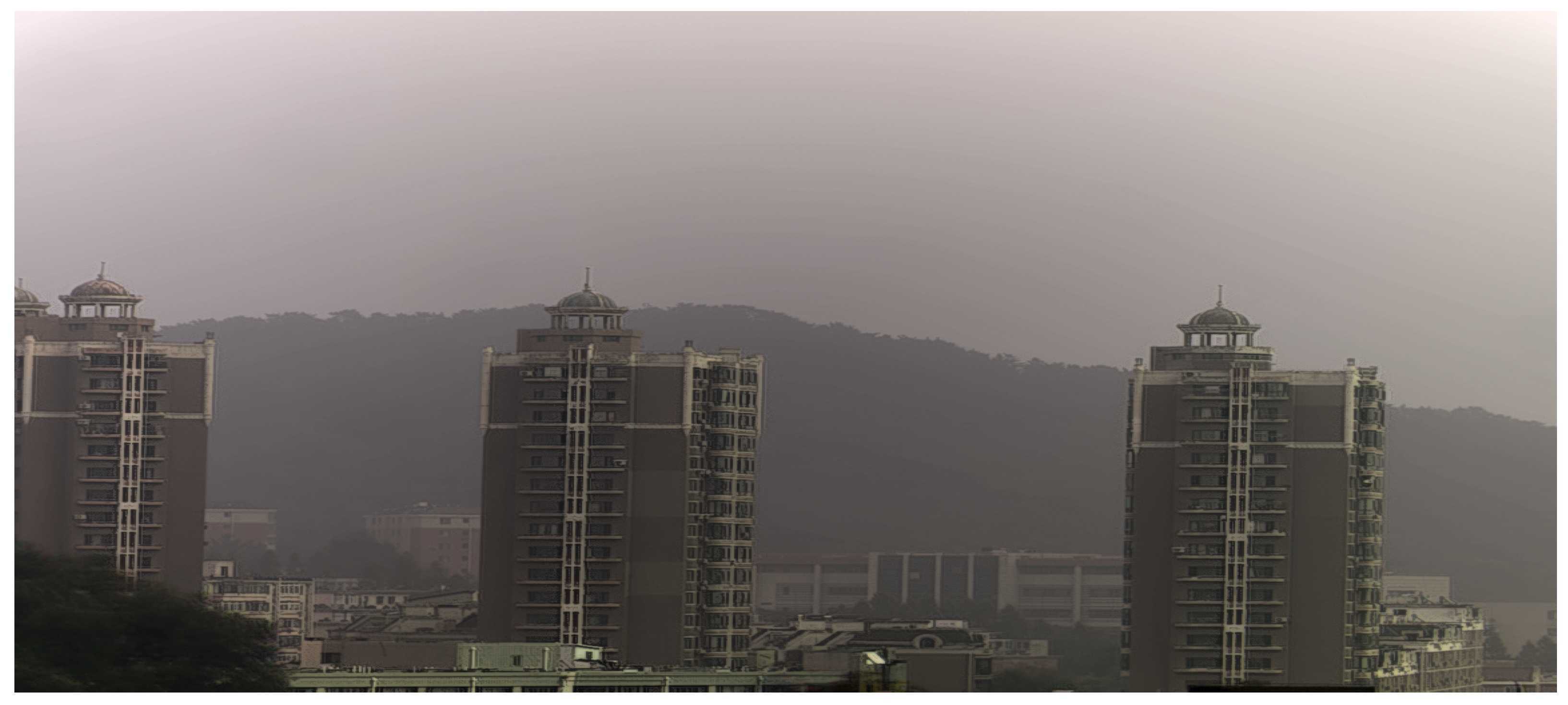
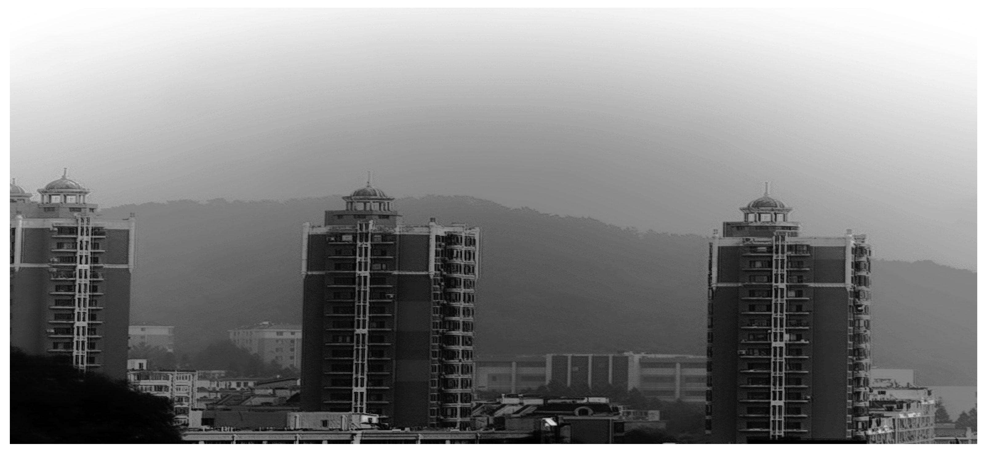
At the same time, we can inject the luminance information from the grayscale version of the fused image into the color image while preserving the original colors of the color image. To achieve this, we convert the color image to the HSV color space, separate the channels, replace the V channel with the fused grayscale image, merge the channels, and then convert back to the RGB image. Finally, the resulting fused color image is obtained, as shown in Figure 19.

4. Result Analysis

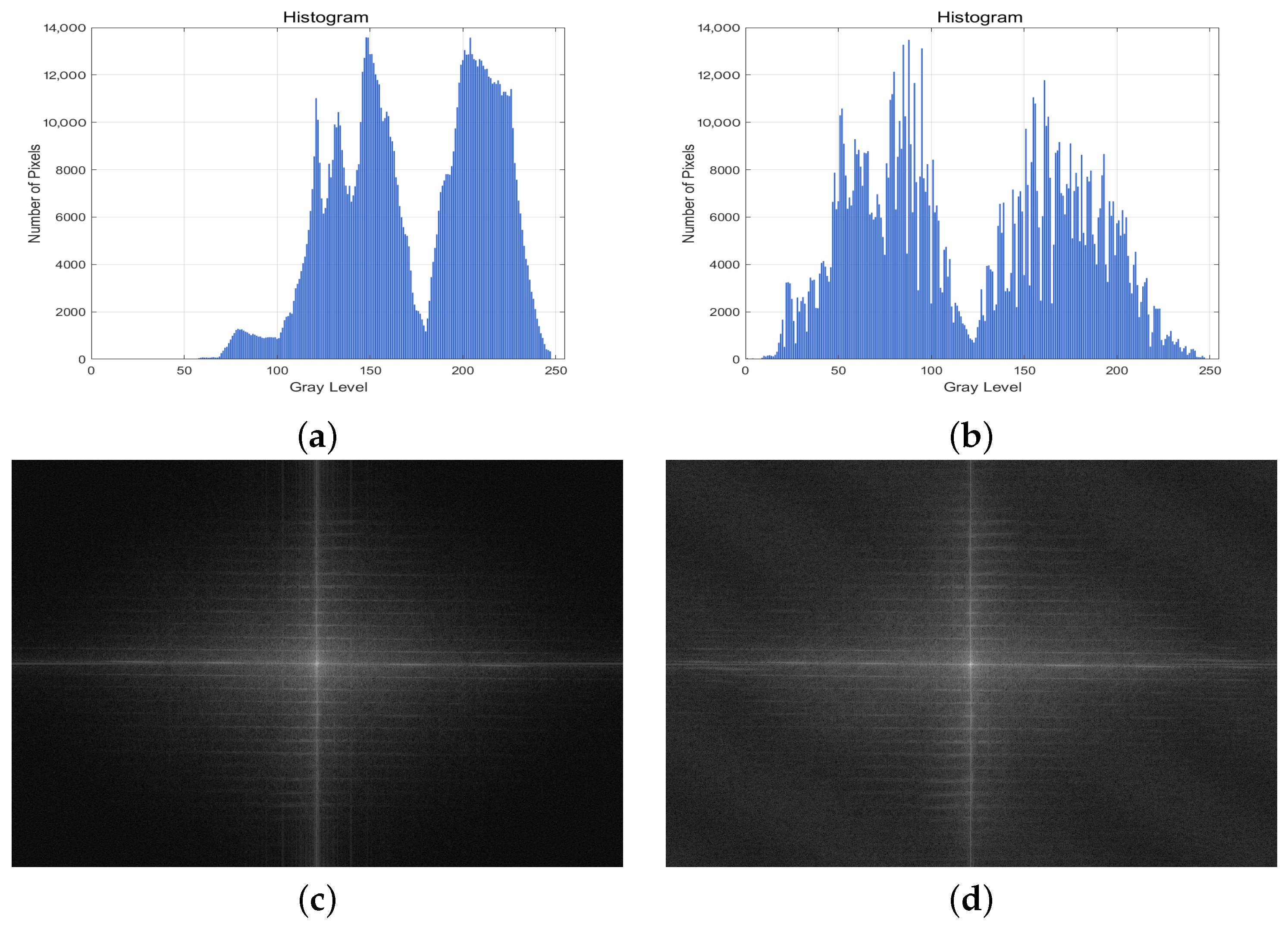
To verify the error and accuracy of the algorithm proposed in this paper, we conducted histogram analysis and spectral analysis on Figure 18 and Figure 19 respectively. The histogram is used to compare the deviation in pixel distribution of the images before and after fusion, thus reflecting the fidelity of brightness and contrast. Spectral analysis is used to evaluate the preservation of details in different frequency bands and the potential introduction of spectral distortion. The analysis results are shown in Figure 20.
From the analysis of the gray-level histogram, it can be seen that Figure 20b has a more complete dynamic range and a more balanced distribution of light and dark areas, with both dark and bright information well preserved. Overall, it presents a more natural bimodal structure. On the other hand, the gray-level distribution of Figure 20a is noticeably shifted towards medium and high gray levels, with serious loss of dark information, resulting in a compressed overall dynamic range. Therefore, from the perspective of information integrity, Figure 20b is superior to Figure 20a.
Figure 20c,d are both centered Fourier transform amplitude spectra of the image. The core commonality between the two is the presence of a bright spot at the center representing the average brightness of the image, and both have cross shaped bright lines reflecting the horizontal and vertical structure and edge discontinuity of the image; The core difference lies in the fact that the cross shaped bright lines in Figure 20d are thinner and sharper, the background is cleaner, and the energy attenuation is faster, corresponding to a regular structure, lower noise, and higher information purity in the original image; The cross lines in Figure 20c are thicker, the energy diffusion range is larger, and the background is covered with dense noise textures, corresponding to higher frequency noise or richer microscopic details in the original image. However, the overall purity and structural regularity are weaker than those in the first image.
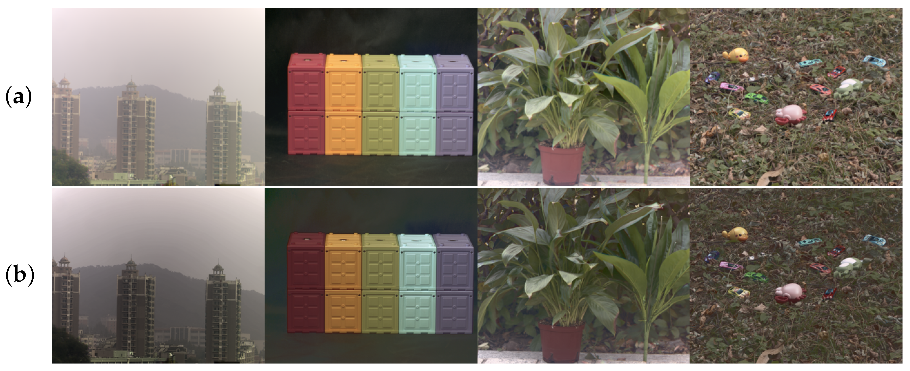
To further verify the effectiveness of the algorithm proposed in this paper, we compare it with other algorithms in different scenarios, as shown in Figure 21. Figure 21a presents the original spectral color images in different scenarios, while Figure 21b shows the fused color images in the corresponding scenarios. From Figure 21, it can be observed that in different scenarios, the texture details of the images fused by the algorithm proposed in this paper are significantly improved compared to the original images. The image quality is notably enhanced.
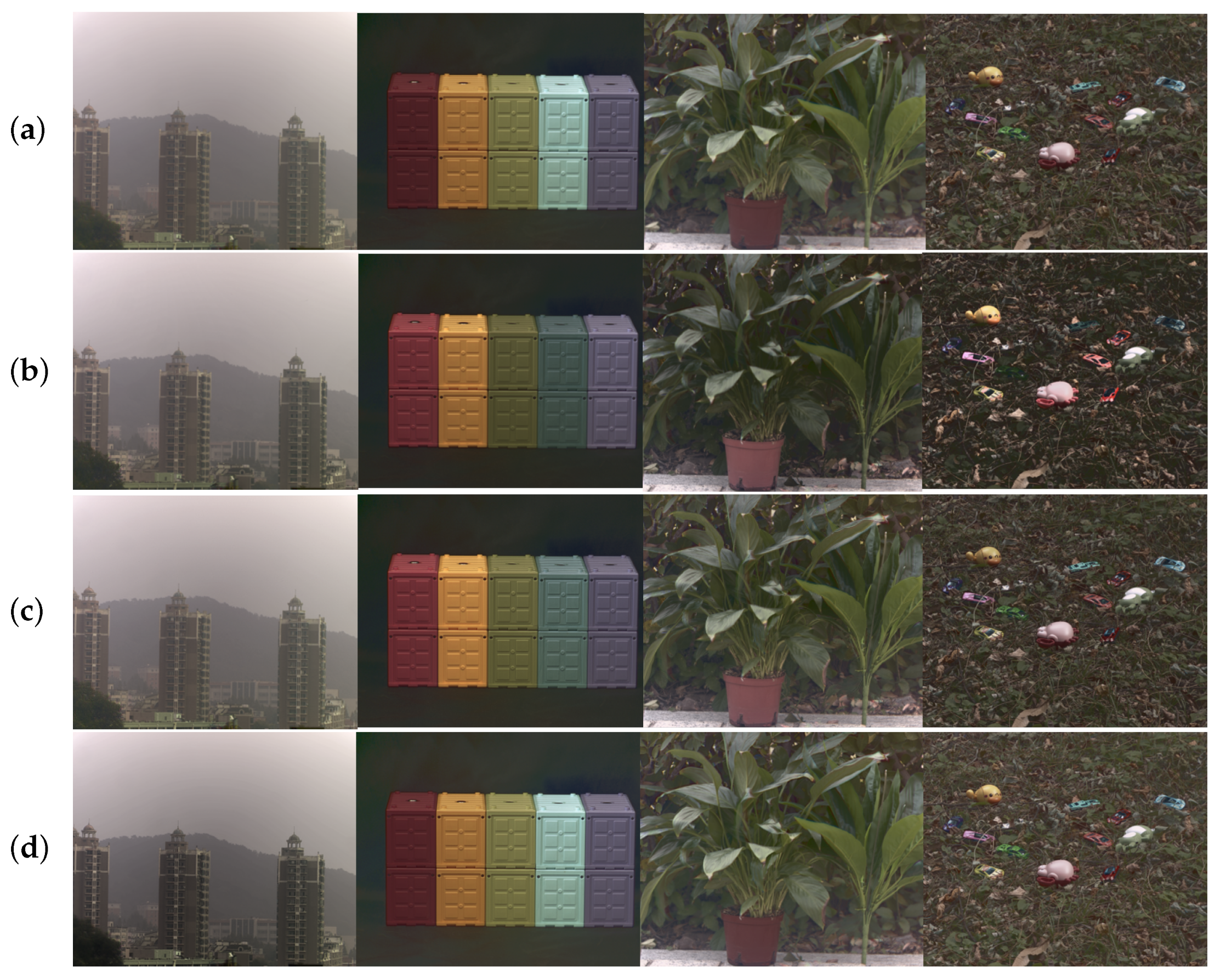
To further demonstrate the effectiveness of the algorithm proposed in this paper, it is also compared with commonly used image fusion algorithms, as shown in Figure 22. Figure 22a presents the PCA fused color images in different scenarios, Figure 22b shows the Poisson fusion color images in different scenarios, Figure 22c displays the NSCT fused color images in different scenarios, and Figure 22d presents the fused color images obtained by the proposed algorithm in different scenarios. From Figure 22, it can be observed that although the PCA fusion algorithm can process multispectral images efficiently, the texture details in the fused images are not prominent. The Poisson fusion algorithm, a gradient-domain-based method, performs image fusion based on luminance transformation; while details are improved, color distortion is severe. The NSCT algorithm, a multi-scale analysis method, achieves relatively high fusion quality but may introduce artifacts and blurring in certain scenarios. In contrast, the algorithm proposed in this paper not only preserves color fidelity but also significantly enhances texture details, greatly improving image quality.
To more objectively reflect image quality, we adopt four image evaluation metrics—information entropy [32], average gradient [33], image standard deviation [34], and SSIM—to assess image quality [35]. As shown in Table 4, the proposed algorithm, while maintaining maximum image similarity, achieves the highest information entropy, average gradient, and standard deviation in most scenarios, further demonstrating its effectiveness.

5. Conclusions and Prospect

This paper proposes a multi-scale image fusion algorithm based on polarization spectral images, which achieves favorable fusion results even in multi-scene and multi-target backgrounds. First, through multi-scale decomposition, the polarization images of different bands are transformed into Gaussian pyramids and Laplacian pyramids. For the multi-band images at different pyramid scales, fusion is performed using SVD to obtain fused Gaussian and Laplacian pyramids. Fractional-order processing is then applied to extract detailed textures from the images, followed by guided filtering for noise filtering. Subsequently, through the fusion strategy proposed in this paper, the images are progressively fused and reconstructed back to the original image scale, yielding the final fused image. While ensuring maximum structural similarity, this method significantly enhances the fusion details and guarantees the quality of the fused image. Although the proposed algorithm achieves good fusion performance, there are still some limitations that require improvement in future work.
  • The proposed method relies heavily on the accuracy of image registration. For moving objects, perfect registration cannot always be achieved, which may lead to artifacts and overlapping in the subsequent image fusion process, thereby degrading the fusion quality.
  • The algorithm depends on multi-scale image processing, which is time-consuming. Its time complexity and space complexity are relatively high compared to other algorithms.
  • The proposed algorithm is suitable for high-resolution images. For low-resolution images, continuous scale changes may lead to degradation in the quality of the fused image.

Author Contributions

Conceptualization, Z.Z. and X.C.; methodology, X.C.; software, Z.W.; valida tion, Z.Z. and X.C.; formalanalysis, Z.W.; investigation, X.C.; resources, X.C.; datacuration, Z.W.; writing—original draft preparation, Z.W.; writing—review and editing, Z.Z., X.C. and Z.W.; visualization, X.C.; supervision, X.C.; projectadministration, Z.Z.; funding acquisition, Z.Z. All authors have read and agreed to the published version of the manuscript.

Funding

This research received no external funding.

Institutional Review Board Statement

Not applicable.

Informed Consent Statement

Not applicable.

Data Availability Statement

The raw data supporting the conclusions of this article will be made available by the authors on request.

Conflicts of Interest

The authors declare no conflicts of interest.

References

  1. Liu, S.; Liu, X.; Yuan, J.; Bao, J. Multidimensional Information Encryption and Storage: When the Input Is Light. Research 2021, 2021, 7897849. [Google Scholar] [CrossRef] [Scilit]
  2. Yi, J.; Jiang, H.; Tan, Y. The Detection of Soybean Bacterial Blight Based on Polarization Spectral Imaging Techniques. Agronomy 2025, 15, 50. [Google Scholar] [CrossRef] [Scilit]
  3. Kim, D.; Vamara, D. One-piece polarizing interferometer for ultrafast spectroscopic polarimetry. Sci. Rep. 2019, 9, 5978. [Google Scholar] [CrossRef] [Scilit] [PubMed]
  4. Liu, Z.; Song, Z.; Li, Z.; Li, L. Integrated Polarimetric Spectral Imaging Sensor Combining Spectral Imaging and Polarization Modulation Techniques. Sensors 2026, 26, 144. [Google Scholar] [CrossRef] [Scilit]
  5. Liu, J.; Cui, J.; Chen, M.; Yang, S.; Sun, H.; Wang, Q.; Zhan, J.; Li, Y.; Fu, Q.; Wang, C. Design of Polarization Spectroscopy Integrated Imaging System. Photonics 2024, 11, 1183. [Google Scholar] [CrossRef] [Scilit]
  6. Yan, C.; Zhang, Y.; Bo, J.; Ju, X.; Yu, B.; Li, X. Development and prospect of hyperspectral polarization. Opt. Precis. Eng. 2024, 32, 2141–2165. [Google Scholar] [CrossRef] [Scilit]
  7. Prasad, N.S.; Jin, F.; Haskovic, E.Y.; Kutcher, S.; Trivedi, S.B.; Soos, J. Acousto-optic tunable filter based spectrapolarimeter for extraction of Stokes and Mueller matrices. In Proceedings of the Polarization: Measurement, Analysis, and Remote Sensing XIII; Chenault, D.B., Goldstein, D.H., Eds.; International Society for Optics and Photonics, SPIE: Bellingham, WA, USA, 2018; Volume 10655, p. 106550A. [Google Scholar] [CrossRef] [Scilit]
  8. Chen, L.; Zhang, S.; Zheng, W.; Yao, L. High Light Efficiency Spectral Polarization Imaging Method Based on Mach–Zehnder Structured Liquid Crystal Tunable Filters and Variable Retarders. Photonics 2023, 10, 765. [Google Scholar] [CrossRef] [Scilit]
  9. Hu, C.; Wang, X.; Qi, Z.; Li, C. The new infrared beamline at NSRL. Infrared Phys. Technol. 2020, 105, 103200. [Google Scholar] [CrossRef] [Scilit]
  10. Gupta, N. Hyperspectral imager development at Army Research Laboratory. In Proceedings of the Infrared Technology and Applications XXXIV; Andresen, B.F., Fulop, G.F., Norton, P.R., Eds.; International Society for Optics and Photonics, SPIE: Bellingham, WA, USA, 2008; Volume 6940, p. 69401P. [Google Scholar] [CrossRef] [Scilit]
  11. Li, Q.; Lu, F.; Wang, X.; Zhu, C. Low crosstalk polarization-difference channeled imaging spectropolarimeter using double-Wollaston prism. Opt. Express 2019, 27, 11734–11747. [Google Scholar] [CrossRef] [Scilit]
  12. Zhang, F.; Liao, M.; Pu, M.; Guo, Y.; Chen, L.; Li, X.; He, Q.; Kang, T.; Ma, X.; Ke, Y.; et al. A Miniature Meta-Optical System for Reconfigurable Wide-Angle Imaging and Polarization-Spectral Detection. Engineering 2024, 35, 69–75. [Google Scholar] [CrossRef] [Scilit]
  13. Fan, A.; Xu, T.; Li, J.; Teng, G.; Wang, X.; Zhang, Y.; Xu, C. Compressive full-Stokes polarization and flexible hyperspectral imaging with efficient reconstruction. Opt. Lasers Eng. 2023, 160, 107256. [Google Scholar] [CrossRef] [Scilit]
  14. Zhu, W.; Zhai, L.; Du, W.; Li, X.; Gao, Z.; Wang, H.; Li, Y. Applications of Polarization Spectroscopy in Agricultural Engineering: A Comprehensive Review. Agriculture 2025, 15, 2546. [Google Scholar] [CrossRef] [Scilit]
  15. Zhang, G.; Li, S.; Lv, Q.; Wang, C. Research on hyperspectral polarization detection for unexploded ordnance target identification. In Proceedings of the 3rd International Conference on Laser, Optics, and Optoelectronic Technology (LOPET 2023); Li, X., Costa, M.F., Eds.; International Society for Optics and Photonics, SPIE: Bellingham, WA, USA, 2023; Volume 12757, p. 127570B. [Google Scholar] [CrossRef] [Scilit]
  16. Shi, H.; Gong, C.; Wang, Q.; Liu, J.; Wang, J.; Li, Y.; Sun, H.; Wang, C.; Ma, Y.; Kang, X.; et al. Airborne push-broom hyperspectral polarization imaging system design and image fusion method. Opt. Laser Technol. 2025, 191, 113409. [Google Scholar] [CrossRef] [Scilit]
  17. Zhang, Y.; Ju, X.; Yan, C.; Bo, J.; Li, X.; Zhang, J. Polarized hyperspectral image fusion method for targets in sea clutter background. Opt. Commun. 2025, 591, 131993. [Google Scholar] [CrossRef] [Scilit]
  18. Zhu, P.; Liu, Z.; Huang, Z. Infrared polarization and intensity image fusion based on DTCWT and sparse representation. Acta Photonica Sin. 2017, 46, 1210002. [Google Scholar] [CrossRef] [Scilit]
  19. Kaur, H.; Koundal, D.; Kadyan, V. Image Fusion Techniques: A Survey. Arch. Comput. Methods Eng. 2021, 28, 4425–4447. [Google Scholar] [CrossRef] [Scilit]
  20. Zhong, J.; Liu, X.; Wang, X.; Liu, J.; Liu, H.; Yuan, C.; Liu, Y.; Yu, T. Reconstruction and Fusion Algorithm for Polarization Spectral Multidimensional Information. Spectrosc. Spectr. Anal. 2023, 43, 1254–1261. [Google Scholar]
  21. Guo, F.; Zhu, J.; Huang, L.; Li, F.; Zhang, N.; Deng, J.; Li, H.; Zhang, X.; Zhao, Y.; Jiang, H.; et al. Multi-Dimensional Fusion of Spectral and Polarimetric Images Followed by Pseudo-Color Algorithm Integration and Mapping in HSI Space. Remote Sens. 2024, 16, 1119. [Google Scholar] [CrossRef] [Scilit]
  22. Meng, X.; Hu, Y.; Zhi, D. EDEFusion: Edge detail enhancement for infrared intensity and polarization image fusion with rolling guidance filtering and sparse representation. Signal Image Video Process. 2025, 19, 980. [Google Scholar] [CrossRef] [Scilit]
  23. Wang, J.; Zhu, X.; Jing, L.; Tang, Y.; Li, H.; Xiao, Z.; Ding, H. HyperGAN: A Hyperspectral Image Fusion Approach Based on Generative Adversarial Networks. Remote Sens. 2024, 16, 4389. [Google Scholar] [CrossRef] [Scilit]
  24. Karim, S.; Tong, G.; Li, J.; Yu, Y.; Ibrar, M.; Mehmood, F. Dense Network-Based Spectral-Polarization Image Fusion: Multispectral Data Enhancement via Encoder-Decoder Approach. In Proceedings of the 6th International Conference on Information Technologies and Electrical Engineering; Association for Computing Machinery: New York, NY, USA, 2024; pp. 441–446. [Google Scholar] [CrossRef] [Scilit]
  25. Tong, G.; Yao, X.; Li, B.; Fu, J.; Wang, Y.; Hao, J.; Karim, S.; Yu, Y. MSPFusion: A feature transformer for multidimensional spectral-polarization image fusion. Expert Syst. Appl. 2025, 275, 127079. [Google Scholar] [CrossRef] [Scilit]
  26. Zhang, J.; Shao, J.; Chen, J.; Yang, D.; Liang, B.; Liang, R. PFNet: An unsupervised deep network for polarization image fusion. Opt. Lett. 2020, 45, 1507–1510. [Google Scholar] [CrossRef] [Scilit] [PubMed]
  27. Wang, S.; Meng, J.; Zhou, Y.; Hu, Q.; Wang, Z.; Lyu, J. Polarization Image Fusion Algorithm Using NSCT and CNN. J. Russ. Laser Res. 2021, 42, 443–452. [Google Scholar] [CrossRef] [Scilit]
  28. Liu, J.; Duan, J.; Hao, Y.; Chen, G.; Zhang, H. Semantic-guided polarization image fusion method based on a dual-discriminator GAN. Opt. Express 2022, 30, 43601–43621. [Google Scholar] [CrossRef] [Scilit]
  29. Wan, Z.; Zhao, K.; Cheng, H.; Fu, P. Measurement Modeling and Performance Analysis of a Bionic Polarimetric Imaging Navigation Sensor Using Rayleigh Scattering to Generate Scattered Sunlight. Sensors 2024, 24, 498. [Google Scholar] [CrossRef] [Scilit]
  30. Fujino, T.; Takakura, S.; Arani, S.S.; Barron, D.; Baccigalupi, C.; Chinone, Y.; Errard, J.; Fabbian, G.; Feng, C.; Halverson, N.W.; et al. A Measurement of Atmospheric Circular Polarization with POLARBEAR. Astrophys. J. 2025, 981, 15. [Google Scholar] [CrossRef] [Scilit]
  31. Harmel, T. Apparent Surface-to-Sky Radiance Ratio of Natural Waters Including Polarization and Aerosol Effects: Implications for Above-Water Radiometry. Front. Remote Sens. 2023, 4, 1307976. [Google Scholar] [CrossRef] [Scilit]
  32. Liu, Y.; Huang, Z.; Yu, F.; Lin, G.; Zeng, J.; Ma, M.; Zhan, L.; Zhang, X. A novel image quality evaluation method based on two-dimensional information entropy. J. Phys. Conf. Ser. 2023, 2478, 062005. [Google Scholar] [CrossRef] [Scilit]
  33. Sung, J.-M.; Kim, D.-C.; Choi, B.-Y.; Ha, Y.-H. Image thresholding using standard deviation. In Image Processing: Machine Vision Applications VII; Niel, K.S., Bingham, P.R., Eds.; SPIE: Bellingham, WA, USA, 2014; Volume 9024, p. 90240R. [Google Scholar] [CrossRef] [Scilit]
  34. Li, W.; Hu, X.; Du, J.; Xiao, B. Adaptive remote-sensing image fusion based on dynamic gradient sparse and average gradient difference. Int. J. Remote Sens. 2017, 38, 7316–7332. [Google Scholar] [CrossRef] [Scilit]
  35. Horé, A.; Ziou, D. Image Quality Metrics: PSNR vs. SSIM. In Proceedings of the 2010 20th International Conference on Pattern Recognition; IEEE: New York, NY, USA, 2010; pp. 2366–2369. [Google Scholar] [CrossRef] [Scilit]
Figure 1. Algorithm flowchart of this paper.
Applsci 16 04087 g001
Figure 2. Experimental setup diagram: (a) is a polarization camera, (b) is a lens, (c) is an optical cage plate, (d) is a time-sharing polarization spectral camera, and (e) is a time-sharing polarization spectral acquisition system.
Applsci 16 04087 g002
Figure 3. Unregistered images of different bands.
Applsci 16 04087 g003
Figure 4. S 0 registration images of different bands.
Applsci 16 04087 g004
Figure 5. DOP registration images of different bands.
Applsci 16 04087 g005
Figure 6. AOP registration images of different bands.
Applsci 16 04087 g006
Figure 7. The Gaussian pyramid diagrams: (a) represents the light intensity pyramid, (b) represents the DOP pyramid, and (c) represents the AOP pyramid.
Applsci 16 04087 g007
Figure 8. Laplacian pyramid images: (a) is the intensity Laplacian pyramid image, (b) is the DOP Laplacian pyramid image, and (c) is the AOP Laplacian pyramid image.
Applsci 16 04087 g008
Figure 9. Gaussian pyramid fused images; (a) is the intensity Gaussian pyramid fused image, (b) is the DOP Gaussian pyramid fused image, and (c) is the AOP Gaussian intensity pyramid fused image.
Applsci 16 04087 g009
Figure 10. Laplacian pyramid fused images; (a) is the intensity Laplacian pyramid fused image, (b) is the DOP Laplacian pyramid fused image, and (c) is the AOP Laplacian intensity pyramid fused image.
Applsci 16 04087 g010
Figure 11. Fractional-order differentiation map of DOP.
Applsci 16 04087 g011
Figure 12. Fractional-order differentiation map of AOP.
Applsci 16 04087 g012
Figure 13. Gaussian pyramid image based on fractional order.
Applsci 16 04087 g013
Figure 14. Laplacian pyramid image based on fractional order.
Applsci 16 04087 g014
Figure 15. Filtering Gaussian pyramid images based on fractional order.
Applsci 16 04087 g015
Figure 16. Filtering Laplacian pyramid images based on fractional order.
Applsci 16 04087 g016
Figure 17. Final fused grayscale image.
Applsci 16 04087 g017
Figure 18. Original color image.
Applsci 16 04087 g018
Figure 19. Final fused color image.
Applsci 16 04087 g019
Figure 20. Analysis of original color image and fused color image: (a) Histogram of original color image, (b) Histogram of fused color image, (c) Spectrum diagram of original color image, (d) Spectrum diagram of fused color image.
Applsci 16 04087 g020
Figure 21. Comparison images under different scenes: (a) represents the original color images under different scenes, and (b) represents the fused color images under different scenes.
Applsci 16 04087 g021
Figure 22. Comparison of images using different algorithms: (a) is the fused image obtained by the algorithm proposed in this paper, (b) is the fused image obtained by PCA, (c) is the fused image obtained by Poisson, and (d) is the fused image obtained by NSCT.
Applsci 16 04087 g022
Table 1. Gain coefficient table for different wavebands.
BandK ValueStandard DeviationR-Squared
450 nm1.059590.009390.98551
467 nm0.879180.010220.97384
488 nm1.408180.013650.98327
500 nm1.648180.016220.98341
514 nm1.714430.013960.98831
532 nm1.886910.015800.98981
540 nm1.838600.016400.98552
560 nm2.404390.021360.98533
568 nm2.041290.020600.98121
590 nm1.893860.012760.99173
625 nm2.377490.016880.99060
660 nm2.552800.033910.98058
Table 2. The contribution degree of the maximum feature vector of the fused image in the Gaussian pyramid at the same scale.
The First LayerThe Second LayerThe Third LayerThe Fourth Floor
S098.82%98.92%99.01%99.10%
DOP70.06%84.69%88.18%89.58%
AOP68.99%60.82%84.61%83.71%
Table 3. The contribution degree of the maximum feature vector of the fused image in the Laplacian pyramid at the same scale.
The First LayerThe Second LayerThe Third Layer
S084.46%91.80%92.61%
DOP41.68%68.14%77.52%
AOP48.63%50.27%64.35%
Table 4. Objective evaluation table of different algorithms.
AlgorithmEAGSTDSSIM
Scenario 1Ours7.8526.8870.960.95
PCA7.2910.3847.790.95
Poisson7.2912.7149.150.94
NSCT7.3317.4648.350.94
Scenario 2Ours7.3231.0460.390.92
PCA6.2220.8041.500.86
Poisson5.7819.2328.890.62
NSCT6.2529.0033.490.74
Scenario 3Ours6.5825.5131.920.88
PCA6.5619.7731.690.88
Posisson6.2623.1920.870.71
poissson6.6037.8731.610.83
Scenario 4Ours6.3962.6925.940.88
PCA6.2950.8422.700.86
Poisson5.9859.6331.870.73
NSCT6.3360.8526.800.81
Disclaimer/Publisher’s Note: The statements, opinions and data contained in all publications are solely those of the individual author(s) and contributor(s) and not of MDPI and/or the editor(s). MDPI and/or the editor(s) disclaim responsibility for any injury to people or property resulting from any ideas, methods, instructions or products referred to in the content.