1. Introduction
The precise, spatially explicit assessment of county-level gross domestic product (GDP) is essential when it comes to regional development evaluation, territorial spatial planning, disaster risk governance guidance and spatial inequality monitoring [
1,
2]. However, many parts of the world, especially those with rough terrains and very uneven development, have GDP numbers that are usually available by administrative units that provide no direct picture of how economic activity is divided up across counties [
3]. This absence of geographical precision leads to the well-documented phenomenon of a mismatch between spatial and actual support, which prevents evidence-based decision-making: investment targeting, infrastructure configuration, and analysis of the trade-offs between ecosystems and economies require representations of economic activity that are geographically fine-grained and analytically feasible [
4,
5]. While county-level GDP figures are published in statistical yearbooks, their utility for spatial analysis is constrained in at least three respects. First, county boundaries are coarse spatial units that mask substantial intra-county variation in economic intensity; spatialization techniques disaggregate these totals onto continuous grids (e.g., 1 km or 30 m), enabling integration with remote sensing, hazard, and ecological datasets that operate at finer resolutions. Second, official GDP data are typically released with a lag of one to two years and may be incomplete for newly established or merged administrative units, so regression-based models trained on observable geospatial proxies can fill temporal and spatial data gaps. Third, by identifying which observable indicators best explain GDP variation, the modeling process itself yields diagnostic insight into the spatial determinants of economic activity, informing place-based development strategies even where GDP figures are already available. In short, the regression framework serves not as a substitute for official GDP statistics but as a diagnostic and downscaling instrument: the model training phase identifies which observable proxies best explain GDP variation, and the prediction phase disaggregates administrative-unit totals onto continuous spatial grids that can be updated more frequently than official releases.
In this context, mapping economic activities through remote sensing is now considered a significant issue in applied GIScience and economic geography [
6]. One of the most widely used proxies is satellite nighttime-light (NTL) data, which can be acquired over large areas at regular intervals and have been shown to correlate with multiple dimensions of human activity, including sub-national GDP estimation [
7,
8], urbanization monitoring [
9], and economic agglomeration assessment [
10]. Nevertheless, in mountainous and less developed regions, models based solely on NTL tend to perform poorly. For example, Li et al. [
11] found that NTL-based GDP estimates in western China systematically underestimated counties above 3000 m elevation, and Pérez-Sindín et al. [
12] reported that NTL explained less than 30% of the GDP variation in rural Colombian municipalities. The relationship between lighting and economic output may be weakened by such factors as terrain blocking, scattered or strip-shaped settlements, and limited electricity access, leading to the systematic underestimation of both high-elevation and rural counties. In addition, sensor artifacts such as blooming, interference, and transitions in lighting technology can smudge or distort the spatial distribution of the light, particularly when the county has some small urban centers and large mountainous regions [
13,
14]. Moreover, NTL largely indicates heavy-light activities, and agriculture, resource extraction and other components of industrial production could make contributions to GDP but not give off many light signals or give off ambiguous ones [
7,
15]. Consequently, GDP estimates based on NTL frequently contain spatially patterned errors and do not work well with regard to various types of terrain, limiting their application to policy formulation in mountainous areas [
12,
16].
Recent advances in multisource geo-big data provide alternative approaches to characterizing human activity and land-use patterns that nighttime lights alone cannot capture [
10,
14]. For instance, Chen et al. [
14] integrated nighttime lights with street-view imagery and POIs to estimate the fine-grained GDP in Dongguan, while Chen et al. [
10] combined NPP-VIIRS NTL imagery with POI data to assess industrial agglomeration patterns across China, demonstrating that POIs can complement NTL in characterizing the spatial structure of economic activity. Points of Interest (POIs) have the ability to indicate the density, diversity and functional composition of facilities and services acting as proxies of economic concentration and functional intensity, particularly in cities and nearby regions [
17]. The measure of the land-use structure (e.g., proportion of farmland (PFL), proportion of construction land (PCL)) provides additional information about the development intensity and production structure and may be particularly helpful when NTL is weak, noisy, or poorly interpretable [
18]. Meanwhile, natural conditions and geographical constraints (elevation, precipitation, and accessibility) determine the location of economic activities and their productivity in mountains, whereas population density links infrastructure, market size, and actual output [
19]. Ideally, integrating these various datasets into one indicator system would yield higher accuracy and clarity in the spatialization of GDP, particularly in areas where none of the proxy indicators would be sufficient [
20].
However, integrating these heterogeneous data sources—NTL, POIs, land-use maps, climate grids, and population statistics—also requires cautious model design. Most of the existing GDP spatialization studies rely on global regression specifications that assume a spatially invariant relationship between GDP and its proxy indicators [
21]. Such assumptions are frequently violated in topographically diverse settings where the impacts of the nighttime-light intensity, land-use structure, and population density vary markedly with the development level, industrial composition, and terrain conditions [
19]. Geographically Weighted Regression (GWR) addresses spatial nonstationarity by allowing regression coefficients to vary continuously across space, yielding location-specific estimates that capture how the GDP–proxy relationship differs between basin cores and highland peripheries [
22]. Unlike global OLS, GWR minimizes residual spatial clustering, improves prediction accuracy in heterogeneous areas, and simultaneously generates interpretable coefficient surfaces that reveal the spatially varying effects of driving factors—properties that are particularly valuable for informing place-based development policies [
23]. This study therefore adopts GWR as its primary modeling framework and evaluates its performance relative to the global OLS benchmark under three multisource, variable configurations, with the objectives of both improving the GDP estimation accuracy and identifying the location-specific mechanisms that drive county-level economic differentiation in a complex mountainous province.
Sichuan Province in southwest China presents a particularly challenging and informative setting for testing such a framework. The province exhibits a pronounced east–west differentiation in topography and economic development: the relatively flat Chengdu Plain forms the economically productive core, while the surrounding mountains and plateaus severely restrict settlement patterns, transport connectivity and land-use intensity [
24]. Its 183 counties span an elevation range exceeding 7000 m and have a GDP per capita ratio of more than 10:1 between the richest and poorest counties and land-use compositions ranging from near-total cropland to near-total alpine meadow—conditions that provide sufficient internal variance to evaluate model performance across a wide spectrum of geographic and economic contexts [
25]. The combination of heavily urbanized basins and thinly populated highlands within a single province makes Sichuan an ideal test case for multisource, spatially adaptive GDP spatialization. The present study integrates corrected NPP/VIIRS NTL with POIs, land-use structure, terrain, climate, accessibility and population density and applies OLS and GWR within a comparative modeling scheme, followed by spatial autocorrelation and hotspot analyses to characterize the resulting GDP surface and identify its driving factors.
This structure allows the research to address three interrelated questions. First, can the integration of NTL, POIs, land-use structure, environmental constraints and demographic variables substantially improve the county-level GDP estimation accuracy relative to NTL-only and global OLS specifications in a complex mountainous province? Second, what spatial pattern and clustering structure characterizes the resulting GDP surface, and how does it reflect the core–periphery structure of Sichuan’s regional economy? Third, how do the effects of the main driving factors—terrain, precipitation, accessibility, population density and construction land proportion—vary spatially across counties, and what do these spatially heterogeneous effects imply for differentiated territorial development policies?
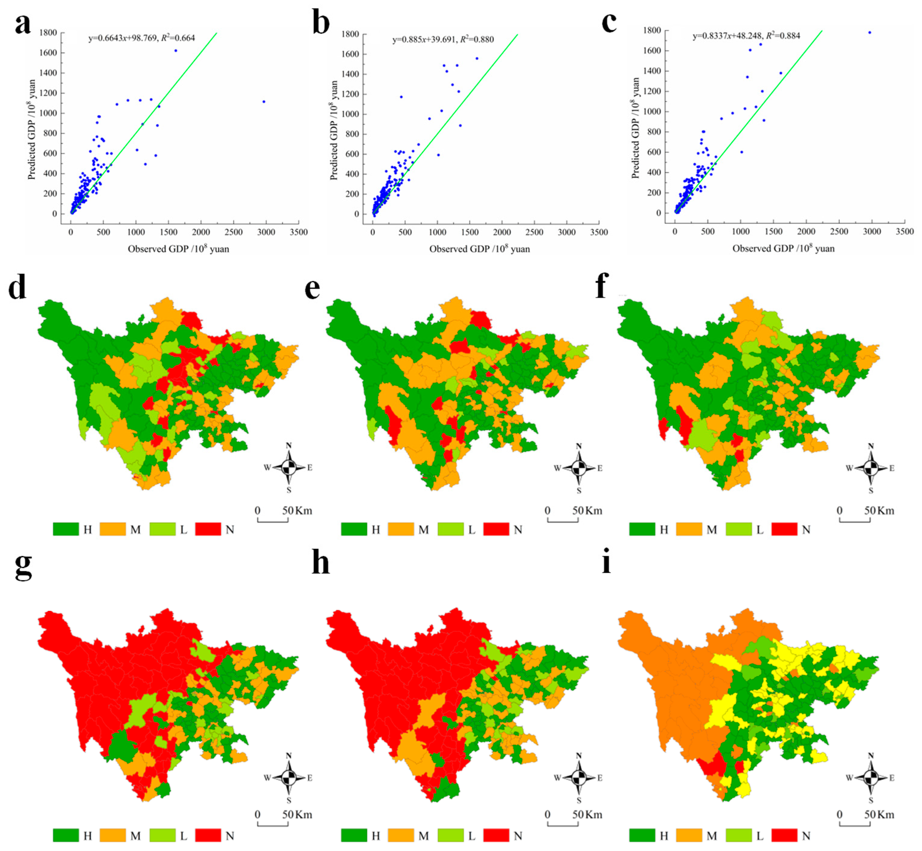
This study makes four contributions: (1) It develops a multisource, county-level GDP spatialization framework for a complex mountainous province, integrating corrected NPP/VIIRS NTL with POIs, land-use structure, terrain, climate, accessibility and population density within a unified GWR-based modeling scheme, and demonstrates that this spatially adaptive, multisource approach substantially outperforms both NTL-only models and the global OLS specification—confirming that spatial nonstationarity is an intrinsic feature of the GDP–proxy relationship in Sichuan. (2) It quantifies the marginal contribution of each supplementary data source within the GWR framework: adding POIs raises the R2 from 0.662 to 0.837, and further incorporating PFL raises it to 0.882, demonstrating that enriching the indicator system with functionally complementary proxies is the primary pathway to improved estimation accuracy in heterogeneous landscapes. (3) It characterizes the county-level economic geography of Sichuan, portraying a clear basin–plateau gradient, identifying high–high and low–low spatial clusters associated with a core–periphery structure, and mapping the development corridors that connect the Chengdu Plain to secondary urban centers. (4) By mapping GWR coefficient surfaces for terrain, precipitation, accessibility, population density and construction land, it translates statistical estimation into location-specific development diagnostics, providing a direct empirical basis for differentiated territorial planning recommendations across the diverse county types of mountainous Sichuan.
2. Materials and Methods
2.1. Study Area: Sichuan Province
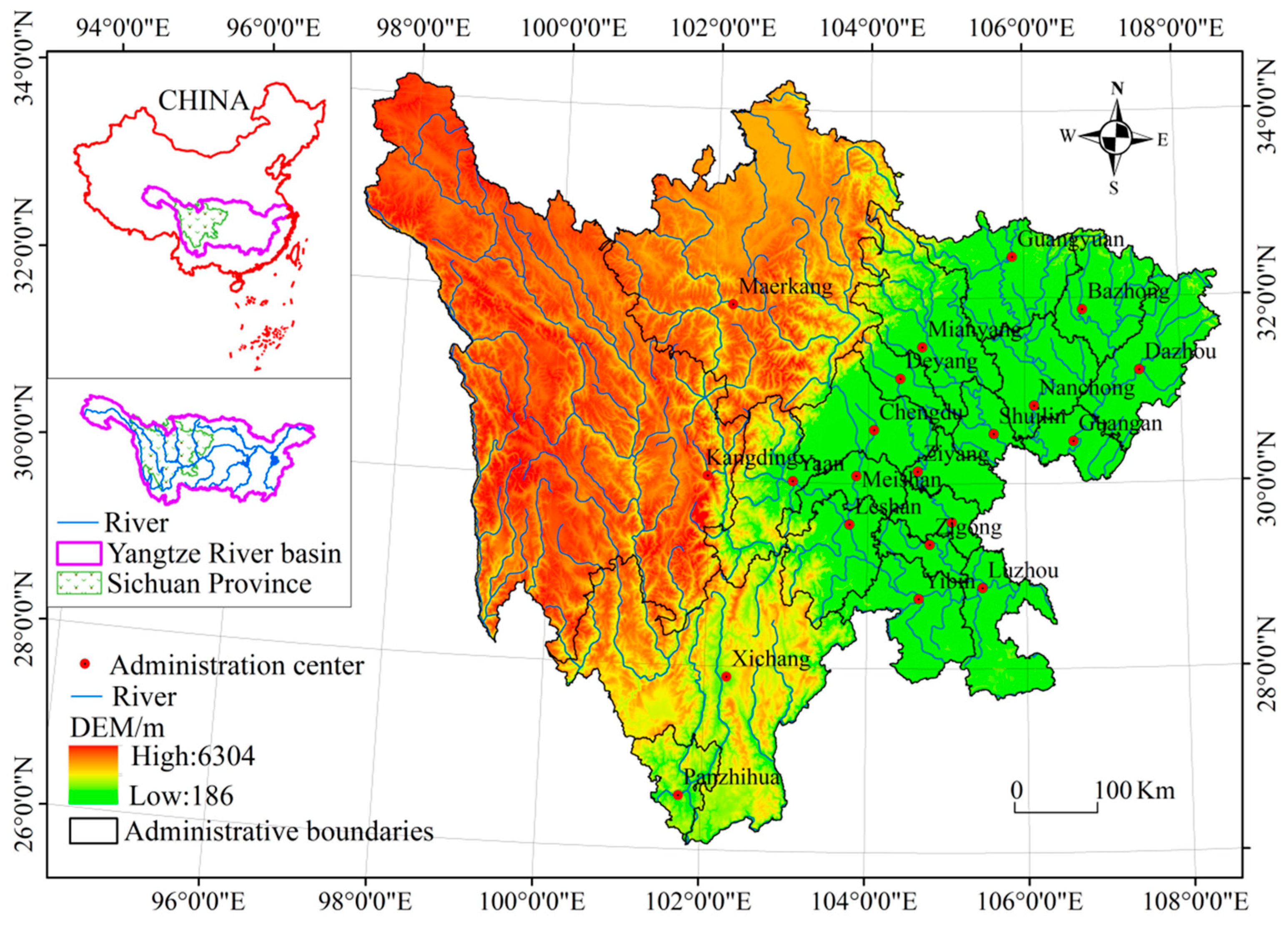
Sichuan Province is in southwestern China, in the upper part of the Yangtze River basin, with a total area of about 4.86 × 10
5 km
2 (
Figure 1). The geographic extent, coordinate boundaries, administrative centers and river network are shown in
Figure 1. The province is in a clear transition zone between the Qinghai–Xizang Plateau to the west and the middle and lower Yangtze River Plain to the east. Its terrain varies greatly, with elevations generally dropping from west to east and a height difference of about 7300 m. Western and northwestern Sichuan are mainly composed of high mountains and plateaus with rough terrain and few settlements, while the Sichuan Basin in the central part and the low hills in the east have relatively flat terrain and dense river and transport networks [
26].
Sichuan’s climate shows clear regional and vertical differences, shaped by the strong influence of the terrain. The western mountainous plateau is cold–temperate, where the average annual temperatures are around 4–12 °C and the annual precipitation is between 500 and 900 mm. By contrast, the eastern basin has a subtropical monsoon climate, with an average annual temperature of around 16–18 °C and an annual precipitation of 1000–1300 mm. It has produced a great variety of natural settings and land uses, including intensively cultivated alluvial plains, wooded mountains, and alpine meadows [
27].
This ecological diversity has a close relationship with a well-defined core–periphery structure in the regional economy. Most of the population, transport facilities, and high-value industries are found in the middle of the province, on Chengdu Plain, whereas many outer mountainous and plateau counties rely more heavily on agriculture, resource extraction, and tourism and have prolonged constraints on their accessibility and degree of development. The combination of highly urbanized basins and thinly populated highlands within a single province makes Sichuan a representative test case for county-level GDP spatialization with multisource spatially adaptive models. Specifically, its 183 counties span an elevation range exceeding 7000 m and have a GDP per capita ratio of more than 10:1 between the richest and poorest counties and land-use compositions ranging from nearly 100% cropland to nearly 100% alpine meadow, providing sufficient internal variance to evaluate model performance across a wide spectrum of geographic and economic conditions.
2.2. Data Sources and Preprocessing
In order to record the economic activity and the natural and human factors behind it, this paper integrates several remote sensing, geospatial and statistical information datasets. The primary data are NPP VIIRS nighttime-light images, digital elevation models (DEMs), gridded climate data (temperature and precipitation), POIs, land-use data, accessibility measures based on distance, population and industrial structure statistics, and county-level GDPs and administrative boundaries. Every spatial dataset was converted into WGS_1984 projection coordinates or GCS_WGS_1984 geographic coordinates and rescaled to a uniform spatial resolution in order to maintain geometric consistency. Administrative units at the county level were taken as the elementary spatial units in the model construction and assessment.
Artificial lighting and human activity density were characterized using the annual composite NPP/VIIRS day/night band (DNB) nighttime-light imagery for the year 2020 [
9]. To make them more appropriate to economic analysis, the initial photographs were rectified by continuity correction, oversaturation correction and regression-based calibration, as per traditional procedures in the literature [
28]. The digital number (DN) values were modified in ENVI (version 5.6.3; L3Harris Geospatial, Broomfield, CO, USA)through Band Math, and only DN values between [−63 and 63] were retained, whereas those that were less than −63 or greater than 63 were deleted. The brightest isolated pixels were identified based on the maximum pixel value of Chengdu and discarded to minimize blooming and sensor noise. The finally corrected NTL images could thereby be better aligned to the stable surface lighting patterns and confidently aggregated at the county level to create indicators.
DEM data of the US Geological Survey (USGS) and gridded climate data of the Resource and Environmental Science and Data Center of the Chinese Academy of Sciences were used to display the terrain and climate conditions and calculate the mean elevation by county to represent the terrain conditions and how they restrict the development of settlements and infrastructure. Temperature grids and precipitation grids were processed to obtain the county-wise average annual precipitation, which demonstrates water and climatic conditions that influence agricultural productivity and development constraints.
The intensity of human activity and functional structure were also recorded in the form of POI and accessibility information. The POIs were obtained via the Gaode (Amap; AutoNavi Software Co., Ltd., Beijing, China;
https://lbs.amap.com/) platform with its web API in Python (version 3.8; Python Software Foundation,
https://www.python.org/) and contain most types of services that are commercial, industrial, and governmental, as well as transport facilities. All POI counts were summed up per county, after deleting duplicate and non-valid records, and converted into density indicators, which indicate the number and variety of socio-economic activities. The average distances between the cells of the grids and their corresponding county seats were used as an indicator of accessibility and calculated in a GIS setting with the Euclidean distance, which was subsequently aggregated to the county level. This distance measurement indicates how difficult it is to get to administrative and economic centers and is particularly crucial in a province with high-terrain obstacles [
29].
Population and economic statistics were obtained from the Sichuan Statistical Yearbook for 2020 (Sichuan Provincial Bureau of Statistics, 2021). The data include county-level GDP, population density, and sectoral shares of primary and secondary industries. The population density gives information about the demographic pressure and market size, whereas the industrial structure variables give the relative significance of agriculture and manufacturing in the economies of different counties. The dependent variable used in the model construction and subsequently to test the validity of the results of spatialization was the county-level GDP.
The county-level administrative boundaries were based on the National Basic Geographic Information Center (NBGIC) scale of 1:1,000,000. They formed the spatial reference for combining all the raster and point-based indicators and for mapping the results of the models. After preprocessing, each county had a consistent set of indicators from the multisource data, forming the basis for the following regression modeling and spatial analysis.
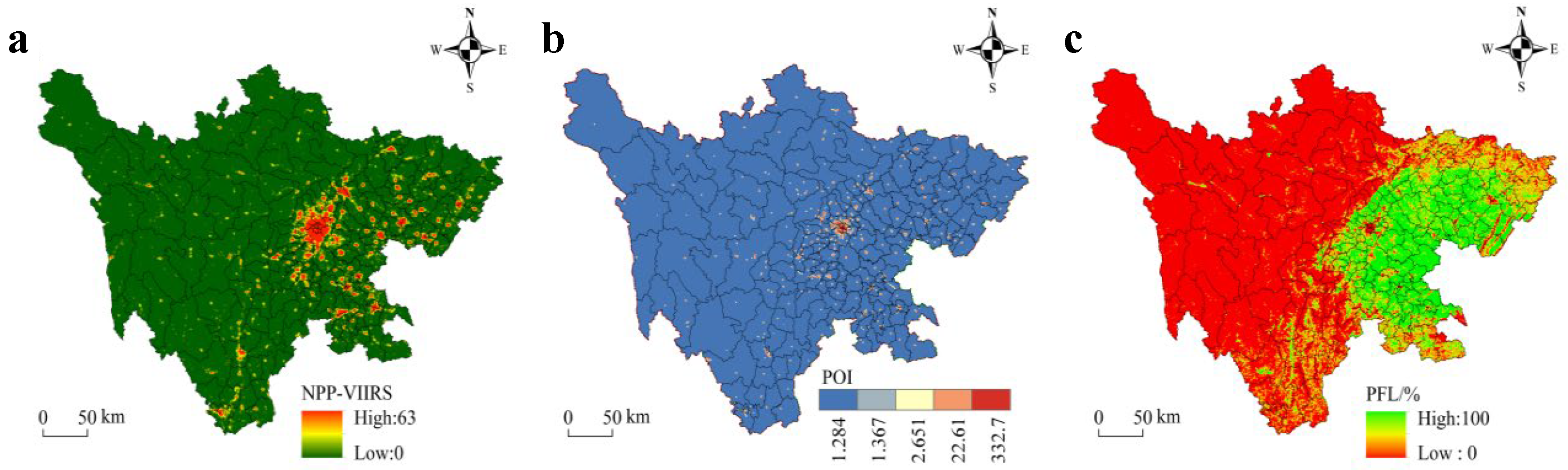
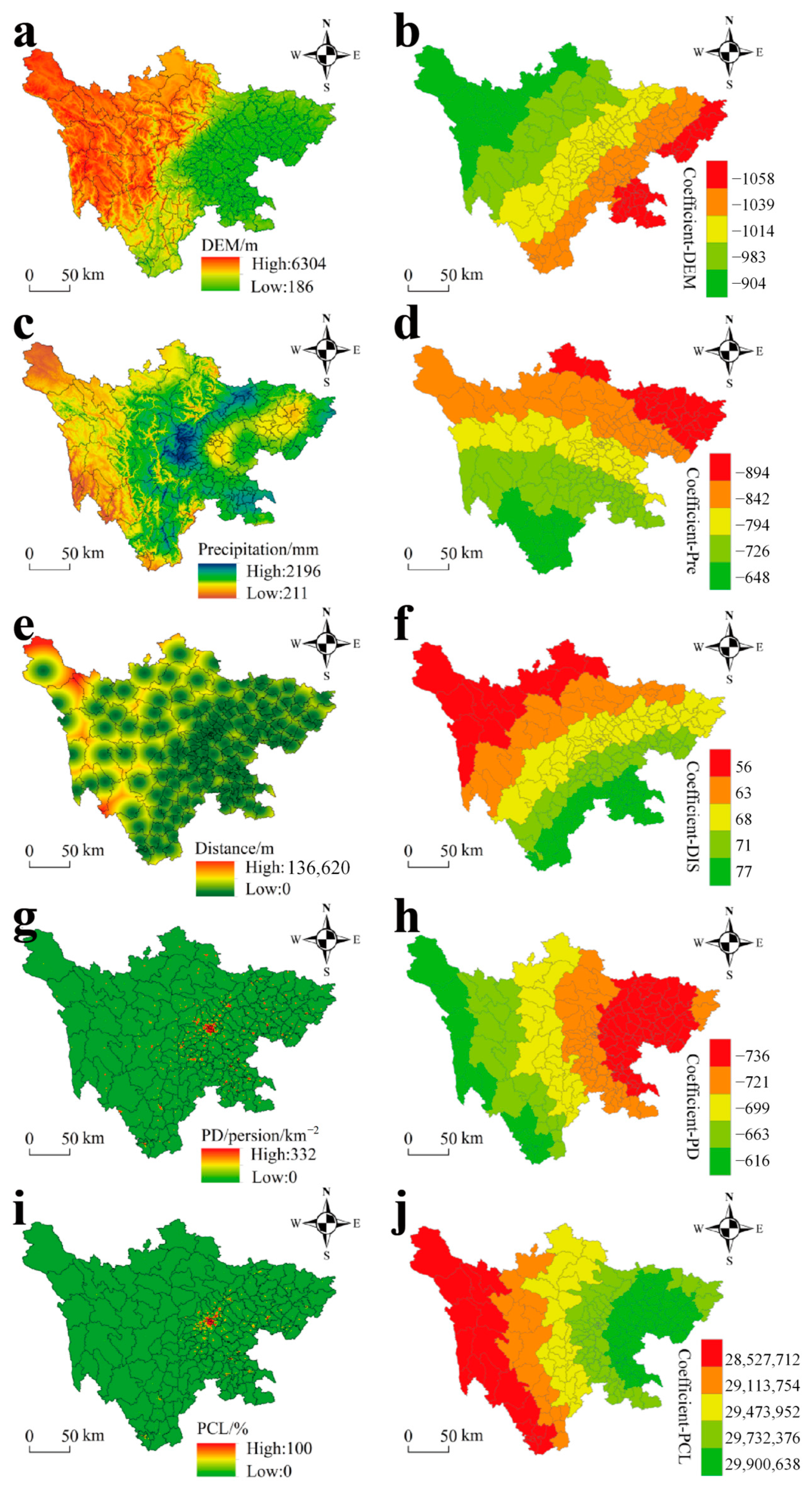
Figure 2 shows the spatial patterns of several main explanatory variables, including the corrected NPP–VIIRS nighttime lights, POI density, and proportion of farmland, and highlights the difference between the highly urbanized Chengdu Plain and the surrounding mountainous and plateau regions.
2.3. Variable Selection and Indicator Construction
On the basis of the processed datasets, a unified county-level indicator system was constructed for GDP spatialization. The statistical county-level GDP serves as the response variable, while a set of NTL-based socio-economic and environmental indicators are used as explanatory variables. From the corrected nighttime-light imagery, four commonly used indicators proposed by Zhao et al. [
30] are computed: the total nighttime-light intensity, the average light intensity, the ratio of lit area to total county area, and a composite nighttime-light index that combines information on intensity and spatial extent. Together, these indicators characterize both the magnitude and distribution of artificial lighting within each county and thus provide a first-order proxy for overall economic activity.
To complement the nighttime-light information and better represent the determinants of county-level GDP, additional variables are derived from POI, land-use, topography, climate, accessibility and population data. The POI density reflects the concentration and functional diversity of socio-economic activities and is expected to be positively associated with the GDP. The land-use structure is described by the proportion of farmland (PFL) and the proportion of construction land (PCL), which represent, respectively, the agricultural land endowment and built-up development intensity. The mean elevation derived from the DEM and mean annual precipitation capture terrain and hydroclimatic constraints on development. Accessibility is measured in terms of the mean distance to the county seat, which can be used as an approximation of the accessibility of administrative and economic centers, whereas population density measures the size and concentration of the population living there, and therefore their possible labor and market capacity.
Descriptive statistics and correlation tests were performed on all candidate indicators prior to inclusion in the regression models. Candidate variables with VIFs exceeding 10 were removed to avoid severe multicollinearity. Two variables—population density (PD) (VIF = 7.03) and proportion of construction land (PCL) (VIF = 8.83)—exhibited moderate collinearity but were retained because they represent conceptually distinct dimensions (demographic pressure vs. built-environment intensity). The robustness checks presented in
Section 3.3.1 confirm that the main findings are insensitive to their joint inclusion. The other variables were standardized in order to eliminate the influence of varied units and scales. The final explanatory variables selected in the comparative OLS and GWR models comprise NTL-based indicators, POI density, PFL, PCL, mean elevation, mean annual precipitation, distance to county seat, and population density. Such a multisource indicator system provides a comprehensive view of the intensity of human activity, the structure of land use, and environmental and accessibility constraints, which are collectively responsible for the spatial pattern of the county-level GDP in Sichuan.
2.4. Overall Framework of Multisource Spatial Regression Approach
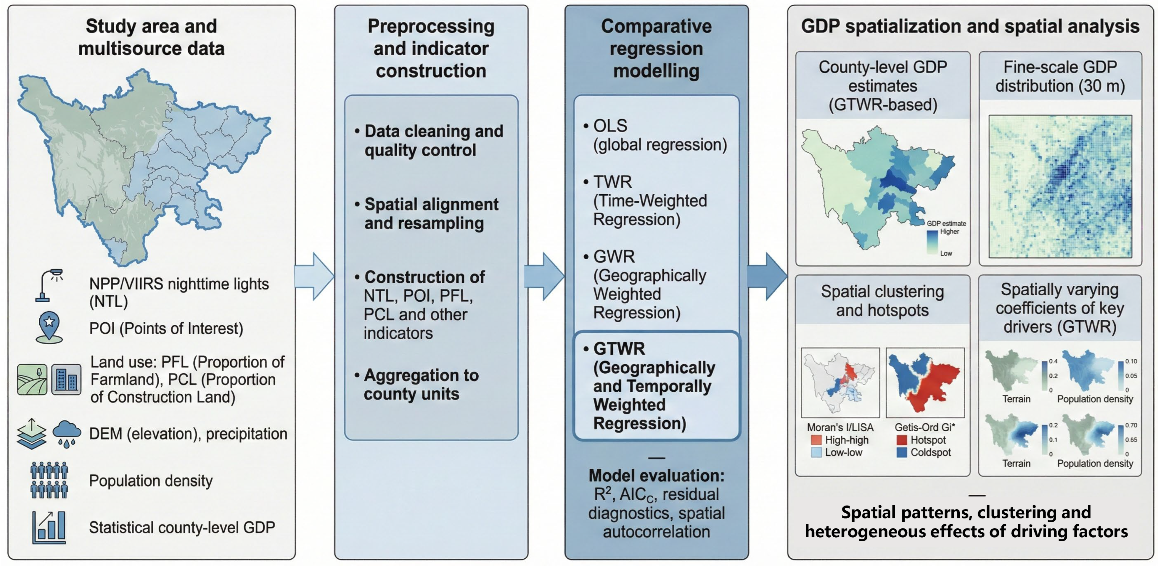
The methodological framework of this study follows four main stages: (i) preprocessing and harmonization of multisource data, (ii) construction of county-level indicators, (iii) comparative regression modeling with global and spatially adaptive specifications, and (iv) spatialization and spatial analysis of GDP (
Figure 3). All spatial datasets were projected to a common geographic coordinate system and resampled to a unified spatial resolution. County-level administrative units were used as the basic analysis units, and all raster and point-based data were aggregated accordingly.
Socio-economic intensity was first represented by indicators derived from the corrected NPP–VIIRS nighttime-light data. Based on commonly used indicators in the nighttime-light literature, four indices were calculated from the corrected NPP–VIIRS imagery: the total nighttime-light intensity (TNL), the light area ratio (S), the average light intensity (I), and a composite nighttime-light index (L) that combines information on intensity and spatial extent [
30]. These indices are computed from the gray-level values of light pixels according to Equations (1)–(4):
where
and
denote the gray-level value and number of pixels in class
, respectively;
is the maximum gray-level value;
is the total number of light pixels in the administrative unit;
is the area of all light pixels;
is the total area of the administrative unit;
and
are the weights of the average intensity and light area ratio, respectively. Together, these indicators capture both the magnitude and spatial extent of the nighttime lighting within each county.
In parallel, auxiliary variables describing land-use structure, environmental conditions, accessibility and population were constructed from POI, land-use, DEM, climate, distance and population datasets, as detailed in
Section 2. These variables, together with the NTL-derived indices, form a unified county-level indicator system that serves as the input to the regression models. The core of the framework is a comparative modeling scheme that estimates county-level GDP using two types of models: Ordinary Least Squares (OLS) as a global benchmark and Geographically Weighted Regression (GWR) as the primary spatially adaptive model. Their performances are compared under three progressively enriched variable configurations—NTL only, NTL+POI, and NTL+POI+PFL—to isolate the marginal contribution of each additional data source. Finally, the GWR model calibrated on the full multisource indicator set is used to derive spatialized GDP estimates, and spatial autocorrelation and hotspot analyses are applied to characterize the resulting GDP surface and its driving-factor patterns [
31].
2.5. Regression Models: OLS and GWR
To examine the effects of spatial nonstationarity on county-level GDP estimation, two regression models with contrasting structural assumptions are employed. Both models use county-level GDP as the dependent variable and the multisource indicators described in
Section 2.3 as explanatory variables.
The OLS model provides a global benchmark under the assumption that the relationship between GDP and its predictors is spatially invariant. OLS estimates a single set of coefficients by minimizing the sum of squared residuals:
where
is the observed county-level GDP for county
is the vector of explanatory variables;
is the vector of regression coefficients;
is the matrix of explanatory variables across all n counties; and
y is the vector of dependent variable observations. Because OLS assumes spatial invariance, its residuals may exhibit spatial autocorrelation in heterogeneous settings; a significant Moran’s I statistic on OLS residuals would confirm the presence of spatial nonstationarity that OLS cannot accommodate.
GWR extends OLS by allowing regression coefficients to vary continuously across space. For each county i with geographic centroid coordinates (
ui,
vi), the local regression equation takes the following form:
where
β0(
ui,
vi) is a location-specific intercept and
βₖ(
ui,
vi) are location-specific slope coefficients. Nearby counties receive larger weights in the local estimation, and the weight for county
j when estimating coefficients at location
i is assigned using an adaptive Gaussian spatial kernel:
where
dij is the Euclidean distance between the centroids of counties
i and
j, and
hS is the spatial bandwidth. The local coefficient vector at each location is estimated as:
where W(
ui,
vi) is the diagonal spatial weight matrix. The spatial bandwidth (
hS) is selected by minimizing the corrected Akaike information criterion (AICc), which penalizes added complexity and guards against over-fitting. GWR is particularly appropriate for county-level GDP spatialization in Sichuan because it minimizes residual spatial clustering, improves prediction accuracy in topographically heterogeneous areas, and simultaneously produces interpretable coefficient surfaces that reveal how the effects of each driving factor vary across the basin–plateau gradient [
23].
Because the present analysis is based on a single-year cross section (2020), temporally weighted extensions (e.g., GTWR) are inapplicable: all observations share an identical time stamp, so any temporal kernel degenerates to a constant. Multi-year extension using geographically weighted panel regression (GWPR) is discussed in
Section 4.4.
2.6. Model Calibration and Evaluation
GDP is used as the dependent variable in all models, while NTL-derived indices, land-use structure, environmental conditions, accessibility and population density serve as explanatory variables. Before model calibration, multicollinearity among the explanatory variables is examined using correlation analysis and variance inflation factors in SPSS (version 26.0; IBM Corp., Armonk, NY, USA). Variables with unacceptable collinearity are removed or combined, and the remaining indicators are standardized to remove unit effects.
Data–model correspondence. Both models are calibrated on county-level cross-sectional data for the year 2020 (
n = 183 counties).
Table 1 summarizes the temporal coverage and resolution of each variable: GDP, NTL, POI density, PFL, PCL and precipitation are observed for 2020; DEM and accessibility (DIS) are time-invariant. No multi-year panel is constructed, and no variable is recalculated for additional years. Both OLS and GWR are estimated directly on the 2020 cross section. As noted in
Section 2.5, temporally weighted extensions are inapplicable to this single-year design.
To address the research questions, several model–data combinations are calibrated. First, NTL-only specifications are estimated using OLS and GWR to evaluate the baseline performance of nighttime lights as a single proxy. Second, multisource models that include NTL, POI density, PFL, PCL, elevation, precipitation, distance to county seat and population density are estimated using the same two regression approaches.
Model performance is evaluated using a set of complementary statistics, including the coefficient of determination (
), adjusted
, residual sum of squares (RSS) and AICc [
8]. Residual diagnostics are carried out to test the presence of heteroscedasticity and non-normality. In order to evaluate spatial behavior, the global Moran’s I is calculated based on the residuals of a model, and a decrease in residual spatial autocorrelation means that the model has a greater ability to explain spatial structure. The highest-ranking model in the sense of goodness-of-fit and residual properties is used subsequently used to produce county-level GDP estimates and fine-scale spatialization outcomes to be analyzed spatially.
2.7. Spatial Autocorrelation and Hotspot Analysis
Both global and local spatial autocorrelation statistics are used to describe the spatial pattern of the county-level GDP and provide a validation of the spatial structure of model outputs. Global autocorrelation is assessed using Moran’s I, which measures the overall similarity of GDP values among neighboring counties. The statistic is calculated as
where
is the number of counties;
and
are the observed GDP values in counties
and
;
is the mean GDP;
is the element of the spatial weight matrix describing the contiguity between counties
and
; and
. Positive values of Moran’s I indicate positive spatial autocorrelation (high–high or low–low clustering), negative values indicate negative autocorrelation (high–low or low–high patterns), and values close to zero suggest randomness.
Local spatial autocorrelation is examined using Anselin’s Local Moran’s I, which identifies specific clusters and outliers of GDP. The local statistic for county
is given by
where
is the GDP of county
;
is the mean GDP;
is the spatial weight between counties
and
; and
is the variance in GDP. Local Moran’s I allows for the identification of statistically significant high–high, low–low, high–low and low–high clusters.
To further detect and map hotspots and coldspots of GDP, Getis–Ord (
) statistics are calculated. This local indicator evaluates whether high or low GDP values are spatially clustered around each county. The statistic is expressed as
where
is the GDP value for county
, nnn is the total number of counties, and
denotes the spatial weight between counties
and
within a specified distance threshold (
) (typically 1 for neighbors and 0 otherwise). The resulting
-scores and
-values are used to identify statistically significant hotspots (high-GDP clusters) and coldspots (low-GDP clusters).
Together, the global Moran’s I, Local Moran’s I and Getis–Ord statistics provide a comprehensive assessment of the spatial organization of the county-level GDP in Sichuan, supporting the analysis of spatial gradients and clustering patterns and the evaluation of different modeling strategies.
4. Discussion
4.1. Methodological Implications of Multisource Spatial Regression Framework
The results demonstrate that combining multisource geo-big data with spatially adaptive regression provides clear and substantial methodological advantages for county-level GDP spatialization in complex mountainous regions. The transition from global OLS to locally weighted GWR yielded consistent improvements in the goodness of fit and information criteria across all variable configurations, confirming that spatial nonstationarity is an intrinsic structural feature of the GDP–proxy relationship in Sichuan rather than a statistical artefact. The decline in the residual Moran’s I from OLS to GWR further confirms that this nonstationarity is genuine and pervasive: the global model systematically misestimates GDP in topographically extreme counties because it cannot adapt its coefficients to the local geographic and economic context. This finding is consistent with Huang et al. [
17], who documented significant spatial nonstationarity in county-level economic drivers across multiple Chinese provinces using a multiscale GWR approach, and with the broader GWR literature demonstrating that spatially adaptive estimation is indispensable wherever the relationship between economic outcomes and their predictors varies with geographic context. For Sichuan specifically, the sources of spatial nonstationarity are rooted in persistent structural contrasts—terrain, accessibility, agglomeration economies and industrial composition—that differ fundamentally between the Chengdu Plain core and the surrounding highlands. These structures change slowly over time; their spatial differentiation, rather than temporal dynamics, is therefore the appropriate target of the modeling framework adopted here.
Second, the integration of NTL with POIs and land-use structure substantially mitigates well-known weaknesses of nighttime-light-only approaches. The strong correlation between TNL and GDP at the provincial scale is consistent with previous research, but the decline in the performance of NTL-only models in high-altitude and underdeveloped counties illustrates the scale dependence and contextual sensitivity of the NTL–economy linkage. Density of POIs provides more information about the functional intensity and variety of economic activities, and PFL and PCL reflect the underlying land-use structure that limits production and settlement. Explanatory variance improves significantly and spatial error clustering in western Sichuan decreases when these variables are integrated into the GWR framework, indicating that multisource integration is essential for attaining reliable estimates in heterogeneous landscapes.
These findings are broadly consistent with, and extend, the existing literature on multisource GDP spatialization. Li et al. [
11] conducted national-scale GDP spatialization in China using NPP/VIIRS data from 2013 to 2023, although their study employed a global regression that could not account for local heterogeneity. Ustaoglu et al. [
34] combined NTL with MODIS vegetation indices for GDP estimation in Turkey and similarly found that multisource models outperformed NTL-only specifications, though their reported R
2 values (approximately 0.70–0.75) were lower than those achieved here, likely because their study region exhibited less extreme topographic heterogeneity. Chen et al. [
14] integrated NTL with street-view imagery and POIs for GDP estimation in Dongguan and achieved comparable accuracy, but their urban-dominated study area reduced the need for spatially varying coefficients. Compared with these studies, the present work demonstrates that the GWR framework is particularly advantageous in mountainous settings where the GDP–proxy relationship varies markedly between basin cores and highland peripheries. The superiority of GWR over OLS observed here (R
2 improvement from 0.801 to 0.882) is also consistent with Huang et al. [
17], who identified significant spatial nonstationarity in county-level economic drivers across multiple Chinese provinces using a multiscale GWR approach.
The individual contributions of the supplementary proxies differ markedly and carry substantive implications for indicator design. POI density is by far the most consequential addition: its inclusion raises the GWR R
2 from 0.662 to 0.837, an increment of 0.175 that reflects the strong alignment between service facility density and urban economic output. This result is consistent with Chen et al. [
14], who similarly found that POI information substantially improved the GDP estimation accuracy in Dongguan by capturing the functional intensity of economic activities that nighttime lights alone cannot differentiate. The further inclusion of PFL raises the GWR R
2 from 0.837 to 0.882 (+0.045), a more modest but meaningful gain concentrated in the agricultural counties of the eastern hills and the basin periphery. This asymmetry reflects Sichuan’s current economic structure, in which service and industrial activities—well captured by POIs—dominate provincial GDP, while farmland proportion plays a secondary and spatially concentrated explanatory role. Nonetheless, PFL is retained in the final specification on both empirical and theoretical grounds: empirically, its inclusion reduces residual spatial autocorrelation in agricultural counties; theoretically, in provinces or regions where primary-sector value added constitutes a larger GDP share, farmland proportion is expected to carry greater explanatory weight, and its omission could introduce systematic bias. We recommend that PFL be evaluated as a standard candidate variable in any application of this framework, with its marginal contribution assessed empirically in each regional context.
Third, through the estimation of spatially varying coefficients, GWR converts GDP spatialization from a purely predictive task into an analytical method for comprehending development mechanisms. The coefficient surfaces for elevation, precipitation, distance, population density and construction land go beyond simple correlation and provide locality-based elasticities that are interpretable in terms of physical constraints, infrastructure networks and demographic processes. This represents a significant improvement over purely statistical or machine learning methods that may achieve comparable predictive accuracies but offer limited transparency for policy-related interpretation. These findings lend credence to the idea that spatially adaptive and interpretable models are especially appropriate for applied regional studies with the ultimate aim of informing place-based development policies.
4.2. Economic–Geographical Interpretation of County-Level GDP Patterns in Sichuan
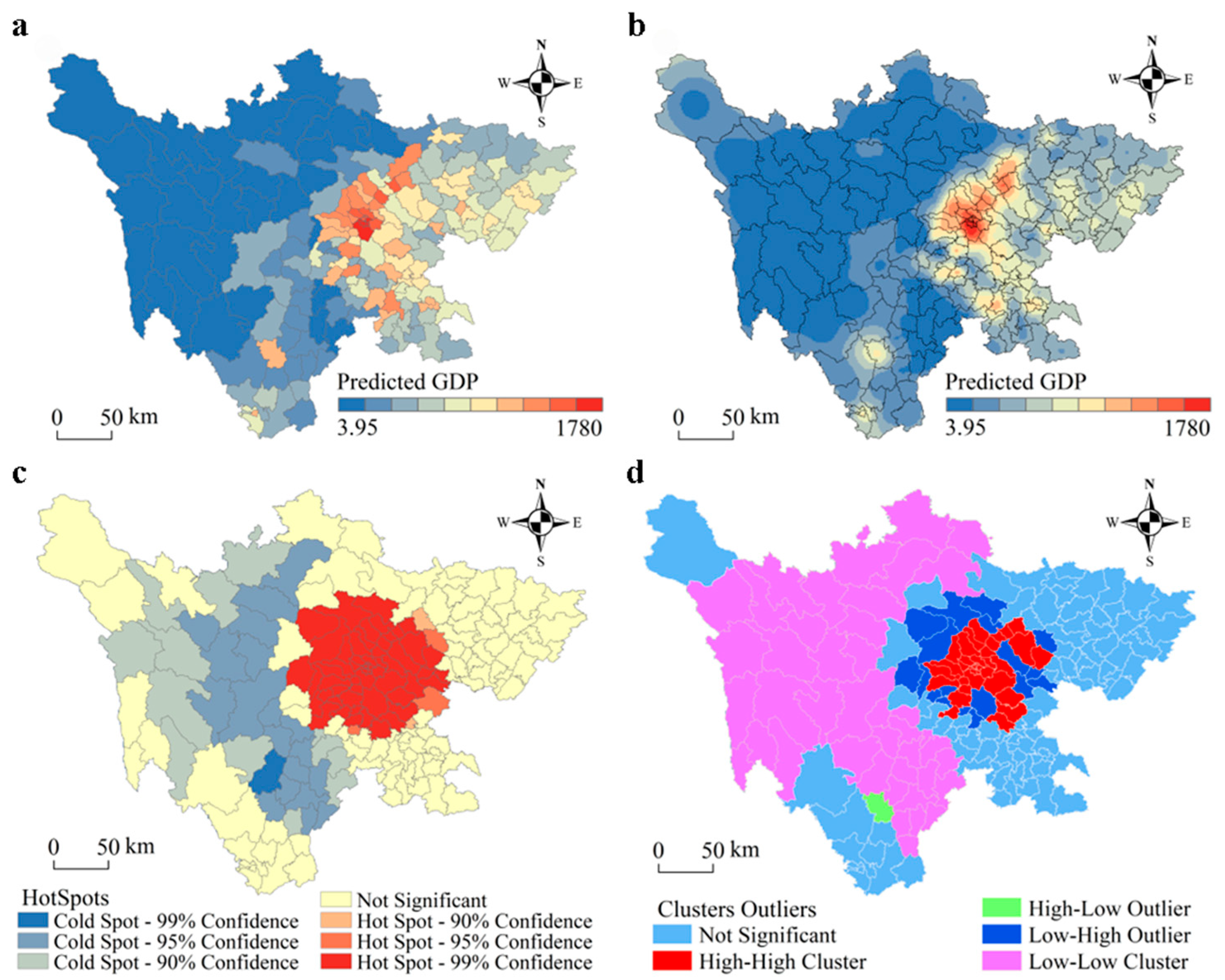
The analysis of the GDP surface and associated spatial diagnostics based on the GWR model sheds light on the economic geography of Sichuan. At the provincial level, the steep basin plateau gradient and the presence of high values within and around the Chengdu Plain are characteristics of a typical core–periphery pattern. There is a strong coincidence between high–high clusters and hotspots and the area of the Chengdu metropolitan region, as well as neighboring industrial and service hubs, where the positive topography, high-density transport infrastructure, and diverse industrial base enhance the tendency to agglomerate. On the fine-scale GDP map, it can be seen that such cores follow large corridors, which means that transport-led corridor development plays a significant role in the formation of the regional economy.
However, in contrast, low–low clusters and coldspots in the northwestern plateau and some parts of the Panxi area are associated with regions of high altitudes, rough topographies, low populations, and poor accessibility. Negative coefficients of elevation and precipitation are the highest here, and positive ones of construction land are weakened, which suggests that the environmental constraints and hazard exposure prevail over the benefits of agglomeration. The fact that there are high–low and low–high outliers, such as Xichang and a few counties on the edges of the basin, is a sign of a transitional space where local comparative advantages (e.g., energy resources, tourism or specialized agriculture) can produce higher levels of GDP despite the overall unfavorable environment, or vice versa, where structural vulnerabilities remain near the center of wealth.
The spatial heterogeneity of the coefficient surfaces offers a more subtle explanation of these patterns. Construction land has significant positive coefficients in the basin core and most eastern hill counties, but elevation has a rather weak negative effect. The implications of this combination are that urbanization, industrialization, and infrastructure spending remain potent sources of economic growth. Conversely, in the western highlands, the identical growth in construction land produces less GDP, and the negative impacts of elevation and precipitation predominate; in such a context, traditional approaches to urbanization-driven policy will not bring about the same returns. There are negative marginal effects of population density in densely populated areas, which indicates possible congestion, environmental factors, and a lack of investment in human capital, whereas in thinly populated plateau areas, the additional population has little direct effect on the GDP, since other limitations hold. Overall, the GWR findings complement and refine the core–periphery and corridor development perspectives by measuring how physical geography and human systems combine to form different development paths across counties.
The core–periphery pattern observed in Sichuan echoes findings in other developing mountainous regions. Han et al. [
24] documented a similar spatial dichotomy in the Chengdu–Chongqing economic circle, where basin-centered agglomeration coexists with persistent peripheral underdevelopment. Zhang et al. [
25] identified analogous impacts of urban expansion on the green land efficiency in the same urban agglomeration, reinforcing the finding that construction land effects are spatially contingent. The negative marginal effects of population density in densely populated basins observed in the present study are consistent with congestion-related productivity losses reported for rapidly urbanizing Chinese cities [
35]. Internationally, the challenges of NTL-based GDP estimation in mountainous terrains documented here parallel those reported by McCord and Rodriguez-Heredia [
7] for rural Paraguay, where NTL similarly failed to capture non-luminous economic activities, suggesting that the multisource GWR framework may be transferable to comparable settings beyond China.
The GWR coefficient surfaces also reveal important within-county-type variation that enriches the economic–geographical interpretation. Among the high–high cluster counties concentrated on the Chengdu Plain, the positive PCL coefficients are the largest in the inner metropolitan districts of Chengdu, Mianyang and Leshan, where construction land expansion is associated with industrial upgrading, logistics development and tertiary-sector agglomeration. These counties also exhibit the most strongly negative population density coefficients, suggesting that the productivity gains of agglomeration are being partially offset by congestion costs—a pattern consistent with the diminishing returns to urban density documented for rapidly growing Chinese cities [
35]. This finding implies that the continued physical expansion of construction land in basin core counties may yield progressively smaller GDP increments unless accompanied by improvements in urban management quality and human capital investment.
In the transitional hill counties of eastern Sichuan—classified as neither hotspots nor coldspots in the Getis–Ord Gi* analysis—the PCL coefficients remain positive but are substantially smaller than those in the basin core, and the DIS coefficients are among the highest in the province. This combination suggests that improved connectivity to county seats is currently the binding constraint on economic development in these areas: once accessibility is secured, additional construction land begins to yield meaningful GDP returns. This pattern supports the hypothesis that transport-led corridor development is the primary mechanism linking secondary urban centers to the growth dynamics of the Chengdu Plain, consistent with the corridor development perspective advanced by Han et al. [
24].
Among the low–low cluster counties of the western plateau, the DEM and Pre coefficients are the most strongly negative, while the PCL coefficients are the weakest. This configuration indicates that environmental constraints—extreme elevation and precipitation-related hazard exposure—impose binding limits on economic productivity that physical infrastructure expansion alone cannot overcome. Economic development in these counties is therefore contingent on reducing environmental vulnerability, which encompasses both engineering solutions, such as slope stabilization and flood control, and policy measures, including diversification toward eco-tourism, traditional crafts and high-value specialty agriculture. The spatially explicit GWR framework makes it possible to identify precisely which counties face these compounded constraints, enabling policymakers to target interventions at the right places rather than applying uniform provincial policies that work well in the basin but are ineffective or counterproductive in the highlands.
4.3. Policy Implications for Mountainous Regional Development and Spatial Planning
The multisource GWR framework generates three distinct categories of policy-relevant insight that correspond directly to the three county typologies identified by the spatial analysis.
For basin core counties—the high–high clusters and hotspot zones concentrated on the Chengdu Plain and adjacent metropolitan corridors—the dominant policy challenge is managing the transition from extensive to intensive growth. The GWR coefficient surfaces show that construction land retains a strong positive effect on GDP in these counties, but that population density coefficients are increasingly negative, a signature of congestion costs that partially offset agglomeration gains. Policy should therefore prioritize: first, the qualitative upgrading of the existing construction land through redevelopment of underutilized industrial land for higher-value uses, densification of existing urban areas, and investment in public transit to reduce intra-metropolitan congestion; second, selective strengthening of inter-city transport corridors to distribute growth pressure toward secondary centers, such as Mianyang, Leshan and Zigong, preventing over-concentration in Chengdu; and third, environmental carrying-capacity assessment integrated into land-use zoning decisions, since rapid built-up expansion in the basin increases impervious surface cover, reduces flood buffering and elevates the urban heat risk. The Chengdu metropolitan area is likely to remain the primary strategic growth pole of Sichuan; managing its expansion proactively is therefore a provincial priority rather than a purely local concern.
For transitional hill counties—the mixed or non-significant cluster zones in the northeastern, southeastern and southern hill areas—the binding constraints identified by GWR are accessibility deficits and moderate construction land endowments. The positive and spatially large DIS coefficients in these counties indicate that improving road connectivity to county seats would unlock latent economic potential by integrating local labor and product markets into the broader provincial economy. Policy priorities for this zone should include: first, targeted transport investment in county-to-county road upgrading and expressway spur connections, with cost–benefit analysis anchored to the locally estimated GWR elasticities; second, designation of small and medium-sized city development zones at strategic transport nodes, supported by industrial park incentives and logistics hub development; and third, preservation of farmland in areas where PFL coefficients indicate that primary-sector productivity remains a significant GDP contributor, balanced against the need for construction land to support small-scale urbanization. The hill zone is the most likely target for the managed decentralization of industrial and service functions from the Chengdu core, and the GWR coefficient evidence provides an empirical basis for prioritizing which counties and which transport connections would generate the highest economic returns from such decentralization.
For western plateau and high-mountain counties—the low–low clusters and coldspot zones in Ganzi, Ngawa and parts of Liangshan—the GWR coefficients confirm that environmental constraints, primarily elevation and precipitation-related hazard exposure, are the dominant limiting factors. Construction land expansion has the weakest positive effect in this zone and would impose high infrastructure costs relative to the GDP increment delivered. Population density effects are near zero, reflecting a demographic structure dominated by sparse and aging populations where additional labor supply alone does not translate into output growth. Effective policy for this zone must therefore address structural rather than cyclical constraints: accessibility investment should focus on resilient roads and digital connectivity rather than high-cost expressways, with particular attention to emergency access routes that reduce disaster-induced economic losses given the high coefficient magnitude on precipitation as a hazard proxy; eco-economy development—including protected-area ecosystem service payments, carbon offset schemes, high-value specialty agriculture, such as plateau medicinal herbs, yak products and high-altitude fruits, as well as nature-based tourism—represents a more environmentally sustainable and economically appropriate growth pathway than replication of basin-style industrialization; and inter-regional transfer payments and fiscal equalization mechanisms are essential to compensate these counties for their environmental stewardship functions and to ensure that residents in high-constraint areas have equitable access to public services regardless of limited local GDP.
Beyond these county-type-specific recommendations, the GWR framework also provides value at the monitoring and evaluation level. The spatially explicit GDP estimates and driving-factor coefficient surfaces can be updated as new annual NTL, POI and land-use data become available, enabling the continuous tracking of county-level economic change between official statistical releases. This near-real-time monitoring capacity is particularly valuable for detecting emerging spatial disparities—such as deteriorating accessibility coefficients following infrastructure damage events or rising population density coefficient magnitudes signaling congestion onset—that may require timely policy response. Integration of this spatially explicit economic information into land-use zoning, ecological red-line delineation and large-scale infrastructure project siting can help align economic growth trajectories with environmental carrying capacities, an alignment that is especially important in the sensitive mountain ecosystems of western Sichuan where economic activities and ecological functions are in close spatial proximity.
4.4. Limitations and Directions for Future Research
Although it has a number of strengths, this paper has various limitations that can be used to direct future work. First, even though the multisource data enhance representation of economic activities, every dataset has its own uncertainties. Non-economic lighting and sensor noise impact NTL; POI coverage relies on platform-specific recording behavior; the land-use and population datasets contain classification and estimation errors; and official GDP statistics have reporting and reconciliation problems. Such uncertainties spread throughout the modeling chain and can impact local estimates, particularly in counties with little data. The uncertainties could be quantified explicitly by future research, e.g., using error propagation analysis or Bayesian methods, and the advantages of adding other proxies (mobile phone data, freight flows or firm-level information when possible) could be investigated.
Second, the GWR model is flexible and interpretable but assumes a linear predictor–GDP relationship and employs a single-bandwidth structure per model. The non-linearities, threshold effects and interaction terms, such as the accessibility–construction land interaction or elevation–precipitation interaction, are not fully represented. Adding non-linear or hierarchical modeling methods or incorporating insights from the GWR coefficient surfaces into machine learning models could also improve predictive capabilities without losing interpretability. Also, the temporal aspect of this research is constrained by the availability and consistency of multi-year statistics at the county level. Because all variables are observed for a single year (2020), the present design captures spatial heterogeneity but not temporal dynamics. Extending the framework to multi-year panels using geographically weighted panel regression (GWPR) [
36] would enable analysis of temporal change within a spatially varying coefficient framework. Multi-year panel data would also enable the examination of dynamic phenomena, such as industrial restructuring, urbanization trajectories and policy shocks, which cannot be captured in a single cross section. Assembling a consistent county-level panel for Sichuan—reconciling boundary changes, statistical reclassifications and variable availability across years—is a priority for future work.
Third, the empirical analysis is confined to a single province. Although Sichuan encompasses a remarkably wide spectrum of terrain types (alluvial plains below 500 m, mid-altitude hills, alpine valleys above 3000 m, and high plateaus exceeding 4000 m), economic development levels (from the Chengdu megacity core to subsistence agriculture plateau counties), and land-use structures (intensive cropland, dense urban cores, alpine meadows), its internal diversity does not fully substitute for cross-regional validation. In particular, the NTL–GDP relationship may behave differently in coastal export-oriented economies, arid resource extraction regions, or densely industrialized deltas where light saturation and blooming patterns differ markedly from those in mountainous Sichuan. Systematic replication of the proposed framework in provinces with contrasting economic and physical geographies—such as Guangdong (coastal manufacturing), Guizhou (karst plateau, poverty), or Inner Mongolia (arid pastoral economy)—constitutes the most important direction for future work and is essential before the approach can be recommended for operational use beyond similar mountainous settings. Nevertheless, several design features of the framework are inherently transferable: the indicator system relies exclusively on globally or nationally available data sources (NPP/VIIRS, DEM, land-use maps, POI platforms, statistical yearbooks), the GWR estimation procedure is data-driven and does not require region-specific calibration beyond bandwidth optimization, and the comparative modeling protocol (OLS and GWR) can be applied without modification to any region where county-level GDP and geospatial covariates are available. These characteristics suggest that the framework is portable in principle, even though its empirical performance in other contexts remains to be demonstrated.
Conclusively, the present research is aimed at total GDP, and no differentiation has been made with regard to sectoral contribution or welfare-related measures. Information regarding the spatial distribution of per capita income, value added by sector, carbon emissions or ecosystem services would be very useful to answer numerous planning and sustainability questions. The extension of the multisource indicator system and the GWR modeling framework to these new dimensions could help with a better comprehension of the coupled human–environment system in mountainous areas.
All of these restrictions combined do not disprove the overall ideas but emphasize the opportunities to improve them. Further developments in the quality of data, methodological complexity, and applicability across regions will be critical in achieving the full potential of multisource, spatially adaptive GDP spatialization as a basis of evidence-based, regionally specific developmental strategies.
5. Conclusions
This study developed and evaluated a multisource GDP spatialization framework for Sichuan Province by integrating corrected NPP/VIIRS nighttime lights with POI, land-use structure, terrain, climate, accessibility and population indicators within a comparative modeling scheme comprising OLS as a global benchmark and GWR as the primary spatially adaptive model. The multisource GWR model achieves R2 = 0.882 (adjusted R2 = 0.872, AICc = 5712.26), substantially outperforming both the global OLS benchmark (R2 = 0.801) and NTL-only GWR baseline (R2 = 0.662), confirming that spatial nonstationarity is an intrinsic feature of the GDP–proxy relationship, and that enriching the indicator system with complementary geospatial proxies is the primary pathway to improved estimation accuracy.
Robustness checks—including models with population density (PD) and construction land proportion (PCL) excluded individually, and local VIF diagnostics computed across all 183 counties—verify that moderate collinearity between PD and PCL does not distort the main spatial patterns: coefficient signs, magnitudes and spatial distributions remain qualitatively unchanged in all reduced specifications, and local VIF values exceed 10 in only 26 of 183 counties concentrated in the Chengdu metropolitan core.
The GWR-based GDP surface reveals a pronounced basin–plateau gradient with high-value clusters concentrated in the Chengdu Plain and low-value zones extending across the western highlands (global Moran’s I = 0.33, p < 0.001). Spatially varying GWR coefficients reveal clear and interpretable regional differentiation: elevation and precipitation impose the strongest GDP constraints in high-altitude western counties; construction land exerts a consistently positive but spatially graded effect, strongest in the basin core and weakening toward the plateau; and accessibility and population density effects are context-dependent, shifting between growth-enabling and congestion-limiting roles depending on county type.
These coefficient patterns translate directly into three sets of differentiated policy recommendations. Basin core counties face an intensive-growth transition challenge and require managed expansion, congestion mitigation through public transit investment, and selective inter-city corridor development to distribute growth pressure toward secondary centers. Transitional hill counties are the most responsive to accessibility investment and targeted small-city industrialization at strategic transport nodes, where the GWR evidence indicates the highest expected returns to connectivity improvement. Plateau and high-mountain counties, where environmental constraints dominate over agglomeration effects, require accessibility-first, eco-economy and fiscal equalization strategies—particularly ecosystem service payments, specialty agriculture development and nature-based tourism—rather than construction land-centered development models that are effective in the basin but poorly suited to highland conditions.
The framework is currently limited to a single province and a single-year cross section. Future work should replicate it across regions with contrasting economic and physical geographies—such as Guangdong (coastal manufacturing), Guizhou (karst plateau) or Inner Mongolia (arid pastoral economy)—to establish the boundary conditions of its transferability. Extension to multi-year panels using geographically weighted panel regression, which embeds fixed or random temporal effects within a spatially varying coefficient framework, would enable analysis of dynamic phenomena, including industrial restructuring, urbanization trajectories and policy shocks, that cannot be captured in a single cross section. Incorporation of additional proxies such as mobile phone activity data and freight flows would further enrich the indicator system. Despite these limitations, the proposed approach provides a workable, transferable and policy-interpretable method for generating fine-scale economic information to support territorial spatial planning and sustainable development in mountainous environments.





 ,
,