Observer-Based Control of Soft Manipulators with Hysteretic Elasticity

Abstract

Soft robotic manipulators exhibit pronounced nonlinearities due to, for instance, hyperelastic materials and fluidic actuation. Hysteresis is one of the most challenging effects to model and compensate and can significantly degrade tracking accuracy. While data-driven and model-free techniques for hysteresis compensation have been explored, they require extensive experimentation that accelerates material fatigue and reduces long-term reliability. This work presents a model-based control scheme that estimates and compensates, in real time, the hysteretic elasticity of a soft manipulator. A state observer is designed to estimate the internal state in a Bouc–Wen hysteresis model. This is combined with a nonlinear controller designed with a Lyapunov-based approach. Simulation and experimental results demonstrate improved performance and better disturbance rejection compared to an adaptive baseline controller.

1. Introduction

Soft robotic manipulators have attracted significant attention in recent years due to their inherent compliance, which enables safe interaction with delicate environments such as those found in surgery [1]. These manipulators are typically fabricated from hyperelastic materials, such as silicone rubber, which provide high compliance with minimal permanent deformation. For medical applications, such compliance allows operation without harming the human body. Several studies [2,3] indicate that soft robots provide better safety and flexibility compared to rigid robots when interacting with patients. However, soft hyperelastic materials introduce pronounced nonlinearities and hysteretic effects, where the system’s response depends on its past states [4]. For time-varying trajectory-tracking tasks, hysteresis effects evolve with time and cannot be effectively compensated using classical controllers, such as proportional–integral control or adaptive controllers [5], which are designed for constant or linearly parameterized disturbances. Furthermore, high-gain feedback strategies undesirably increase closed-loop stiffness, contradicting the fundamental goal of maintaining compliance in soft robots [6]. Among the various models employed to describe hysteresis, the Bouc–Wen model has been widely used in engineering, see [7]. The Bouc–Wen model consists of a restoring force, which depends on an internal state, and a differential equation that describes the dynamics of the internal state. While this model has been shown to provide an accurate representation of hysteretic elasticity, it is not derived from first principles. Consequently, the internal state cannot be measured.

Model-based control approaches have been widely investigated for soft manipulators, with particular emphasis on structure-preserving and low-gain designs that avoid compromising intrinsic compliance [8]. Energy-based modeling and control frameworks have proven effective in capturing the nonlinear elastic behavior of soft manipulators [9]. Within this class, the integral Interconnection and Damping Assignment Passivity-Based Control (iIDA-PBC) methodology [10], extending classical IDA-PBC [11], enables regulation in the presence of linearly parameterized disturbances without resorting to high feedback gain. This framework was applied to soft continuum manipulators yielding closed-loop port-Hamiltonian dynamics with clear physical interpretability [12,13]. Nevertheless, this approach does not effectively compensate for hysteretic elasticity, which depends on past states.

While data-driven and model-free control approaches are increasingly used in soft robotics, they typically require extensive training data from experiments. In addition, they do not provide the same stability guarantees as model-based controllers. This is particularly problematic for soft manipulators, as repeated large-amplitude actuation accelerates material fatigue, compromising long-term performance [14,15].

This work investigates the model-based control of a soft continuum manipulator with hysteretic elasticity. To this end, a nonlinear observer constructed with the Immersion and Invariance methodology (I & I) [16,17] is employed to estimate the internal state of a Bouc–Wen model. The main contributions of this work include the following points:

• A state observer for the Bouc–Wen hysteresis model is designed using the I & I methodology.
• A Lyapunov-based tracking controller is designed, and stability conditions are discussed.
• The controller is validated with simulations and experiments on a physical prototype.

In contrast with previous work, which focused on linearly parameterized disturbances [5,12,18], this paper compensates for the effect of hysteretic elasticity.

2. Problem Formulation

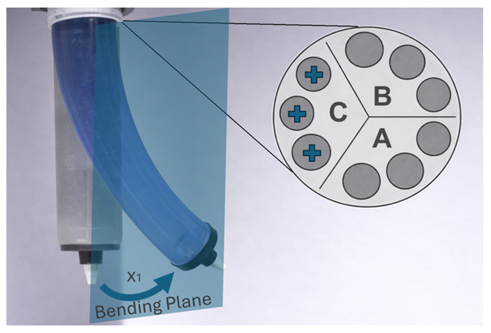
The soft manipulator considered in this work consists of one segment with three sets of internal chambers pressurized independently. When actuated, the manipulator bends on a given plane. The orientation of the bending plane depends on the set of chambers being pressurized, as illustrated in Figure 1.

This work focuses on the dynamics of the manipulator on the bending plane. To this end, the following assumptions are introduced.

Assumption A1.

(Constant curvature and fixed length). The manipulator maintains a constant length and deforms according to a constant curvature (CC) model. The shape of the soft segment can be represented as an arc with unchanging length, with its bending being characterized solely by changes in the radius of the circle that contains this arc. This yields a one-degree-of-freedom (1-DoF) description of its deformed configuration. Because the soft segment is driven by a single bending moment generated through internal pressurization, the model is fully actuated. This assumption is valid as long as the soft segment has a uniform cross section and homogeneous material properties and is not subject to external forces. This approximation provides sufficient accuracy for the system analyzed in this work. The orientation of the tip is indicated by $x_1\in [-\pi ,\pi ]$.

Assumption A2.

The pressure dynamics of the actuation system are neglected (see [19]). This is justified because the pressure states evolve on a much faster timescale than the mechanical dynamics of the manipulator.

The dynamic model of the system, including the hysteretic effects, can be described as follows:

$$\begin{array}{cc}\hfill {\dot{x}}_1& =x_2,\hfill \\ \hfill {\dot{x}}_2& ={\displaystyle \frac{1}{M\left(x_1\right)}}[u-\alpha K\left(x_1\right)x_1-(1-\alpha )K\left(x_1\right)x_3-\left(C(x_1,x_2)+D\right)x_2-G\left(x_1\right)],\hfill \\ \hfill {\dot{x}}_3& =x_2{A}_{\mathrm{hyst}}-\beta |x_2||x_3{|}^{n-1}{x}_3-\gamma x_2{|x_3|}^n,\hfill \\ \hfill y& =\left[\begin{array}{cc}{x}_1& x_2\end{array}\right],\hfill \end{array}$$

(1)

where $x_1$, $x_1$ and $x_3$ correspond to the angular position and angular velocity of the robot tip and to the internal state of the Bouc–Wen model, respectively. The mass $M\left(x_1\right)$, Coriolis effect $C(x_1,x_2)$, stiffness $K(x_1,x_3)$, and gravity $G\left(x_1\right)$ are obtained from a Taylor expansion approximation (i.e., the first four terms) of the dynamics of a constant-curvature segment [8] as follows:

$$\begin{array}{cc}\hfill M\left(x_1\right)& ={\displaystyle \frac{m{L}^2}{3}}{\displaystyle \frac{2x_1-sin\left(2x_1\right)}{2x_1^3}}\hfill \\ \hfill C(x_1,x_2){\dot{x}}_1& =-{\displaystyle \frac{m{L}^2}{3}}{\displaystyle \frac{12x_1-30sin{x}_1+3x_1^{2}sin{x}_1+18x_{1}cos{x}_1+x_1^3}{x_1^6}}{x}_2^2\hfill \\ \hfill G\left(x_1\right)& =-mgL\left(2{\displaystyle \frac{cos\left(x_1\right)-1}{x_1^3}}+{\displaystyle \frac{sin\left(x_1\right)}{x_1^2}}\right)\hfill \end{array}$$

(2)

The resulting expressions for $M\left(x_1\right)$, the Coriolis effect $C(x_1,x_2)$, stiffness $K(x_1,x_3)$, and gravity $G\left(x_1\right)$ are provided in Section 4. The damping coefficient D and stiffness $K\left(x_1\right)$ are obtained experimentally. In particular, there exist positive constants $m_{min}$ and $m_{max}$ such that

$$m_{min}\le M\left(x_1\right)\le m_{max},$$

for all $x_1\in \mathbb{R}$—see [20]. In the same manner,

$$k_{min}\le K\left(x_1\right)\le k_{max},$$

for all $x_1\in \mathbb{R}$. Hysteretic elasticity is described by the Bouc–Wen model, adopting the notation introduced by Song and Der Kiureghian [21]. In particular, $0<\alpha <1,\beta >0,\gamma >0,A_{hyst}>0,andn>0$ are scalar parameters.

Assumption 3.

(Known states and parameters). The position and velocity, $x_1$ and $x_2$, are known, while the hysteresis state $x_3$ is not measured. All model parameters are exactly known. The Bouc–Wen model parameters are defined such that $\beta \ge \gamma >0$ and $n=1$.

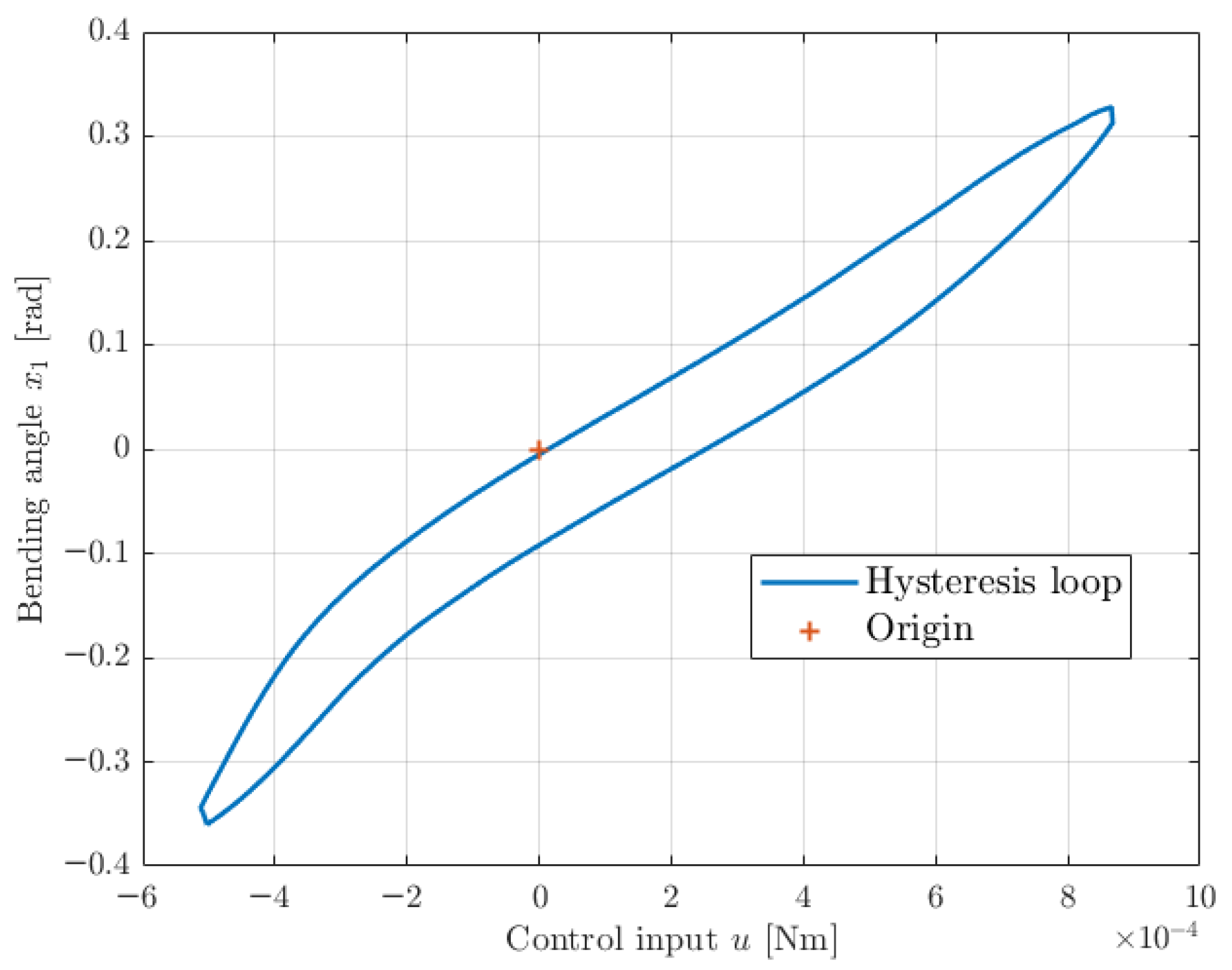
In practice, the parameters are identified experimentally. In particular, $n=1$ is commonly used in both the literature and practical physical applications. For completeness, the case where $n=3$ is discussed in Proposition 3. The condition $\beta >\gamma$ ensures there is a bounded-input, bounded-state (BIBS) of the Bouc–Wen model [22]. A plot showing the hysteresis behavior of our soft manipulator is shown in Figure 2.

A classic Bouc–Wen model fitting for this type of hysteresis loops is studied in detail in [23].

3. Observer-Based State-Feedback Control

The control goal considered in this work is the tracking of the tip rotation of the soft manipulator in an arbitrary bending plane. In order to compensate for the effect of hysteretic elasticity, a state observer and a nonlinear controller are proposed.

3.1. Observer Design

The immersion and invariance methodology [17] is employed to estimate the unknown hysteresis state $x_3$ from measurements of $x_1$ and $x_2$. To this end, the estimation error is defined as follows:

$$e_{x_3}=x_3-{\widehat{x}}_3+\eta ,$$

(3)

where the the state-dependent function $\eta$ and the time derivative of the observer state ${\widehat{x}}_3$ are defined as follows:

$$\begin{array}{cc}\eta \hfill & =L_{obs}M\left(x_1\right)(1-\alpha )x_2,\hfill \\ {\dot{\widehat{x}}}_3\hfill & =L_{obs}(1-\alpha ){\displaystyle \frac{\partial M}{\partial x_1}}{x}_2^2+x_2{A}_{\mathrm{hyst}}-\beta |x_2|({\widehat{x}}_3-\eta )-\gamma x_2|{\widehat{x}}_3-\eta |\hfill \\ \hfill & +L_{obs}(1-\alpha )\left(-\alpha K\left(x_1\right)x_1-(C(x_1,x_2)+D)x_2-(1-\alpha )K\left(x_1\right)({\widehat{x}}_3-\eta )-G\left(x_1\right)+u\right),\hfill \end{array}$$

(4)

with $L_{obs}>0$ serving as a constant tuning parameter.

Proposition 1.

Consider a system (1) corresponding to Assumptions 1, 2, and 3 where the time-derivative of the observer state is given in (4). Consequently, the estimation error e in (3) is bounded and converges to zero exponentially for all $L_{obs}>0$.

Proof. 

Computing the time-derivative of (3) yields

$${\dot{e}}_{x_3}={\dot{x}}_3-{\dot{\widehat{x}}}_3+{\displaystyle \frac{\partial \eta }{\partial x_1}}{x}_2+{\displaystyle \frac{\partial \eta }{\partial x_2}}{\dot{x}}_2.$$

(5)

Substituting (1) and (4) gives

$${\dot{e}}_{x_3}=-L_{obs}{(1-\alpha )}^{2}K\left(x_1\right)e_{x_3}-\beta |x_2|e_{x_3}-\gamma x_2(|x_3|-|{\widehat{x}}_3-\eta |),$$

(6)

Defining the Lyapunov function,

$$V_O={\displaystyle \frac{1}{2}}{e}_{x_3}^2,$$

(7)

and computing its time-derivative while substituting (6) yields

$${\dot{V}}_O=e_{x_3}{\dot{e}}_{x_3}=-L_{obs}{(1-\alpha )}^{2}K\left(x_1\right)e_{x_3}^2-\beta |x_2|e_{x_3}^2-\gamma x_2(|x_3|-|{\widehat{x}}_3-\eta |)e_{x_3},$$

(8)

and, consequently

$${\dot{V}}_O\le -L_{obs}{(1-\alpha )}^{2}K\left(x_1\right)e_{x_3}^2-\beta |x_2|e_{x_3}^2+\gamma |x_2|(||x_3|-|{\widehat{x}}_3-\eta ||)|e_{x_3}|.$$

(9)

Noting that $||x_3|-|{\widehat{x}}_3-\eta ||\le |x_3-{\widehat{x}}_3+\eta |=|e_{x_3}|$, it follows from (9) that

$${\dot{V}}_O\le -L_{obs}{(1-\alpha )}^{2}K\left(x_1\right)e_{x_3}^2-(\beta -\gamma )|x_2|e_{x_3}^2.$$

(10)

Since $\beta >\gamma$ based on Assumption 3, it follows that ${\dot{V}}_O\le -L_{obs}(1-\alpha )k_{\min }{e}_{x_3}^2$—that is ${\dot{V}}_O\le -2L_{obs}(1-\alpha )k_{min}{V}_O$. Thus, $e_{x_3}$ converges to zero exponentially for all $L_{obs}>0$. □

3.2. Controller Design

A control law is designed for tracking the trajectory $q_d\left(t\right)$:

$$\begin{array}{cc}\hfill u& =\alpha K\left(x_1\right)x_1+(C(x_1,x_2)+D)x_2+G\left(x_1\right)+(1-\alpha )K\left(x_1\right)({\widehat{x}}_3-\eta )\hfill \\ \hfill & +\lambda ({\dot{q}}_d-x_2)M\left(x_1\right)+K_{C}M\left(x_1\right)r+{\ddot{q}}_{d}M\left(x_1\right),\hfill \end{array}$$

(11)

with

$$\begin{array}{c}\hfill r=({\dot{q}}_d\left(t\right)-x_2)+\lambda (q_d\left(t\right)-x_1),\end{array}$$

(12)

where $q_d\left(t\right)$ is the desired bending angle, and $K_C$ and $\lambda$ are positive constants.

Proposition 2.

For a system (1) corresponding to Assumptions 1, 2, and 3 in a closed loop with the observer (4) and the control law (11) in place, the estimation error $e_{x_3}$ and tracking error r converge to zero exponentially at a rate of $\sigma >0$ for

$$\begin{array}{cc}\hfill K_C& ={\displaystyle \frac{k_{max}}{2m_{min}}}(1-\alpha )+{\displaystyle \frac{1}{2}}\sigma ,\hfill \\ \hfill L_{obs}& ={\displaystyle \frac{k_{max}}{2m_{min}}}(1-\alpha )+{\displaystyle \frac{1}{2}}\sigma .\hfill \end{array}$$

(13)

Proof. 

The controller Lyapunov function is defined as follows:

$$V_C={\displaystyle \frac{1}{2}}{r}^2.$$

(14)

Computing its time derivative and substituting (1) and (11) yields

$${\dot{V}}_C=-K_C{r}^2-{\displaystyle \frac{r}{M\left(x_1\right)}}K\left(x_1\right)(1-\alpha )(-e_{x_3}),$$

(15)

Defining the new Lyapunov function

$$V_{tot}=V_O+V_C,$$

(16)

and computing its time derivative along the trajectories of the closed-loop system yield

$${\dot{V}}_{tot}\le -\left[\begin{array}{cc}r& e_{x_3}\end{array}\right]\underset{\Omega }{\underbrace{\left[\begin{array}{cc}{K}_C& -{\displaystyle \frac{K\left(x_1\right)}{2M\left(x_1\right)}}(1-\alpha )\\ -{\displaystyle \frac{K\left(x_1\right)}{2M\left(x_1\right)}}(1-\alpha )& L_{obs}{(1-\alpha )}^{2}K\left(x_1\right)\end{array}\right]}}\left[\begin{array}{c}r\\ e_{x_3}\end{array}\right]-(\beta -\gamma )|x_2|e_{x_3}^2.$$

(17)

It follows from Assumption 3 that ${\dot{V}}_{tot}\le -\left[\begin{array}{cc}r& e_{x_3}\end{array}\right]\Omega \left[\begin{array}{c}r\\ e_{x_3}\end{array}\right]<0$, provided that $\Omega \succ 0$, where employing Sylvester’s criterion yields

$$\begin{array}{cc}\hfill K_C& >0,\hfill \\ \hfill L_{obs}{K}_C& >{\displaystyle \frac{K\left(x_1\right)}{4M{\left(x_1\right)}^2}},\hfill \end{array}$$

(18)

with $k_{min}\le K\left(x_1\right)\le k_{max},\forall x_1$ and $M\left(x_1\right)>m_{min},\forall x_1$ as per Assumption 3. Substituting (13) verifies (18) and yields ${\dot{V}}_{tot}\le -{\displaystyle \frac{1}{2}}\sigma (e_{x_3}^2+r^2)$—that is ${\dot{V}}_{tot}\le -\sigma V_{tot}$. Consequently, $e_{x_3}$ and r converge to zero exponentially at a rate of $\sigma$ □

The case $n=3$ is discussed in the following proposition, which requires a stronger condition regarding $\beta$ and $\gamma$, stated as follows.

Assumption 4.

The Bouc–Wen model parameters are defined such that $\beta \ge 3\gamma >0$.

Proposition 3.

Consider the Bouc–Wen hysteretic system in (1) with $n=3$. The observer (4) is modified as follows:

$$\begin{array}{cc}{\dot{\widehat{x}}}_3\hfill & =L_{obs}(1-\alpha ){\displaystyle \frac{\partial M\left(x_1\right)}{\partial x_1}}{x}_2{\dot{x}}_1+x_2{A}_{hyst}-\beta |x_2|{({\widehat{x}}_3-\eta )}^3-\gamma x_2{|{\widehat{x}}_3-\eta |}^3\hfill \\ \hfill & +L_{obs}(1-\alpha )\left(-\alpha K\left(x_1\right)x_1-(C(x_1,x_2)+D)x_2-(1-\alpha )K\left(x_1\right)({\widehat{x}}_3-\eta )-G\left(x_1\right)+u\right).\hfill \end{array}$$

(19)

For a system (1) corresponding to Assumptions 1, 2, 3, and 4 in a closed loop, accounting for the observer (19) and the control law (11), $e_{x_3}$ and r converge to zero exponentially at a rate of $\sigma >0$, provided that (13) is verified.

Proof. 

Computing the time-derivative of (3) and substituting (1) and (19) gives

$${\dot{e}}_{x_3}=-L_{obs}{(1-\alpha )}^{2}K\left(x_1\right)e_{x_3}-\beta |x_2|(x_3^3-{({\widehat{x}}_3-\eta )}^3)-\gamma x_2(|x_3{|}^3-|{\widehat{x}}_3-\eta {|}^3),$$

(20)

where it follows that

$$\begin{array}{cc}\hfill (x_3^3-{({\widehat{x}}_3-\eta )}^3)=& e_{x_3}\underset{{\delta }_{\beta }}{\underbrace{(x_3^2+{({\widehat{x}}_3-\eta )}^2+x_3({\widehat{x}}_3-\eta ))}},\hfill \\ \hfill (|x_3{|}^3-|{\widehat{x}}_3-\eta {|}^3)=& (|x_3|-|{\widehat{x}}_3-\eta |)\underset{{\delta }_{\gamma }}{\underbrace{(|x_3{|}^2+|{\widehat{x}}_3-\eta {|}^2+|x_3||{\widehat{x}}_3-\eta |)}}\hfill \end{array}$$

(21)

Employing Young’s inequality to the cross term of ${\delta }_{\beta }$ and ${\delta }_{\gamma }$ yields

$$\begin{array}{cc}\hfill x_3({\widehat{x}}_3-\eta )\le & {\displaystyle \frac{x_3^2}{2}}+{\displaystyle \frac{{({\widehat{x}}_3-\eta )}^2}{2}},\hfill \\ \hfill |x_3||{\widehat{x}}_3-\eta |\le & {\displaystyle \frac{x_3^2}{2}}+{\displaystyle \frac{{({\widehat{x}}_3-\eta )}^2}{2}},\hfill \end{array}$$

(22)

which, when substituted into ${\delta }_{\beta }$ and ${\delta }_{\gamma }$, yields

$$\begin{array}{cc}\hfill {\displaystyle \frac{1}{2}}\left(x_3^2+{({\widehat{x}}_3-\eta )}^2\right)\le & {\delta }_{\beta }\le {\displaystyle \frac{3}{2}}\left(x_3^2+{({\widehat{x}}_3-\eta )}^2\right),\hfill \\ \hfill {\displaystyle \frac{1}{2}}\left(x_3^2+{({\widehat{x}}_3-\eta )}^2\right)\le & {\delta }_{\gamma }\le {\displaystyle \frac{3}{2}}\left(x_3^2+{({\widehat{x}}_3-\eta )}^2\right).\hfill \end{array}$$

(23)

Computing the time-derivative of (16) and substituting (1) and (11) yield

$$\begin{array}{cc}\hfill {\dot{V}}_{tot}=& -K_C{r}^2-{\displaystyle \frac{r}{M\left(x_1\right)}}K\left(x_1\right)(1-\alpha )(-e_{x_3})-L_{obs}{(1-\alpha )}^{2}K\left(x_1\right)e_{x_3}^2\hfill \\ \hfill & -\beta |x_2|e_{x_3}^2{\delta }_{\beta }-\gamma x_2{e}_{x_3}(|x_3|-|{\widehat{x}}_3-\eta |){\delta }_{\gamma }.\hfill \end{array}$$

(24)

Using $||x_3|-|{\widehat{x}}_3-\eta ||\le |e_{x_3}|$, the following inequality holds:

$$\begin{array}{cc}\hfill \gamma x_2{e}_{x_3}(|x_3|-|{\widehat{x}}_3-\eta |){\delta }_{\gamma }\le & \gamma |x_2||e_{x_3}|||x_3|-|{\widehat{x}}_3-\eta ||{\delta }_{\gamma }\hfill \\ \hfill \le & \gamma |x_2|e_{x_3}^2{\delta }_{\gamma }\hfill \end{array}$$

(25)

Substituting (24) and (25) yields

$$\begin{array}{cc}\hfill {\dot{V}}_{tot}\le & -K_C{r}^2-{\displaystyle \frac{r}{M\left(x_1\right)}}K\left(x_1\right)(1-\alpha )(-e_{x_3})-L_{obs}{(1-\alpha )}^{2}K\left(x_1\right)e_{x_3}^2\hfill \\ \hfill & -\beta |x_2|e_{x_3}^2{\delta }_{\beta }+\gamma |x_2|e_{x_3}^2{\delta }_{\gamma }.\hfill \end{array}$$

(26)

Applying the lower bound on ${\delta }_{\beta }$ and upper bound on ${\delta }_{\gamma }$ from (23) yields

$$\begin{array}{cc}\hfill {\dot{V}}_{tot}\le & -K_C{r}^2+{\displaystyle \frac{K\left(x_1\right)}{M\left(x_1\right)}}(1-\alpha )r{e}_{x_3}-L_{obs}{(1-\alpha )}^{2}K\left(x_1\right)e_{x_3}^2\hfill \\ \hfill & -\left(\beta -3\gamma \right)(x_3^2+{({\widehat{x}}_3-\eta )}^2)|x_2|e_{x_3}^2.\hfill \end{array}$$

(27)

Expressing the quadratic and cross terms in matrix form yields

$$\begin{array}{cc}\hfill {\dot{V}}_{tot}\le & -\left[r{e}_{x_3}\right]\underset{\Omega }{\underbrace{\left[\begin{array}{cc}{K}_C& -{\displaystyle \frac{K\left(x_1\right)}{2M\left(x_1\right)}}(1-\alpha )\\ -{\displaystyle \frac{K\left(x_1\right)}{2M\left(x_1\right)}}(1-\alpha )& L_{obs}{(1-\alpha )}^{2}K\left(x_1\right)\end{array}\right]}}\left[\begin{array}{c}r\\ e_{x_3}\end{array}\right]\hfill \\ \hfill & -\left(\beta -3\gamma \right)(x_3^2+{({\widehat{x}}_3-\eta )}^2)|x_2|e_{x_3}^2\hfill \end{array}$$

(28)

Therefore,${\dot{V}}_{tot}\le -\left[r{e}_{x_3}\right]\Omega \left[\begin{array}{c}r\\ e_{x_3}\end{array}\right]$ due to Assumption 4. Substituting (13) yields, once again, ${\dot{V}}_{tot}\le -{\displaystyle \frac{1}{2}}\sigma (e_{x_3}^2+r^2)$—that is ${\dot{V}}_{tot}\le -\sigma V_{tot}$. Consequently, $e_{x_3}$ and r converge to zero exponentially at a rate of $\sigma$ □

Note that the condition $\beta \ge 3\gamma$ employed in Assumption 4 is in fact conservative, since it follows from Young’s inequalities.

4. Simulation Results

For a soft manipular consisting of one segment with a length $L=56$ mm, a mass $m=6$ g, and a diameter $d=17$ mm, the model parameters were experimentally identified:

$$M\left(x_1\right)=L^{2}m\left({\displaystyle \frac{x_1^4}{\mathrm{25,920}}}-{\displaystyle \frac{x_1^2}{504}}+{\displaystyle \frac{1}{20}}\right),$$

(29)

$$C(x_1,x_2)=-L^{2}m{x}_2\left({\displaystyle \frac{x_1^5}{\mathrm{739,200}}}-{\displaystyle \frac{x_1^3}{\mathrm{12,960}}}+{\displaystyle \frac{x_1}{504}}\right),$$

(30)

$$G\left(x_1\right)=Lgm\left({\displaystyle \frac{x_1^5}{6720}}-{\displaystyle \frac{x_1^3}{180}}+{\displaystyle \frac{x_1}{12}}\right),$$

(31)

$$K\left(x_1\right)=\left(1.2x_1^5+7.3x_1^4+18x_1^3+21x_1^2+21x_1+0.91\right)\times {10}^{-4}.$$

(32)

The damping coefficient is $D=1.91\times {10}^{-5}$, and the Bouc–Wen model parameters are $n=3$, $\alpha =0.62$, $\gamma =0.25$, $A_{\mathrm{hyst}}=0.15$ and $\beta =0.98$. These values were identified experimentally [24].

An adaptive control law [20] was designed to serve as a baseline for comparison with the proposed controller (11):

$$\begin{array}{cc}\hfill u_{\mathrm{adaptive}}& =M\left(x_1\right)a+(C(x_1,x_2)+D)\nu +G\left(x_1\right)+Fr+Y^{\top }\widehat{\theta },\hfill \end{array}$$

(33)

where $Y\left(x_1\right)$ is the ($6\times 1$)-dimensional regressor

$$Y^{\top }=\left[\begin{array}{cccccc}1& x_1& x_1^2& x_1^3& x_1^4& x_1^5\end{array}\right],$$

(34)

$\widehat{\theta }\in {\mathbb{R}}^6$ is the vector of estimated unknown parameters corresponding to the nonlinear stiffness model $K\left(x_1\right)$, and

$$\begin{array}{c}\hfill \nu ={\dot{q}}_d\left(t\right)+\lambda (q_d\left(t\right)-x_1),\\ \hfill a={\ddot{q}}_d\left(t\right)+\lambda ({\dot{q}}_d\left(t\right)-x_2).\end{array}$$

(35)

The update law for the vector $\widehat{\theta }$ is

$$\dot{\widehat{\theta }}=-{\Gamma }^{-1}Yr,$$

(36)

representing a particular case of [5], which refers to the same type of system. Note that the constant coefficient in $K\left(x_1\right)$ accounts for a constant additive disturbance, which is representative of the effect of Bouc–Wen hysteresis in a steady state. The tuning parameters for this controller are the gain $F>0$, the gain $\lambda >0$, and the matrix $\Gamma \succ 0$.

The trajectory-tracking performance of the proposed controller was simulated in MATLAB using an ODE23 solver. The tuning parameters for both controllers are $K_C=80$, $\lambda =12$$L_{Obs}=3000$, $F=0.00015$, $\lambda =7$, and $\Gamma =200{\mathbb{I}}_{6\times 6}$. In particular, $F,\lambda ,and\Gamma$ were chosen to obtain a step response similar to that of the proposed controller (11).

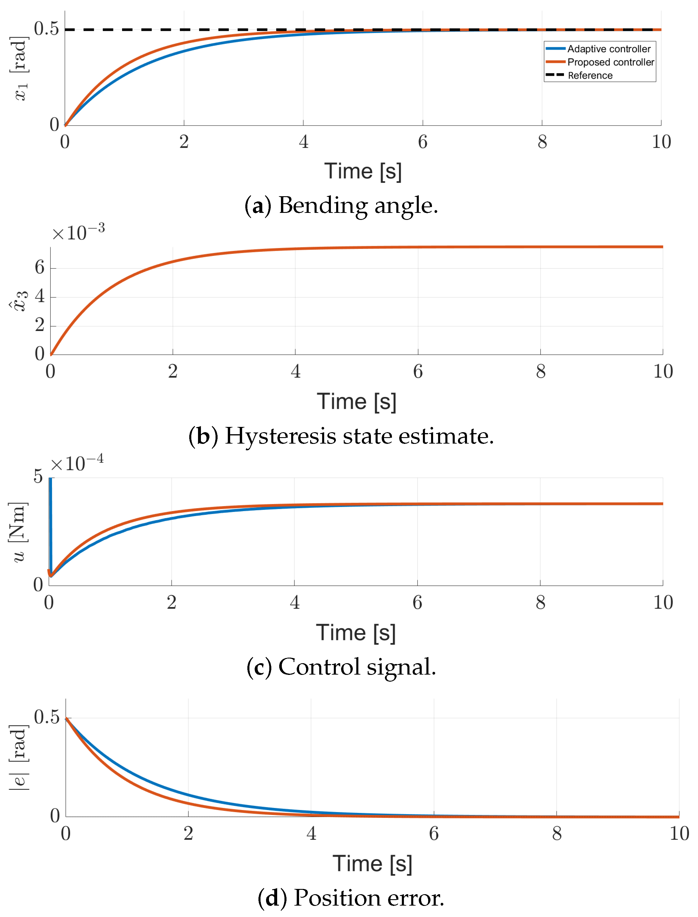
The step response is shown in Figure 3. Both controllers (11) and (33) achieve a steady-state error pf zero with comparable settling times, as a result of the chosen tuning strategy. This is expected, since the net contribution of hysteretic elasticity in a steady state is a constant disturbance, which is accounted for by the constant term in the regressor Y.

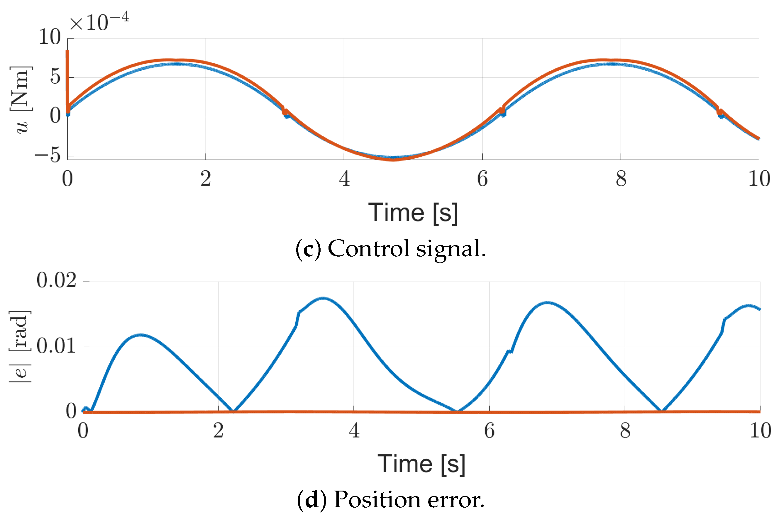
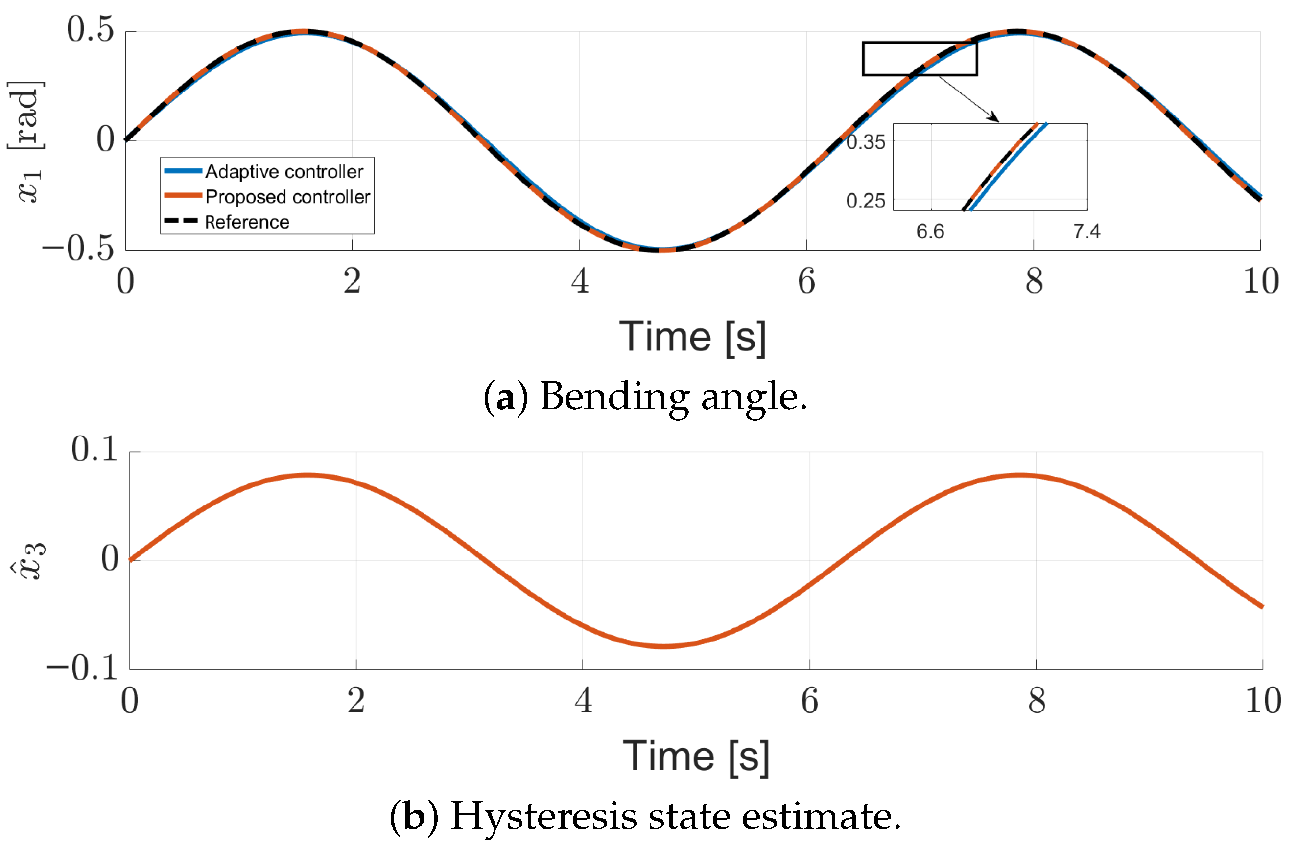
In order to test the system’s tracking response and highlight the difference between the new controller (11) and the baseline (33), a sinusoidal reference signal was defined:

$$[q_d,{\dot{q}}_d,{\ddot{q}}_d]=[0.5sin\left(t\right),0.5cos\left(t\right),-0.5sin\left(t\right)].$$

(37)

The response is shown in Figure 4. Note that the proposed controller (11) yields a smaller tracking error compared to the baseline (33). Note that the same tuning used in the step response has been used here. This confirms that hysteretic elasticity cannot be accurately represented as an adaptive nonlinear stiffness (i.e., with the regressor Y).

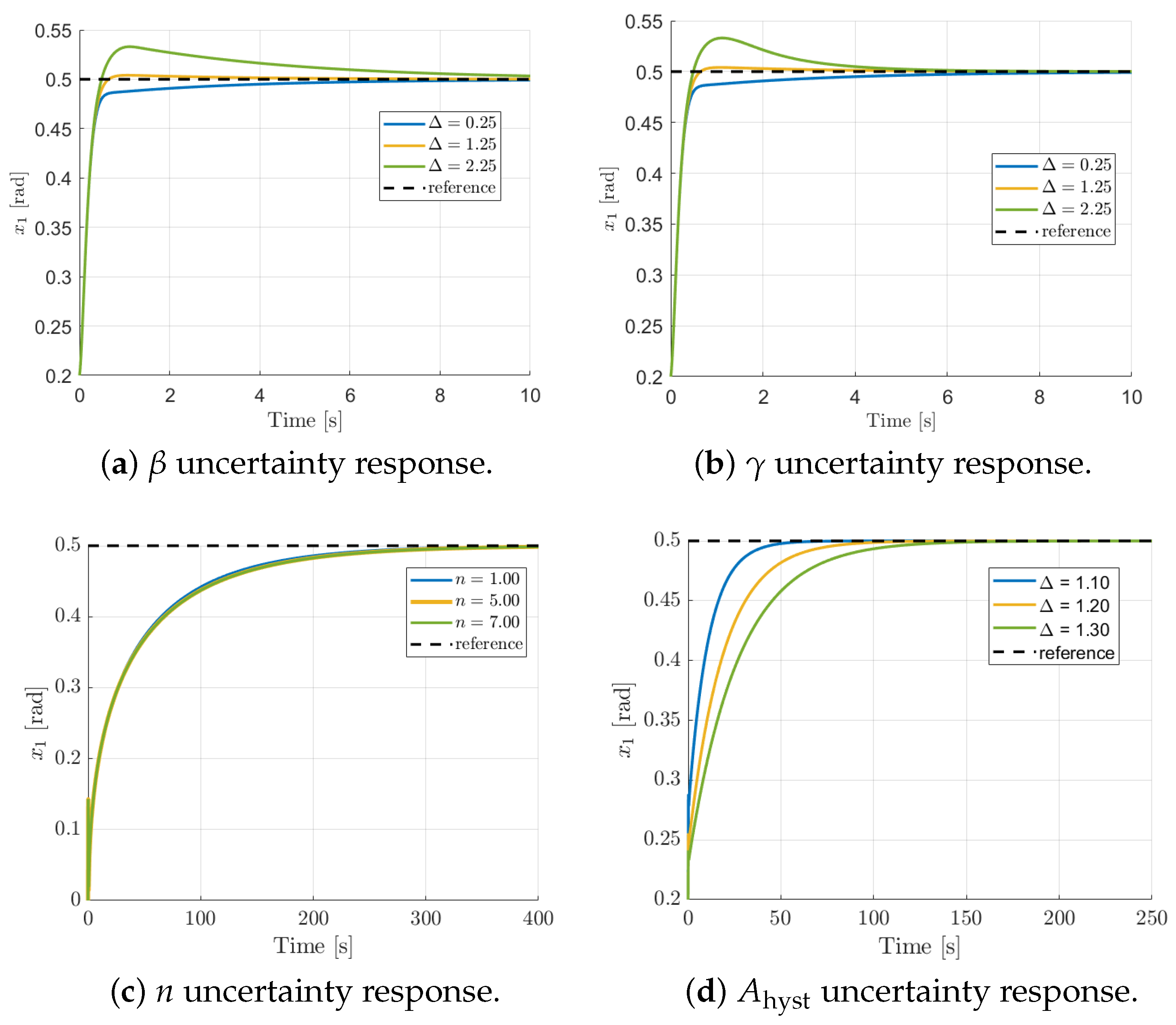
In order to account for parameter mismatch and uncertainties, relative variations in each hysteresis parameter($A_{hyst}$, $\gamma$ and $\beta$) are considered, wherein each parameter is multiplied by a coefficient ($\Delta$) in the model, but the nominal value is employed in the controller (11). For the parameter n, the controller and observer use $n=3$, while the model is tested for different values of n.

Figure 5 shows that even with significant mismatches in the Bouc–Wen model parameters, the proposed controller yields a steady-state error of zero.

5. Experimental Results

5.1. Experimental Setup

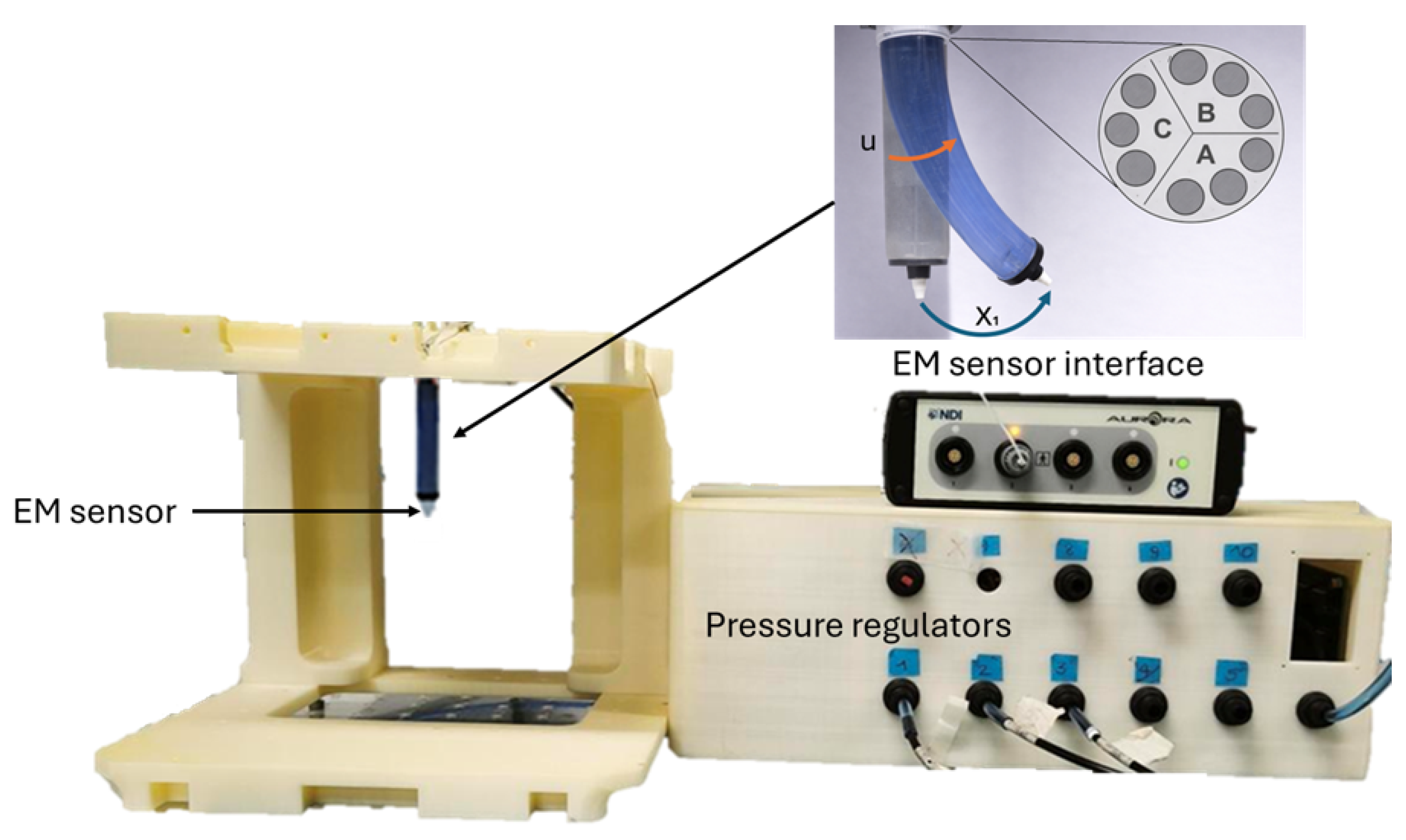
Experiments were performed on a soft continuum manipulator described in [25,26]. The experimental setup, shown in Figure 6, consists of three proportional pneumatic regulators (i.e., TeCNO Basic, Hoergiber, Germany) that regulate three pressure channels for the manipulator (i.e., $P_A$, $P_B$, and $P_C$), yielding a pressure range of 0 to 2.5 Bar on each channel. The valves are controlled with a micro-controller (NXP LPC1768, Mbed) via an SPI bus. The tip orientation of the manipulator is measured with an accuracy of 0.035 radians using an electromagnetic (EM) sensor (Aurora, NDI). All components communicate with MATLAB R2023b via serial links.

For the experimental results, the controller and observer gains for (11) were set to $K_C=80$, $\lambda =12$ and $L_{Obs}=3000$, as in the simulation results. For the baseline controller (33), the tuning parameters F and $\lambda$ were the same as in the simulations, while the matrix $\Gamma$ was set to $\Gamma =diag(\mathrm{10,000},1000,100,10,10,10)$. This different tuning was required in order to preserve responsiveness owing to the larger uncertainties in the experimental setup relative to the simulations.

5.2. Step Response

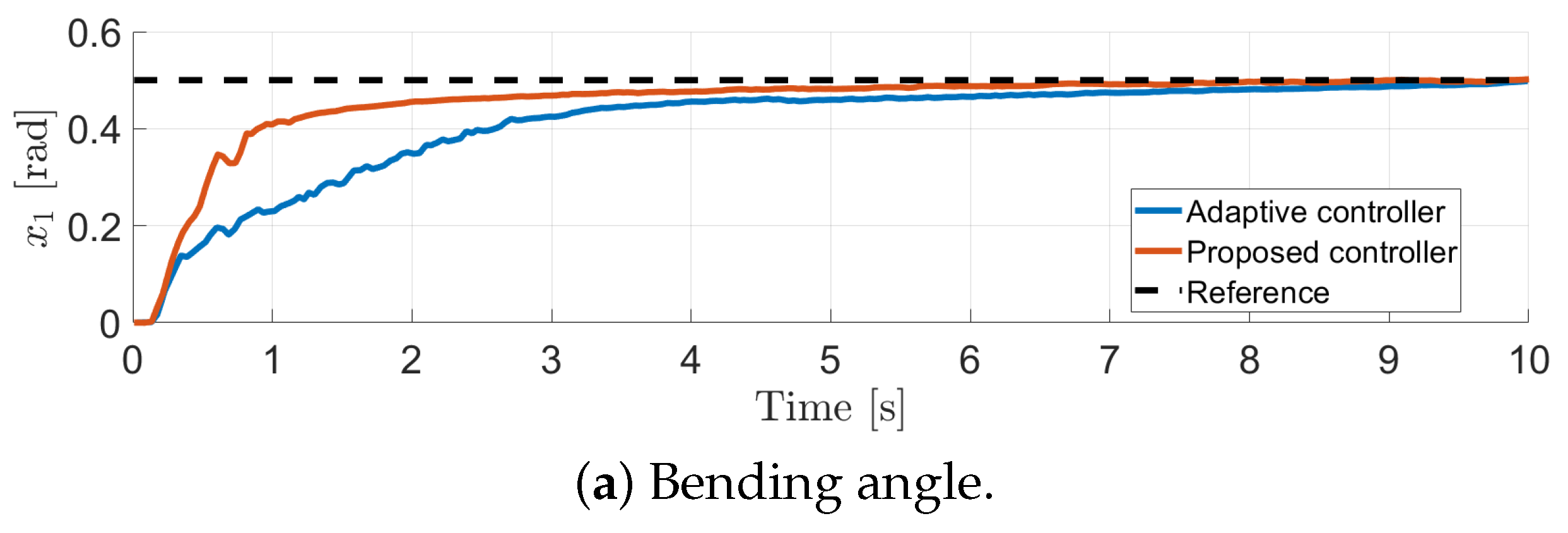
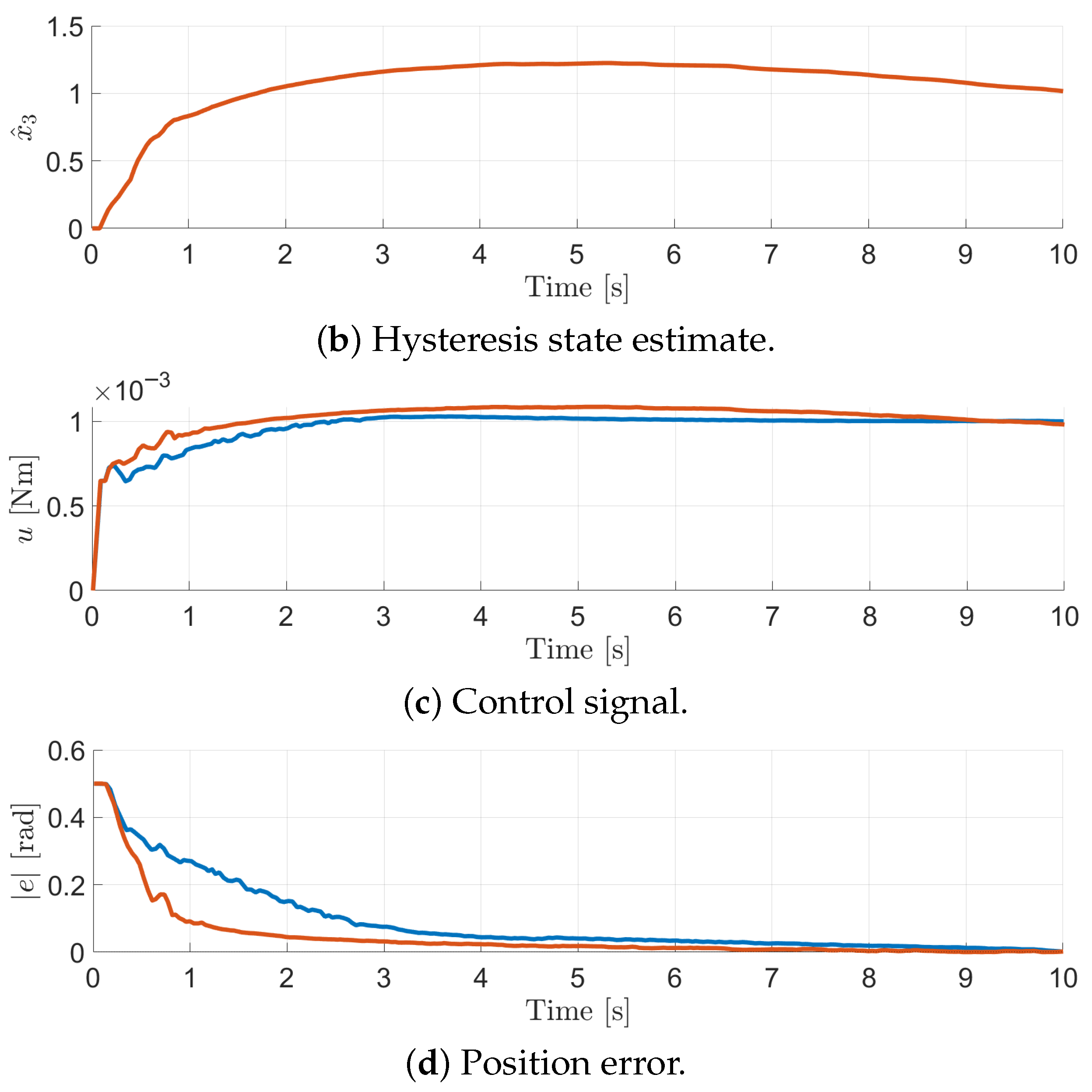
Figure 7 shows that both the proposed controller (11) and the baseline (33) yield a steady-state error of zero. With the tuning employed, the proposed controller (11) shows a slightly faster response, which is in agreement with the simulation results.

5.3. Sinusoidal Response

In order to compare the tracking performances of both controllers, a sinusoidal reference trajectory was set, as in (37).

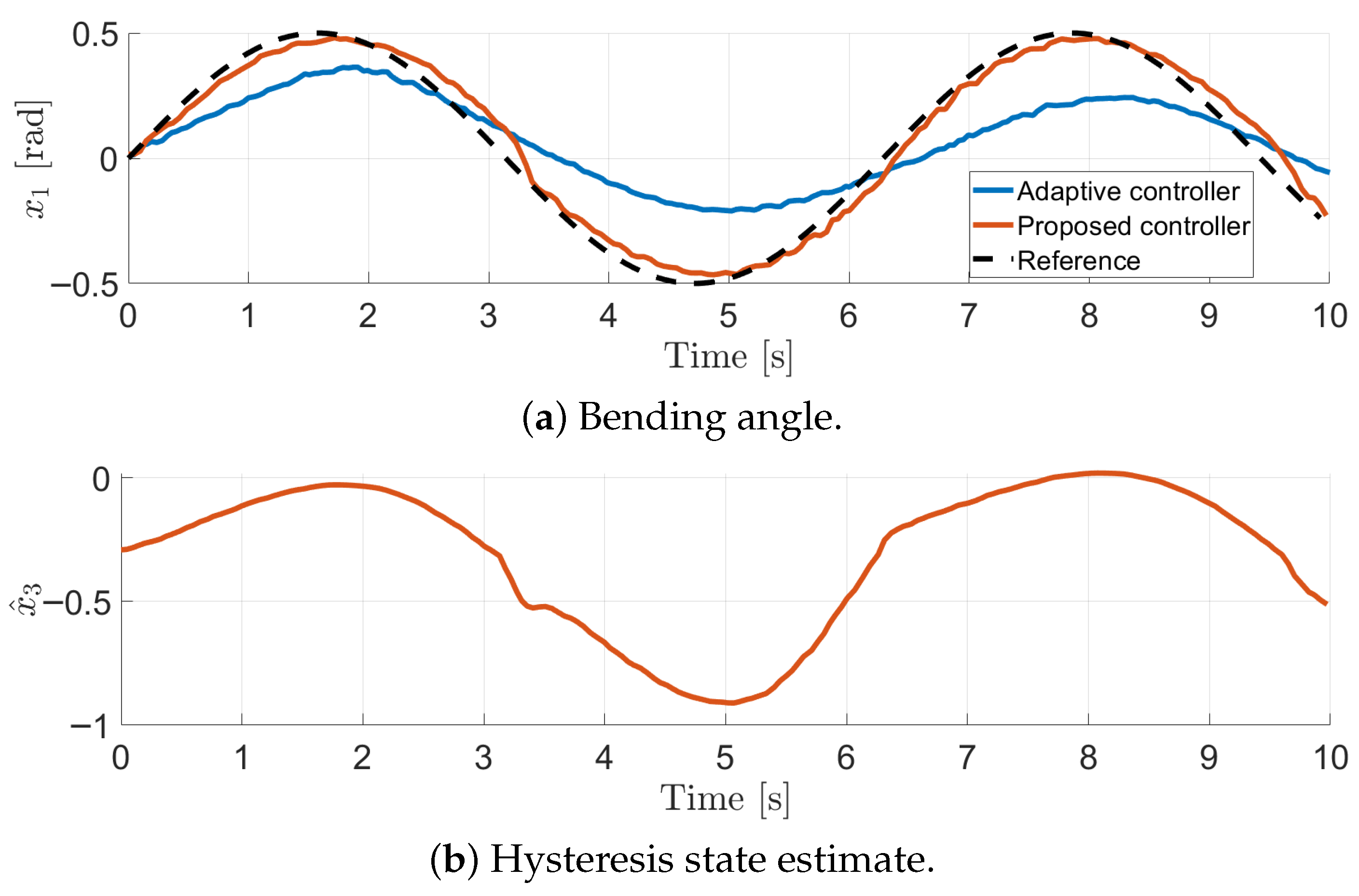
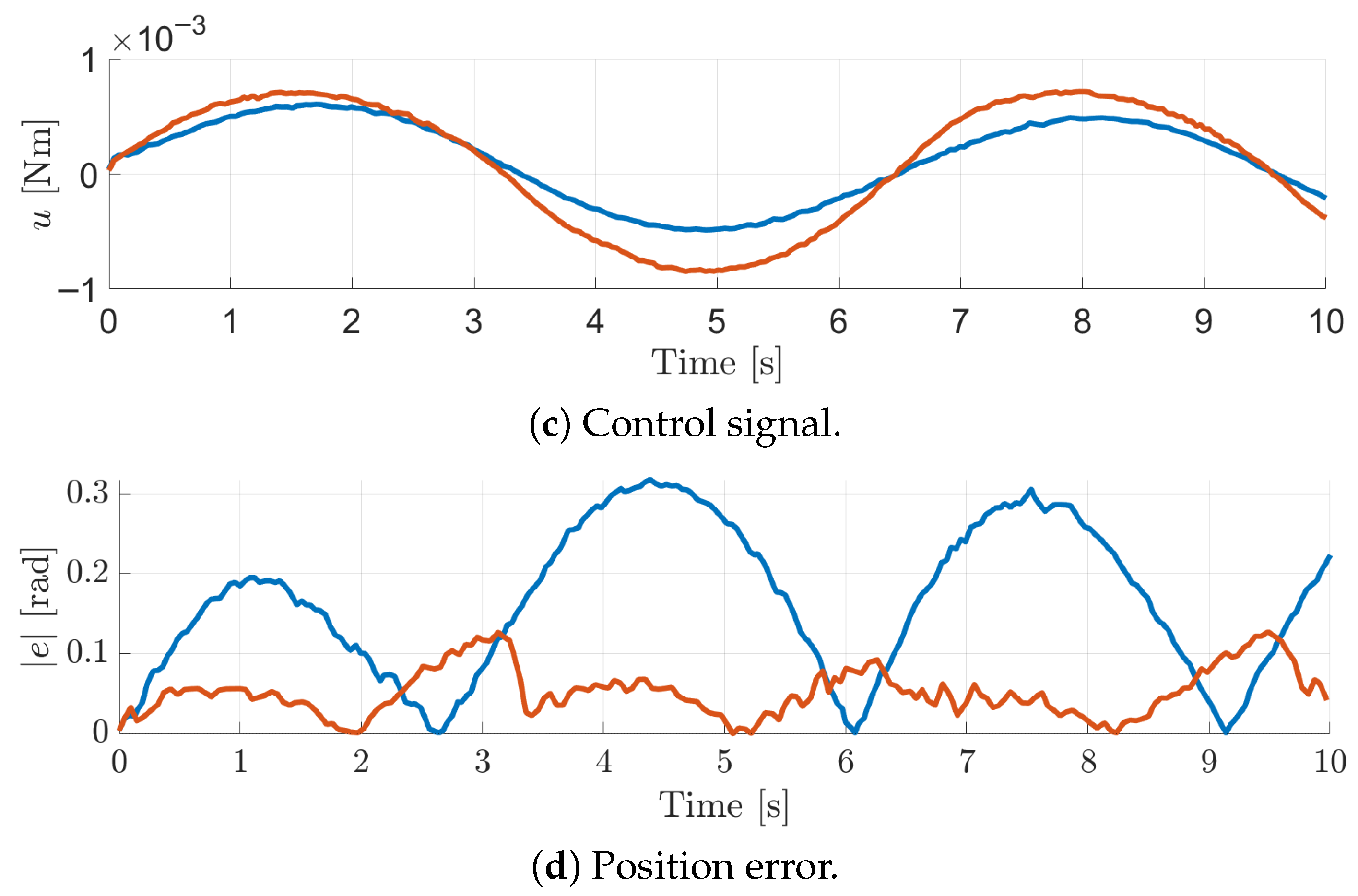
Figure 8 shows that the proposed controller (11) yields a smaller tracking error compared to the baseline (33), which is in agreement with the simulations.

Table 1. Root Mean Square Error (RMSE) of the controllers in simulation and experimental tests.

RMSE [rad]
Controller	Simulation		Experiments
	Step	Sine	Step	Sine
Adaptive control (33)	0.1226	0.0098	0.1358	0.2030
Proposed controller (11)	0.1170	0.0002	0.0769	0.1020

presents the corresponding RMSE values for each controller under step and sinusoidal reference inputs, for both simulation and experimental results.

In summary, both the simulations and experiments indicate that the proposed controller (11) performs best in the tracking task. This suggests that the Bouc–Wen model provides an accurate representation of elastic hysteresis in the soft manipulator and that the proposed controller can effectively compensate for its effects on system dynamics.

5.4. Robustness to Disturbances

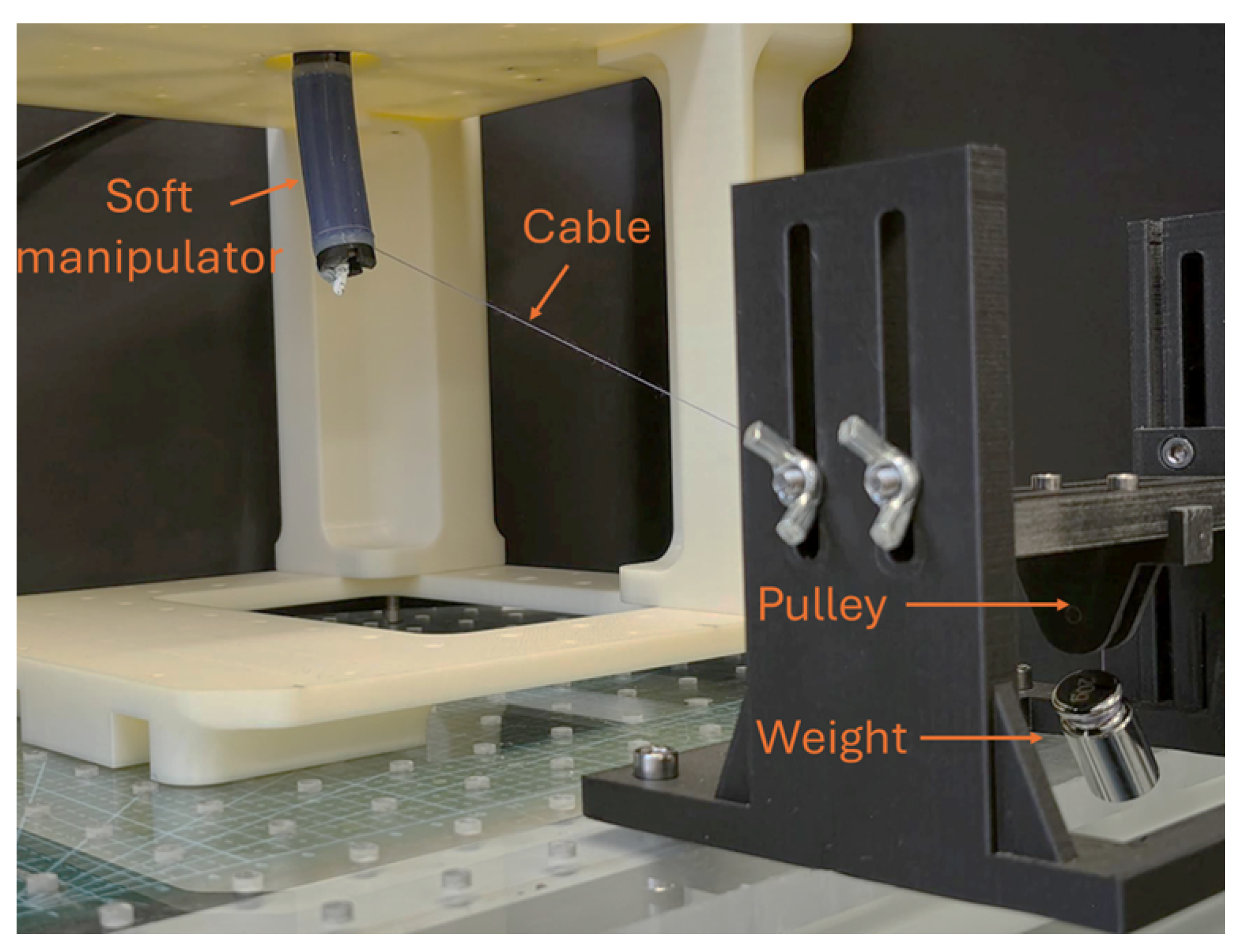
To evaluate the robustness and performance limits of the proposed controller, various weights were attached to the manipulator tip through a pulley mechanism to induce in-plane disturbances. The experimental setup is shown in Figure 9. Note that this experimental scenario does not conform with Assumption 1 since CC generally does not hold in the presence of external forces. Nevertheless, the magnitude of the external force is such that, in practice, the CC model remains representative of the real system. To this end, note that the tip position error with the external load resulting from the CC approximation, computed relative to the tip displacement of the no-load case, is approximately 0.78% at 5 g, 1.53% at 10 g, and 3.14% at 20 g.

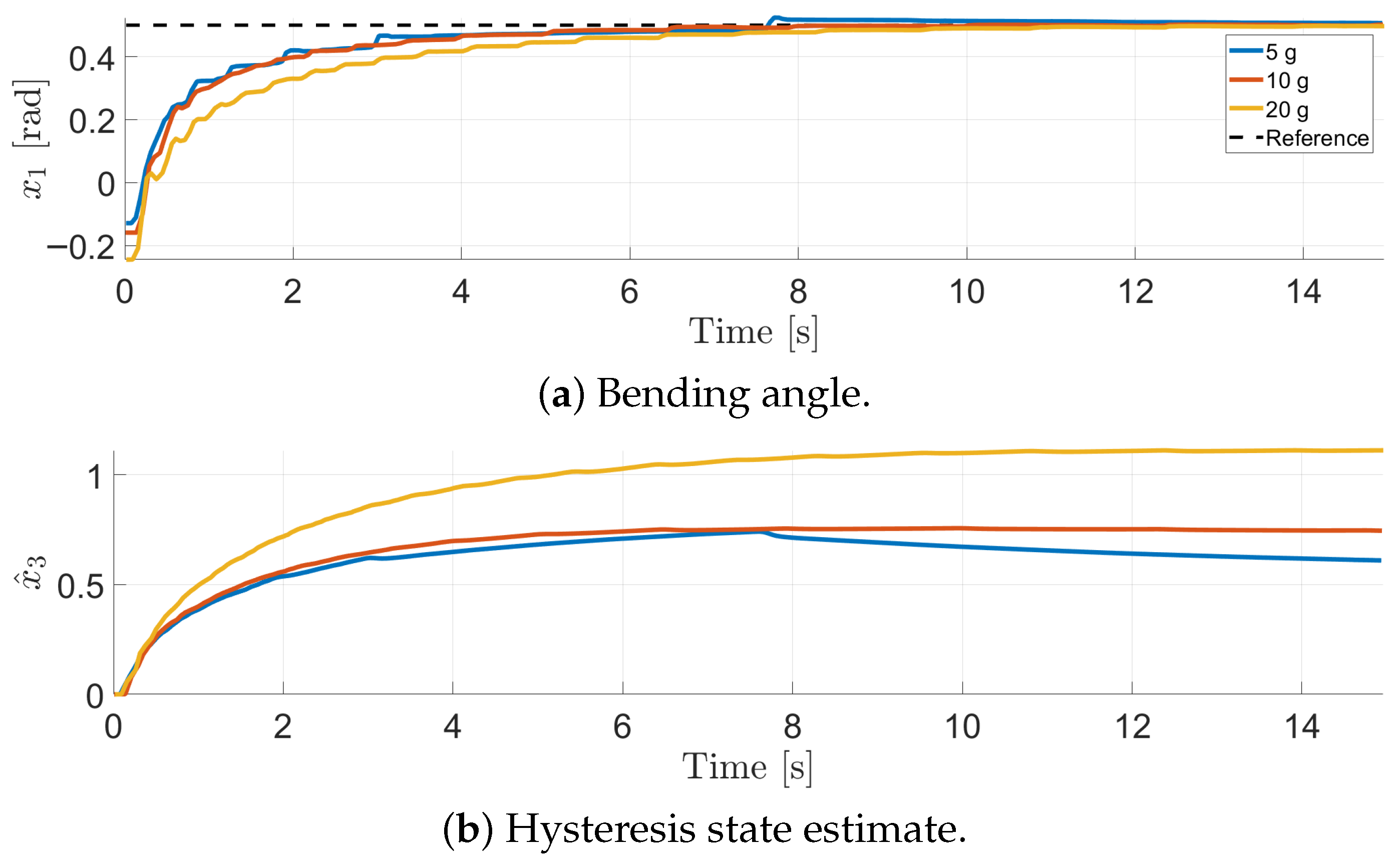
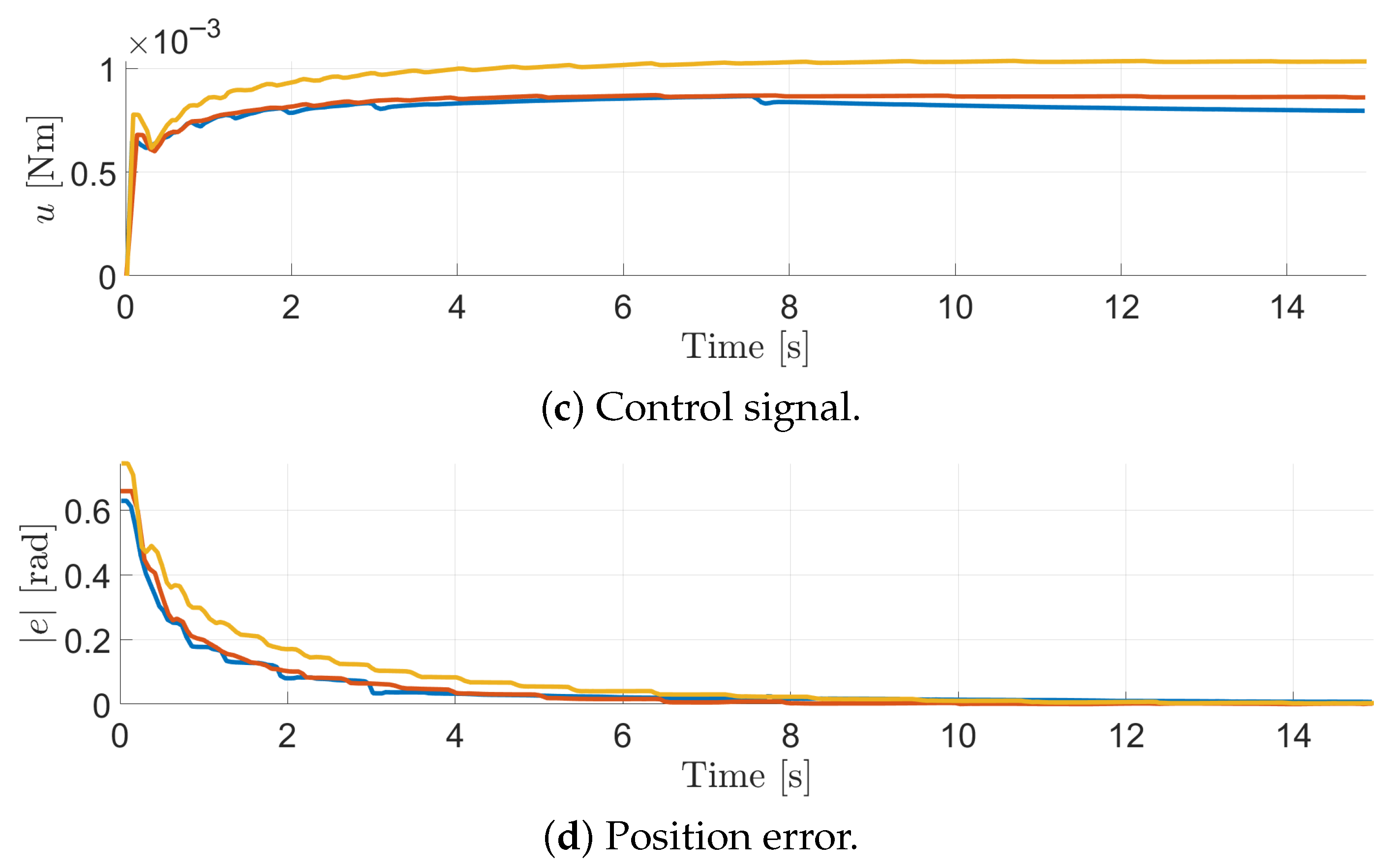
Regulation to a setpoint was successfully achieved with the proposed controller for different weights attached to the manipulator, ranging from 5 to 20 g.

The Integral of Absolute Error (IAE) was used to assess controller performance, allowing direct comparison with [5]. Under no-load conditions, the proposed controller (11) achieved an IAE of 0.49 rad, representing a 50% reduction compared to the adaptive controller (33) (IAE = 1.00 rad) and performing comparably to SMC (IAE = 0.312 rad), Lyapunov redesign (IAE = 0.473 rad), and the adaptive controller proposed in [5] (IAE = 0.753 rad), which refer to a similar prototype. In the presence of external loads, the proposed controller (11) yielded a stable response, whereas the adaptive controller (33) resulted in large oscillations. No tests with external loads were reported in [5].

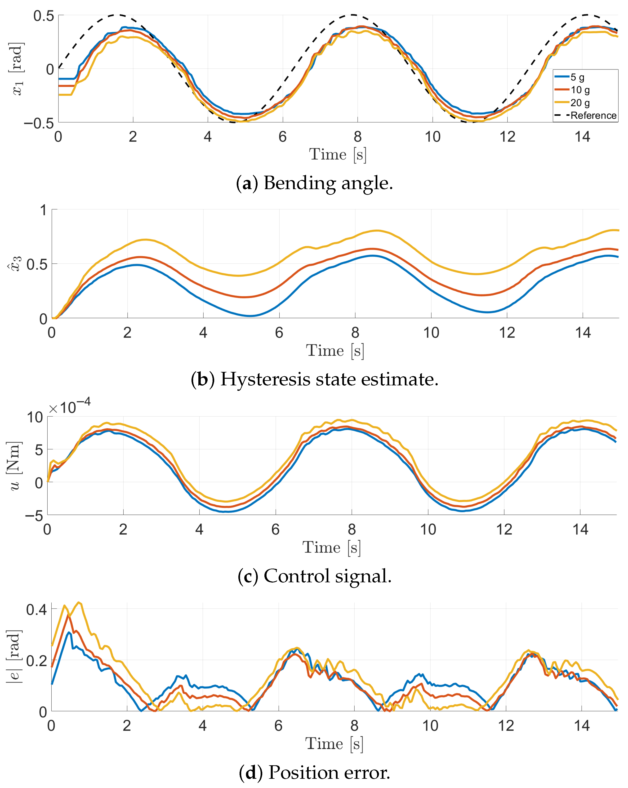
Figure 10 and Figure 11 shows that the proposed controller has satisfactory performance in regulating a step reference and tracking a sinusoidal reference reference (37) with weights up to 20 g.

The difference between 5 g and 20 g is relatively small, whereas the change from no load to 5 g is more noticeable. This may be due to friction between the cable and pulley, which adds to the load and is not present in the no-load condition.

In summary, the results suggest that the proposed controller (11) is robust to additional disturbances that result from interactions with the environment. This is particularly desirable for surgical applications, where the manipulator can interact with tissues during tasks such as suturing and resection.

6. Conclusions

An observer was designed to account for hysteretic elasticity in a soft continuum manipulator. Combining the observer with a model-based controller enhanced tracking performance and robustness to disturbances. Comparison with a traditional adaptive controller indicated that the proposed controller is better suited to compensating for the effects of hysteretic elasticity.

Future work will investigate the inclusion of pressure dynamics in the model in an attempt to further improve tracking accuracy. In addition, given the digital application of the controller, future work should explore a control design in discrete time. Finally, extending the present work to three-dimensional motion remains an important direction for future research.

References

1. Runciman, M.S.; Darzi, A.; Mylonas, G.P. Soft Robotics in Minimally Invasive Surgery. Soft Robot. 2019, 6, 423–443. [Google Scholar] [CrossRef]
2. Trivedi, D.; Rahn, C.D.; Kier, W.M.; Walker, I.D. Soft Robotics: Biological Inspiration, State of the Art, and Future Research. Appl. Bionics Biomech. 2008, 5, 99–117. [Google Scholar] [CrossRef]
3. Alici, G. Softer is Harder: What Differentiates Soft Robotics from Hard Robotics? MRS Adv. 2018, 3, 1557–1568. [Google Scholar] [CrossRef]
4. Preisach, F. Über Die Magnetische Nachwirkung. Z. Phys. 1935, 94, 277–302. [Google Scholar] [CrossRef]
5. Wang, L.; Chen, K.; Franco, E. Robust and Adaptive Control of a Soft Continuum Manipulator for Minimally Invasive Surgery. Robotics 2024, 13, 162. [Google Scholar] [CrossRef]
6. Della Santina, C.; Bianchi, M.; Grioli, G.; Angelini, F.; Catalano, M.G.; Garabini, M.; Bicchi, A. Controlling Soft Robots: Balancing Feedback and Feedforward Elements. IEEE Robot. Autom. Mag. 2017, 24, 75–83. [Google Scholar] [CrossRef]
7. Heredia-Pérez, M.; Alvarez, D.A.; Bedoya-Ruiz, D. A State-of-the-Art Review of the Bouc-Wen Class Model of Hysteresis: Origin, Evolution and Current State. Arch. Comput. Methods Eng. 2025, 33, 1–51. [Google Scholar] [CrossRef]
8. Della Santina, C.; Duriez, C.; Rus, D. Model-Based Control of Soft Robots: A Survey of the State of the Art and Open Challenges. IEEE Control Syst. Mag. 2023, 43, 30–65. [Google Scholar] [CrossRef]
9. Franco, E.; Ayatullah, T.; Sugiharto, A.; Garriga-Casanovas, A.; Virdyawan, V. Nonlinear energy-based control of soft continuum pneumatic manipulators. Nonlinear Dyn. 2021, 106, 229–253. [Google Scholar] [CrossRef]
10. Donaire, A.; Romero, J.G.; Ortega, R.; Siciliano, B. Robust IDA-PBC for Underactuated Mechanical Systems Subject to Matched Disturbances. Int. J. Robust Nonlinear Control 2017, 27, 1000–1016. [Google Scholar] [CrossRef]
11. Ortega, R.; Spong, M.W.; Gomez-Estern, F.; Blankenstein, G. Stabilization of a Class of Underactuated Mechanical Systems via Interconnection and Damping Assignment. IEEE Trans. Autom. Control 2002, 47, 1218–1233. [Google Scholar] [CrossRef]
12. Franco, E.; Garriga Casanovas, A.; Donaire, A. Energy shaping control with integral action for soft continuum manipulators. Mech. Mach. Theory 2021, 158, 104250. [Google Scholar] [CrossRef]
13. Yi, B.; Fan, Y.; Liu, D.; Guadalupe Romero, J. Simultaneous Position-and-Stiffness Control of Underactuated Antagonistic Tendon-Driven Continuum Robots. IEEE Trans. Autom. Sci. Eng. 2025, 22, 7238–7254. [Google Scholar] [CrossRef]
14. Grube, M.; Wieck, J.C.; Seifried, R. Comparison of Modern Control Methods for Soft Robots. Sensors 2022, 22, 9464. [Google Scholar] [CrossRef]
15. Asgari, M.; Magerand, L.; Manfredi, L. A review on model-based and model-free approaches to control soft actuators and their potentials in colonoscopy. Front. Robot. AI 2023, 10, 1236706. [Google Scholar] [CrossRef]
16. Astolfi, A.; Ortega, R. Immersion and Invariance: A New Tool for Stabilization and Adaptive Control. IEEE Trans. Autom. Control 2003, 48, 590–606. [Google Scholar] [CrossRef]
17. Astolfi, A.; Karagiannis, D.; Ortega, R. Nonlinear and Adaptive Control with Applications; Number 1 in Communications and Control Engineering Series; Springer: London, UK, 2007; p. 290. [Google Scholar] [CrossRef]
18. Franco, E.; Garriga-Casanovas, A.; Tang, J.; Rodriguez y Baena, F.; Astolfi, A. Adaptive Energy Shaping Control of a Class of Nonlinear Soft Continuum Manipulators. IEEE/ASME Trans. Mechatron. 2022, 27, 280–291. [Google Scholar] [CrossRef]
19. Franco, E.; Garriga-Casanovas, A. Energy Shaping Control of Soft Continuum Manipulators with in-plane Disturbances. Int. J. Robot. Res. 2021, 40, 236–255. [Google Scholar] [CrossRef]
20. Spong, M.; Hutchinson, S.; Vidyasagar, M. Robot Modeling and Control; Wiley: Hoboken, NJ, USA, 2006; Volume 33, p. 403. [Google Scholar] [CrossRef]
21. Song, J.; Der Kiureghian, A. Generalized Bouc–Wen Model for Highly Asymmetric Hysteresis. J. Eng. Mech. 2006, 132, 610–618. [Google Scholar] [CrossRef]
22. Ikhouane, F.; Rodellar, J. Systems with Hysteresis: Analysis, Identification and Control Using the Bouc-Wen Model; John Wiley & Sons: Hoboken, NJ, USA, 2007; p. 202. [Google Scholar] [CrossRef]
23. De la Morena, J.; Ramos, F.; Vázquez, A.S. Hysteresis Modeling of Soft Pneumatic Actuators: An Experimental Review. Actuators 2025, 14, 321. [Google Scholar] [CrossRef]
24. Bassett, B.D.; Dias, A.; Shi, J.; Shakib, F.; Franco, E.; Chen, K. Multi-Modal LSTM-Based Tracking Control for a Soft Robotic Manipulator with Hysteresis. In Proceedings of the 25th European Control Conference (ECC), Reykjavik, Iceland, 7–10 July 2026. in press. [Google Scholar]
25. Franco, E.; Aktas, A.; Treratanakulchai, S.; Garriga-Casanovas, A.; Donder, A.; Rodriguez y Baena, F. Discrete-time model based control of soft manipulator with FBG sensing. In Proceedings of the 2023 IEEE International Conference on Robotics and Automation (ICRA), London, UK, 29 May–2 June 2023; pp. 567–572. [Google Scholar] [CrossRef]
26. Shi, J.; Jin, H.; Abad, S.A.; Gaozhang, W.; Shi, G.; Wurdemann, H.A. A static modeling and evaluation framework for soft continuum robots with reinforced chambers. IEEE Trans. Robot. 2025, 41, 6419–6439. [Google Scholar] [CrossRef]
Figure 1. Soft manipulator prototype. Detailed view of internal chambers and corresponding bending plane.
Applsci 16 03807 g001
Figure 2. Soft manipulator hysteretic loop.
Applsci 16 03807 g002
Figure 3. Comparison of simulation step responses between the proposed controller (11) and the baseline (33).
Applsci 16 03807 g003
Figure 4. Comparison of simulation sine responses between the proposed controller (11) and baseline (33).
Applsci 16 03807 g004aApplsci 16 03807 g004b
Figure 5. System response with controller (11) and uncertain model parameters.
Applsci 16 03807 g005
Figure 6. Experimental setup consisting of pressure regulators, an NDI Aurora electromagnetic tracking system, and a pneumatically actuated soft manipulator.
Applsci 16 03807 g006
Figure 7. Comparison of experimental step responses between proposed controller (11) and baseline (33), with K C = 80 , λ = 12 , L O b s = 3000 .
Applsci 16 03807 g007aApplsci 16 03807 g007b
Figure 8. Comparison of experimental sine responses between proposed controller (11) and baseline (33).
Applsci 16 03807 g008aApplsci 16 03807 g008b
Figure 9. Experimental setup, with weights attached to the manipulator tip to generate in-plane disturbances.
Applsci 16 03807 g009
Figure 10. Experimental step response with different weights for the proposed controller (11).
Applsci 16 03807 g010aApplsci 16 03807 g010b
Figure 11. Comparison of experimental sine responses with different weights.
Applsci 16 03807 g011