Article

Machine Learning-Assisted Modal Sensitivity and Parameter Ranking in Systems with Viscoelastic Damping


by
Jakub Porysek
1 and
Magdalena Łasecka-Plura
2,*
1
Independent Researcher, 61-131 Poznan, Poland
2
Institute of Structural Analysis, Poznan University of Technology, ul. Jacka Rychlewskiego 1, 61-131 Poznan, Poland
*
Author to whom correspondence should be addressed.
Appl. Sci. 2026, 16(8), 3749; https://doi.org/10.3390/app16083749
Submission received: 9 March 2026 / Revised: 3 April 2026 / Accepted: 7 April 2026 / Published: 11 April 2026
(This article belongs to the Section Civil Engineering)

Abstract

This paper proposes a machine-learning-assisted framework for modal sensitivity analysis of systems with viscoelastic damping elements, including both classical and fractional rheological models. Surrogate models are trained to approximate natural frequencies over a prescribed parameter space using two sampling strategies (Grid and Latin Hypercube) and two regression approaches: multi-layer perceptron (MLP) and Gaussian process regression (GPR). Sensitivities are obtained from the surrogates by finite differences and complemented by model-interpretability measures, namely permutation feature importance (PFI) and Shapley Additive Explanations (SHAP). The surrogate-based results are compared with analytically obtained sensitivities. Local first- and second-order sensitivities of natural frequencies are derived analytically using the direct differentiation method (DDM) for a nonlinear eigenvalue problem formulated in the Laplace domain and further transformed into dimensionless sensitivity measures. The methodology is demonstrated for a single-degree-of-freedom oscillator with classical and fractional Kelvin damper models and a two-story frame equipped with a fractional Kelvin damper. The results show very good agreement between analytical and surrogate-based sensitivities. Feature-importance rankings obtained by PFI and SHAP are consistent with the dimensionless sensitivities and capture changes in parameter influence under varying damping levels. Dispersion studies indicate only minor ranking variations.

1. Introduction

Viscoelastic elements are currently among the most frequently used solutions for passive vibration reduction in engineering structures. They cover a wide range of applications, including damping layers and cores of sandwich beams and plates [1,2], vibration dampers described by classical and fractional rheological models [3], as well as joints and connections with viscoelastic properties [4]. A broad review of the dynamics of systems with viscoelastic elements can be found in [5]. These solutions make it possible to effectively reduce vibration amplitudes, improving user comfort and structural durability. At the same time, viscoelasticity is characterized by a frequency dependence of material properties, which means that the structural response may change significantly even for small perturbations of design parameters. Therefore, sensitivity analysis [6,7] is an important tool in the design of structures with viscoelastic elements, enabling the identification of dominant parameters, supporting optimization procedures [8], and assessing the effect of uncertainty in input parameters on the dynamic response of the system [9].
Classical local sensitivity analysis in structural dynamics is based on computing derivatives of response quantities with respect to design parameters, in particular derivatives of eigenvalues and eigenvectors, as well as characteristics in the frequency domain such as the frequency response function (FRF). The main approaches include the modal method [10], Nelson’s method [11], later extended to systems with viscous and non-viscous damping [12,13], and algebraic methods. The latter includes the direct differentiation method (DDM), applied to systems with distinct and repeated eigenvalues [14] and to systems with viscous and non-viscous damping [15,16], as well as the adjoint variable method (AVM), described for systems with distinct and repeated eigenvalues in [17,18]. Detailed formulations of DDM and AVM for systems with viscoelastic elements, including both first- and second-order sensitivities, are presented in [19,20], while [21] further extends DDM to systems with repeated eigenvalues.
Analytical sensitivity analysis, although accurate, can be computationally expensive in dynamic problems. The DDM approach requires repeated solutions of the governing equations for successive parameters, whereas the AVM approach involves solving additional adjoint problems. This becomes particularly evident in studies accounting for uncertainty in design parameters [22]. In stochastic approaches, the computational cost further increases, especially when second-order accuracy is sought [23], and similar difficulties arise in random vibration problems of coupled systems [24]. Accordingly, it is natural to seek approaches that provide sensitivity information with a smaller number of computationally expensive simulations.
One direction is to construct a surrogate model using machine learning, which approximates the relationship between input parameters and the system response and enables sensitivity analyses to be carried out with a reduced number of full simulations. In general, data-driven predictive models can be used to approximate complex material relationships trained on micromechanical simulations [25], to rapidly evaluate responses in failure mechanics problems [26], or to predict the load-carrying capacity of structural components using soft-computing techniques [27]. In the field of dynamics, artificial neural networks (ANNs), deep neural networks (DNNs), and probabilistic models such as Kriging or Gaussian process regression (GPR), trained on finite element method (FEM) results, have been widely used to predict natural frequencies for new parameter configurations. Examples include sandwich plates with a viscoelastic core [28], laminated composite plates [29], and frequency prediction based directly on measurement data [30]. Regression-based neural networks have also been applied to vibrating plates [31] and annular plates [32], while Kriging and polynomial neural networks have been used in stochastic free-vibration analysis of composite structures with uncertain parameters [33,34]. An alternative to neural-network-based surrogate models is the PC-NARX approach proposed in [35] for dynamic problems with parameter uncertainty.
Machine learning models can be used not only for response prediction but also for efficient sensitivity analysis, either by performing sensitivity analysis directly on a surrogate model or by applying tools that quantify the contribution of input variables. In the first case, the computational cost of estimating sensitivity measures is reduced by analyzing the metamodel instead of performing expensive finite element simulations. Examples include a hybrid polynomial-chaos–Kriging metamodel for global sensitivity analysis in a rotordynamics problem with uncertainties [36], a Gaussian Process model used for both local and global sensitivity analyses in nonlinear FEM-based structural models [37], and a Kriging-metamodel-based approach for reliability problems [38].
In the second approach, which focuses on analyzing the contribution of input parameters, feature-importance measures are computed using, for instance, permutation-based methods, the Shapley Additive Explanations algorithm, or other model-interpretability tools. Such approaches have been applied to steel frames with highly imbalanced and high-dimensional data [39], to the seismic response analysis of reinforced concrete buildings [40], and to the interpretation of input-parameter influence on the vibration behavior of composite beams [41]. A more classical view of parameter significance in sensitivity analysis was presented in [42], whereas [43] emphasized that feature importance derived from a trained model does not necessarily coincide with the actual effect of a variable on the system response.
Despite the rapid development of metamodeling tools and parameter interpretability, the number of studies on sensitivity analysis using machine learning (ML) remains relatively limited. The above literature shows that the existing studies address individual parts of the problem, such as ML-based prediction in dynamics, surrogate-based sensitivity analysis, or feature-importance evaluation, but do not provide their combined treatment for systems with viscoelastic damping. In particular, for systems with viscoelastic elements, where material properties depend on frequency, the literature is still lacking studies that combine structural dynamics, metamodeling, and sensitivity analysis. This gap is especially visible for systems with frequency-dependent damping, in which the governing formulation leads to a nonlinear eigenvalue problem, and for fractional rheological models, where the influence of material parameters on modal characteristics is more complex. Thus, the present work addresses this research gap for structures with viscoelastic dampers. In addition, an analytical reference framework is provided, enabling validation of ML-based results. The main novelty of the present study is the assessment of the applicability of machine-learning-based models to sensitivity analysis of dynamical systems with viscoelastic damping. To this end, the results obtained using ML methods are compared with analytically derived sensitivities and with parameter rankings obtained using SHAP and PFI methods. The study is therefore primarily methodological and computational in nature. To the best of the authors’ knowledge, this is the first study in which such an analysis has been carried out for systems with viscoelastic damping.
Two representative models are investigated: a single-degree-of-freedom oscillator with a Kelvin damper described by both classical and fractional rheological models, and a two-story frame equipped with a fractional Kelvin damper. For a selected nominal point and prescribed levels of parameter dispersion, a comparison is performed between analytically computed sensitivities, their dimensionless counterparts, sensitivities obtained from surrogate models, and feature-importance measures evaluated using Shapley Additive Explanations and permutation feature importance. The surrogates are trained using two sampling strategies (Grid Sampling and Latin Hypercube Sampling), and three approximation approaches: MLPR–lbfgs, MLPR–Adam, and GPR–lbfgs. Beyond the nominal-point comparison, numerical tests are performed by varying the perturbation step Δp and the parameter dispersion P u .
The paper is organized as follows. Section 2 introduces the considered dynamical models with viscoelastic damping and formulates the corresponding nonlinear eigenvalue problem. Section 3 presents the analytical sensitivity analysis based on the direct differentiation method and defines the adopted dimensionless sensitivity measures. Section 4 describes the metamodeling procedure, including sampling, surrogate-model training, local sensitivity estimation, and feature-importance measures (PFI and SHAP). Section 5 provides numerical results for the single-degree-of-freedom oscillator and the two-story frame. Section 6 summarizes the main conclusions.

2. Model of a Viscoelastically Damped System

The analysis will focus on systems with viscoelastic damping. The behavior of such systems can be described by equations involving fractional-order derivatives, since material memory and the dependence of the response on strain history are essential in the cases considered. Using matrix notation, the equation of motion can be written in the following form:
M q ¨ t + C q ˙ t + K q t + 0 t G ~ t τ q ˙ τ d τ = P t
where M is the mass matrix, C is the damping matrix associated with structural damping, K is the stiffness matrix, G ~ is a kernel-function matrix associated with the viscoelastic model, P is the external excitation force vector, and q is the displacement vector.
Applying the Laplace transform with zero initial conditions to Equation (1) and assuming that the excitation force vector is zero leads to the following nonlinear eigenvalue problem:
s 2 M + s C + K + G s q ¯ s = 0
where s is the Laplace variable, q ¯ ( s ) denotes the Laplace transform of the displacement vector q ( t ) , and G ( s ) is the kernel-function matrix in the Laplace domain. Depending on the type of structure and the adopted rheological model, the matrix G ( s ) may take different forms. The adopted formulation is based on the assumptions of linear viscoelasticity, small deformations, and time-invariant material properties. The presence of the additional term G ( s ) , resulting from the adopted viscoelastic constitutive model, makes the eigenvalue problem in Equation (2) frequency-dependent, and the considered eigenvalue problem becomes nonlinear. This also affects the sensitivity formulation, since the derivatives must be taken not only with respect to the design parameters, but also with respect to s , which leads to additional derivative terms and mixed derivatives. Detailed expressions for G ( s ) in systems with viscoelastic dampers were reported in [19], and for beams and plates with viscoelastic layers, see [1] and [2], respectively. The formulation in Equation (2) is general and can serve as a starting point for a broad class of systems in which viscoelastic behavior may also be represented using other constitutive models (see, e.g., [44,45,46,47,48]).
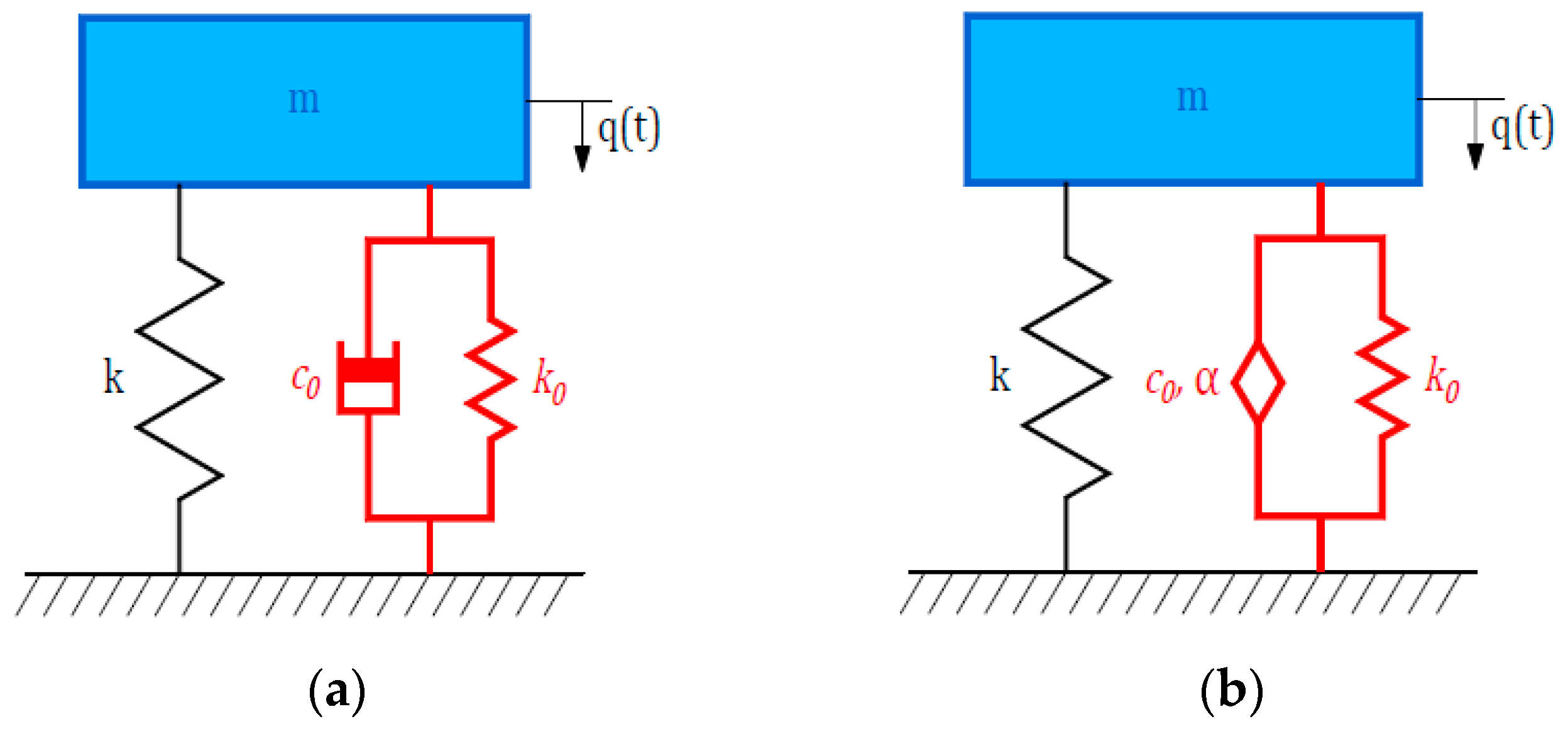
The analysis will focus on viscoelastic models, including both classical and fractional formulations. Figure 1 shows the Kelvin model used in the examples. The classical model is characterized by two parameters associated with stiffness and damping, namely k 0 and c 0 , respectively. In the fractional formulation, the classical dashpot is replaced by a Scott–Blair element, which is additionally described by the parameter α specifying the order of the fractional derivative. A key advantage of fractional models is that they often require fewer parameters to accurately describe material behavior, since they allow a smooth transition between viscous behavior (a first-order derivative) and elastic behavior (a zero-order derivative). Moreover, viscoelastic materials exhibit memory effects, and fractional derivatives provide a natural way to account for history-dependent response. In the present work, the Riemann–Liouville definition is adopted for the fractional model [49]:
D t α x t = d α x t d t α = 1 Γ 1 α d d t 0 t x s t s α d s
where Γ · denotes the Gamma special function.
In this paper, the eigenvalues and the corresponding eigenvectors of Equation (2) are obtained using a continuation method described in detail in [50]. After determining the eigenvalue of mode k in the form:
s k = μ k + i η k
where i = 1 , the natural frequency can be calculated as follows:
ω k = μ k 2 + η k 2

3. Local Sensitivity Analysis Using the Direct Differentiation Method

In analytical approaches, sensitivity measures are given by derivatives of the quantities of interest (e.g., natural frequencies) with respect to the design parameters. A detailed presentation of first- and second-order procedures is provided in [19,20]. The latter work also includes practical guidelines on when to use a particular sensitivity-analysis variant. Below, the key relations enabling the computation of these sensitivities by direct differentiation are presented. All formulas given below refer to mode k ; however, for the sake of notational simplicity, the subscript k on the eigenvalue has been omitted.
Equation (2) can be written in a compact form as follows:
D s q ¯ s = 0
where D s = s 2 M + s C + K + G s . The eigenvectors can be normalized according to:
1 2 q ¯ T D s s q ¯ = 1
The normalization condition in Equation (7) was adopted because it yields a symmetric coefficient matrix in the resulting system, which is advantageous from the numerical point of view.
Differentiation of Equations (6) and (7) with respect to the design parameter p i , and analogously with respect to the pair of design parameters p i and p j , leads to the following compact system for the first- and second-order sensitivities:
D s D s s q ¯ q ¯ T D s s 1 2 q ¯ T 2 D s s 2 q ¯ q , β s . β = h 1 , β h 2 , β
where the subscript β denotes differentiation with respect to design parameters. In particular, for first-order sensitivities, β = i , so that q , i = q ¯ / p i and s , i = s / p i . For second-order sensitivities, β = i i denotes differentiation twice with respect to p i , whereas β = i j denotes mixed differentiation with respect to p i and p j , i.e., q , i j = 2 q ¯ / p i p j , s , i j = 2 s / p i p j . The explicit expressions for the right-hand-side terms h 1 , β and h 2 , β are given in Appendix A.
If the eigenvalue sensitivities are expressed as follows:
s p i = μ p i + i η p i
for the first-order sensitivity, and
2 s p i p j = 2 μ p i p j + i 2 η p i p j
for the second-order sensitivity, then the sensitivities of the natural frequency can be computed as follows:
ω p i = 1 ω μ μ p i + η η p i
2 ω p i p j = 1 ω μ p i μ p j + η p i η p j + μ 2 μ p i p j + η 2 η p i p j ω p i ω p j
Detailed derivatives for various rheological models were provided in [19]. The presented formulas allow one to determine sensitivity measures; however, it should be emphasized that they are local in nature, i.e., they are evaluated at the nominal point p 0 and describe the system response to small parameter perturbations in its immediate vicinity. Therefore, the interpretation of the results depends on the choice of p 0 and may change when a different reference point is adopted. First-order sensitivities describe the direct rate of change in the response with respect to the design parameters. In turn, second-order sensitivities provide information about the curvature of this dependence, and are therefore particularly useful for identifying nonlinear parameter effects.
Local sensitivities can be used to rank parameters from an engineering perspective. To compare the influence of different parameters on the natural frequency, a dimensionless sensitivity measure is defined as follows:
S p = p ω ω p
A larger value of S p indicates a stronger influence of the parameter p on the response. The sign of S p determines the direction of change: S p > 0 means that an increase in p increases ω , whereas S p < 0 implies the opposite. In particular, for a small relative perturbation Δ p / p , the corresponding relative change in the response can be approximated as Δ ω / ω S p   Δ p / p . Thus, if S p = h , then a 1% increase in p leads approximately to an h % change in ω .

4. Machine-Learning Approaches to Modal Sensitivity Analysis

4.1. Training Data Generation

Data for the models under consideration were generated numerically based on the assumed input data. Based on the data sets generated during sampling, the model’s dynamic response corresponding to the assumed data was computed. Two methods of generating samples were used, Latin Hypercube Sampling (LHS) and Grid Sampling (GS).
For sets generated by the LHS method, the ranges of individual parameters were divided evenly into a defined number of samples, and then a random permutation of the set was performed for each parameter. Data sets for calculations were created in a way that excludes the multiple use of a selected parameter value. The number of samples specified during the division is also the number of computational combinations that can be generated.
In GS, parameter ranges are divided evenly into a defined number of samples, and then all possible combinations between individual parameters are generated. The number of data sets for this generation method is J N , where J is the number of samples of individual parameters, whereas N is the number of parameters characterizing the analyzed system.
The next step was data standardization. The input data, i.e., the values of the system parameters, were standardized, whereas the output data were not standardized. Moreover, a separate surrogate model was trained for each considered mode, which reduced the influence of possible scale differences across modes.
For the examples presented in the next section, the number of generated samples was determined by the need to obtain a properly trained model while maintaining optimal computational time. The number of generated samples varied depending on the model being analyzed and, within individual models, depending on the method used to generate the datasets for the computations.

4.2. Surrogate Modeling of Natural Frequencies

Two surrogate models were used in the analyzed examples: Multi-layer Perceptron Regressor (MLPR) and Gaussian Process Regressor (GPR). In the present study, the surrogate models were trained to predict the real natural frequencies, since the main objective was to assess the applicability of machine learning-based models to sensitivity analysis of natural frequencies and to parameter ranking. The MLPR network is trained by minimizing the squared error as the loss function, with a linear output layer, that is, without an activation function in the output layer. For this type of network, the possibility of using two optimizers was analyzed. The first is the “lbfgs” optimizer from the family of quasi-Newton methods, while the second is the “Adam” optimizer, which is a stochastic gradient-based method. In the case of MLPR-based networks, hyperparameter tuning was performed using GridSearchCV, taking into account the maximum number of iterations, the value of the parameter α (describing the strength of the regularization term), the choice of the activation function (the tanh function described by the formula f x = tanh   ( x ) or the logistic function according to the formula f x = 1 / ( 1 + exp x ) ), and the hidden-layer size. In all cases, the data were divided into training and test subsets using a fixed random seed, and cross-validation was applied during hyperparameter selection.
The GPR model is based on the concept of a Gaussian process, that is, a collection of random variables such that any finite subset has a joint Gaussian distribution. For the GPR surrogates, a kernel of the form ConstantKernel multiplied by RBF was adopted. The kernel hyperparameters were optimized during model fitting using the standard procedure implemented in scikit-learn, based on the “l-bfgs-b” algorithm, with multiple optimizer restarts and response normalization applied to improve the robustness of the fit. The optimal GPR hyperparameters varied depending on the considered model, sampling strategy, and output quantity. However, in all analyzed case studies, the GPR surrogate provided the highest predictive accuracy and was therefore selected as the preferred surrogate model for further sensitivity analyses. A summary of the dataset sizes, train/test splits, and representative surrogate-model settings is given in Table 1.

4.3. Machine Learning-Based Sensitivity Methods

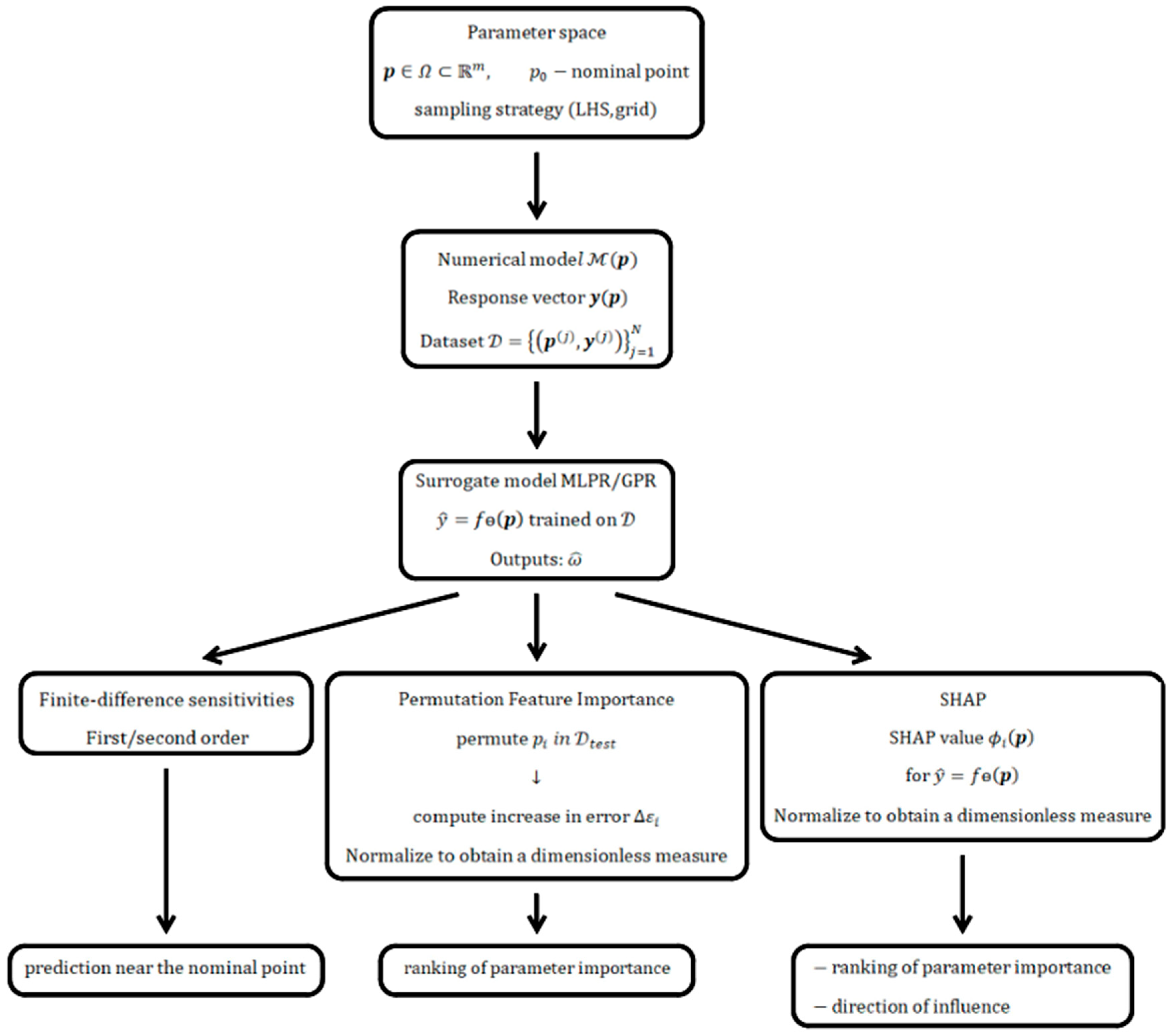
To link the proposed metamodeling approach with classical derivative-based sensitivity analysis, two complementary groups of ML-based measures are considered. First, local sensitivities of the natural frequencies are extracted from the surrogate models using finite differences evaluated in the vicinity of the nominal point.
Second, to enable an importance ranking of parameters that is consistent across different parameter scales, feature-importance measures are employed. In particular, permutation feature importance and Shapley Additive Explanations are computed for the trained surrogates, and their outputs are reported in a dimensionless form. The resulting rankings are then compared with the dimensionless sensitivity measure S p derived from local sensitivities. The dimensionless sensitivity measure refers to the response variation in the vicinity of the nominal point, whereas SHAP and PFI describe the importance of the parameters over the range covered by the analyzed data. Therefore, it should be kept in mind that the range of variation in the analyzed parameters affects the outcome of the comparison.
The overall workflow and the use of the ML-based algorithms are schematically summarized in Figure 2.

4.3.1. Finite-Difference Estimation of Local Sensitivities from Surrogate Models

Local sensitivities can be extracted from the trained surrogate model ω ^ = ω ^ ( p ) by evaluating finite-difference approximations in the vicinity of the nominal point. Let Δ p i > 0 be a prescribed perturbation step.
The first-order derivative of the natural frequency with respect to parameter p i is approximated using the central difference scheme:
ω p i p 0 = ω ^ p 0 + p i ω ^ p 0 p i 2 p i
The second-order derivative with respect to parameter p i is computed as (for p i = p j ) :
2 ω p i 2 p 0 = ω ^ p 0 + p i 2 ω ^ ( p 0 ) + ω ^ p 0 p i p i 2
The perturbation step is selected as a relative fraction of the nominal parameter value Δ p i = δ   p 0 , i .

4.3.2. Permutation Feature Importance-Based Sensitivity Analysis

Permutation feature importance relies on the use of a surrogate model trained on complete, structured input and output data. The model’s baseline mean square error (RMSE) is calculated for the surrogate predictions, relating it to the reference values obtained in the analytical method, using the following formula:
R M S E b a s e = 1 N i = 1 N ω i m m ω i 2
where N is the number of samples used to compute the error, ω i m m denotes the natural frequency predicted by the surrogate model for the i -th sample and ω i is the corresponding reference value obtained from solving the governing model for the same input parameters.
In the next step, a random permutation of one of the input parameters is performed to break the link between the parameter and the model response and generate new predictions (without retraining the model) [39]. For these predictions, the mean squared error is calculated again with respect to the reference values. The effect of permuting the parameter on the resulting model response can be calculated as follows:
R M S E i = R M S E p e r m , i R M S E b a s e
where R M S E p e r m , i is the root mean squared error computed after permuting the i -th input parameter in the validation set.
After normalization according to the formula below:
S P E R i = R M S E i j R M S E j
The result is interpreted as the dimensionless importance measure of parameter p i .

4.3.3. Shapley Additive Explanations-Based Sensitivity Analysis

The SHAP algorithm allows us to determine the extent to which each parameter influences the model response using the predictions of a trained surrogate model [51]. The algorithm determines the influence of individual parameters based on the weighted average of the differences in the model predictions obtained for subsets that include parameter i and the corresponding subsets that exclude this parameter. The SHAP value is defined as follows:
ϕ i = S P \ p i S ! P S 1 ) ! P ! f S p i x S p i f s x s
where ϕ i denotes the SHAP value associated with parameter p i , P is the set of all input parameters and P is the number of parameters, S denotes a subset of parameters that does not include parameter p i and S denotes the cardinality of S , f S ( · ) denotes the model prediction evaluated using only the parameters in subset S , and x S is the corresponding subvector of the input x .
By calculating the mean absolute value of ϕ i   over N samples, a global importance measure for a given model is obtained:
J i = 1 N n = 1 N ϕ i p n
where N is the number of samples used to compute the average, ϕ i ( p n ) is the SHAP value of parameter i computed for the n -th input sample, p n denotes the input vector of model parameters for the n -th sample.
After normalization by the sum over features, a dimensionless measure is obtained:
S S H i = J i j J j
The SHAP algorithm allows the impact of features on the model response to be evaluated in terms of both positive and negative contributions.

5. Examples

5.1. Single-Degree-of-Freedom System

In Section 5.1, a single-degree-of-freedom system shown in Figure 3 is analyzed. A comparison between the results obtained from the analytical solution and those obtained using machine learning was performed for two Kelvin-type models: the classical Kelvin model and the fractional Kelvin model (Figure 1). The following nominal parameter values were assumed: mass m = 10   k g , structural stiffness k k = 1000   N / m , damping coefficient of the damping element c 0 = 20   N s α / m , spring stiffness in the damping element k 0 = 500   N / m , and, in the case of the fractional model, the fractional derivative order α = 0.8 . In this example, the natural frequency ω is analyzed. For the nominal parameter values, the natural frequency for the classical Kelvin model equals 12.2474 rad/s, whereas for the fractional Kelvin model it equals 12.4412 rad/s.

5.1.1. Comparison of Sensitivity Values for Different Metamodels

Table 1, Table 2, Table 3 and Table 4 present a comparison of the first-order sensitivities computed analytically using Formulas (11) and (12), and the sensitivities determined from the metamodels using Formulas (14) and (15). The classical and fractional Kelvin models were analyzed assuming 5% variation in each parameter around its nominal value. Two parameter-space sampling strategies were employed: Grid Sampling and Latin Hypercube Sampling. In each case, three approximation approaches were used: MLPR-lbfgs, MLPR-Adam, and GPR-lbfgs. The sensitivities based on the metamodels were computed using a perturbation value of Δ p = 0.01 p . Table 2 and Table 3 present the results for the classical model, while Table 4 and Table 5 correspond to the fractional model.
The comparison of the analytical results with the derivatives obtained from the metamodels shows that the best agreement is achieved by GPR-lbfgs, which accurately reproduces all derivative values. The MLPR models also yield correct results; however, they exhibit larger deviations. In particular, for MLPR in the case of the classical Kelvin model, small non-zero sensitivity values are observed for c 0 , although variations of c 0 do not affect the analyzed structural response. These non-zero values are attributed to approximation errors of the metamodel and numerical noise, which may produce spurious derivatives for parameters with no true influence on the response.
Comparing the obtained results with respect to the choice of sampling strategy for both the classical and fractional models, it can be observed that, in the case of a well-fitted metamodel (GPR), both sampling approaches lead to very similar results. This indicates that, when an accurate metamodel is used, the influence of the sampling strategy on the final sensitivity results becomes secondary. For second-order derivatives, the differences between the metamodels are more pronounced, and in practice, only GPR-lbfgs provides good agreement with the analytical solution. Table 6 presents the results for the fractional model obtained using GPR-lbfgs, which will also be employed in the subsequent analyses. Grid Sampling was applied.

5.1.2. Analysis of the Effect of the Perturbation Step on Sensitivity Values

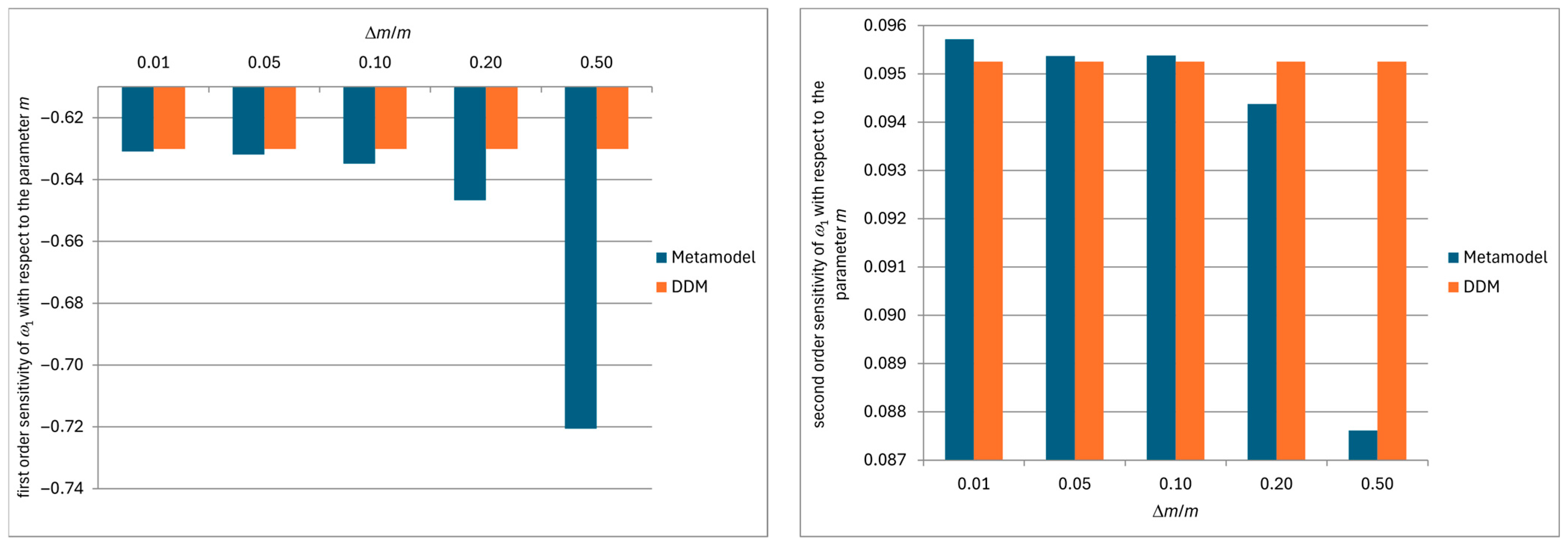
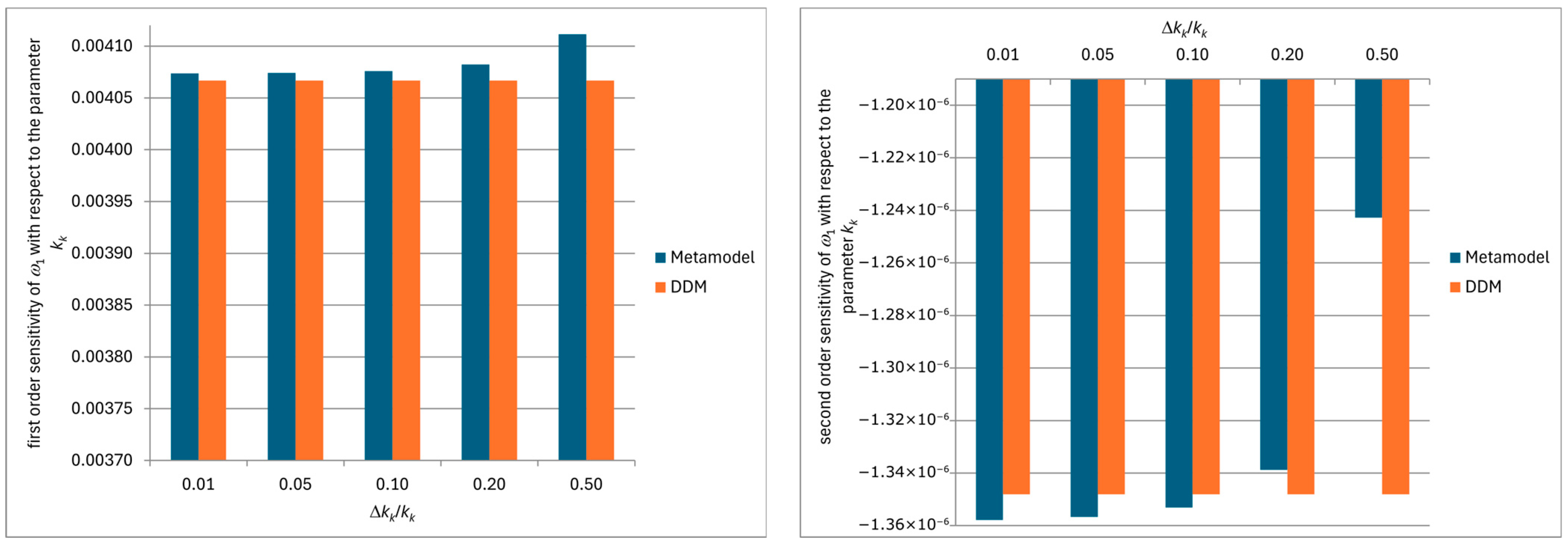
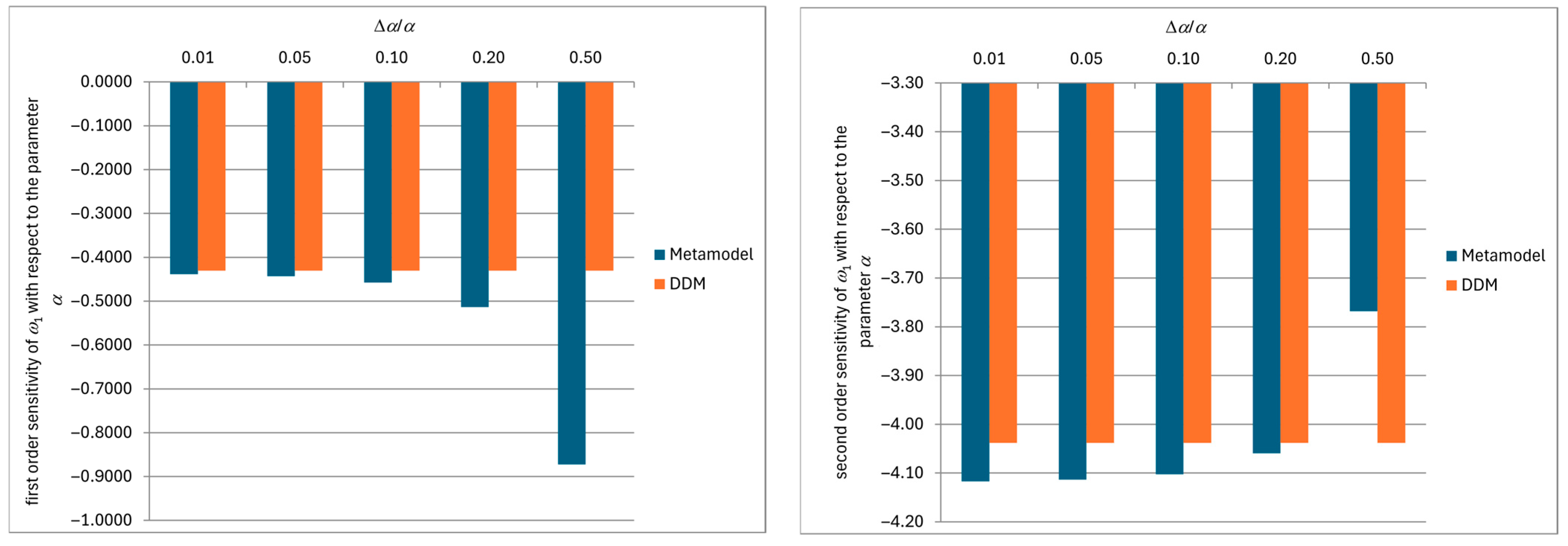
For the fractional model, an analysis was performed to investigate the influence of the perturbation step Δ p . The results are presented in the form of plots (Figure 4, Figure 5 and Figure 6) for a parameter with a strong influence—mass m , for a parameter with a moderate influence—stiffness ( k k ), and for a parameter whose influence on the system response is strongly nonlinear—order of fractional derivative α . The GPR-lbfgs metamodel was used, assuming 5% parameter uncertainty around nominal values and employing the Grid Sampling strategy.
Figure 4, Figure 5 and Figure 6 show that for small perturbation steps Δ p , the agreement between the sensitivities obtained from the surrogate model and those computed analytically is very good. As Δ p increases, the finite-difference approximation becomes less accurate, and consequently, the discrepancies between the surrogate-based and analytical results also increase. Similar conclusions can be drawn for all analyzed parameters, including the parameter α , which exhibits stronger local nonlinearity. The performed analyses indicate that an appropriate choice of Δ p is crucial for achieving good agreement; therefore, it is necessary to carry out computations for several perturbation levels to test the stability of the solution.

5.1.3. Analysis of the Influence of Parameter Dispersion on Sensitivity Values

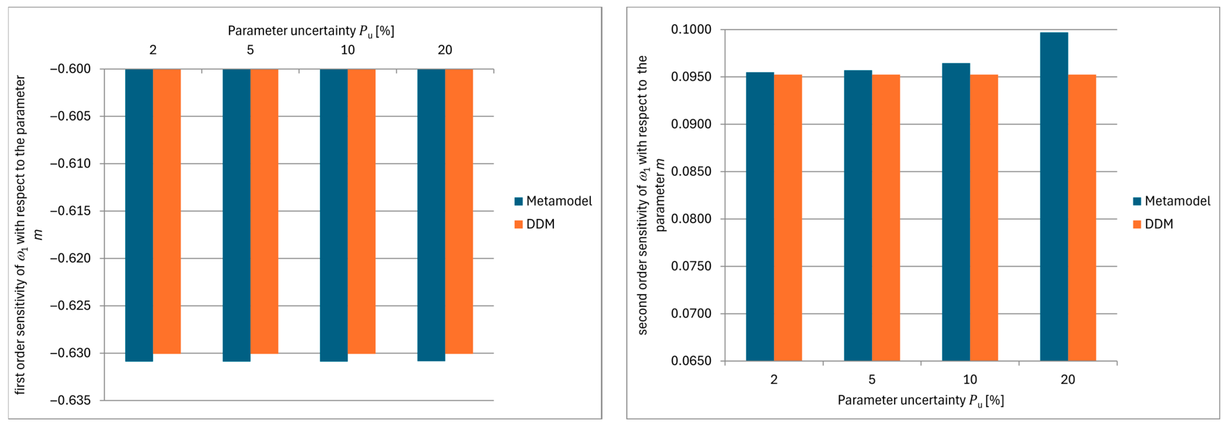
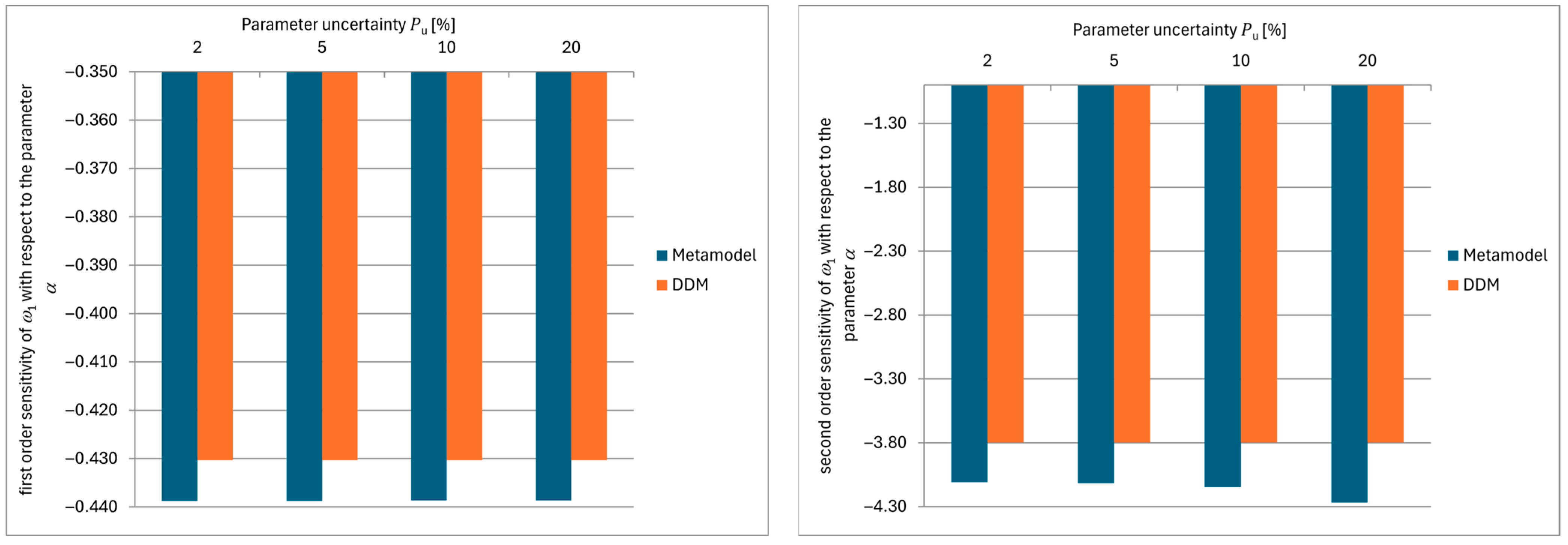
An analysis of the variation in parameter dispersion was performed in order to assess the stability of the obtained sensitivity values. Parameter dispersion levels ( P u ) of 2%, 5%, 10%, and 20% around nominal values were considered for comparison. The obtained results are presented in the form of plots (Figure 7 and Figure 8). The results are shown for two selected parameters of the fractional model: m and α. The GPR-lbfgs metamodel was employed with a perturbation step of Δ p = 0.01 p and the Grid Sampling strategy.
Figure 7 and Figure 8 indicate that increasing the uncertainty level does not significantly affect the results obtained using the surrogate model. Minor differences can be observed for the second-order sensitivities. It can be concluded that, for the analyzed system, local sensitivities, especially the first-order ones, are robust with respect to changes in the assumed dispersion level. Nevertheless, it is advisable to verify the stability of the results with respect to P u .
It should be noted, however, that the limited influence of parameter dispersion observed here is related to the analyzed example, and for strongly nonlinear or higher-dimensional systems, this effect may require separate investigation.

5.1.4. Comparison of Feature Importance Measures

Dimensionless sensitivities were also computed using Formula (13) based on the analytically derived sensitivities. The obtained quantities can be used for feature ranking. The results were compared with feature importance measures obtained using the SHAP method and PFI. Table 7 presents the results for the fractional model obtained using Grid Sampling and the GPR-lbfgs metamodel.
The comparison of the dimensionless sensitivity S p with the SHAP and PFI measures lead to consistent qualitative conclusions. The dimensionless sensitivity provides a stable ranking m > k k > k 0 > α > c 0 , and both SHAP and PFI methods reproduce these findings.

5.1.5. Analysis of the Influence of Parameter Dispersion on Feature Importance Measures

The influence of parameter dispersion on the values of feature importance measures was analyzed. The GPR-lbfgs metamodel was employed, considering dispersion levels of 2%, 5%, 10%, and 20% around nominal values. The results for the fractional Kelvin model are summarized in Table 8. The parameter values are the same as in the previous analyses.
Increasing the parameter dispersion P u has only a minor effect on the relative contributions of most parameters in the fractional model. The importance measures for the mass and stiffness parameters remain nearly unchanged. A more noticeable variation is observed only for the fractional derivative order α , and to a lesser extent for c 0 . Despite these quantitative changes, the qualitative ranking of parameter importance remains consistent across all considered dispersion levels.

5.1.6. Assessment of Surrogate Model Robustness to Limited and Noisy Training Data

As an additional test, the influence of training-data quality on the performance of the surrogate models was assessed for the analyzed example with a damper described by a fractional model. Two aspects were considered: a reduction in the size of the training set and the addition of noise to the training data.
In the case of reducing the size of the training set, the predictive performance of all analyzed surrogate models remained very good. For the MLP-lbfgs model, the test R 2 values ranged from 0.999491 to 0.999900 when the training set was reduced from 100% to 20% of its original size. For the MLP-Adam model, the corresponding test R 2 values ranged from 0.999083 to 0.999554. The GPR model also maintained very high predictive accuracy for all analyzed training-set sizes, with the test R 2 value remaining equal to 1.0 even when the dataset was reduced to 20% of its initial size. These results indicate that, for the analyzed benchmark, a moderate reduction in the number of training samples did not lead to a significant deterioration in the predictive quality of the surrogate models.
In the case of noisy training data, a gradual deterioration in predictive accuracy was observed for both MLP-based models as the noise level increased. For MLP-lbfgs, the test R 2 value decreased from 0.999663 for the noise-free case to 0.999639, 0.998905, and 0.994914 for noise levels of 0.5%, 1%, and 2%, respectively. For the MLP-Adam model, the corresponding values were 0.999554, 0.999531, 0.999315, and 0.997973. For the GPR model, the addition of noise led to a much stronger deterioration in predictive performance. Moreover, preliminary calculations indicated that the GPR-based surrogate may already exhibit unstable behavior for the 0.5% noise level, depending on the particular realization of the random perturbation. Therefore, in contrast to the MLP-based models, the GPR surrogate appeared to be markedly less robust with respect to noisy training data. Detailed results are presented in Table 9 and Table 10.
For the analyzed benchmark, reducing the size of the training set did not significantly affect the predictive quality of the surrogate models. The first-order sensitivities remained in good agreement with the analytical results for the MLP-based models, whereas for the GPR model, the second-order sensitivities were also reproduced accurately. In contrast, the addition of noise led to a clear deterioration in both predictive accuracy and the agreement between the sensitivities determined from the surrogate models and the analytical results. This effect was particularly pronounced for the GPR model, which proved to be not only more sensitive to noisy training data but also less stable, since the obtained results depended substantially on the particular realization of the random perturbation. It should be emphasized, however, that this analysis is preliminary and was carried out for only one representative example. A more systematic investigation of surrogate model-based sensitivity analysis in the case of incomplete and noisy data will be the subject of future research.

5.2. Frame Structure with Viscoelastic Damper

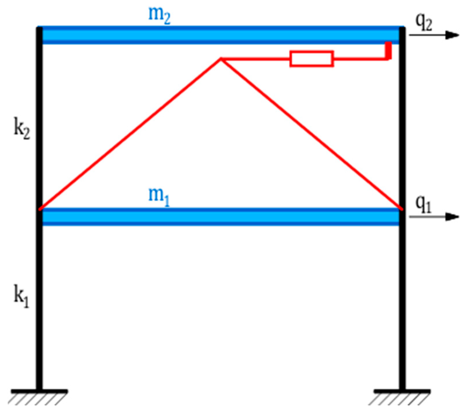
In Section 5.2, a two-story frame shown in Figure 9 is analyzed. The structural parameters were assumed as follows: floor masses m 1 = m 2 = 1000 kg and story stiffnesses k 1 = k 2 = 100,000 N/m. The damper behavior is described by a fractional Kelvin model with the following parameters: spring stiffness k 0 = 20,000 N/m, damping coefficient c 0 = 6000 N s α /m, and fractional derivative order α = 0.8 . For the analyses, the GPR-lbfgs metamodel with Grid Sampling was adopted, as it provided the best agreement with the analytical solutions in the single-degree-of-freedom case. Sensitivity values for all parameters and feature importance measures were compared for different damping coefficients. For the nominal parameter values, the natural frequencies are: ω 1 = 6.3954   r a d / s and ω 2 = 18.4440   r a d / s .

5.2.1. Comparison of Sensitivity Values for Different Damping Ratios

A comparison was performed between analytically computed sensitivities and those obtained from the metamodel for different damping levels. By varying the damping coefficient c 0 of the damper, analyses were carried out for nondimensional damping ratios of 0.01, 0.02, and 0.04. A perturbation step of Δ p = 0.01 p and a parameter dispersion of 5% were assumed. Table 11 and Table 12 present the results for the first mode, including first- and second-order sensitivities. Sensitivity values computed analytically are denoted in the tables by the subscript an, whereas those obtained from the metamodel are denoted by the subscript mm.
The obtained results indicate very good agreement between the analytically determined sensitivities and those obtained from the surrogate model. For all analyzed damping levels, the differences between the local sensitivity values are small. This confirms the high accuracy of the applied surrogate model also under variations in the damping parameters. A more pronounced discrepancy was observed only for the second-order sensitivity with respect to k 0 ; however, the absolute error remains very small in this case. Moreover, the influence of k 0 decreases as the damping ratio increases, which may contribute to minor numerical inaccuracies for this parameter.
Particular attention should be paid to the parameter α , whose influence exhibits a clearly nonlinear character. The first-order sensitivities with respect to α change not only in magnitude but, in the case of the first natural frequency, also in sign. This nonlinearity is even more pronounced in the second-order derivatives, whose values for α reach orders of magnitude significantly larger than those for the remaining parameters and strongly depend on the damping level. This indicates that the relationship ω ( α ) is characterized by substantial curvature and a non-uniform rate of change within the analyzed range.
Despite this strongly nonlinear behavior of the parameter α , the metamodel maintains very good agreement with the analytical solution for both first- and second-order sensitivities. This demonstrates its ability to accurately reproduce even complex nonlinear dependencies of the dynamic response on parameters describing fractional damping.

5.2.2. Analysis of Feature Importance Measures for Different Damping Levels

The values of the dimensionless sensitivity were also compared with the results obtained using the PFI and SHAP algorithms. The comparison was performed for the first mode, assuming 5% parameter uncertainty and different damping levels (Table 13).
The obtained results indicate very good agreement between the dimensionless sensitivity S p and the feature importance measures determined using the PFI and SHAP methods for all analyzed damping levels. This confirms the reliability of the metamodel-based sensitivity analysis. An important conclusion is that the metamodel correctly reproduces the change in the distribution of parameter importance as the damping level increases, even in situations where the role of a parameter, such as α , undergoes significant changes. This demonstrates the capability of the adopted approach to reliably assess parameter influence also under varying damping levels and partially nonlinear dependencies of the system response on damping-related parameters.
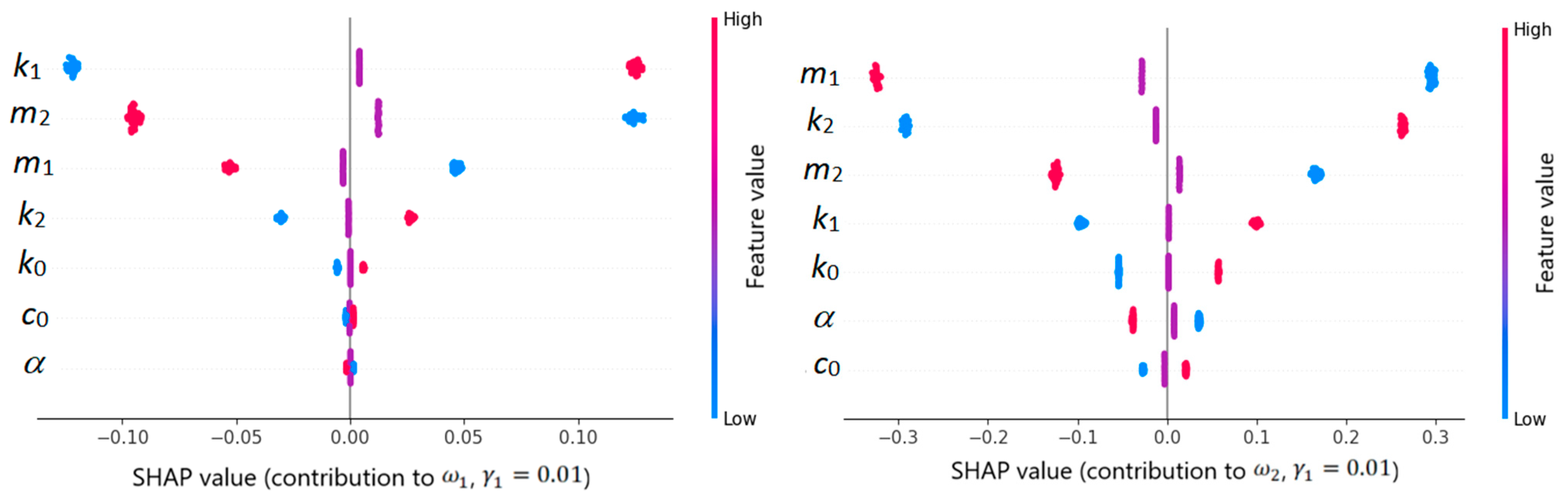
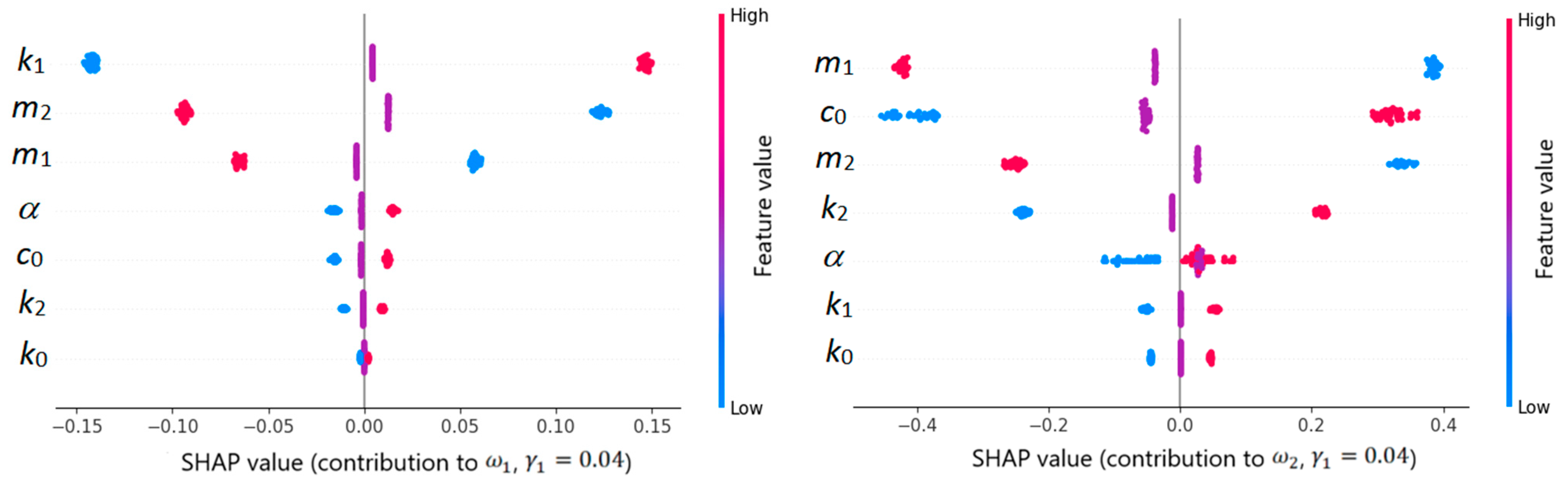
The SHAP algorithm also enables graphical illustration of the distribution of parameter influence. Figure 10 and Figure 11 present the influence of the parameters on the first and second modes for damping ratios of 0.01 and 0.04. On the horizontal axis, SHAP values are shown, interpreted as the contribution of a given parameter to the model response, while the color of the points indicates the parameter value (blue—low, red—high). For a low damping level ( γ = 0.01 ), the first natural frequency is primarily influenced by the story stiffness k 1 and the masses m 2 and m 1 . The parameters directly related to the viscoelastic damper, i.e., c 0 and the fractional derivative order α , exhibit only a minor influence in this case. As the damping level increases ( γ = 0.04 ), a clear change in the distribution of parameter importance is observed. The influence of the damping coefficient c 0 , and particularly of the parameter α , increases significantly, indicating that the dynamic response of the structure becomes increasingly governed by the damping mechanism. For the second natural frequency, the contribution of damping-related parameters also becomes more pronounced at the higher damping level, especially in the case of c 0 , although the mass and stiffness parameters still play a major role.
An important additional advantage of SHAP analysis is the ability to determine not only the magnitude but also the direction of parameter influence on the structural response. The sign of the SHAP value indicates whether an increase in a parameter leads to an increase or a decrease in the analyzed natural frequency. For example, for stiffness parameters, high values (marked in red) shift towards positive SHAP values, corresponding to an increase in frequency, whereas for masses, high parameter values lead to negative contributions, i.e., a decrease in frequency.

5.2.3. Sensitivity Analysis at a Shifted Nominal Point

An additional analysis was performed for a shifted reference point. The previously trained GPR-lbfgs metamodel was used for the computations, without retraining. The reference point was shifted by increasing all parameters by 2% relative to their nominal values, while maintaining the perturbation step Δ p = 0.01 p . First- and second-order sensitivity results obtained analytically for the shifted nominal point, as well as those computed from the metamodel, are presented in Table 14 and Table 15.
The obtained results indicate that shifting the reference point does not lead to significant differences between the analytical results and those obtained from the metamodel. These results confirm that the applied metamodel correctly reproduces the local properties of the response, also beyond the originally assumed nominal point. This constitutes an important advantage of the proposed approach, since in analytical methods, a change in the nominal point requires the problem to be solved again.

6. Conclusions

This paper presented a machine learning-based framework for modal sensitivity analysis of systems with viscoelastic damping elements, considering both classical and fractional rheological models. The proposed framework demonstrates the use of machine learning to estimate both local sensitivities of natural frequencies and a parameter-importance ranking. The ranking obtained from PFI and SHAP is compared with the dimensionless sensitivity measure, while the surrogate-based local sensitivities computed by finite differences are validated against analytically derived results based on the direct differentiation method. Two representative examples are investigated: a single-degree-of-freedom oscillator with classical and fractional Kelvin damper, and a two-story frame equipped with a fractional Kelvin damper. This combination of examples enables the following conclusions to be drawn regarding the proposed approach and its application to systems with viscoelastic elements:
  • A very good agreement was obtained between the first- and second-order local sensitivities computed using the surrogate model and those computed analytically. Good agreement requires the use of an appropriately selected surrogate model.
  • For systems with viscoelastic elements, GPR proved to be the most reliable surrogate model. MLP-based surrogates reproduced similar tendencies, but the results differed slightly from those obtained analytically, and for parameters with negligible influence, nonzero sensitivities appeared in the results.
  • The choice of the perturbation step Δ p used to compute sensitivities from the surrogate model is important. The presented examples show that increasing Δ p reduced the agreement with the analytical results, particularly for the parameter α , which has a strongly nonlinear influence. Therefore, when applying the proposed approach, it is essential to examine the stability of the sensitivities with respect to Δ p .
  • No significant effect of parameter dispersion on the qualitative conclusions of the conducted analyses was observed.
  • Good agreement was obtained between the feature-importance measures and the rankings based on analytical derivatives. After normalization, the PFI and SHAP algorithms produced results very similar to those obtained with the dimensionless sensitivity measure. This indicates that ML-based feature-importance algorithms can reliably provide information on parameter ranking for systems with viscoelastic damping.
  • The proposed machine learning-based approach makes it possible to accurately reproduce the values of local sensitivities and feature-importance measures for different damping levels. The conducted analyses showed that, even for higher damping, the agreement between the ML-based approach and the analytical results remained very good.
  • It was also demonstrated that the proposed approach enables accurate sensitivity results even when the original nominal point is shifted. Using the previously trained surrogate model, very good agreement of the sensitivity values with those obtained analytically was achieved. This can be achieved without retraining, provided that the shifted nominal point remains within the parameter domain covered by the training data. This is a practical advantage of the ML-based approach, since in analytical methods, the sensitivities must be recomputed when the nominal point changes.
  • From the computational point of view, the preparation of the training data and the surrogate model training require an additional effort, but once the surrogate is available, repeated evaluations of the response and the corresponding sensitivity estimates can be obtained very efficiently. Therefore, the approach is particularly attractive in applications involving repeated analyses, such as parametric studies, uncertainty quantification, optimization, or sensitivity assessment for shifted nominal points. A systematic comparison of computational times for large-scale FEM-based systems will be addressed in future work.
  • The present study also has some limitations. The proposed framework was tested on relatively simple benchmark systems, and, therefore, its effectiveness for more complex structures requires further investigation. No direct experimental validation of the proposed machine-learning-based approach was carried out. However, the obtained results were compared with analytical solutions known from the literature.
The results show that machine-learning-based surrogate models reproduce sensitivity measures with good accuracy and remain consistent with the analytical results. This indicates that such an approach can be successfully used in sensitivity analysis, while the reduction in computational effort constitutes an additional practical advantage.

Author Contributions

Conceptualization, M.Ł.-P.; methodology, J.P. and M.Ł.-P.; software, J.P. and M.Ł.-P.; validation, J.P. and M.Ł.-P.; formal analysis, J.P. and M.Ł.-P.; investigation, J.P. and M.Ł.-P.; resources, J.P. and M.Ł.-P.; data curation, J.P. and M.Ł.-P.; writing—original draft preparation, J.P. and M.Ł.-P.; writing—review and editing, J.P. and M.Ł.-P.; visualization, J.P. and M.Ł.-P.; supervision, M.Ł.-P.; project administration, M.Ł.-P.; funding acquisition, M.Ł.-P. All authors have read and agreed to the published version of the manuscript.

Funding

This research was funded by the research project of Poznan University of Technology, grant number 0411/SBSD/0014.

Institutional Review Board Statement

Not applicable.

Informed Consent Statement

Not applicable.

Data Availability Statement

The data presented in this article and the codes used are available upon request to the corresponding author.

Conflicts of Interest

The authors declare no conflicts of interest.

Appendix A

This appendix collects the explicit forms of the right-hand-side terms appearing in the systems of equations used to compute the first- and second-order sensitivities:
h 1 , 1 = D s p i q ¯
h 2 , 1 = 1 2 q ¯ T 2 D s p i s q ¯
h 1 , 2 = 2 D s p i p j + 2 D s s 2 s p i s p j + 2 D s s p j s p i + 2 D s s p i s p j q ¯        + D s p i + D s s s p i q ¯ p j + D s p j + D s s s p j q ¯ p i
h 2 , 2 = 1 2 q ¯ T 3 D s s p i p j + 3 D s 3 s s p i + 3 D s 2 s p i s p j + 3 D s 2 s p j s p i q ¯         + q ¯ T 3 D s s p j + 2 D s s 2 s p j q ¯ p i         + q ¯ T 2 D s s p i + 2 D s s 2 s p i q ¯ p j + q T p i D s s q ¯ p j

References

  1. Lewandowski, R.; Baum, M. Dynamic characteristics of multilayered beams with viscoelastic layers described by the fractional Zener model. Arch. Appl. Mech. 2015, 85, 1793–1814. [Google Scholar] [CrossRef]
  2. Lewandowski, R.; Litewka, P.; Wielentejczyk, P. Free vibrations of laminate plates with viscoelastic layers using the refined zig-zag theory. Part 1 Theoretical background. Compos. Struct. 2021, 278, 114547. [Google Scholar] [CrossRef]
  3. Lewandowski, R.; Bartkowiak, A.; Maciejewski, H. Dynamic analysis of frames with viscoelastic dampers: A comparison of damper models. Struct. Eng. Mech. 2012, 41, 113–137. [Google Scholar] [CrossRef]
  4. Yavas, C.; Pawlak, Z.M. Seismic Retrofitting of Reinforced Concrete Frames Using Viscoelastic Layers at Beam–Column Joints. Appl. Sci. 2026, 16, 1712. [Google Scholar] [CrossRef]
  5. Lewandowski, R.; Litewka, P.; Łasecka-Plura, M.; Pawlak, Z.M. Dynamics of structures, frames, and plates with viscoelastic dampers or layers: A literature review. Buildings 2023, 13, 2223. [Google Scholar] [CrossRef]
  6. van Keulen, F.; Haftka, R.T.; Kim, N.H. Review of options for structural design sensitivity analysis. Part 1: Linear systems. Comput. Methods Appl. Mech. Eng. 2005, 194, 3213–3243. [Google Scholar] [CrossRef]
  7. Tortorelli, D.A.; Michaleris, P. Design sensitivity analysis: Overview and review. Inverse Probl. Eng. 1994, 1, 71–105. [Google Scholar] [CrossRef]
  8. Kim, T.W.; Kim, J.H. Eigensensitivity based optima distribution of a viscoelastic damping layer for a flexible beam. J. Sound Vib. 2004, 273, 201–218. [Google Scholar] [CrossRef]
  9. Chen, S.H.; Ma, L.; Meng, G.W.; Guo, R. An efficient method for evaluating the natural frequencies of structures with uncertain-but-bounded parameters. Comput. Struct. 2009, 87, 582–590. [Google Scholar] [CrossRef]
  10. Fox, R.L.; Kapoor, M.P. Rates of change of eigenvalues and eigenvectors. AIAA J. 1968, 6, 2426–2429. [Google Scholar] [CrossRef]
  11. Nelson, R.B. Simplified calculation of eigenvector derivatives. AIAA J. 1976, 14, 1201–1205. [Google Scholar] [CrossRef]
  12. Friswell, M.I.; Adhikari, S. Derivatives of complex eigenvectors using Nelson’s method. AIAA J. 2000, 38, 2355–2357. [Google Scholar] [CrossRef]
  13. Adhikari, S.; Friswell, M.I. Calculation of eigenrelation derivatives for nonviscously damped systems using Nelson’s method. AIAA J. 2006, 44, 1799–1806. [Google Scholar] [CrossRef]
  14. Li, L.; Hu, Y.; Wang, X.; Ling, L. Eigensensitivity analysis of damped systems with distinct and repeated eigenvalues. Finite Elem. Anal. Des. 2013, 72, 21–34. [Google Scholar] [CrossRef]
  15. Li, L.; Hu, Y.J.; Wang, X.L.; Ling, L. Computation of eigensolution derivatives for nonviscously damped systems using the algebraic method. AIAA J. 2012, 50, 2282–2284. [Google Scholar] [CrossRef]
  16. Li, L.; Hu, Y.; Wang, X. A study on design sensitivity analysis for general nonlinear eigenproblems. Mech. Syst. Signal Process. 2013, 34, 88–105. [Google Scholar] [CrossRef]
  17. Lee, T.H. An adjoint variable method for structural design sensitivity analysis of a distinct eigenvalue problem. KSME Int. J. 1999, 13, 470–476. [Google Scholar] [CrossRef]
  18. Lee, T.H. Adjoint method for design sensitivity analysis of multiple eigenvalues and associated eigenvectors. AIAA J. 2007, 45, 1998–2004. [Google Scholar] [CrossRef]
  19. Lewandowski, R.; Łasecka-Plura, M. Design sensitivity analysis of structures with viscoelastic dampers. Comput. Struct. 2016, 164, 95–107. [Google Scholar] [CrossRef]
  20. Łasecka-Plura, M. A comparative study of the sensitivity analysis for systems with viscoelastic elements. Arch. Mech. Eng. 2023, 70, 5–25. [Google Scholar] [CrossRef]
  21. Łasecka-Plura, M. Comprehensive sensitivity analysis of repeated eigenvalues and eigenvectors for structures with viscoelastic elements. Acta Mech. 2024, 235, 5213–5238. [Google Scholar] [CrossRef]
  22. Łasecka-Plura, M.; Lewandowski, R. Dynamic characteristics and frequency response function for frame with dampers with uncertain design parameters. Mech. Based Des. Struct. Mach. 2017, 45, 296–312. [Google Scholar] [CrossRef]
  23. Weber, H. Time-independent stochastic design sensitivity analysis of structural systems with second-order accuracy. J. Theor. Appl. Mech. 2016, 54, 783–794. [Google Scholar] [CrossRef][Green Version]
  24. Guminiak, M.; Kamiński, M.; Lenartowicz, A.; Przychodzki, M. Stochastic vibrations of a system of plates immersed in fluid using a coupled boundary element, finite element, and finite difference methods approach. Materials 2023, 16, 3583. [Google Scholar] [CrossRef]
  25. Reimann, D.; Nidadavolu, K.; ul Hassan, H.; Vajragupta, N.; Glasmachers, T.; Junker, P.; Hartmaier, A. Modeling macroscopic material behavior with machine learning algorithms trained by micromechanical simulations. Front. Mater. 2019, 6, 181. [Google Scholar] [CrossRef]
  26. Aldakheel, F.; Satari, R.; Wriggers, P. Feed-forward neural networks for failure mechanics problems. Appl. Sci. 2021, 11, 6483. [Google Scholar] [CrossRef]
  27. Tabrizikahou, A.; Pavić, G.; Shahsavani, Y.; Hadzima-Nyarko, M. Prediction of reinforced concrete walls shear strength based on soft computing-based techniques. Soft Comput. 2024, 28, 8731–8747. [Google Scholar] [CrossRef]
  28. Prusty, J.K.; Papazafeiropoulos, G.; Mohanty, S.C. Free vibration analysis of sandwich plates with cut-outs: An experimental and numerical study with artificial neural network modelling. Compos. Struct. 2023, 321, 117328. [Google Scholar] [CrossRef]
  29. Seba, M.R.; Kebdani, S. Finite element and neural network based predictive model to determine natural frequency of laminated composite plates with eccentric cutouts under free vibration. Adv. Technol. Innov. 2022, 7, 131–142. [Google Scholar] [CrossRef]
  30. Liu, J.; Yang, X. Learning to see the vibration: A neural network for vibration frequency prediction. Sensors 2018, 18, 2530. [Google Scholar] [CrossRef] [PubMed]
  31. Chakraverty, S.; Singh, V.P.; Sharma, R.K. Regression based weight generation algorithm in neural network for estimation of frequencies of vibrating plates. Comput. Methods Appl. Mech. Eng. 2006, 195, 4194–4202. [Google Scholar] [CrossRef]
  32. Singh, V.P.; Chakraverty, S.; Sharma, R.K.; Sharma, G.K. Modeling vibration frequencies of annular plates by regression based neural network. Appl. Soft Comput. 2009, 9, 439–447. [Google Scholar] [CrossRef]
  33. Dey, S.; Mukhopadhyay, T.; Adhikari, S. Stochastic free vibration analyses of composite shallow doubly curved shells—A Kriging model approach. Compos. Part B Eng. 2015, 70, 99–112. [Google Scholar] [CrossRef]
  34. Dey, S.; Naskar, S.; Mukhopadhyay, T.; Gohs, U.; Spickenheuer, A.; Bittrich, L.; Sriramula, S.; Adhikari, S.; Heinrich, G. Uncertain natural frequency analysis of composite plates including effect of noise—A polynomial neural network approach. Compos. Struct. 2016, 143, 130–142. [Google Scholar] [CrossRef]
  35. Spiridonakos, M.D.; Chatzi, E.N. Metamodeling of dynamic nonlinear structural systems through polynomial chaos NARX models. Compos. Struct. 2015, 157, 99–113. [Google Scholar] [CrossRef]
  36. Denimal, E.; Sinou, J.-J. Advanced kriging-based surrogate modelling and sensitivity analysis for rotordynamics with uncertainties. Eur. J. Mech. A Solids 2021, 90, 104331. [Google Scholar] [CrossRef]
  37. Birrell, M.; Li, Y.; Astroza, R. A Gaussian Process surrogate approach for analyzing parameter uncertainty in mechanics-based structural finite element models. Eng. Struct. 2025, 336, 120435. [Google Scholar] [CrossRef]
  38. Yun, W.; Wang, Y. An efficient Kriging model-based importance sampling method for estimating the failure probability-based parameter global sensitivity index with uncertain distribution parameters. Aerosp. Sci. Technol. 2022, 130, 107861. [Google Scholar] [CrossRef]
  39. Koh, H.; Blum, H.B. Machine learning-based sensitivity of steel frames with highly imbalanced and high-dimensional data. Eng. Struct. 2022, 259, 114126. [Google Scholar] [CrossRef]
  40. Sarkar, N.; Dasgupta, K. Machine learning-based sensitivity analysis of engineering demand parameters for a reinforced concrete wall-frame building. Structures 2024, 70, 107477. [Google Scholar] [CrossRef]
  41. Karathanasopoulos, N.; Singh, A.; Hadjidoukas, P. Machine learning-based modelling, feature importance and Shapley additive explanations analysis of variable-stiffness composite beam structures. Structures 2024, 62, 106206. [Google Scholar] [CrossRef]
  42. Engelbrecht, A.P.; Cloete, I.; Zurada, J.M. Determining the significance of input parameters using sensitivity analysis. In From Natural to Artificial Neural Computation (IWANN 1995); Mira, J., Sandoval, F., Eds.; Lecture Notes in Computer Science; Springer: Berlin/Heidelberg, Germany, 1995; Volume 930, pp. 382–388. [Google Scholar]
  43. Parr, T.; Hamrick, J.; Wilson, J.D. Nonparametric feature impact and importance. Inf. Sci. 2024, 653, 119563. [Google Scholar] [CrossRef]
  44. Burgers, J.M. First and Second Report on Viscosity and Plasticity; Academy of Sciences at Amsterdam: Amsterdam, NY, USA, 1935. [Google Scholar]
  45. Zener, C. Elasticity and Anelasticity of Metals; University of Chicago Press: Chicago, IL, USA, 1948. [Google Scholar]
  46. Renaud, F.; Dion, J.L.; Chevallier, G.; Tawfiq, I.; Lemaire, R. A new identification method of viscoelastic behavior: Application to the generalized Maxwell model. Mech. Syst. Signal Process. 2011, 25, 991–1010. [Google Scholar] [CrossRef]
  47. Bagley, R.L.; Torvik, P.J. Fractional calculus—A different approach to the analysis of viscoelastically damped materials. AIAA J. 1983, 21, 741–748. [Google Scholar] [CrossRef]
  48. Pritz, T. Five-parameter fractional derivative model for polymeric damping materials. J. Sound Vib. 2003, 265, 935–952. [Google Scholar] [CrossRef]
  49. Podlubny, I. Fractional Differential Equation; Academic Press: Cambridge, MA, USA, 1999. [Google Scholar]
  50. Pawlak, Z.; Lewandowski, R. The continuation method for the eigenvalue problem of structures with viscoelastic dampers. Comput. Struct. 2013, 125, 53–61. [Google Scholar] [CrossRef]
  51. Borgonovo, E.; Plischke, E.; Rabitti, G. The many Shapley values for explainable artificial intelligence: A sensitivity analysis perspective. Eur. J. Oper. Res. 2024, 318, 911–926. [Google Scholar] [CrossRef]
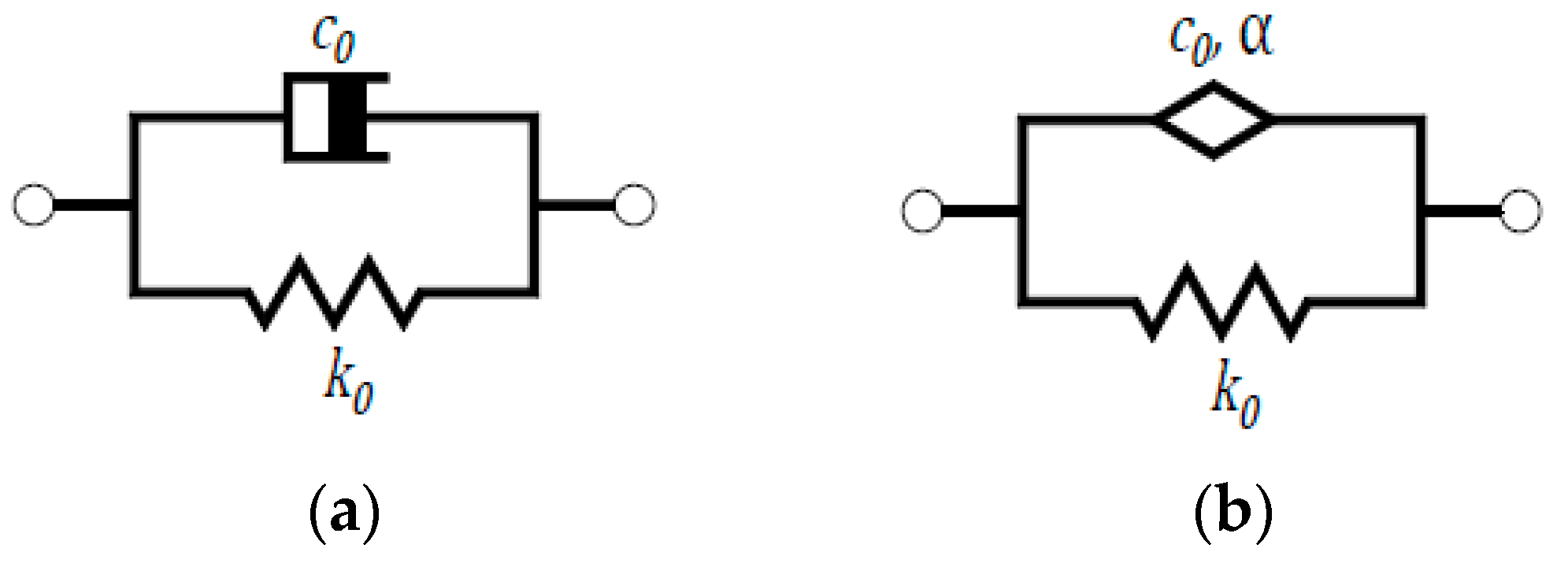
Figure 1. Kelvin model: (a) classical; (b) fractional.
Applsci 16 03749 g001
Figure 2. Framework of the proposed ML-assisted modal sensitivity analysis.
Applsci 16 03749 g002
Figure 3. Single-degree-of-freedom system with a Kelvin damper: (a) classical; (b) fractional.
Applsci 16 03749 g003
Figure 4. First- and second-order sensitivities of ω 1 with respect to m obtained from the metamodel and DDM for different perturbation steps Δ m / m .
Applsci 16 03749 g004
Figure 5. First- and second-order sensitivities of ω 1 with respect to k k obtained from the metamodel and DDM for different perturbation steps Δ k k / k k .
Applsci 16 03749 g005
Figure 6. First- and second-order sensitivities of ω 1 with respect to α obtained from the metamodel and DDM for different perturbation steps Δ α / α .
Applsci 16 03749 g006
Figure 7. First- and second-order sensitivities of ω 1 with respect to m obtained from the metamodel and DDM for different parameter uncertainty levels P u .
Applsci 16 03749 g007
Figure 8. First- and second-order sensitivities of ω 1 with respect to α obtained from the metamodel and DDM for different parameter uncertainty levels P u .
Applsci 16 03749 g008
Figure 9. Frame structure with a fractional Kelvin damper.
Applsci 16 03749 g009
Figure 10. SHAP values for the frame with a fractional Kelvin damper γ 1 0.01 .
Applsci 16 03749 g010
Figure 11. SHAP values for the frame with a fractional Kelvin damper γ 1 0.04 .
Applsci 16 03749 g011
Table 1. Summary of dataset sizes, predictive accuracy, and preferred surrogate models for the analyzed case studies.
Case StudySurrogate ModelNumber of SamplesTrain/Test SplitPreferred Surrogate ModelRepresentative Predictive Accuracy of Preferred Model
SDOF
classical Kelvin model
MLP
(Adam)
129675/25GPR R 2 = 1.0
R M S E = 5.1997 × 10 7
SDOF
classical Kelvin model
MLP
(lbfgs)
129675/25
SDOF
classical Kelvin model
GPR25675/25
SDOF
fractional Kelvin model
MLP
(Adam)
312580/20GPR R 2 = 1.0
  R M S E = 3.03623 × 10 7
SDOF
fractional Kelvin model
MLP
(lbfgs)
312580/20
SDOF
fractional Kelvin model
GPR102475/25
Frame
mode 1
GPR21871800/387GPR R 2 = 1.0
  R M S E = 1.31457 × 10 5
Frame
mode 2
GPR21871800/387GPR R 2 = 1.0
R M S E = 2.88926 × 10 5
Table 2. Comparison of first-order sensitivity values using Grid Sampling—classical Kelvin model.
Parameter
p
UnitParameter Value ω p MLPR-lbfgsMLPR-AdamGPR-lbfgs
mkg10−0.612372−0.622670−0.613647−0.612408
kkN/m10000.0040820.0041710.0040860.004082
k0N/m5000.0040820.0040750.0040870.004082
c0Ns/m200.000000−0.0036380.0002590.000000
Table 3. Comparison of first-order sensitivity values using Latin Hypercube Sampling—classical Kelvin model.
Parameter
p
UnitParameter Value ω p MLPR-lbfgsMLPR-AdamGPR-lbfgs
mkg10−0.612372−0.625982−0.614588−0.612408
kkN/m10000.0040820.0041720.0040840.004082
k0N/m5000.0040820.0038540.0040730.004082
c0Ns/m200.000000−0.0024300.0004830.000000
Table 4. Comparison of first-order sensitivity values using Grid Sampling—fractional Kelvin model.
Parameter
p
UnitParameter Value ω p MLPR-lbfgsMLPR-AdamGPR-lbfgs
mkg10−0.6300765−0.6451346−0.6314510−0.6308961
kkN/m10000.00406690.00416880.00407770.0040736
k0N/m5000.00406690.00422420.00408110.0040736
c0Nsα/m200.01002220.00844840.00982080.0099100
α-0.8−0.4303417−0.4176872−0.4420842−0.4387608
Table 5. Comparison of first-order sensitivity values using Latin Hypercube Sampling—fractional Kelvin model.
Parameter
p
UnitParameter Value ω p MLPR-lbfgsMLPR-AdamGPR-lbfgs
mkg10−0.6300765−0.6377284−0.6317276−0.6308958
kkN/m10000.00406690.00410040.00407730.0040736
k0N/m5000.00406690.00410410.00407690.0040736
c0Nsα/m200.01002220.00991650.00975040.0099096
α-0.8−0.4303417−0.4221428−0.4380069−0.4387665
Table 6. Comparison of second-order sensitivity values—fractional Kelvin model.
Parameter
p
UnitParameter Value 2 ω 2 p GPR-lbfgs
mkg100.09525530.0957185
kkN/m1000−0.0000013−0.0000014
k0N/m500−0.0000013−0.0000014
c0Nsα/m200.00003470.0000229
α-0.8−4.0384941−4.1171190
Table 7. Comparison of feature importance measures using Grid Sampling—fractional Kelvin model.
Parameter
p
UnitParameter
Value
SpGPR-lbfgs
PFISHAP
mkg100.5064390.4728820.475005
kkN/m10000.3268860.3237310.320226
k0N/m5000.1634430.1605480.162950
c0Nsα/m200.0161110.0151750.013774
α-0.80.0276720.0276640.028045
Table 8. Comparison of feature importance measures for different parameter uncertainty ranges—fractional Kelvin model.
Parameter
p
Sp P u = 2 % P u = 5 % P u = 10 % P u = 20 %
PFISHAPPFISHAPPFISHAPPFISHAP
m0.5064390.4729470.4753200.4728820.4750050.4726700.4741350.4716850.470989
kk0.3268860.3238980.3201550.3237310.3202260.3231190.3200660.3205450.318677
k00.1634430.1605980.1629380.1605480.1629500.1603420.1628540.1594260.162214
c00.0161110.0153350.0140510.0151750.0137740.0147530.0130580.0136240.010545
α0.0276720.0272220.0275370.0276640.0280450.0291160.0298880.0347190.037574
Table 9. Predictive performance of surrogate models for reduced training data in a single-degree-of-freedom system with a fractional Kelvin damper.
ModelTest
Performance Metrics
Training-Set Size
100%80%60%40%20%
MLP-lbfgs R 2 0.9996630.9996070.9997470.9999000.999491
RMSE0.0052140.0056290.0045170.0028440.006409
MLP-Adam R 2 0.9995540.9995530.9995490.9995320.999083
RMSE0.0060010.0060040.0060330.0061450.008598
GPR R 2 1.01.01.01.01.0
RMSE0.000000290.000000310.000000340.000000530.0000021
Table 10. Predictive performance of MLP-based surrogate models for noisy training data in a single-degree-of-freedom system with a fractional Kelvin damper.
ModelTest
Performance Metrics
Noise Level
0%0.5%1%2%
MLP-lbfgs R 2 0.9996630.9996390.9989050.994914
RMSE0.0052140.0053960.0093980.020255
MLP-Adam R 2 0.9995540.9995310.9993150.997973
RMSE0.0060010.0061530.0074330.012786
Table 11. Comparison of first-order sensitivities for different nondimensional damping ratios—first natural frequency.
Parameter
p
c 0   =   2650   N s α / m
γ   =   0.01
c 0   =   5760   N s α / m
γ   =   0.02
c 0   =   17,300   N s α / m
γ   =   0.04
ω 1 p a n ω 1 p m m ω 1 p a n ω 1 p m m ω 1 p a n ω 1 p m m
m1−9.9872 × 10⁻⁴−9.9936 × 10⁻⁴−1.0384 × 10⁻³−1.0391 × 10⁻³−1.2328 × 10⁻³−1.2338 × 10⁻³
m2−2.1890 × 10⁻³−2.1916 × 10⁻³−2.1910 × 10⁻³−2.1934 × 10⁻³−2.1656 × 10⁻³−2.1679 × 10⁻³
k12.4783 × 10−52.4809 × 10−52.5501 × 10−52.5529 × 10−52.8831 × 10−52.8863 × 10⁻⁵
k25.6575 × 10−65.6693 × 10−64.9650 × 10−64.9740 × 10−62.0204 × 10−62.0201 × 10⁻⁶
k05.6575 × 10−65.6626 × 10−64.9650 × 10−64.9693 × 10−62.0204 × 10−62.0223 × 10⁻⁶
c01.1612 × 10−51.1616 × 10−51.4479 × 10−51.4491 × 10−51.5771 × 10−51.5780 × 10⁻⁵
α−3.6814 × 10⁻²−3.7065 × 10⁻²−1.4436 × 10⁻²−1.4619 × 10−23.7677 × 10−13.7905 × 10⁻¹
Table 12. Comparison of second-order sensitivities for different nondimensional damping ratios—first natural frequency.
Parameter
p
c 0   =   2650   N s α / m
γ   =   0.01
c 0   =   5760   N s α / m
γ   =   0.02
c 0   =   17,300   N s α / m
γ   =   0.04
2 ω 1 p 2 a n 2 ω 1 p 2 m m 2 ω 1 p 2 a n 2 ω 1 p 2 m m 2 ω 1 p 2 a n 2 ω 1 p 2 m m
m12.6703 × 10−72.6912 × 10−73.0490 × 10−73.0710 × 10−75.2431 × 10−75.2989 × 10⁻⁷
m22.0408 × 10−62.0490 × 10−62.0023 × 10−62.0104 × 10−61.7657 × 10−61.7726 × 10⁻⁶
k1−2.2084 × 10⁻¹⁰−2.2149 × 10⁻¹⁰−2.1722 × 10⁻¹⁰−2.1779 × 10⁻¹⁰−1.9580 × 10⁻¹⁰−1.9620 × 10⁻¹⁰
k2−8.6160 × 10⁻¹¹−8.6454 × 10⁻¹¹−6.9700 × 10⁻¹¹−6.9892 × 10⁻¹¹−5.9084 × 10⁻¹²−5.6469 × 10⁻¹²
k0−8.6160 × 10⁻¹¹−8.7550 × 10⁻¹¹−6.9700 × 10⁻¹¹−7.0689 × 10⁻¹¹−5.9084 × 10⁻¹²−4.1663 × 10⁻¹²
c01.1178 × 10−91.0937 × 10−97.2635 × 10−107.3944 × 10⁻¹⁰−3.3822 × 10⁻¹⁰−3.4959 × 10⁻¹⁰
α−2.6364 × 10⁻¹−2.6529 × 10⁻¹−2.7879 × 10⁻¹−2.7881 × 10−11.29241.3063
Table 13. Comparison of feature importance measures for different nondimensional damping ratios—first natural frequency.
Parameter
p
c 0   =   2650   N s α / m
γ   =   0.01
c 0   =   5760   N s α / m
γ   =   0.02
c 0   =   17,300   N s α / m
γ   =   0.04
SpPFISHAPSpPFISHAPSpPFI SHAP
m10.1572530.1569550.1592250.1624490.1614110.1636650.1873940.1741150.176181
m20.3446640.3328100.3470980.3427700.3295050.3434740.3291950.2963710.307302
k10.3902160.3955950.3817000.3989610.4026700.3992430.4382610.4134280.397382
k20.0890800.0871970.0833800.0776760.0756750.0723200.0307120.0279950.026496
k00.0178160.0178210.0183090.0155350.0154500.0158540.0061420.0056620.005696
c00.0048450.0048960.0053410.0130480.0132970.0144070.0414740.0396270.042662
α0.0046370.0047260.0049460.0018070.0019920.0020390.0458180.0438030.044281
Table 14. Comparison of sensitivity values for a shifted nominal point—first natural frequency.
Parameter
p
UnitParameter Value ω 1 p a n ω 1 p m m 2 ω 1 p 2 a n 2 ω 1 p 2 m m
m1kg1020−1.0212 × 10⁻³−1.0215 × 10−32.9555 × 10−73.1045 × 10⁻⁷
m2kg1020−2.1496 × 10⁻³−2.1509 × 10−31.9224 × 10−62.0068 × 10⁻⁶
k1N/m102,0002.5067 × 10−52.5081 × 10⁻⁵−2.0835 × 10⁻¹⁰−2.1745 × 10⁻¹⁰
k2N/m102,0004.8011 × 10−64.8054 × 10⁻⁶−6.5274 × 10⁻¹¹−6.8455 × 10⁻¹¹
k0N/m20,4004.8011 × 10−64.8031 × 10⁻⁶−6.5274 × 10⁻¹¹−6.9217 × 10⁻¹¹
c0Nsα/m61201.4658 × 10−51.4667 × 10−57.5848 × 10−107.0981 × 10⁻¹⁰
α-0.81−1.4530 × 10⁻²−1.4609 × 10⁻²−2.7772 × 10⁻¹−2.6644 × 10⁻¹
Table 15. Comparison of sensitivity values for a shifted nominal point—second natural frequency.
Parameter
p
UnitParameter Value ω 2 p a n ω 2 p m m 2 ω 2 p 2 a n 2 ω 2 p 2 m m
m1kg1020−6.3130 × 10⁻³−6.3215 × 10−31.1004 × 10−51.1506 × 10⁻⁵
m2kg1020−3.2084 × 10⁻³−3.2136 × 10−36.5432 × 10−66.8368 × 10⁻⁶
k1N/m102,0001.7607 × 10−51.7613 × 10−51.7629 × 10−111.8448 × 10⁻¹¹
k2N/m102,0005.4510 × 10−55.4535 × 10⁻⁵−1.6054 × 10⁻¹⁰−1.6598 × 10⁻¹⁰
k0N/m20,4005.4510 × 10−55.4532 × 10⁻⁵−1.6054 × 10⁻¹⁰−1.6742 × 10⁻¹⁰
c0Nsα/m61202.0325 × 10−42.0316 × 10−41.0752 × 10−81.0596 × 10⁻⁸
α-0.81−2.4565−2.4871−3.1632 × 10⁻¹−2.8792 × 10⁻¹
Disclaimer/Publisher’s Note: The statements, opinions and data contained in all publications are solely those of the individual author(s) and contributor(s) and not of MDPI and/or the editor(s). MDPI and/or the editor(s) disclaim responsibility for any injury to people or property resulting from any ideas, methods, instructions or products referred to in the content.