Precision Micro-Vibration Measurement for Linear Array Imaging via Complex Morlet Wavelet Phase Magnification

Abstract

Traditional vision-based vibration measurement is fundamentally constrained by the low sampling rates of area-scan cameras and the noise sensitivity of existing motion magnification algorithms. To overcome these spatiotemporal barriers, we propose a high-fidelity framework that integrates ultra-high-speed line-scan imaging with a 1D Complex Morlet Wavelet Phase-Based Video Magnification (CMW-PVM) algorithm. By extracting and manipulating the localized phase of 1D spatial signals, CMW-PVM effectively decouples structural dynamics from background noise while eliminating the computational redundancy associated with 2D spatial pyramid methods. Simulations demonstrate that CMW-PVM significantly extends the linear magnification range (up to $\alpha \approx 35$) while preserving exceptional structural fidelity (FSIM $>0.87$) under severe noise conditions (SNR = 10 dB). Experimental validation against a laser Doppler vibrometer (LDV) reveals near-perfect kinematic accuracy, with a relative amplitude error of only 1.65%. Furthermore, at a 100 Hz high-frequency excitation, the system successfully resolves microscopic displacements (≈10 μm) without temporal aliasing—enabled not by violating sampling theory but by leveraging the high physical line rate of the line-scan sensor. This establishes a robust, non-contact, and computationally efficient paradigm for broadband, micro-amplitude vibration monitoring in industrial environments.

1. Introduction

In industrial production, the operational state of critical machinery—such as turbines, generators, and precision manufacturing equipment—is intrinsically linked to subtle vibrational signatures. These micro-vibrations serve as vital indicators of equipment health, early warnings of potential faults (e.g., imbalance, misalignment, and bearing wear), and essential data for structural dynamics analysis [1]. Similarly, in civil engineering, large-scale structures such as bridges, skyscrapers, and offshore platforms undergo continuous, often imperceptible, geometric deformations and vibrations under operational loads (e.g., traffic, wind, waves) and environmental influences [2,3]. Accurately measuring these micro-amplitude, potentially high-frequency vibrations is paramount for structural health monitoring, safety assessment, and predictive maintenance [4].

Traditional non-contact vibration measurement techniques, including laser Doppler vibrometers (LDVs), fiber Bragg grating (FBG) sensors, and photoelectric position sensors [5], offer high precision but often suffer from limitations such as point-based sensing (lacking spatial resolution), complex setups, high costs, and sensitivity to environmental interference. The advent and rapid progress in computer vision have catalyzed the emergence of vision-based vibration measurement as a highly flexible, non-contact, and full-field alternative. Originating from digital photogrammetry, this approach extracts structural motion by tracking image features (e.g., edges, corners, and artificial markers) or analyzing pixel intensity variations across video sequences [6]. Similar comparative studies on image-based vibration extraction have highlighted the sensitivity of feature-based methods to noise and lighting variations [7]. This method boasts significant advantages, including non-invasive measurement, high spatial resolution, applicability to complex geometries (such as beams, shells, and enclosures), and, crucially, the absence of mass-loading effects, making it ideal for delicate or micro-scale structures [8].

Conventional vision-based vibration measurement encounters inherent limitations when applied to micro-amplitude vibrations. These limitations manifest primarily in three key areas: (1) Amplitude Sensitivity Constraint: The spatial resolution of standard area-scan cameras, typically limited by pixel sizes exceeding 1 μm, fundamentally restricts the reliable detection of sub-pixel or nanometer-scale displacements. Overcoming this limitation necessitates sophisticated super-resolution techniques, which are computationally intensive and susceptible to noise amplification. (2) Temporal Bandwidth Limit: The frame rate of area-scan cameras, typically constrained to hundreds or a low number of frames per second, imposes a significant bottleneck on the measurable frequency range. Consequently, capturing high-frequency vibrations requires specialized ultra-high-speed cameras, often entailing prohibitive costs. (3) Computational Burden and Artifact Sensitivity: Full-frame vision methods—including feature tracking [9], optical flow [10], and two-dimensional phase analysis—require the processing of large spatial neighborhoods, which results in substantial computational cost and reduced real-time feasibility. Tracking-based approaches are vulnerable to occlusion, drift, and noise-induced trajectory errors, often producing visual artifacts such as “ghosting” or amplified noise. Although Eulerian Video Magnification (EVM) [11] and its phase-based derivatives [12,13,14,15] avoid explicit feature tracking, their reliance on two-dimensional spatial decompositions (e.g., Complex Steerable Pyramids [16] and Riesz transforms [17]) still imposes considerable computational overhead and may degrade robustness in noisy micro-vibration scenarios.

Line-scan cameras overcome the temporal bandwidth limitation inherent in area-scan systems [18]. By capturing a single pixel line at rates exceeding 10 kHz, they enable the detection of high-frequency vibrations that are beyond the reach of conventional cameras, making them ideal for monitoring high-speed machinery or structural resonances. Processing this 1D signal stream also drastically reduces computational complexity compared to full-frame analysis, facilitating real-time processing.

However, resolving the high-frequency sampling issue exposes the second, more formidable algorithmic bottleneck: spatial sensitivity. In rigid structures, high-frequency vibrations invariably correspond to microscopic spatial displacements (often at the micrometer scale), rendering them entirely imperceptible to the naked eye and extremely challenging for standard sub-pixel edge detection algorithms. To visually reveal and quantitatively measure these subtle dynamics, Video Motion Magnification algorithms have been developed. Eulerian Video Magnification (EVM) linearly amplifies intensity variations over time; however, it tends to significantly amplify background noise and introduce blurring artifacts at high magnification factors. To suppress noise, Phase-Based Video Magnification (PVM) [19] was proposed. Traditional PVM utilizes 2D Complex Steerable Pyramids (CSPs) to isolate and magnify the local spatial phase, successfully preserving structural edges.

While 2D PVM is highly effective for standard area-scan videos, it exhibits a computational and structural discrepancy when applied to line-scan camera data. Applying computationally heavy, multi-directional 2D spatial pyramids to the 1D spatial domain of line-scan sensors is mathematically redundant and undermines the inherent high-speed advantages of the line-scan architecture. The specific novelty of our approach lies in the mathematical reformulation of phase-based magnification from a 2D spatial pyramid to a 1D continuous wavelet framework. This transition enables direct local phase isolation along the 1D spatial axis, effectively reflecting physical acquisition characteristics of line-scan sensors.

To overcome these intertwined hardware and software limitations, this paper proposes a novel high-fidelity measurement framework that integrates line-scan imaging with a customized Complex Morlet Wavelet Phase-Based Video Magnification (CMW-PVM) algorithm. Employing the 1D continuous Complex Morlet Wavelet, the proposed method optimally isolates the instantaneous local phase directly along the 1D spatial axis. This streamlines the computational architecture while inheriting the superior anti-blurring characteristics of phase processing.

The primary contributions of this paper are summarized as follows:

• A streamlined 1D CMW-PVM mathematical framework is established, specifically tailored for the high-speed spatiotemporal data architecture of line-scan sensors, eliminating the computational redundancy of traditional 2D pyramid methods.
• Rigorous theoretical simulations demonstrate that the proposed method significantly extends the linear magnification range (up to $\alpha \approx 35$) while maintaining exceptional structural edge fidelity (FSIM $>0.87$), even under extreme background noise conditions (SNR = 10 dB).
• A comprehensive experimental validation was conducted using a laser Doppler vibrometer (LDV) as a reference, demonstrating that the system achieves high-precision kinematic reconstruction with a relative error of only 1.65% at 10 Hz. The method effectively resolves microscopic displacements (≈10 μm) at 100 Hz, effectively extending the sampling bandwidth of vision-based systems without requiring ultra-high-speed area-scan hardware. While the high sampling rate of line-scan imaging effectively mitigates aliasing for high-frequency vibrations, it should be clarified that the method adheres to fundamental sampling theory rather than violating the Nyquist–Shannon limit.

The remainder of this paper is organized as follows. Section 2 reviews the related work concerning traditional EVM and PVM methods. Section 3 details the mathematical derivation of the proposed CMW-PVM framework. Section 4 presents the quantitative simulation analysis. Section 5 discusses the experimental validations across multiple frequency bands, followed by the conclusions in Section 6.

2. Related Work

2.1. Eulerian Video Magnification

The Eulerian Video Magnification (EVM) framework [11] provides a foundational approach for magnifying subtle temporal variations. Consider a temporal image sequence exhibiting subtle spatial translation, where intensity is denoted by $I(x,t)$ at spatial position x and time t. In the 1D line-scan context, x and the displacement $\delta \left(t\right)$ denote scalar spatial coordinates and displacements, respectively. Defining the initial frame $I(x,0)=f\left(x\right)$ as the reference, the intensity at time t is $I(x,t)=f(x+\delta (t\left)\right)$.

Under the assumption that the displacement in the parameters $\delta \left(t\right)\left(∥\delta \left(t\right)∥\ll 1\right)$ is much smaller, the video $I\left(x,t\right)$ can be approximated by its first-order Taylor expansion around x, as

$$I(x,t)\approx f\left(x\right)+\delta \left(t\right)·\nabla f\left(x\right)$$

(1)

where $\nabla f\left(x\right)$ represents the spatial gradient. The temporal intensity variation $B(x,t)=I(x,t)-I(x,0)$ is thus $B(x,t)\approx \delta \left(t\right)·\nabla f\left(x\right)$. By amplifying this variation by a factor $\alpha$, the processed output is

$$\tilde{I}(x,t)\approx f\left(x\right)+(1+\alpha )\delta \left(t\right)\nabla f\left(x\right)\approx f(x+(1+\alpha )\delta \left(t\right))$$

(2)

This approximation holds only when $(1+\alpha )\delta \left(t\right)$ is sufficiently small; beyond that point, EVM causes severe blurring and noise amplification.

2.2. Phase-Based Video Magnification

To overcome the noise sensitivity of linear methods, Wadhwa et al. [19] introduced Phase-Based Video Magnification (PVM). The framework faces inherent limitations due to its reliance on first-order approximations, constraining its applicability to complex motions. In addition, its linear amplification strategy proportionally amplifies noise. To address these challenges, PVM leverages phase-domain processing to achieve superior motion handling and enhanced noise robustness. This phase-based approach is theoretically grounded in the Fourier representation. For videos exhibiting global rigid translation, Fourier basis functions provide an ideal mathematical model: complex sinusoids achieve perfect translation invariance through phase shifts, as formalized by the Fourier shift theorem.

Through Fourier decomposition, the initial spatial profile $I(x,0)$ is expressed as a linear superposition of complex sinusoids, each scaled by its associated Fourier coefficient:

$$I(x,0)=f\left(x\right)=\sum _{\omega }{A}_{\omega }·e^{i({\varphi }_{\omega }+\omega x)}$$

(3)

where $\omega$ denotes the discrete spatial frequencies (multiples of the fundamental frequency ${\omega }_0=2\pi /L$), i represents the imaginary unit, and the complex-valued coefficient $A_{\omega }$ encodes both amplitude and phase information.

Under translational motion, this representation becomes

$$I(x,t)=\sum _{\omega }{A}_{\omega }{e}^{i{\varphi }_{\omega }+\omega (x+\delta \left(t\right))}=\sum _{\omega }{A}_{\omega }{e}^{i({\varphi }_{\omega }+\omega \delta \left(t\right))}{e}^{i\omega x}$$

(4)

where each complex sinusoid $e^{i\omega x}$ achieves the phase difference coefficients $\omega \delta \left(t\right)$.

By amplifying the inter-frame phase difference by a factor $\alpha$ and applying this phase shift to the Fourier coefficients of $I(x,t)$, we obtain the modified representation

$$\tilde{I}(x,t)=\sum _{\omega }{A}_{\omega }{e}^{i({\varphi }_{\omega }+(1+\alpha )\omega \delta \left(t\right))}{e}^{i\omega x}=f(x+(1+\alpha )\delta \left(t\right))$$

(5)

Phase-based magnification works optimally for global motions because the Fourier transform decomposes the images into exact sinusoids, formally diagonalizing the translation operator. However, in most cases, motions are local and spatially varying.

2.3. Advancements in Local Phase Processing and Their Limitations

As established in Section 2.2, global Fourier transforms diagonalize the translation operator but fail to isolate spatially varying local motions. To bridge the gap, researchers have extensively explored advanced 2D multi-scale spatial representations. Wadhwa et al. [19] expanded the foundational PVM framework using the Complex Steerable Pyramid (CSP). The CSP acts as a localized multi-scale Fourier-like representation, decomposing a 2D area-scan image into a set of spatially localized complex sinusoids across multiple scales and orientations. Building upon this, Wadhwa et al. [20] introduced the Riesz Pyramid, which offers a computationally efficient alternative to CSP by utilizing Riesz transforms to compute local phase and amplitude in arbitrary orientations.

Parallel to these algorithmic advances, recent studies have explored the integration of specialized hardware for high-frequency measurement. For instance, line-scan sensors have been utilized for modal analysis of high-speed rotors and bridge vibration monitoring [18], providing a high temporal resolution that bypasses the limitations of area-scan cameras. However, these methods often rely on traditional digital image correlation (DIC) or point-tracking, which lack the sub-pixel sensitivity and noise robustness of phase-based methods.

More recently, learning-based video magnification methods, such as the multi-domain architecture in [13,21], have further improved visual quality. These methods employ Convolutional Neural Networks (CNNs) to learn spatial filters and non-linear magnification functions. While deep learning models can enhance visual quality and handle large displacements, they inherently operate as “black boxes”. For rigorous engineering metrology, learning-based methods may introduce “pixel hallucination”—generating structural features that do not physically exist [21], thereby compromising the quantitative accuracy required for vibration analysis.

Despite the effectiveness of 2D pyramids in extracting local phase for area imagery, they exhibit significant limitations when applied to the unique architecture of line-scan systems. A line-scan camera acquires data as a continuous 1D spatial array, where structural motion is encoded purely as transverse shifting along the singular spatial axis (x). Applying traditional 2D spatial pyramid filters to a 1D spatial vector is computationally redundant. Furthermore, the massive computational overhead of 2D pyramid decomposition prevents the processing of the ultra-high-speed data streams generated by line-scan sensors.

To resolve this bottleneck while preserving the metrological accuracy of phase processing, a mathematically streamlined, 1D-optimized analytical framework is imperative. This directly motivates the use of the Complex Morlet Wavelet (CMW) representation. Unlike multi-orientation 2D pyramids, the 1D continuous CMW provides optimal joint space-wavenumber localization along the 1D spatial axis. This framework achieves the superior noise handling and anti-blurring characteristics of phase-based magnification with a significantly lower computational footprint, perfectly adapting to the unique architecture and high-frequency demands of line-scan vibration measurement.

3. Proposed Methodology

As discussed in Section 2, while the global Fourier transform diagonalizes translation perfectly, its fundamental limitation lies in its inability to isolate spatially varying local motions. Conversely, existing 2D multi-scale spatial pyramids successfully extract local phase but suffer from severe computational redundancy and topological mismatch when applied to the 1D high-speed spatial arrays generated by line-scan cameras.

To bridge this mathematical and computational gap, we propose a streamlined, 1D-optimized framework: Complex Morlet Wavelet Phase-Based Video Magnification (CMW-PVM). Employing the 1D Complex Morlet Wavelet (CMW), we decompose the structural profile into complex-valued basis functions that are optimally localized simultaneously in spatial position and scale (wavenumber). Crucially, each complex wavelet coefficient encodes a local amplitude $A(\sigma ,b,t)$ and a local instantaneous phase $\varphi (\sigma ,b,t)$ within a finite spatial neighborhood determined by the scale $\sigma$. Analogous to the global Fourier phase, temporal variations in this highly localized phase correspond directly to localized sub-pixel mechanical displacements. The core innovation of CMW-PVM lies in applying temporal band-pass filtering and spatial amplification exclusively to this local phase signal directly along the 1D spatial axis. This enables robust magnification of spatial motion patterns while avoiding the computational burden of 2D directional filtering.

To bridge this mathematical and computational gap, we propose a streamlined, 1D-optimized framework: Complex Morlet Wavelet Phase-Based Video Magnification (CMW-PVM). Employing the 1D Complex Morlet Wavelet (CMW), we decompose the structural profile into complex-valued basis functions that are optimally localized simultaneously in spatial position and scale (wavenumber). Crucially, each complex wavelet coefficient encodes a local amplitude $A_{\sigma }\left(x\right)$ and a local instantaneous phase ${\varphi }_{\sigma }\left(x\right)$ within a finite spatial neighborhood determined by the scale $\sigma$. Analogous to the global Fourier phase, temporal variations in this highly localized phase correspond directly to localized sub-pixel mechanical displacements. The core innovation of CMW-PVM lies in applying temporal band-pass filtering and spatial amplification exclusively to this local phase signal directly along the 1D spatial axis. This elegantly enables robust magnification of intricate spatial motion patterns while completely bypassing the computational burden of 2D directional filtering.

3.1. Complex Morlet Wavelet Transform

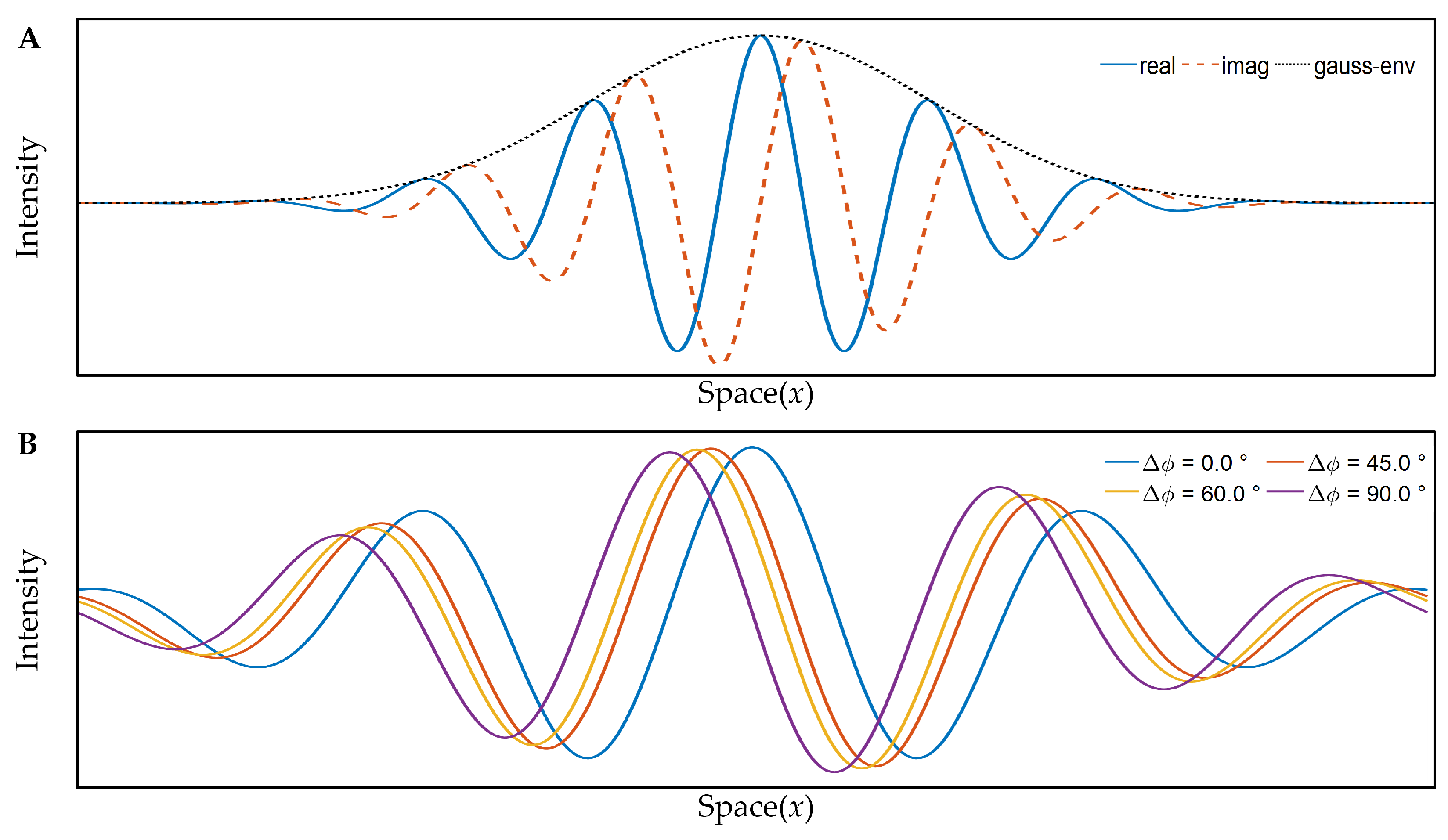
The Complex Morlet Wavelet Transform (CMWT) is a complex-valued, over-complete linear transform for 1D signals. It decomposes a signal into coefficients $W(\sigma ,b,t)$ corresponding to basis functions localized in position b and spatial scale $\sigma$. These basis functions are self-similar, generated through translations and dilations of a mother wavelet ${\psi }_{\sigma }(x-b)$ [22]. Specifically, the analytic Complex Morlet Wavelet mother function is defined in the time domain as a complex sinusoid modulated by a Gaussian envelope (see Figure 1A):

$${\psi }_{\sigma }\left(x\right)={\displaystyle \frac{1}{\sqrt{\sigma }}}·exp\left(-{\displaystyle \frac{x^2}{2{\sigma }^2}}\right)·exp\left(i2\pi f_{c}x\right)$$

(6)

where

$\sigma$ is the scale parameter that controls the spatial width of the wavelet (inversely related to frequency). A larger $\sigma$ corresponds to a broader wavelet and a lower frequency.

$f_c$ is the central frequency of the mother wavelet. For practical purposes, we set $f_c=6$, which ensures that the wavelet is analytic (i.e., its Fourier transform is negligible for negative frequencies when $f_c\ge 5$).

This wavelet is designed to separate the real (even, cosine-based) and imaginary (odd, sine-based) components:

$$\begin{array}{cc}\hfill & \Re \left[{\psi }_{\sigma }\left(x\right)\right]\propto cos(2\pi f_{c}x/\sigma )·e^{-x^2/\left(2{\sigma }^2\right)}\hfill \\ \hfill & \Im \left[{\psi }_{\sigma }\left(x\right)\right]\propto sin(2\pi f_{c}x/\sigma )·e^{-x^2/\left(2{\sigma }^2\right)}\hfill \end{array}$$

(7)

As illustrated in Figure 1B, a spatial translation of the mother wavelet basis corresponds directly to a linear progression in the local phase $\varphi (\sigma ,b,t)$, which establishes the fundamental mathematical link between phase variation and sub-pixel mechanical displacement.

The Gaussian window ensures spatial localization, while the complex sinusoid provides frequency localization within that window. The Continuous Wavelet Transform (CWT) of a 1D signal $f\left(x\right)$ at scale $\sigma$ and position b, using the Complex Morlet Wavelet, is given by the inner product (convolution):

$$W(\sigma ,b,t)=f(x,t)\ast {\psi }_{\sigma }^{*}{\left(x\right)|}_{x=b}={\displaystyle \frac{1}{\sqrt{\sigma }}}{\int }_{-\infty }^{\infty }f(x,t){\psi }_{\sigma }^{*}\left({\displaystyle \frac{x-b}{\sigma }}\right)dx$$

(8)

where ${\psi }_{\sigma }^{*}\left(x\right)$ denotes the complex conjugate of the mother wavelet ${\psi }_{\sigma }\left(x\right)$. The coefficient $W(\sigma ,b,t)$ encodes the local amplitude $A(\sigma ,b,t)$ and the local phase $\varphi (\sigma ,b,t)$ at position b and scale $\sigma$:

$$\begin{array}{cc}\hfill & A(\sigma ,b,t)=\left|W\right(\sigma ,b,t\left)\right|\hfill \\ \hfill & \varphi (\sigma ,b,t)=arg\left(W(\sigma ,b,t)\right)\hfill \end{array}$$

(9)

The local amplitude $A(\sigma ,b,t)$ represents the concentration of energy of the signal component near b that oscillates near the frequency $f_c/\sigma$. The local phase $\varphi (\sigma ,b,t)$ captures the instantaneous phase offset of this oscillatory component, which is directly related to the local structure and position within the Gaussian window.

3.2. Complex Morlet Wavelet Phase-Based Video Magnification (CMW-PVM)

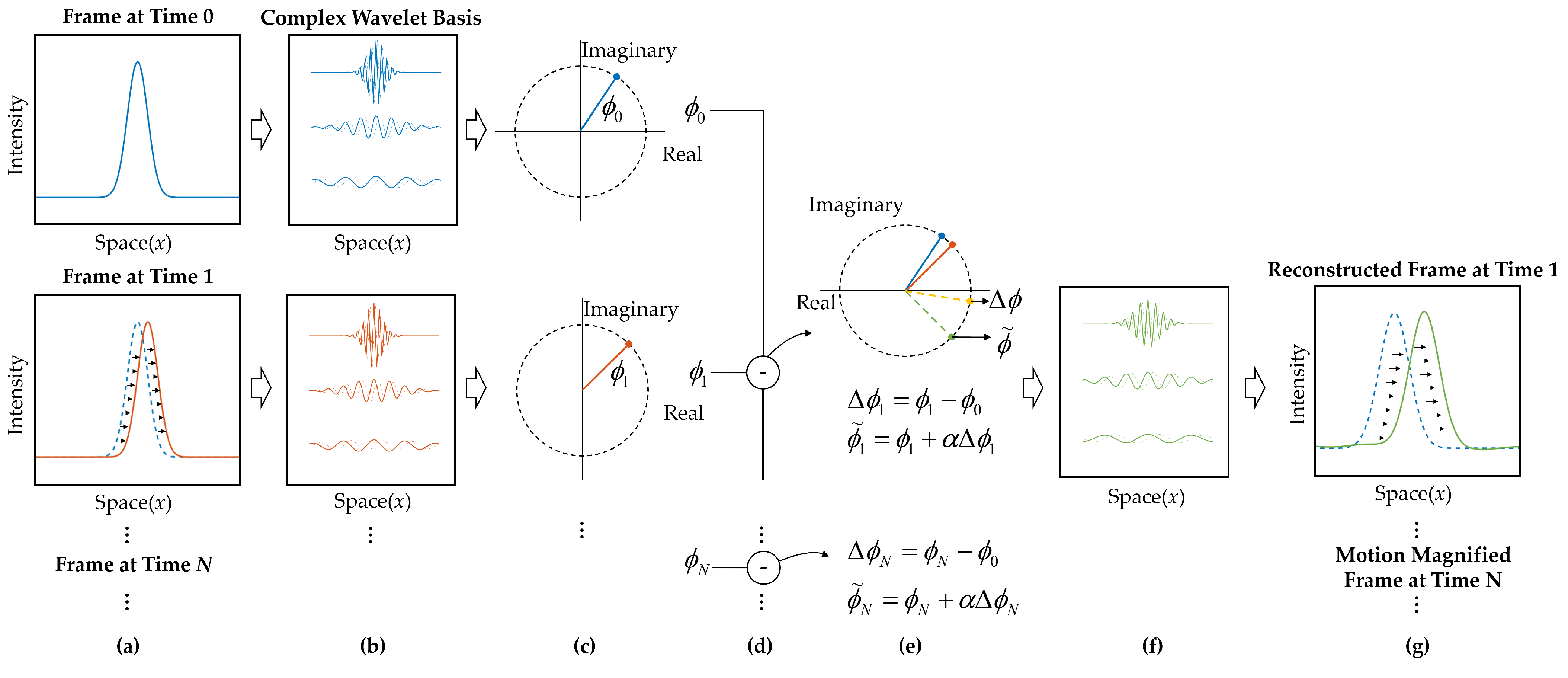
The core of our Phase-Based Video Magnification approach (CMW-PVM) is the amplification of local motion through phase. The amplification is achieved by adjusting the phase of the complex wavelet coefficients while maintaining the amplitude. We now formalize the CMW-PVM approach for the specific case of 1D translational motion of a diffuse object under constant illumination. Figure 2 illustrates the proposed CMW-PVM architecture, with the main steps outlined as follows:

• Wavelet decomposition: For each time t, compute the CWT of each line $I(x,t)$ using the Complex Morlet Wavelet ${\psi }_{\sigma }\left(x\right)$ on relevant scales $\sigma$:

  $$W(\sigma ,b,t)=I(x,t)\ast {\psi }_{\sigma }^{*}{\left(x\right)|}_{x=b}$$

  (10)
• Continuous phase extraction: Extract the local phase map $\varphi (\sigma ,b,t)$ from the complex coefficients:

  $$\varphi (\sigma ,b,t)=arg\left(W(\sigma ,b,t)\right)$$

  (11)
• Temporal phase difference: Compute the localized phase difference relative to a reference frame (e.g., $t_0=0$):

  $$\Delta \varphi (\sigma ,b,t)=\varphi (\sigma ,b,t)-\varphi (\sigma ,b,t_0)$$

  (12)

• Phase amplification: Amplify the phase difference by the factor $\alpha$:

  $$\Delta \tilde{\varphi }(\sigma ,b,t)=\alpha ·\Delta \varphi (\sigma ,b,t)$$

  (13)
• Phase factor reconstruction: Construct a modified complex coefficient that incorporates the amplified phase shift while preserving the original local amplitude:

  $$\begin{array}{cc}\hfill \tilde{W}(\sigma ,b,t)& =W(\sigma ,b,t)·e^{i\alpha \Delta \varphi (\sigma ,b,t)}\hfill \\ \hfill & =\left|W(\sigma ,b,t)\right|·e^{i\left(\varphi \right(\sigma ,b,t)+\alpha \Delta \varphi (\sigma ,b,t\left)\right)}\hfill \end{array}$$

  (14)
  This step effectively rotates the coefficient in the complex plane. Theoretically, for an analytic wavelet, a local spatial translation $\delta \left(t\right)$ manifests as a linear phase shift $\Delta \varphi \approx \xi ·\delta \left(t\right)$. By augmenting the instantaneous phase to $\varphi +\alpha \Delta \varphi \approx {\varphi }_0+(1+\alpha )\xi \delta \left(t\right)$, the subsequent inverse transform maps this total phase shift back into the spatial domain, directly yielding the magnified profile $\tilde{I}(x,t)=f(x+(1+\alpha )\delta \left(t\right))$.
• Inverse Wavelet Transform: Reconstruct the magnified spatial signal $\widehat{I}(x,t)$ at each time t using the Inverse Continuous Wavelet Transform (ICWT). For an overcomplete transform like the CMWT, this is achieved by summation over scales and positions using the real-valued synthesis wavelet or directly via

  $$\widehat{I}(x,t)=\Re \left[\sum _{\sigma }{\displaystyle \frac{1}{C_{\psi }}}{\displaystyle \frac{1}{{\sigma }^p}}{\int }_{-\infty }^{\infty }\tilde{W}(\sigma ,b,t){\psi }_{\sigma }(x-b)db\right]$$

  (15)

  where $C_{\psi }$ is a constant depending on the wavelet, p is an exponent related to the reconstruction norm (often $p=2$), and $\Re [·]$ extracts the real part. In practice, discrete approximations and specific reconstruction filters are used to ensure numerical stability and reproducibility.

To ensure the reproducibility of the proposed CMW-PVM method (as shown in Algorithm 1), the specific implementation choices and computational environment are detailed as follows. The temporal band-pass filtering stage utilizes a 4th-order Butterworth filter to isolate the target motion frequency $f_m$. The cut-off frequencies are adaptively set as $[f_L,f_H]=[f_m-20,f_m+20]$ Hz, providing a 40 Hz pass-band centered at the fundamental oscillation to suppress out-of-band sensor noise. For signal reconstruction, the Inverse Continuous Wavelet Transform (ICWT) incorporates the admissibility constant $C_{\psi }$ specific to the Complex Morlet kernel to ensure energy conservation during the phase-to-intensity mapping.

Algorithm 1 CMW-PVM pipeline implementation details
Require: 1D line-scan sequence $I(x,t)$, magnification factor $\alpha$, wavelet scale $\sigma$, central frequency $f_c=6$, band-pass frequency range $[f_L,f_H]$
Ensure: Magnified spatiotemporal signal $\widehat{I}(x,t)$
// Step 1: Preprocessing
for each time step $t\in [0,T]$ do
$I(x,t)\leftarrow \mathrm{Normalize}\left(I\right(x,t\left)\right)$	▹ Normalize intensity to $[0,1]$
$I_{pad}(x,t)\leftarrow \mathrm{Padding}\left(I(x,t)\right)$	▹ Zero-padding for FFT efficiency
end for
// Step 2: Complex Morlet Wavelet Decomposition
for each time step t do
$W(\sigma ,b,t)\leftarrow \mathrm{CWT}(I_{pad}(x,t),{\psi }_{\sigma })$	▹ Using Equation (14)
$A(\sigma ,b,t)\leftarrow \left|W\right(\sigma ,b,t\left)\right|$	▹ Extract local amplitude
$\varphi (\sigma ,b,t)\leftarrow \arg \left(W\right(\sigma ,b,t\left)\right)$	▹ Extract local phase
end for
// Step 3: Phase Manipulation and Noise Decoupling
$\Delta \varphi (\sigma ,b,t)\leftarrow \varphi (\sigma ,b,t)-\varphi (\sigma ,b,0)$	▹ Compute phase difference
$\Delta {\varphi }_{filt}(\sigma ,b,t)\leftarrow \mathrm{BandPassFilter}(\Delta \varphi ,[f_L,f_H])$	▹ Butterworth or Ideal filter
$\Delta \tilde{\varphi }(\sigma ,b,t)\leftarrow \alpha ·\Delta {\varphi }_{filt}(\sigma ,b,t)$	▹ Apply magnification factor
// Step 4: Reconstruction
for each time step t do
$\tilde{W}(\sigma ,b,t)\leftarrow A(\sigma ,b,t)·e^{i(\varphi (\sigma ,b,t)+\Delta \tilde{\varphi }(\sigma ,b,t))}$	▹ Modify phase only
$\widehat{I}(x,t)\leftarrow \mathrm{Re}\left\{\mathrm{ICWT}\left(\tilde{W}(\sigma ,b,t)\right)\right\}$	▹ Inverse CWT reconstruction
end for
return $\widehat{I}(x,t)$

4. Simulation Evaluation and Discussion

To assess the efficacy of the proposed Complex Morlet Wavelet phase video magnification (CMW-PVM) method, we theoretically examined the limitations of critical parameters to provide empirical guidance, subsequently developing simulations for comparison with traditional Eulerian video magnifier (EVM) and phase video magnifier (PVM) methods.

4.1. Parameters and Boundary Conditions

All motion magnification approaches possess fundamental boundary conditions beyond which amplification generates severe artifacts. For Eulerian Video Magnification (EVM) [11], the underlying first-order Taylor approximation fails when spatial displacements $\delta \left(t\right)$ are large. Consequently, its amplification factor $\alpha$ is strictly bounded by the dominant spatial wavelength $\lambda$:

$$(1+\alpha )\delta \left(t\right)\le {\displaystyle \frac{\lambda }{8}}$$

(16)

Furthermore, EVM linearly amplifies intensity noise, severely limiting its practical magnification scale.

Similarly, Phase-Based Video Magnification (PVM) [19] is governed by the phase wrapping limit to prevent aliasing artifacts (i.e., $\alpha \Delta \varphi \le \pi$). Given the phase-displacement relationship $\Delta \varphi =2\pi \delta \left(t\right)/\lambda$, its physical constraint translates to $\alpha \delta \left(t\right)\le \lambda /4\pi$. Both EVM and PVM reveal a critical vulnerability: higher spatial frequencies (smaller $\lambda$) impose stricter magnification ceilings. Additionally, PVM’s reliance on global Fourier spatial homogeneity often causes phase distortions and linear noise amplification when processing localized complex motions.

To mitigate these global constraints, the proposed CMW-PVM establishes mathematically localized boundaries for its core parameters.

4.1.1. Limitation for Gain Coefficient $\alpha$

The gain coefficient $\alpha$ dictates the degree of amplification of motion. In CMW-PVM, excessive $\alpha$ will induce non-physical phase wrapping beyond the principal range $(-\pi ,\pi ]$. Based on the local phase approximation $\Delta \varphi (\sigma ,b,t)\approx {\xi }_{\sigma }\left(b\right)·\delta \left(t\right)$ derived in Section 3.2, the necessary condition to prevent phase wrapping is

$$|\alpha ·\Delta \varphi (\sigma ,b,t\left)\right|\le \pi ,\forall b,t$$

(17)

Substituting the local approximation yields the precise theoretical upper bound for $\alpha$:

$$\alpha \le {\displaystyle \frac{\pi }{{\xi }_{max}·{\delta }_{max}}}$$

(18)

Here, ${\xi }_{max}$ (radians/pixel) denotes the maximum spatial frequency at which the wavelet exhibits the highest sensitivity to local structural changes, while ${\delta }_{max}$ (pixels) is the maximum expected displacement. Unlike global methods, this formulation indicates that the applicable gain limit is adaptively determined by highly localized spatial textures and regional displacements.

A comprehensive comparison of theoretical constraints and noise sensitivities is summarized in

Table 1. Comparison of constraints and applicability among different video motion magnification methods.

Method	Magnification Constraint ($\mathit{\alpha }$)	Applicable Scenarios	Noise Sensitivity
EVM [11]	$(1+\alpha )\delta \le {\displaystyle \frac{\lambda }{8}}$	Global translation, low texture complexity	High (Linear amplification)
PVM [19]	$\alpha \delta \le {\displaystyle \frac{\lambda }{4\pi }}$	Global translation, medium texture	High (Phase noise)
CMW-PVM	$\alpha \le {\displaystyle \frac{\pi }{{\xi }_{max}{\delta }_{max}}}$	Local complex motion, multi-scale structures	Low (Local phase retention)

. Although EVM and PVM exhibit theoretical gain bounds dependent on global wavelengths, their practical effectiveness is severely capped by early noise-driven saturation. In contrast, CMW-PVM inherently incorporates spatial localization (${\xi }_{max}$) and limits phase noise propagation. This results in an amplification factor that scales robustly within a predictable and physically interpretable saturation limit, significantly outperforming conventional global methods.

4.1.2. Time–Frequency Locality Constraint for the Wavelet Scale $\sigma$

The wavelet scale $\sigma$ governs the fundamental trade-off between spatial localization and frequency resolution in the CMW-PVM method. An optimal $\sigma$ must capture the target motion while simultaneously suppressing high-frequency noise and avoiding spatial blurring. This establishes a definitive operational interval.

• 1. Lower Bound Constraint: Spectral Matching and Noise Suppression

The lower bound for $\sigma$ ensures that the wavelet avoids excessive sensitivity to high-frequency noise. Specifically, the effective carrier frequency of the wavelet $f_{\sigma }=f_c/\sigma$ must not exceed the characteristic spatial frequency of the target movement $f_{\mathrm{motion}}=1/{\lambda }_{\mathrm{motion}}$. This prevents the wavelet from predominantly responding to high-frequency interference:

$$f_{\sigma }\le f_{\mathrm{motion}}\Rightarrow {\displaystyle \frac{f_c}{\sigma }}\le {\displaystyle \frac{1}{{\lambda }_{\mathrm{motion}}}}\Rightarrow \sigma \ge f_c·{\lambda }_{\mathrm{motion}}$$

(19)

According to Equation (6), the central frequency $f_c$ is typically set to 6. Therefore, the lower bound is strictly dictated by the frequency matching condition:

$${\sigma }_{min}=6{\lambda }_{\mathrm{motion}}$$

(20)

• 2. Upper Bound Constraint: Validity of Local Motion Assumption

The CMW-PVM method estimates motion based on the locally stationary motion hypothesis, assuming the displacement field is approximately uniform within the wavelet’s spatial support region. If $\sigma$ is excessively large, its spatial window ${\mathcal{W}}_{\sigma }$ will encompass areas with diverse motion patterns, leading to blurred motion and phase distortion.

To maintain local validity, the effective spatial support width of the wavelet (${\mathcal{W}}_{\mathrm{spatial}}\approx 2.35\sigma$) must not exceed the scale at which the motion experiences significant variation ($L_{\mathrm{motion}-\mathrm{variation}}$):

$${\mathcal{W}}_{\mathrm{spatial}}\le L_{\mathrm{motion}-\mathrm{variation}}\Rightarrow 2.35\sigma \le L_{\mathrm{motion}-\mathrm{variation}}$$

(21)

This yields a concise spatial locality constraint:

$${\sigma }_{max}={\displaystyle \frac{L_{\mathrm{motion}-\mathrm{variation}}}{2.35}}\approx 0.426L_{\mathrm{motion}-\mathrm{variation}}$$

(22)

In general, the complete theoretical constraint interval for the scale parameter $\sigma$ is defined by two intrinsic spatial scales of the target motion.

$$6{\lambda }_{\mathrm{motion}}\le \sigma \le 0.426L_{\mathrm{motion}-\mathrm{variation}}$$

(23)

This dual-scale boundary elegantly balances time–frequency resolution. It provides explicit theoretical guidance for practical parameter selection: the lower bound ensures spectral matching to suppress noise, while the upper bound preserves spatial locality to maintain the linearity of the phase-motion relationship.

4.2. Simulation Framework and Performance Evaluation Metrics

To ensure a rigorous and fair benchmark, we selected the 1D implementations of EVM and PVM as baselines. It is important to note that although these methods are widely known for 2D area-scan applications, their mathematical foundations—namely, the first-order Taylor expansion for EVM and the Fourier shift theorem for PVM—are fundamentally derived from 1D signal analysis. Therefore, the 1D-based versions of these algorithms are the most appropriate for this specific line-scan architecture. In contrast, modern learning-based methods [13] are inherently designed for 2D spatial feature extraction, making them unsuitable for our 1D spatiotemporal signal stream.

Based on the theoretical constraint analysis of EVM, PVM, and CMW-PVM, the derived boundaries for amplification coefficients and phase continuity provide essential guidance for experimental design. To quantitatively assess the proposed method, we constructed a controlled 1D simulation model. This framework generates the ground truth at the pixel-level, enabling the precise quantification of magnification performance, robustness, and operational limits.

4.2.1. Signal Generation and Motion Modeling

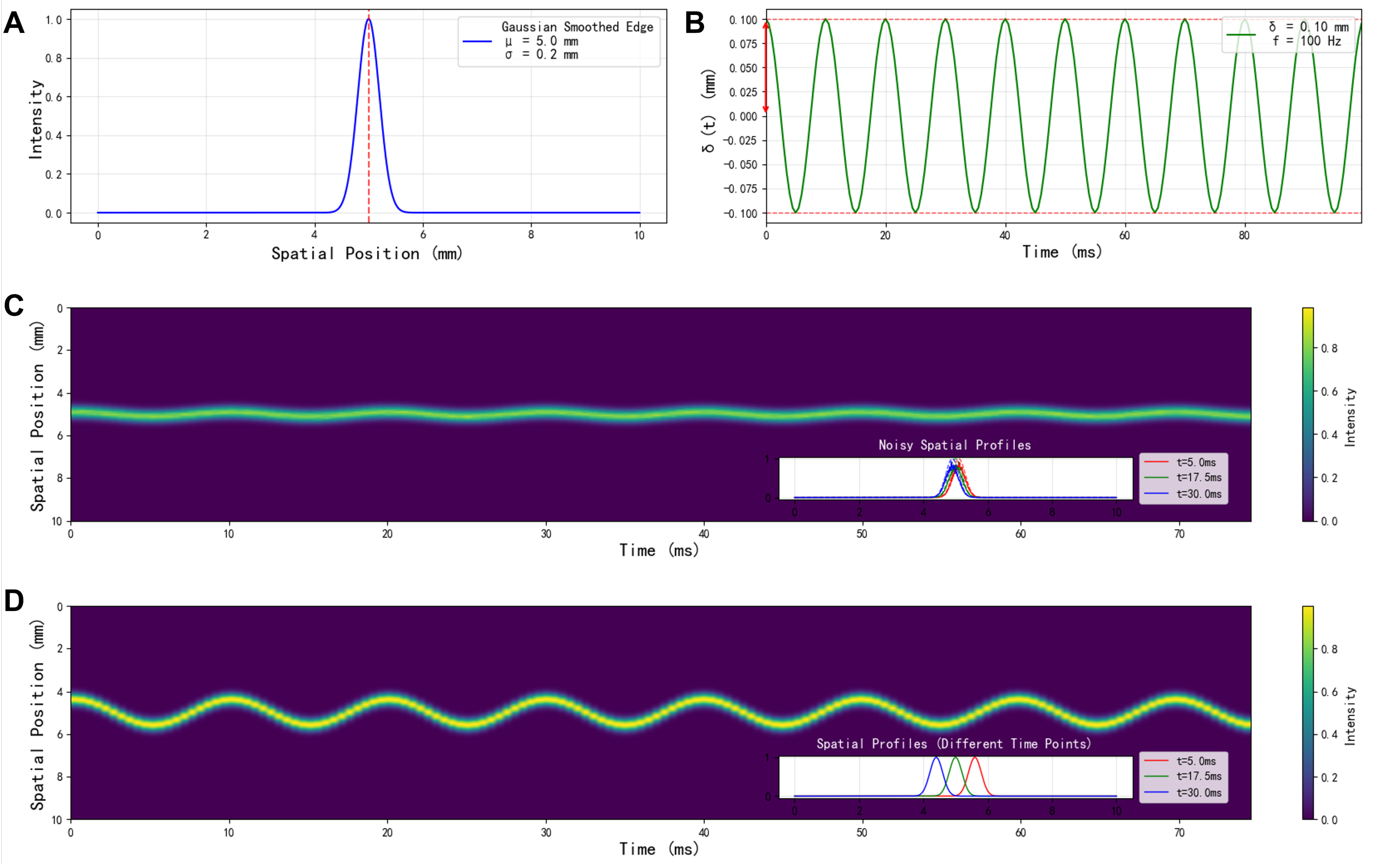
The simulation utilized a Gaussian intensity profile $I\left(x\right)=exp(-{(x-\mu )}^2/2{\sigma }^2)$ to represent a smooth edge, providing a continuous gradient for sub-pixel estimation.

To simulate sub-pixel displacements $\delta \left(t\right)$ with high kinematic fidelity, we employed a high-order cubic spline interpolation scheme. Specifically, for each time step t, a continuous cubic spline function $S\left(x\right)$ was constructed from the discrete reference signal. This function ensured second-order derivative continuity ($C^2$), which is critical for preventing artificial phase jumps during wavelet decomposition. The shifted signal was then generated by re-sampling the spline at the translated coordinates $x-\delta \left(t\right)$. Compared to linear interpolation, this high-order approach minimizes intensity quantization errors and ensures that the simulated motion is perceived as a smooth, physically-consistent translation rather than a numerical artifact. The simulation and experimental processing pipelines were developed using Python 3.9.0. Key libraries include NumPy (v2.0.2) for high-performance complex-valued matrix operations and OpenCV-Python (v4.13.0.92) for spatiotemporal data handling. In the simulation benchmark (Section 4), the magnification factor $\alpha$ was swept from 1 to 50 with a step of 1, and the input noise levels were varied between SNR = 10 dB and 30 dB to rigorously evaluate gain linearity and robustness boundaries.

To simulate real-world sensor limitations, the raw sequence was corrupted with additive white Gaussian noise. The resulting spatiotemporal map (Figure 3C) exhibits characteristic intensity fluctuations used to test the robustness of phase-based extraction. To evaluate magnification accuracy, a ground-truth signal $I_{GT}(x,t)$ was defined by applying the target amplified displacement ${\delta }_{GT}\left(t\right)=(1+\alpha )\delta \left(t\right)$ to the original profile (Figure 3D).

This model provides a reference with precisely known values and a clear geometric meaning. To ensure statistical significance, we sweep multiple noise levels (e.g., varying input SNR) and report averaged results across multiple random seeds. For a fair comparison, all methods (EVM, PVM, and CMW-PVM) operate on the same noisy input and utilize the same temporal band-pass filter centered at $f_m$. This ensures that performance variances arise solely from the spatial representation—specifically, the distinction between Eulerian intensity, global Fourier phase, and local wavelet phase.

4.2.2. Performance Evaluation Metrics

To comprehensively evaluate the algorithms, we employed two complementary families of metrics: motion magnification accuracy and video fidelity. These metrics quantify the precision of the motion extraction and the linearity of the amplification:

• 1. Displacement Root Mean Square Error (RMSE)

RMSE measures the root mean square error between the estimated amplified displacement $\delta \left(t\right)$ and the ground truth ${\delta }_{GT}\left(t\right)$.

$$RMS{E}_{\delta }=\sqrt{{\displaystyle \frac{1}{T}}\sum _t{(\widehat{\delta }\left(t\right)-{\delta }_{GT})}^2}$$

(24)

• 2. Harmonic Distortion Index (HDI)

The HDI is the ratio of energy in the higher harmonics to the fundamental frequency $f_m$. This reflects spurious artifacts introduced when phase-continuity or linearity assumptions fail.

• 3. Peak Signal-to-Noise Ratio (PSNR)

The PSNR evaluates reconstruction fidelity by calculating the ratio between the maximum possible power of the signal and the Mean Squared Error (MSE) between the amplified result and the ground truth $I_{GT}$:

$$PSNR=10·lo{g}_{10}\left({\displaystyle \frac{L^2}{MSE}}\right)$$

(25)

where L is the dynamic range of the pixel values. A higher PSNR indicates superior pixel-level precision and reduced distortion.

• 4. Feature Similarity Index Measure (FSIM)

In the context of motion magnification, excessive amplification often induces structural distortion or edge blurring (ringing artifacts). Standard metrics like the Peak Signal-to-Noise Ratio (PSNR) evaluate global pixel-wise errors but fail to align with the human visual system’s perception of structural fidelity. To rigorously quantify the structural preservation capacity of the proposed CMW-PVM algorithm, the Feature Similarity Index Measure (FSIM) was adopted as the primary evaluation metric.

The FSIM is explicitly designed to assess image quality based on two low-level features that are crucial for structural perception: phase congruence (PC) and gradient magnitude (GM) [23]. The evaluation compares the reference (unmagnified or ground truth) $im{g}_1$ and the distorted (magnified) image $im{g}_2$. Its mathematical model is as follows:

$$\begin{array}{c}FSIM={\displaystyle \frac{{\sum }_{x\in \Omega }{S}_{L}P{C}_{max}\left(x\right)}{{\sum }_{x\in \Omega }P{C}_{max}\left(x\right)}}\\ S_L\left(x\right)={\left[S_{PC}\left(x\right)\right]}^a{\left[S_G\left(x\right)\right]}^b\\ S_{PC}\left(x\right)={\displaystyle \frac{2P{C}_1\left(x\right)P{C}_2\left(x\right)+T_1}{P{C}_1^2\left(x\right)+P{C}_2^2\left(x\right)+T_1}}\\ S_G\left(x\right)={\displaystyle \frac{2G_1\left(x\right)G_2\left(x\right)+T_2}{G_1^2\left(x\right)+G_2^2\left(x\right)+T_2}}\end{array}$$

(26)

where $P{C}_1$ and $P{C}_2$ denote the phase congruency of $im{g}_1$ and $im{g}_2$, respectively, and $P{C}_{\max }=max(P{C}_1,P{C}_2)$. The gradient magnitudes of $im{g}_1$ and $im{g}_2$ are represented by $G_1$ and $G_2$, respectively. $T_1$ and $T_2$ are positive constants, and a and b are two constants.

4.3. Performance Benchmark and Comparative Analysis

Drawing on aforementioned theoretical constraints and the experimental design, this section aims to evaluate and compare the performance of three methods: the linear Eulerian video magnifier (EVM), the phase-based video magnifier (PVM), and the proposed Complex Morlet Wavelet-based phase video magnifier (CMW-PVM). Using the quantitative metrics defined in Section 4.2, the analysis focuses on the accuracy of the amplification, noise robustness, and distortion characteristics of each method under various simulation conditions. These evaluations serve to validate the superiority and applicable scope of the CMW-PVM approach.

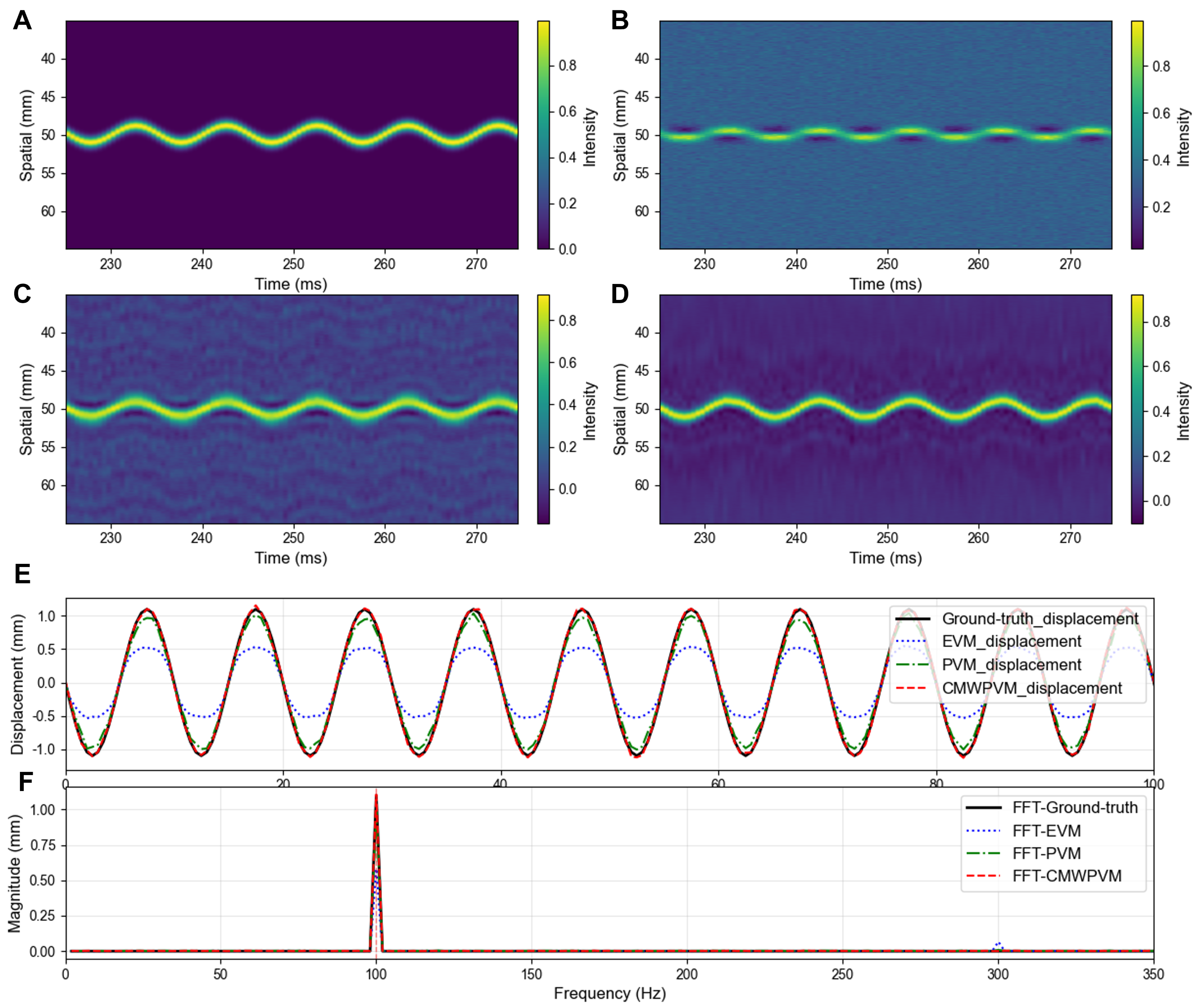
The spatiotemporal diagrams (Figure 4A–D) illustrate the motion reconstruction capabilities of each method. Figure 4A represents the amplified signal of the ground truth. The EVM result (Figure 4B) exhibits severe signal attenuation and discontinuity, a known limitation when the product of the amplification factor and displacement exceeds the spatial wavelength. PVM (Figure 4C) successfully recovers the oscillation pattern but suffers from significant phase noise and background artifacts. In contrast, the CMW-PVM output (Figure 4D) shows the highest correspondence to the ground truth, maintaining a high contrast-to-noise ratio and a smooth reconstruction of the wavefront.

The time-domain displacement analysis (Figure 4E) further quantifies these observations. The EVM significantly underestimates the displacement amplitude due to its restricted linear approximation range. Although PVM tracks periodic motion more effectively, it introduces visible fluctuations at the oscillation peaks. Conversely, CMW-PVM yields a trajectory nearly indistinguishable from the ground truth. This precision is attributed to the localized multi-resolution properties of the Complex Morlet Wavelet, which ensures robust phase estimation under noisy conditions.

To assess spectral fidelity, the fast Fourier transform (FFT) spectra of the estimated displacements are compared (Figure 4F). Although all methods identify the primary 100 Hz frequency, EVM exhibits a distinct secondary peak at the third harmonic (300 Hz). This harmonic leakage and waveform clipping indicate severe non-linear distortion, confirming that the motion has exceeded the Taylor series expansion constraints. Similarly, the overall magnitude reduction in both EVM and PVM indicates a breakdown of algorithmic saturation at $\alpha =10$. In contrast, CMW-PVM yields a clean, high-magnitude peak at 100 Hz with negligible harmonics, successfully avoiding the non-linear artifacts that plague conventional methods.

These simulation results validate the theoretical boundaries established in Section 4.1. Under typical operational conditions, CMW-PVM exhibits superior linearity, spectral fidelity, and noise suppression. To comprehensively delineate these advantages, parametric experiments were conducted across a broader spectrum of noise levels and magnification factors, utilizing quantitative image- and displacement-domain metrics.

4.4. Comprehensive Analysis of Algorithm Performance Boundaries and Robustness

This section comprehensively evaluates the performance boundaries of the algorithms across three critical dimensions: gain linearity, visual fidelity, and noise robustness.

4.4.1. Dynamic Magnification Range and Gain Linearity

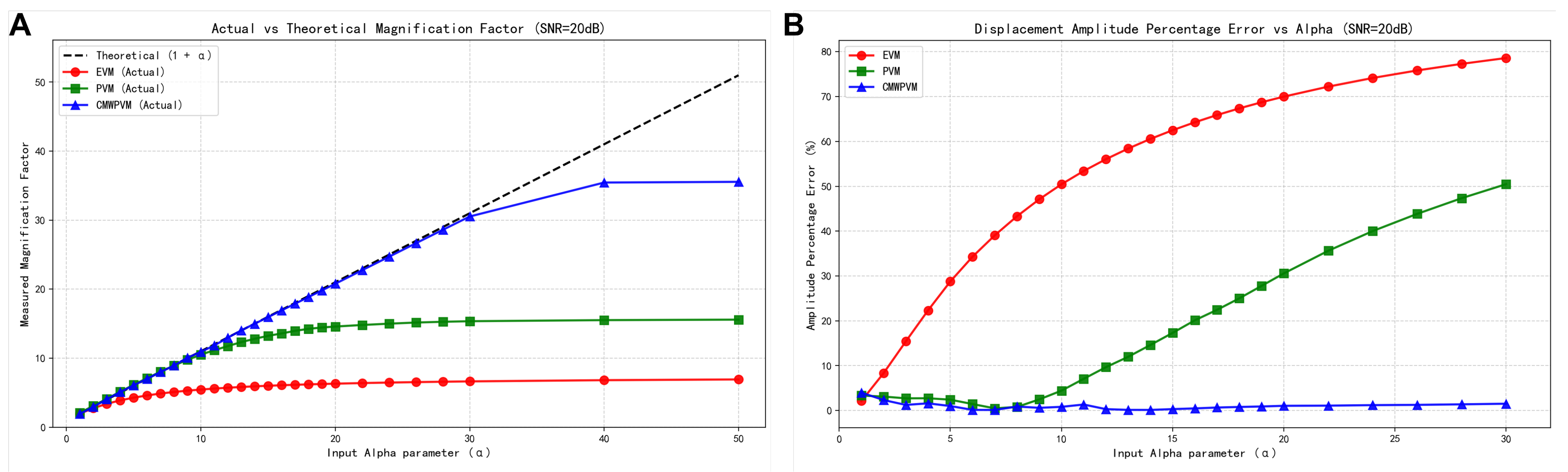
In motion magnification tasks, the effective dynamic range is fundamentally determined by the algorithm’s capacity to preserve gain linearity—the fidelity with which the actual output magnification approximates the theoretical magnification factor $(1+\alpha )$. To evaluate this, we systematically investigated the saturation boundaries and amplitude errors of the three algorithms with a standardized noise floor (SNR = 20 dB).

As illustrated in Figure 5A, EVM deviates from the theoretical baseline at a very early stage ($\alpha \approx 5$), corroborating its well-known sensitivity to noise and truncation errors with the Taylor first-order approximation. By shifting to the phase domain, PVM successfully extends the operational range. However, it plateaus near $\alpha \approx 15$. This indicates that under noisy conditions, the large, localized phase shifts induced by high magnification factors easily trigger global phase wrapping, causing the global Fourier transform to yield unstable or noisy phase estimations.

In contrast, CMW-PVM closely tracks the theoretical baseline in a significantly broader operational window, with saturation only emerging beyond $\alpha \approx 35$. The spatiotemporal localization characteristic of the Complex Morlet Wavelet effectively isolates noise and prevents the global phase distortions that cripple PVM.

The corresponding amplitude error dynamics (Figure 5B) further expose the underlying stability differences. As summarized in

Table 2. Comprehensive comparison of dynamic performance among three motion magnification algorithms at SNR = 20 dB.

Method	Saturation Knee Point ($\mathit{\alpha }$)	Max Actual Magnification	Amplitude Error at $\mathit{\alpha }=15$	Amplitude Error at $\mathit{\alpha }=30$
EVM	≈5	≈7	>40%	≈80%
PVM	≈15	≈15	≈20%	≈50%
CMW-PVM	≈35	≈36	<3%	<3%

, CMW-PVM maintains kinematic fidelity within an order of magnitude superior to traditional methods with high magnification regimes. While traditional Eulerian and global phase-based techniques are fundamentally constrained by early saturation and severe amplitude degradation, CMW-PVM keeps the amplitude percentage error strictly suppressed below 3% throughout the tested range, establishing its reliability for large-scale micro-motion extraction.

4.4.2. Fidelity Degradation and Motion Accuracy Analysis

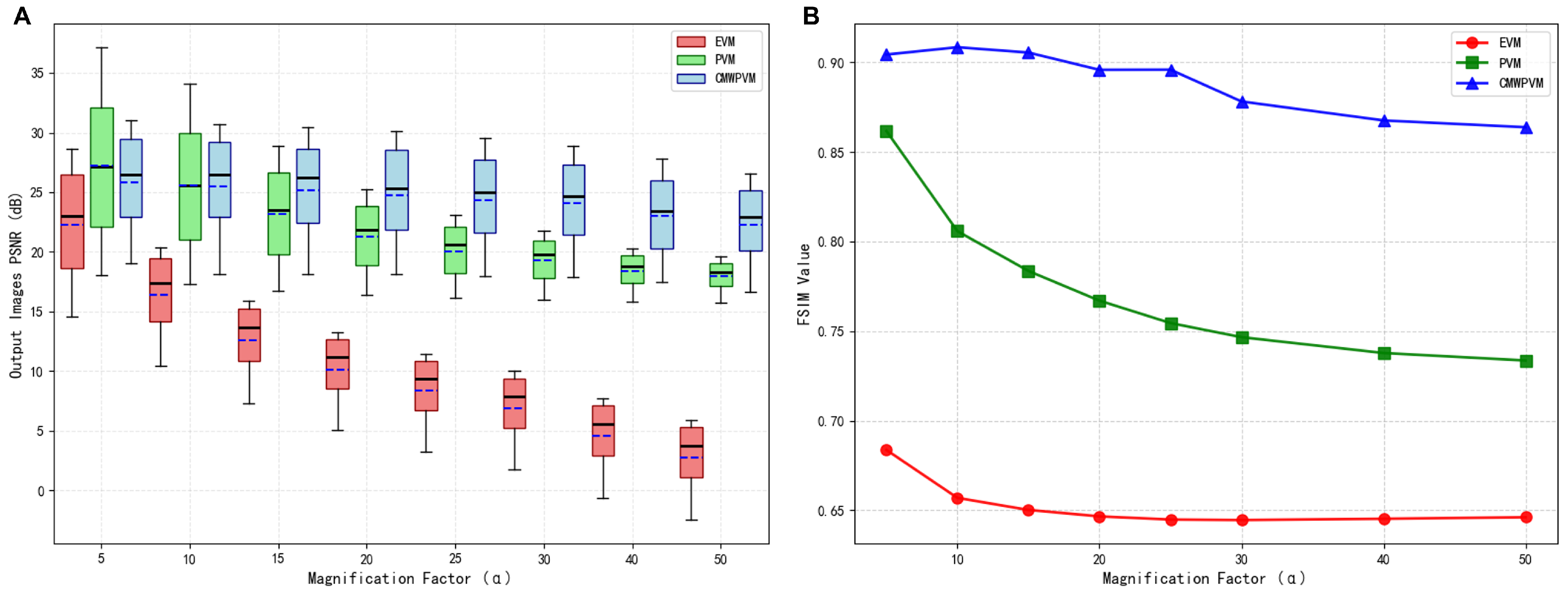
Although increasing $\alpha$ is mathematically feasible, it inevitably introduces background noise and structural artifacts. This section quantitatively compares visual fidelity and kinematic accuracy with extreme magnification regimes ($\mathrm{SNR}=20\mathrm{dB}$).

Figure 6A,B illustrate the degradation trends of the PSNR and FSIM for $\alpha \in [5,50]$. As expected, EVM suffers the most severe degradation, with the lowest overall PSNR values and FSIM scores stagnating at an unacceptable baseline due to linear noise amplification.

PVM provides a noticeable improvement in the low $\alpha$ range but deteriorates significantly as the magnification intensifies. Its FSIM curve drops sharply beyond $\alpha =10$. This structural collapse is driven by the violation of global phase continuity: heavily amplified localized motions cause phase wrapping in the global Fourier basis, physically manifesting as spatial ringing artifacts. In contrast, CMW-PVM strictly confines phase manipulation within localized spatiotemporal wavelet supports, effectively preventing noise propagation. Consequently, its FSIM remains stable within a high-quality threshold (0.87–0.91) even at $\alpha =50$, along with the most compact PSNR interquartile ranges.

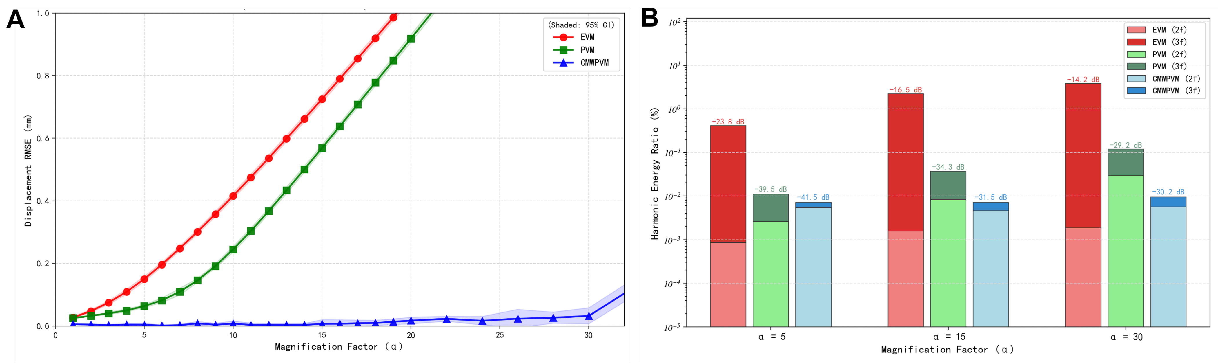
The precision of kinetic measurement (Figure 7A) reveals a distinct performance hierarchy. The rapid divergence of EVM’s RMSE confirms the breakdown of its linear approximation model. PVM exhibits a linear RMSE growth trajectory, indicating that global phase processing accumulates errors when handling large-scale motions. Conversely, CMW-PVM maintains a near-zero RMSE baseline (<0.1 mm) with extremely narrow 95% confidence intervals, demonstrating highly reproducible displacement estimates.

Spectral analysis of these errors (Figure 7B) shows that both EVM and PVM exhibit significant harmonic leakage as $\alpha$ increases (e.g., surge energy $3f$ for EVM and increase total harmonic energy for PVM). In contrast, the harmonic energy of CMW-PVM remains negligible (below $-30$ dB). By avoiding global phase discontinuities, CMW-PVM confines the motion signal within the linear phase regime, ensuring that the amplified output is free from spurious frequency artifacts.

4.4.3. Noise Evolution Mechanisms and Robustness Analysis

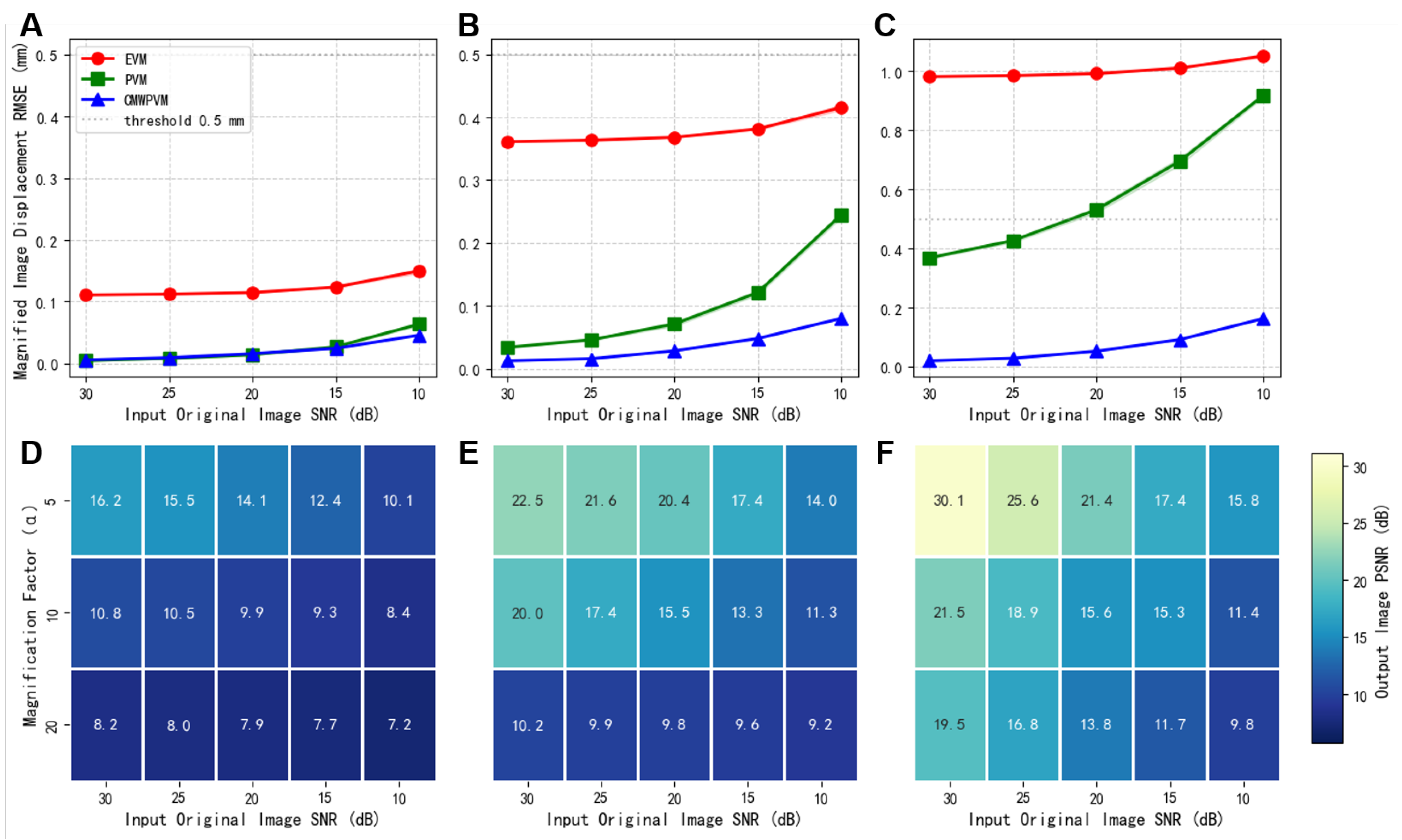
In practical engineering applications, video inputs are inevitably contaminated by variable sensor noise. To evaluate algorithmic robustness, this section simulates continuous input SNRs from 30 dB (clean) to 10 dB (extreme noise) at fixed magnification levels ($\alpha =5,10,20$).

Figure 8A–C illustrate the evolution of displacement RMSE. As input SNR decreases, all methods exhibit an upward trend in error, exacerbated by larger magnification factors. EVM consistently presents the highest baseline error. PVM shows a moderate increase in error at lower magnifications, but its trajectory becomes critically steep at $\alpha =20$ as the SNR drops, indicating that the global Fourier phase is highly fragile and prone to catastrophic unwrapping failures under heavy noise conditions. However, CMW-PVM exhibits a remarkably flat growth rate. Even under the compound stress of $\alpha =20$ and $\mathrm{SNR}=10\mathrm{dB}$, its maximum RMSE is well below 0.2 mm. This suggests that the localized spatiotemporal support of the Complex Morlet Wavelet acts as a dynamic band-pass filter, preventing random noise from corrupting the kinematic trajectory.

The output PSNR heat maps (Figure 8D–F) provide a holistic view of signal preservation. EVM (Figure 8D) is dominated by cool colors with steep degradation gradients. Although PVM (Figure 8E) improves globally by 5 to 7 dB, its vertical degradation at magnification levels remains significant. The CMW-PVM heat map (Figure 8F) is distinguished by extensive warm regions, which achieve up to 30.1 dB under optimal conditions. More importantly, its horizontal and vertical degradation rates are remarkably gentle. By decoupling the motion phase from global noise via localized wavelet analysis, CMW-PVM mitigates the severe noise amplification effects that constrain traditional algorithms.

4.5. Summary of Simulation Results, Methodological Performance, and Limitations

Extensive controlled simulations quantitatively validated the theoretical advantages of the proposed CMW-PVM framework. Compared to traditional EVM and PVM, the proposed method demonstrates a significantly broader dynamic magnification range (maintaining strict linearity up to $\alpha \approx 35$), exceptional structural fidelity (FSIM $>0.87$), sub-pixel kinematic accuracy, and robust noise immunity under severe dual-stress conditions.

The selection of baselines was strategically limited to the 1D analytical kernels of EVM and PVM. Recent 2D phase-based and learning-based techniques were excluded as they primarily prioritize visual magnification tasks, focusing on artifact suppression and perceptual realism. While these 2D methods can produce visually impressive magnified videos, they lack a deterministic and linear relationship between the input magnification factor $\alpha$ and the reconstructed physical displacement. In contrast, our 1D CMW-PVM is designed for quantitative metrology, where the localized phase-to-motion mapping ensures that the magnified output maintains a strict, traceable correspondence to the actual vibration amplitude.

Despite its performance, several limitations of the 1D CMW-PVM must be acknowledged. First, the 1D architecture restricts motion acquisition to a single spatial axis, making it unsuitable for complex scenes requiring full 2D modal analysis or multi-directional non-rigid deformations. Second, concerning the sampling theorem, we clarify that the system resolves high-frequency dynamics not by “violating” Nyquist–Shannon limits but by leveraging the high physical sampling rate (exceeding 10 kHz) of line-scan sensors. This hardware advantage ensures that vibrations remain well within the sensor’s folding frequency, effectively avoiding the aliasing artifacts prevalent in conventional 2D vision systems.

Furthermore, while robust against Gaussian noise, the method’s performance under conditions of extreme illumination fluctuations or non-periodic transient impulses requires further evaluation to ensure industrial generalizability. We deployed the algorithm on actual high-speed line-scan video sequences to verify its metrological accuracy.

5. Experimental Verification and Discussion

5.1. Experimental Setup and Data Acquisition

To comprehensively evaluate the practical performance of the proposed CMW-PVM algorithm, a controlled laboratory experiment was conducted using a precision linear motion platform.

Instead of traditional contact-based sensors, a Polytec OFV-5000 high-performance single-point laser Doppler vibrometer (LDV) (Polytec GmbH, Waldbronn, Germany) was employed as the reference standard for ground-truth measurement. It boasts exceptionally high measurement resolution and a massive dynamic range, ensuring reliability without introducing any mass-loading effects to the moving structure. In this experiment, the motion extraction results processed by our vision-based algorithm were directly compared against the highly accurate reference signals acquired by the LDV.

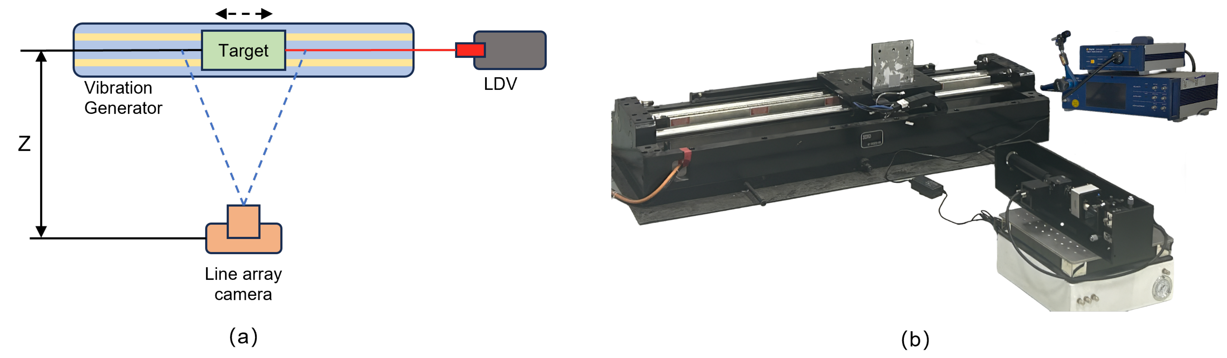
Figure 9 depicts the experimental setup, comprising the schematic representation of the optical arrangement (Figure 9a) and the tangible physical apparatus (Figure 9b). The target plate was firmly attached to a motorized linear stage to produce regulated dynamic displacements. To ensure a thorough comparative analysis, the target’s vibration was concurrently recorded using both the LDV and the proposed vision-based sensor (line-scan camera).

The LDV optical head was strategically positioned to send a laser beam onto the target, thereby capturing its instantaneous displacement. Simultaneously, the line-scan camera, fitted with an industrial optical lens, was securely affixed to an optical vibration-isolation table. The camera was positioned roughly $0.8$ m from the target, with its optical axis oriented to guarantee that the target’s motion edge consistently remained within the 1D imaging sensor line. This dual-sensor non-contact system ensured that both devices saw the identical dynamic event without physical interference.

In the data collection procedure, the Polytec OFV-5000 LDV’s sampling frequency was established at 1000 Hz to obtain high-fidelity reference signals. Similarly, the line-scan camera continuously recorded the spatial profile at a line rate of 1000 Hz, achieving a spatial resolution of 2048 pixels per line. A specific high-contrast structural edge was employed on the target plate to enable precise optical-to-physical unit conversion (camera calibration). This 1000 Hz sampling rate provided a Nyquist folding frequency of 500 Hz, ensuring that vibration components up to several hundred Hertz could be captured without temporal aliasing. To establish the ground-truth displacement reference, the LDV velocity signal was numerically integrated over time and subsequently filtered using a high-pass filter to eliminate any low-frequency baseline drift.

5.2. Spatiotemporal Validation and Kinematic Accuracy

Because the line-scan camera acquired a 1D spatial array consecutively, the kinematic evolution was encoded in a spatiotemporal ($x-t$) image, where the horizontal and vertical axes represent time t and spatial position x, respectively.

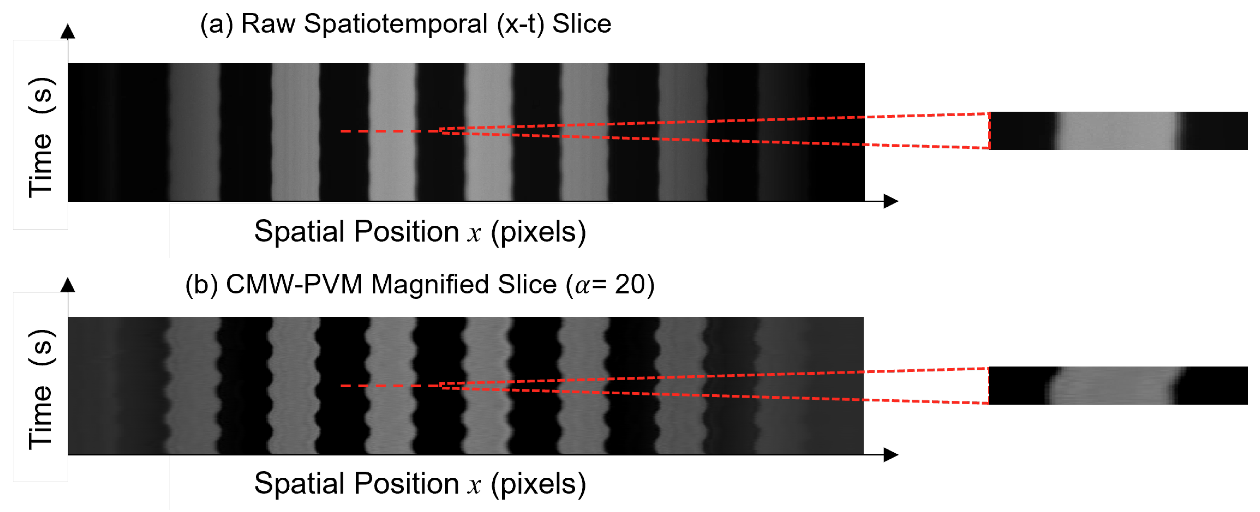
Figure 10 visually compares the $x-t$ cuts of the structural target edge before and after the application of the CMW-PVM algorithm. In the raw unmagnified slice $x-t$ (Figure 10a), the high-contrast edges of the target manifest themselves as perfectly straight horizontal bands. This geometric linearity visually confirms that the physical mechanical vibration of the platform is strictly confined within the sub-pixel regime, rendering the dynamic displacement completely imperceptible to standard optical observation.

In stark contrast, after being processed by the proposed CMW-PVM framework at a magnification factor of $\alpha =20$, the latent micro-vibration is explicitly revealed. As depicted in the magnified $x-t$ slice (Figure 10b), the previously straight edges are transformed into highly visible continuous sinusoidal trajectories. More importantly, close inspection of the wavefronts (see the zoom-in insets) reveals that CMW-PVM faithfully preserves the structural sharpness of the spatial edges. Despite the significant spatial shift, no noticeable ringing artifacts or blurring degradation are introduced, which validates the theoretical findings of high structural fidelity (FSIM) simulated as described in Section 4.4.2.

To quantify the kinematic fidelity of the system, the dynamic displacement trajectory was extracted from the magnified sequence using a sub-pixel edge detection algorithm (normalized by $\alpha$) and compared with the LDV ground truth.

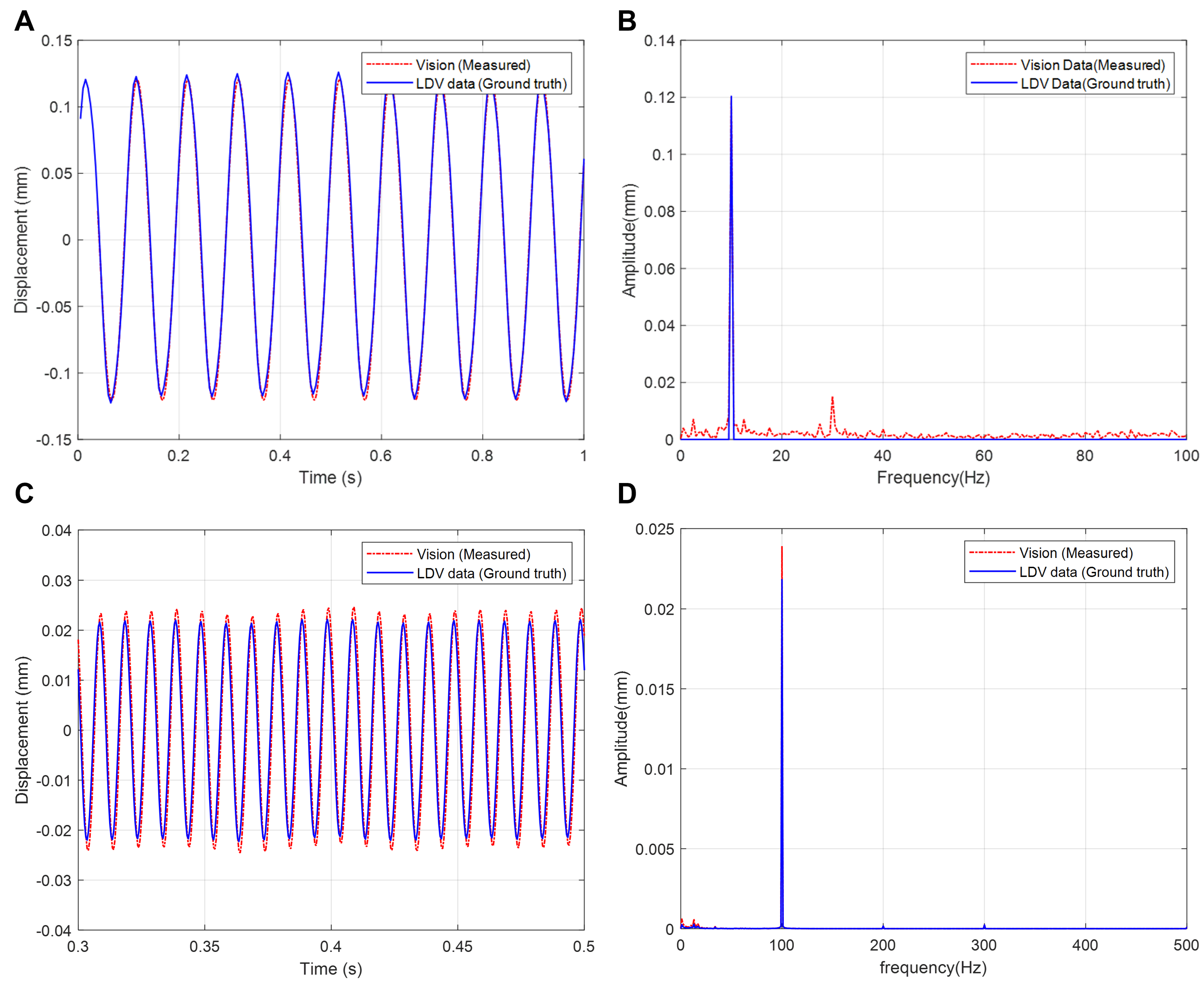
Figure 11A,B present the time-domain overlay and the corresponding fast Fourier transform (FFT) spectrum at a fundamental excitation frequency of 10 Hz. As depicted in the time-domain plot, the vision-extracted trajectory (red dashed line) exhibits high synchronization with the LDV ground truth (blue solid line). The vision system recorded a displacement amplitude of $0.123$ mm compared to the LDV’s $0.121$ mm, resulting in a relative error of $1.65\%$. This correlation confirms that CMW-PVM introduces minimal kinematic distortion during the 1D spatial magnification process for standard vibration frequencies.

Further spectral validation in Figure 11B shows a dominant peak at 10 Hz. The overlapping spectral magnitudes indicate that the energy distribution of the vibration is faithfully preserved. In particular, consistent with the simulation analysis in Section 4.4.2, a minor third-order harmonic component ($3f$ at 30 Hz) is observable in the vision-based spectrum. However, its magnitude remains over 20 dB below the fundamental frequency, indicating that the non-linear distortion is well-controlled.

A critical limitation of traditional vision-based modal analysis using area-scan cameras is the temporal aliasing induced by low frame rates (typically 30–60 fps), which restricts the measurable frequency bandwidth to below 15–30 Hz according to the Nyquist–Shannon sampling theorem. Furthermore, high-frequency vibrations in rigid structures often correspond to diminutive spatial displacements, presenting a dual challenge of temporal resolution and spatial sensitivity.

To demonstrate the bandwidth measurement capability of the proposed line-scan CMW-PVM framework, structural excitation was increased to 100 Hz. As illustrated in Figure 11C, the physical vibration amplitude at 100 Hz drops significantly to approximately $0.022$ mm. Despite the ten-fold increase in frequency and the reduction in the displacement scale, the proposed system successfully reconstructs the rapid sinusoidal oscillations. The vision-based sensor measured an amplitude of $0.024$ mm compared to the LDV reference of $0.022$ mm, maintaining respectable accuracy with a relative deviation of approximately $9.1\%$. This deviation is attributed to the decreased signal-to-noise ratio (SNR) at higher frequencies and smaller amplitudes, yet the waveform integrity remains intact.

The frequency spectrum in Figure 11D correctly identifies the singular peak at 100 Hz without aliasing artifacts. It is important to clarify that this capability does not represent a violation of the Nyquist–Shannon sampling limit; rather, it is achieved by utilizing the high physical line rate of the 1D sensor (configured at 2 kHz in this experiment), which ensures the 100 Hz signal is oversampled and remains well within the folding frequency. This result proves that the system avoids the practical aliasing bottlenecks that plague conventional 30 fps area-scan sensors, effectively extending the operational bandwidth for vision-based metrology.

However, structural health monitoring in industrial settings often involves environmental uncertainties beyond high-frequency demands. While the CMW-PVM framework demonstrates high metrological fidelity under controlled laboratory lighting, its resilience to adverse conditions—specifically illumination fluctuations—requires dedicated evaluation. Since the CMW-PVM algorithm extracts motion from localized phase angles rather than raw pixel intensities, it is theoretically expected to maintain kinematic stability even when the image contrast degrades. To rigorously investigate the engineering robustness of this phase-based architecture, a quantitative stress test under intentionally degraded, low-contrast lighting is presented in the following section.

5.3. Robustness Under Adverse Lighting Conditions

To evaluate the engineering robustness of the CMW-PVM framework beyond controlled laboratory settings, a comparative stress test was conducted. We subjected the system to the same high-frequency configuration validated in Section 5.2 (100 Hz excitation at 0.020 mm amplitude) but intentionally degraded the ambient illumination to simulate a low-contrast, shadow-occluded industrial scenario.

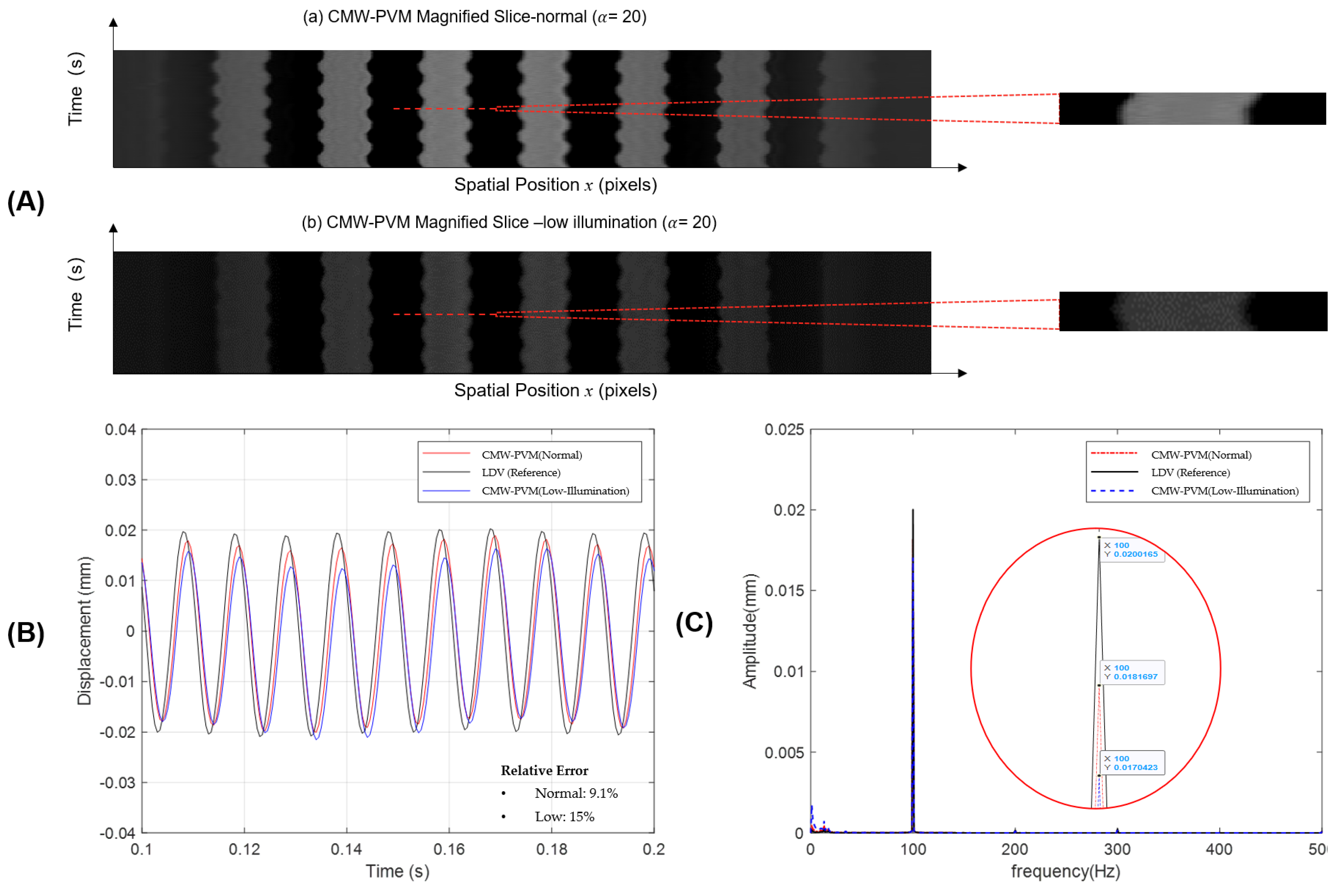
The theoretical resilience of the CMW-PVM algorithm fundamentally lies in its phase-based architecture. As established in Section 3.1, structural vibration is exclusively encoded in the localized phase angle ${\varphi }_{\sigma }$, while sudden lighting drops primarily attenuate the signal’s intensity (amplitude $A_{\sigma }$). Figure 12A visually demonstrates this stability: despite the severe perceptual degradation and increased graininess in the raw $x-t$ spatiotemporal slices under low-light conditions, the fundamental sinusoidal trajectory remains discernible for phase extraction.

Quantitative comparisons between the normal baseline (from Section 5.2) and the low-light stress test are summarized in Figure 12B,C. In the normal environment, the system achieved a measurement of 0.0182 mm (relative error of 9.1%). Under the degraded lighting, the measured amplitude slightly shifted to 0.0170 mm. While the increased background noise introduced minor low-frequency drift—raising the relative amplitude error to 15%—the absolute kinematic error remained tightly bounded at the micrometer scale (≈3 μm). Crucially, as shown in the spectral comparison (Figure 12C), the dominant 100 Hz peak remained perfectly distinct and accurately aligned in both scenarios. This evidence proves that the CMW-PVM localized phase mechanism provides a robust, field-ready solution capable of maintaining metrological integrity in unconstrained, poorly illuminated environments.

Furthermore, while the CMW-PVM framework excels at magnifying periodic vibrations with high precision, its robustness in capturing non-periodic, transient impulses (e.g., impact loading or sudden structural shifts) requires further investigation. Future work will focus on adaptive filtering strategies and potential 1D-to-2D architectural extensions to ensure broader applicability in more diverse and unconstrained industrial environments.

6. Conclusions

This paper presents a 1D-optimized, analytical optical measurement framework designed to accurately capture high-frequency, micro-amplitude structural vibrations. By synergistically combining the ultra-high temporal resolution of line-scan imaging with the robust spatial localization of the proposed Complex Morlet Wavelet Phase-Based Video Magnification (CMW-PVM) algorithm, we address the inherent bandwidth and traceability limitations of conventional 2D vision systems. The primary contributions and findings of this study are summarized as follows.

• 1D-Analytical Metrology Framework: We proposed a novel CMW-PVM framework that establishes a deterministic, analytical mapping between the localized Complex Morlet Wavelet phase and physical structural displacement. By decoupling motion phase from global noise via spatiotemporal localization, the system ensures high kinematic linearity and metrological traceability, complemented by the rigorous derivation of operational boundaries ($\sigma ,\alpha$) to ensure algorithmic stability.
• Superior Robustness in Simulation: Rigorous parametric simulations revealed that CMW-PVM outperforms traditional 1D implementations of EVM and PVM. It extends the dynamic magnification range to $\alpha \approx 35$ and maintains a sub-pixel RMSE baseline with minimal harmonic distortion, demonstrating remarkable noise immunity at SNR $=10$ dB.
• Exceptional Kinematic Accuracy: Physical experiments benchmarked against a high-precision laser Doppler vibrometer (LDV) confirmed the algorithm’s metrological fidelity. At a baseline frequency of 10 Hz, the vision-extracted displacement achieved high synchronization with the ground truth of the LDV, yielding a relative error of only $1.65\%$.
• Broadband and Micro-Displacement Resolvability: The 100 Hz high-frequency experiment explicitly demonstrated the superiority of the line-scan architecture. By leveraging the high physical sampling rate of the 1D sensor, the system effectively avoids the practical aliasing artifacts that typically constrain 30–60 fps area-scan cameras, allowing for the reconstruction of microscopic displacements (≈20 μm) well within the physical Nyquist limits of the hardware.

In conclusion, the proposed line-scan CMW-PVM system provides a highly reliable, cost-effective, and broadband alternative to traditional point-based sensors for industrial structural health monitoring. Beyond vibration metrology, the 1D CMW-PVM framework also holds potential for broader sensing applications that rely on subtle temporal or structural variations. For instance, its noise-resilient localized phase features could support data-driven condition-monitoring pipelines used in air-handling units, where real operational datasets have recently become available [24]. Moreover, the method may complement semi-labeled AHU fault-detection datasets [25] by providing micro-dynamic descriptors that enrich feature representations for mechanical health assessment. In parallel, the rapid development of low-cost optical acquisition platforms [26] suggests promising opportunities for deploying CMW-PVM on compact, field-ready hardware. While the current implementation is restricted to 1D spatial analysis and remains sensitive to extreme illumination fluctuations, addressing these limitations represents a clear direction for enhancement. Future work will focus on improving environmental robustness and deploying the algorithm onto embedded hardware (e.g., FPGA) to achieve real-time, edge-computing-based predictive maintenance for rotating machinery.