Time–Frequency Parallel and Channel-Adaptive Gating for Multivariate Time Series Prediction

Abstract

In real-world scenarios, multivariate time series data typically presents a variety of complex characteristics simultaneously, including long-term trends, multiple seasonality, sudden event disturbances and random noise. Owing to remarkable discrepancies among different variables in dimensions, periodic stability and other aspects, and the gradual evolution of these periodic characteristics over time, models are confronted with numerous challenges in handling non-stationarity, multi-scale dynamic variations and heterogeneous fusion of variables. To tackle these problems, this paper proposes a time–frequency parallel fusion framework—TFDG-Net (Time–Frequency Dual-Branch Gated Fusion Network). This framework models the prior information in the frequency domain and the temporal query network in the time domain in parallel, and introduces a channel-wise gating mechanism to achieve more flexible adaptive fusion after data inverse normalization. Such a design enables the model to operate collaboratively on the original physical scale, which not only improves the long-term prediction capability for periodically stable variables, but also effectively suppresses the interference of noise and event-driven factors, thus significantly enhancing prediction accuracy and the robustness of the training process. In multiple long-term prediction benchmark tests covering fields such as energy and finance, compared with various mainstream models, TFDG-Net reduces the mean squared error and mean absolute error by an average of 12.0% and 7.8% respectively.

1. Introduction

Multivariate time series forecasting (MTSF) plays a pivotal role in numerous critical application domains, encompassing real-world scenarios such as traffic scheduling, financial risk control, industrial process monitoring, power and renewable energy dispatch, and healthcare management [1,2,3]. Unlike natural language or image tasks, real-world time series data generally exhibit the following characteristics: First, they demonstrate significant non-stationarity, manifested as slow drifts in long-term trends and seasonal or cyclical components over time, along with distributional shifts across different stages. Second, time series contain both stable short-term and long-term periodicities, yet are frequently accompanied by event-triggered drastic fluctuations and broadband noise interference. Third, there exists heterogeneity and dynamic coupling among multiple variables; different channels exhibit distinct scales, periodicities, and noise properties [4,5]. These complexities imply that forecasting models must not only possess the capability for accurate extrapolation of long-term cycles but also maintain robustness and adaptability when facing non-periodic disturbances and changes in data distribution [6].

Although various deep learning methods have made progress in their respective dimensions, they still face three universal challenges: First, pure time-domain end-to-end learning often requires the model to independently discover and align periodic structures. When phases drift slowly or amplitudes are modulated by external processes (e.g., weekday/weekend cycles, seasonal transitions, or changes in operating conditions), both training difficulty and sample complexity increase significantly. Second, while performing complex attention mechanisms directly in the frequency domain or simultaneously learning complex spectral magnitudes and phases offers strong expressiveness, such approaches are computationally heavy in both implementation and training. Moreover, phase learning tends to be unstable in the presence of drift and noise. Third, since prior information among multivariate variables is correlated but not universally applicable, a lack of channel-level fine-grained adaptive mechanisms in models can easily lead to over-correction or even performance degradation on channels with weak periodicity or high volatility. The temporal query (TQ) framework provides an effective structural prior for scenarios with strong periodicity: it retrieves query sequences consistent with the input length from a learnable query table via periodic indexing and interacts them with observed features, thereby achieving alignment and template reuse across different phases within the same cycle. TQNet [7], a representative baseline in this direction, relies on temporal queries and cross-channel aggregation to demonstrate robustness across various periodic tasks. However, as it remains confined to the paradigm of time-domain modeling and structural priors, there is still room for improvement when addressing complex scenarios that require frequency-domain extrapolation and explicit correction of periodic errors.

To address the aforementioned challenges, this paper proposes a hybrid time–frequency parallel model designed to exploit frequency-domain priors in a cost-effective and controllable manner while collaborating with a robust time-domain backbone. Specifically, the time-domain pathway employs periodic-indexed temporal query vectors and cross-channel attention to align and reuse periodic patterns. In the frequency-domain pathway, we introduce a frequency-domain correction module: first, a Real Fast Fourier Transform (RFFT) is applied to the input at its original scale, followed by a nonlinear mapping from historical frequency components to predictive ones via a Multilayer Perceptron (MLP) on the magnitude spectrum. The phase spectrum of the input is retained as a prior and paired with the predicted magnitude to reconstruct the complex spectrum for forecasting (phase values for frequency components beyond the historical bandwidth are zero-padded). The corrected complex spectrum is then converted back to the time domain via an Inverse Real Fast Fourier Transform (IRFFT) to yield the correction signal. The two pathways are fused at the original scale: the time-domain output is first denormalized to restore its physical dimensions, then added to the frequency-domain correction signal, with a channel-wise learnable gating mechanism g = σ(γ) introduced to modulate the intensity of frequency-domain injection. The gating is initialized with large negative values to ensure a safe starting state, and during training, it adaptively performs fine-grained channel selection by actively increasing gate values for channels with stable periodicity (e.g., power load, traffic flow, production line rhythms) and reducing them for event-driven or noisy channels (e.g., fault alarms, trading shocks, bursty traffic). This design avoids scaling risks in normalized-space fusion while enhancing interpretability: the magnitude of the gating g can be aligned with the target frequency band energy ratio and the band coherence between the time-domain residual and frequency-domain correction, enabling clear analysis of when and for which variables the model benefits from frequency-domain priors.

The main contributions of this paper are summarized as follows:

(a)

A magnitude-phase decoupling frequency-domain correction module is proposed, which maps only the magnitude spectrum while adopting historical phase values from the input spectrum. New frequency components beyond the historical bandwidth are uniformly zero-padded for completion. This approach stabilizes corrections of periodicity-related errors in the backbone prediction without introducing frequency-domain attention or phase learning.

(b)

Time–frequency fusion is achieved at the original scale through a channel-wise gating mechanism, initialized with low values to ensure stability. During training, the gate dynamically learns channel-specific weights to adjust the intensity of frequency-domain injection according to demand, thereby avoiding over-correction and ensuring robustness.

2. Related Work

2.1. Deep Learning for Time Series Modeling

Early deep learning methods mainly relied on recurrent structures and probabilistic modeling. Autoregressive frameworks based on LSTM and GRU can perform point prediction and interval prediction at the conditional distribution level. Among them, DeepAR maps observation sequences to parameterized distributions for multi-step rolling forecasting, which has been widely validated in scenarios such as e-commerce and energy [8]. On the other hand, convolutional models feature favorable parallelism. TCN enlarges the receptive field while maintaining computational efficiency via dilated convolutions, and has been proven to be highly competitive in capturing short- and medium-term dependencies [9]. In recent years, the paradigm of explicit decomposition and feedforward networks has emerged: N-BEATS parametrically models trend and seasonal components using learnable polynomial and Fourier bases, achieving both interpretability and long-range extrapolation capability [10]. N-HiTS further improves robustness and efficiency through hierarchical interpolation and multi-scale aggregation [11]. To address the inconsistency between training and testing distributions, RevIN performs instance-level reversible normalization and restores the scale at the output end, significantly stabilizing the training process and generalization performance in long-term forecasting tasks across seasons and domains [12].

2.2. Transformer Series

The advantages of Transformers in parallel long-range dependency modeling have spurred numerous time series-adapted variants. Informer proposes ProbSparse attention and a distilling encoder, which significantly reduces spatial–temporal complexity while preserving accuracy, establishing the first strong baseline of efficient attention for long-sequence benchmarks [13]. Autoformer integrates trend–season decomposition with the autocorrelation mechanism, yielding more robust performance in long-period extrapolation [14]. FEDformer further shifts part of the computation to the frequency domain and implements efficient modeling with sparse frequency points and decomposition blocks [15]. Beyond attention sparsification and structural priors, recent works have also highlighted the importance of the variable dimension. PatchTST employs intra-channel independent modeling and cross-channel aggregation, and splits the time axis into patches for representation, achieving prominent gains in Long-Term Time Series Forecasting (LTSF) [16]; iTransformer inverts the token design and emphasizes the expressive capacity of the variable dimension, further advancing performance in multivariate settings [17]. In addition, TimesNet reshapes 1D sequences into multi-period 2D time–frequency variation maps and captures cross-period couplings via convolutions, demonstrating the efficacy of exploiting periodic priors [18].

2.3. Linear Models

Zeng et al. systematically evaluated the effectiveness of Transformers on time series and proposed DLinear and NLinear: after decomposing the problem via simple trend–season decomposition, prediction is accomplished using only a single linear layer, which still achieves or outperforms complex Transformer models on multiple LTSF datasets [19]. This result indicates that the dominant patterns in many data series (especially seasonality) can be sufficiently captured by low-capacity linear modules. DLinear therefore serves as both a strong baseline and a commonly used interpretable linear branch in hybrid models.

2.4. Summary

Existing models suffer from several critical drawbacks: non-stationarity and distribution shift give rise to model mismatch; the evolution of long- and short-term dependencies makes it difficult for a single pathway to balance periodic extrapolation and disturbance suppression; and variable heterogeneity coupled with dynamic coupling leads to over-correction of unified fusion weights. Research by Bernardini et al. has validated the practical feasibility and effectiveness of modeling approaches that integrate frequency-domain modules with neural networks in engineering time series analysis tasks [20]. Therefore, based on TQNet, we organically combine temporal query and cross-channel aggregation with a frequency-domain correction module, and achieve robust fusion at the original scale via channel-wise gating, ultimately obtaining superior performance.

3. Methods

The multivariate time series forecasting problem can be formally defined as follows: Given a historical observation sequence $X_t\in R^{C\times L}$, comprising C variables (or channels) observed over L time steps prior to time step t, the task objective is to generate a prediction sequence $Y_t\in R^{C\times H}$ for the next H future time steps. To address this task, we propose a model named the Time–Frequency Dual-Branch Gated Fusion Network (TFDG-Net).

3.1. Model Overview

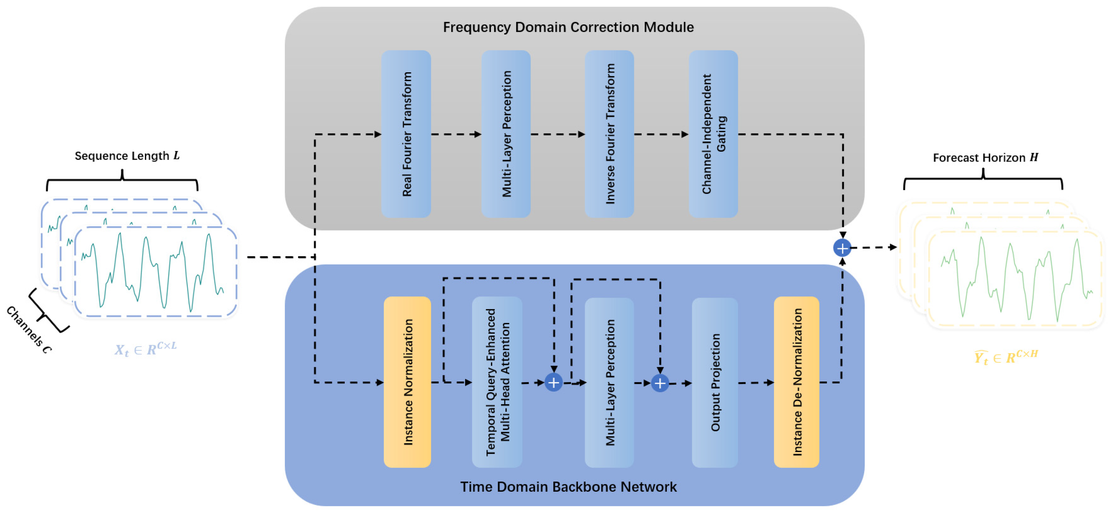
The core idea of TFDG-Net is to decompose the time series forecasting task into two parallel subtasks: temporal dependency modeling and frequency-domain periodicity correction. The overall architecture of the model, as illustrated in Figure 1, consists of four key components:

Input Pre-processing: Instance normalization is applied to mitigate distributional discrepancies across different sequences, enhancing the model’s generalization capability.

Time-Domain Backbone: A network based on multi-head attention and MLP, responsible for directly learning temporal dependencies and dynamic correlations between variables from the input sequence.

Enhanced Frequency Correction Block: Converts the signal to the frequency domain via Fourier transform, learns the evolution patterns of frequency amplitudes using an MLP, and generates a time-domain correction signal.

Channel-wise Gated Fusion Mechanism: Introduces a learnable gating unit to adaptively determine the proportion of frequency-domain correction signals fused for each feature channel, enabling intelligent integration of information.

3.2. Time-Domain Backbone Network

The time-domain backbone network aims to capture local dynamic characteristics of sequences and complex interactions between variables. Its design draws inspiration from the core concept of TQNet, enhancing feature representation capabilities through temporal queries and channel aggregation.

(1)

Temporal Query and Channel Aggregation

We introduce a learnable global temporal query matrix ${\theta }_{tQ}\in R^{W\times C}$, where $W$ is the primary periodic length of the dataset based on prior knowledge (e.g., for hourly power data, $W$ can be 24 or 168). For the $b$-th sample in the batch with starting time index $t_b$, a query vector sequence $Q_b\in R^{L\times C}$ is dynamically extracted through the following modulo operation:

$$\mathrm{i}\mathrm{n}\mathrm{d}\mathrm{e}\mathrm{x}=\left(t_b\left(mod W\right)+\{\mathrm{0,1},\dots ,L-1\}\right)\left(mod W\right)$$

(1)

$$Q_b={\mathsf{\theta }}_{tQ}\left[\mathrm{index}\right]$$

(2)

This query vector $Q$ is fed into a standard multi-head attention module alongside the key ($K$) and value ($V$) vectors generated via linear transformation from the normalized input $X_{\mathrm{norm}}$. The attention computation is defined as

$$\mathrm{Attention}\left(Q,K,V\right)=\mathrm{Softmax}\left({\displaystyle \frac{Q{K}^T}{\sqrt{d_k}}}\right)V$$

(3)

By using globally shared $Q$ and sample-specific $K$, $V$, the attention mechanism effectively smooths out noise and outliers in individual samples when computing inter-channel correlations, thereby learning more stable and generalizable cross-channel dependency patterns.

(2)

Residual MLP Module

The feature representations after channel aggregation are fed into a deep nonlinear module. This module comprises an input projection layer, a core MLP, and an output projection layer, with residual connections widely adopted to stabilize training and prevent information loss. The core MLP contains two linear layers and a GELU activation function, structured as Linear→GELU→Linear, specifically designed to capture temporal dependencies within sequences. Finally, this branch outputs the initial time-domain prediction $Y_{\mathrm{time}}\in R^{B\times H\times C}$.

3.3. Frequency-Domain Correction Module

To explicitly leverage the stable periodicity inherent in time series data, we have designed a frequency-domain correction module. The core hypothesis of this module is that periodic patterns manifest more clearly and stably in the frequency domain, and that future frequency amplitudes can be predicted from historical frequency amplitudes.

(1)

Time-to-Frequency Domain Transformation

The input to this module is a raw historical time series $x\in R^{B\times L_{in}\times C}$, where $B$ denotes the batch size, $L_{in}$ represents the input sequence length, and $C$ corresponds to the number of channels (i.e., variables). To analyze its frequency composition, we first transform the input signal from the time domain to the frequency domain. This process is achieved by applying the Real Fast Fourier Transform (RFFT), which is optimized for real-valued inputs and effectively leverages the conjugate symmetry of the spectrum. The transformation can be formulated as

$$X_{\mathrm{fft}}={\mathcal{F}}_{\mathrm{RFFT}}\left(x\right)$$

(4)

where ${\mathrm{F}}_{\mathrm{R}\mathrm{F}\mathrm{F}\mathrm{T}}(\cdot )$ denotes the RFFT operator. The output $X_{\mathrm{f}\mathrm{f}\mathrm{t}}\in C^{B\times C\times F_{in}}$ is a complex-valued tensor representing the spectrum of the input sequence, with $F_{in}=\lfloor L_{in}/2\rfloor +1$ being the number of non-redundant frequency components determined by the input length. Each complex value $X_{\mathrm{f}\mathrm{f}\mathrm{t}}\left[f\right]$ in the spectrum encodes both the amplitude and phase information corresponding to frequency $f$.

(2)

Nonlinear Mapping of Spectral Magnitudes

We propose a core hypothesis: the evolution of time series is primarily reflected in the redistribution of energy across different frequencies, which directly manifests as changes in the magnitude spectrum in the frequency domain. In contrast, the phase spectrum can be considered relatively stable or inherited from historical phase information in short-term forecasting. Based on this, we decompose the spectrum $X_{\mathrm{fft}}$ into its magnitude $A_{\mathrm{in}}$ and phase ${\mathsf{\Phi }}_{\mathrm{in}}$:

$$A_{in}=\left|X_{\mathrm{fft}}\right|,\hspace{1em}{\mathsf{\Phi }}_{in}=\mathrm{\angle }{X}_{\mathrm{fft}}$$

(5)

To learn the complex mapping from the historical magnitude spectrum $A_{\mathrm{in}}$ to the future magnitude spectrum $A_{\mathrm{pred}}$, we abandon simple linear transformations and instead employ an MLP. This MLP consists of two linear layers and a ReLU activation function, enabling it to model nonlinear dependencies between frequencies, such as energy redistribution, harmonic generation, or attenuation at specific frequencies. The mapping process is defined as

$$A_{pred}=W_2\cdot \mathsf{\sigma }\left(A_{in}\cdot W_1+b_1\right)+b_2$$

(6)

Here, $A_{\mathrm{pred}}\in R^{B\times C\times F_{\mathrm{out}}}$ represents the predicted magnitude spectrum of the future sequence, where $F_{\mathrm{out}}=\lfloor L_{\mathrm{pred}}/2\rfloor +1$ denotes the number of frequency components corresponding to the prediction length $L_{\mathrm{pred}}$, $W_1$ and $b_1$ denote the weight and bias of the first linear layer, while $W_2$ and $b_2$ denote those of the second linear layer.

Compared with existing mainstream frequency-domain processing methods, representative approaches such as FEDformer and TimesNet adopt the joint learning paradigm of the full complex spectrum. They conduct end-to-end synchronous mapping for both the amplitude and phase of the frequency-domain complex spectrum, where both components participate in gradient update and learning, resulting in high modeling complexity. In contrast, the amplitude-spectrum-only mapping method proposed in this paper is formulated as follows:

$$F_{out}=MLP\left(\left|F_{in}\right|\right)\cdot e^{j\cdot \mathrm{\angle }{F}_{in}}$$

(7)

In this method, only the amplitude spectrum $\left|F_{in}\right|$ undergoes nonlinear mapping via MLP, while the phase spectrum $\mathrm{\angle }{F}_{in}$ is directly inherited from the historical observations and does not involve any learning process. This represents a lightweight and robust improvement over existing frequency-domain modeling approaches.

(3)

Spectrum Reconstruction via Phase Reuse

We adopt an efficient reuse strategy for phase information by directly inheriting the phase spectrum of the historical sequence to construct the phase spectrum ${\mathsf{\Phi }}_{\mathrm{resued}}$ of the predicted sequence. The validity of this strategy stems from the fact that phase typically defines the starting position of a waveform, while in many applications, the focus lies on how the intensity (magnitude) of the waveform evolves over time. Using Euler’s formula, we combine the predicted magnitude spectrum $A_{\mathrm{pred}}$ with the reused phase spectrum ${\mathsf{\Phi }}_{\mathrm{resued}}$ to reconstruct the complete future complex spectrum $X_{\mathrm{pred}\_\mathrm{fft}}$:

$$X_{pred\_\mathrm{f}\mathrm{f}\mathrm{t}}=A_{pred}\cdot e^{i\cdot {\mathsf{\Phi }}_{\mathrm{reused}}}$$

(8)

(4)

Frequency-to-Time Domain Inverse Transformation

Finally, the reconstructed complex spectrum $X_{\mathrm{pred}\_\mathrm{fft}}$ is transformed back to the time domain to generate the final prediction correction signal. This process is accomplished by applying the Inverse Real Fast Fourier Transform (IRFFT):

$$Y_{\mathrm{freq}}={\mathcal{F}}_{\mathrm{IRFFT}}^{-1}\left(X_{pred\_fft},n=L_{pred}\right)$$

(9)

where ${\mathrm{F}}_{\mathrm{I}\mathrm{R}\mathrm{F}\mathrm{F}\mathrm{T}}^{-1}(\cdot )$ denotes the IRFFT operator, and the parameter $n=L_{\mathrm{pred}}$ ensures that the length of the output time-domain signal matches the desired prediction horizon $L_{\mathrm{pred}}$. The resulting tensor $Y_{\mathrm{f}\mathrm{r}\mathrm{e}\mathrm{q}}\in R^{B\times L_{\mathrm{pred}}\times C}$ constitutes the final output of this module.

3.4. Channel-Independent Adaptive Gated Fusion

To address the heterogeneity among variables in multivariate time series—where different variables may exhibit distinct periodic and stochastic characteristics—we have designed an adaptive gated fusion mechanism. The core of this mechanism is a learnable, channel-independent gating parameter $g\in R^{1\times 1\times C}$. The outputs of the two branches, $Y_{\mathrm{t}\mathrm{i}\mathrm{m}\mathrm{e}}$ and $Y_{\mathrm{f}\mathrm{r}\mathrm{e}\mathrm{q}}$, are fused as follows:

$$Y_{\mathrm{final}\_\mathrm{norm}}=Y_{\mathrm{time}}+\mathsf{\sigma }\left(g\right)\odot Y_{\mathrm{freq}}$$

(10)

where $\sigma (\cdot )$ denotes the Sigmoid function, which compresses $g$ into the interval $\left(\mathrm{0,1}\right)$ to serve as a dynamic weight for the frequency-domain correction signal, and $\odot$ represents element-wise multiplication implemented via broadcasting.

This design empowers the model to learn a dedicated fusion strategy for each channel. For channels with strong periodicity, the model can optimize the corresponding gating values to approach 1; conversely, for channels dominated by randomness, the gating values are driven towards 0. To guide the training process, we initialize $g$ with negative values. This fusion strategy ensures that during the early stages of training, the model relies primarily on the more easily learned time-domain branch. As the model deepens its understanding of the data structure, it gradually and prudently incorporates the frequency-domain correction information.

4. Experiments and Results

4.1. Experimental Setup

The experiments in this section are implemented based on PyTorch (Paszke et al., 2019) [21], the version number is 2.5.1. The model is optimized using L2 loss and evaluated based on two metrics: mean squared error (MSE) and mean absolute error (MAE). In the experiments, we split the dataset into training, validation and test sets with a fixed ratio of 7:2:1. The datasets used for evaluation and the baseline models are outlined below.

Datasets: We evaluate the proposed method on five widely used real-world datasets, including the ETT series, the Exchange Rate dataset, as well as the Electricity and Weather datasets. These datasets vary in scale, dimensionality (i.e., number of variables), sampling frequency, and application domain. Detailed information about the datasets is provided in

Table 1. Detailed information of the dataset.

Dataset	Channels	Timesteps	Interval	Cycle	Domain
ETTh2	7	14,400	1 h	24	Electricity
ETTm2	7	57,600	15 min	96	Electricity
Weather	21	52,696	10 min	144	Weather
Electricity	321	26,304	1 h	168	Electricity
Exchange	8	7588	1 day	7	Finance

.

Baseline Models: To evaluate the performance of our proposed model, TFDG-Net, we compare it against several representative models from recent years, including TQNet [7], CycleNet [22], iTransformer [17], MSGNet [23], TimesNet [18], PatchTST [16], and DLinear [19]. Following the setup of iTransformer, TFDG-Net defaults to a look-back length of 96.

4.2. Main Results and Analysis

The specific experimental results are as follows.

Table 2. Multivariate time series prediction performance comparison (red indicates the best result, and blue indicates the second-best result).

Model		TFDG-Net (Ours)		TQNet (2025)		CycleNet (2024)		iTransformer (2024)		MSGNet (2024)		TimesNet (2023)		PatchTST (2023)		DLinear (2023)
Metric		MSE	MAE	MSE	MAE	MSE	MAE	MSE	MAE	MSE	MAE	MSE	MAE	MSE	MAE	MSE	MAE
ETTh2	96	0.293	0.343	0.295	0.343	0.298	0.344	0.297	0.349	0.329	0.371	0.340	0.374	0.302	0.348	0.333	0.387
	192	0.371	0.393	0.367	0.393	0.372	0.396	0.380	0.400	0.402	0.414	0.402	0.414	0.388	0.400	0.477	0.476
	336	0.415	0.428	0.417	0.427	0.431	0.439	0.428	0.432	0.440	0.445	0.452	0.452	0.426	0.433	0.594	0.541
	720	0.425	0.442	0.433	0.446	0.450	0.458	0.427	0.445	0.480	0.477	0.462	0.468	0.431	0.446	0.831	0.657
	Avg	0.376	0.402	0.378	0.402	0.388	0.409	0.383	0.407	0.413	0.427	0.414	0.427	0.387	0.407	0.559	0.515
ETTm2	96	0.172	0.254	0.173	0.256	0.163	0.246	0.180	0.264	0.182	0.266	0.187	0.267	0.175	0.259	0.193	0.292
	192	0.238	0.297	0.238	0.298	0.229	0.290	0.250	0.309	0.248	0.306	0.249	0.309	0.241	0.302	0.284	0.362
	336	0.296	0.336	0.301	0.340	0.284	0.327	0.311	0.348	0.312	0.346	0.321	0.351	0.305	0.343	0.369	0.427
	720	0.397	0.395	0.397	0.396	0.389	0.391	0.412	0.407	0.414	0.404	0.408	0.403	0.402	0.400	0.554	0.522
	Avg	0.276	0.320	0.277	0.323	0.266	0.314	0.288	0.332	0.289	0.33	0.291	0.333	0.281	0.326	0.35	0.401
Electricity	96	0.133	0.227	0.134	0.229	0.136	0.229	0.148	0.24	0.165	0.274	0.168	0.272	0.181	0.270	0.197	0.282
	192	0.146	0.242	0.154	0.247	0.152	0.244	0.162	0.253	0.185	0.292	0.184	0.289	0.188	0.274	0.196	0.285
	336	0.155	0.257	0.169	0.264	0.170	0.264	0.178	0.269	0.197	0.304	0.198	0.300	0.204	0.293	0.209	0.301
	720	0.181	0.285	0.201	0.294	0.212	0.299	0.225	0.317	0.231	0.332	0.220	0.320	0.246	0.324	0.245	0.333
	Avg	0.154	0.253	0.164	0.259	0.168	0.259	0.178	0.270	0.194	0.301	0.193	0.295	0.205	0.290	0.212	0.300
Weather	96	0.145	0.192	0.157	0.200	0.158	0.203	0.174	0.214	0.163	0.212	0.172	0.22	0.177	0.210	0.196	0.255
	192	0.186	0.232	0.206	0.245	0.207	0.247	0.221	0.254	0.211	0.254	0.219	0.261	0.225	0.250	0.237	0.296
	336	0.235	0.270	0.262	0.287	0.262	0.289	0.278	0.296	0.273	0.299	0.280	0.306	0.278	0.290	0.283	0.335
	720	0.299	0.318	0.344	0.342	0.344	0.344	0.358	0.349	0.351	0.348	0.365	0.359	0.354	0.340	0.345	0.381
	Avg	0.216	0.253	0.242	0.269	0.243	0.271	0.258	0.278	0.249	0.278	0.259	0.287	0.259	0.273	0.265	0.317
Exchange	96	0.082	0.200	0.083	0.202	0.085	0.203	0.086	0.206	0.102	0.23	0.106	0.234	0.137	0.273	0.088	0.218
	192	0.173	0.295	0.177	0.301	0.178	0.299	0.177	0.299	0.195	0.317	0.227	0.344	0.250	0.370	0.176	0.315
	336	0.324	0.412	0.335	0.419	0.350	0.427	0.331	0.417	0.359	0.436	0.367	0.448	0.446	0.502	0.313	0.427
	720	0.827	0.684	0.913	0.714	0.881	0.703	0.847	0.691	0.940	0.738	0.964	0.746	0.901	0.717	0.839	0.695
	Avg	0.351	0.398	0.377	0.409	0.373	0.408	0.360	0.403	0.399	0.430	0.416	0.443	0.434	0.465	0.354	0.414

summarizes the performance of our model, TFDG-Net, compared to various baseline models across multiple representative datasets. The results clearly demonstrate that TFDG-Net achieves top-two performance in both MSE and MAE across all presented datasets, fully reflecting its overall leading predictive accuracy. Notably, TFDG-Net exhibits superior prediction accuracy on more complex, high-dimensional datasets. For instance, it achieves the best predictive accuracy on both the Weather dataset (21 variables) and the Electricity dataset (321 variables).

Compared to the TQNet model, the performance improvement of TFDG-Net validates the effectiveness of our hybrid time–frequency domain design. Although TQNet effectively models cross-channel dependencies, its pure time-domain architecture still has room for improvement when dealing with data exhibiting strong, stable periodicity (such as Electricity). Our frequency-domain branch provides more accurate periodic predictions for such data by directly extrapolating the frequency spectrum, thereby achieving performance gains.

In comparison with powerful pure time-domain models like iTransformer, the advantage of TFDG-Net lies in its robustness. While Transformer models excel at capturing complex dynamics, they are susceptible to interference from local noise or outliers in the input sequence. The frequency-domain branch of TFDG-Net is insensitive to high-frequency noise and provides a stable baseline prediction. When combined with the dynamic predictions from the time-domain branch, this yields more reliable final results.

4.3. Ablation Studies

To verify the indispensability of each innovative component in TFDG-Net, we conducted a series of ablation experiments. Starting from the full TFDG-Net model, we sequentially removed or replaced its core modules and evaluated the variants on two datasets with distinct characteristics: Weather and Electricity.

Removing the entire frequency-domain branch resulted in a significant drop in predictive accuracy (as shown in

Table 3. TFDG-Net component ablation experiment results (MSE/MAE).

Settings		Without Frequency-Domain Correction, Without Gating		With Frequency-Domain Correction, Without Gating		With Frequency-Domain Correction, With Adaptive Gating		With Frequency-Domain Correction, With Projection Gating
Metrics		MSE	MAE	MSE	MAE	MSE	MAE	MSE	MAE
Weather	96	0.157	0.2	0.147	0.195	0.145	0.192	0.151	0.198
	192	0.206	0.245	0.188	0.234	0.186	0.232	0.193	0.241
	336	0.262	0.287	0.235	0.271	0.235	0.270	0.258	0.288
	720	0.344	0.342	0.300	0.319	0.299	0.318	0.317	0.325
Electricity	96	0.134	0.229	0.138	0.230	0.133	0.227	0.140	0.248
	192	0.154	0.247	0.149	0.244	0.146	0.242	0.152	0.249
	336	0.169	0.264	0.160	0.261	0.155	0.257	0.167	0.263
	720	0.201	0.294	0.189	0.292	0.181	0.285	0.195	0.292

). Compared to our complete TFDG-Net model, the average performance decreased by 12.0% on the Weather dataset and 7.0% on the Electricity dataset. This demonstrates the critical role of frequency-domain correction signals in enhancing prediction accuracy.

Replacing the gated fusion mechanism with simple element-wise addition also led to a decline in performance. Relative to the full TFDG-Net, the average performance dropped by 0.6% on the Weather dataset and 3.4% on the Electricity dataset. This indicates that it is crucial to allow the model to adaptively learn fusion weights for each channel, rather than employing a simple addition strategy. Direct addition may introduce unnecessary noise, particularly in channels lacking strong periodicity.

When the gating mechanism is substituted with linear projection fusion, the model performance likewise deteriorates. Relative to the TFDG-Net model, the average performance decreases by 6.2% on the Weather dataset and by 6.3% on the Electricity dataset, respectively. As a linear structure, the projection gating performs weighted aggregation of all input information, which may result in the forcible incorporation of channel-wise noise into the final prediction. Furthermore, linear architectures are prone to overfitting given limited training data, thereby leading to the degradation of model performance.

4.4. Autonomous Regulation of the Gating Mechanism

To investigate the impact of different gating initialization values on the model, we conducted experiments on the ETTh2 dataset with a prediction length of 96. The results show that the MSE is 0.293 when the initialization value is set to −50, 0.295 for 0, 0.299 for 3, and 0.300 for 10. Since the gating values are computed via the sigmoid function, low negative values cause the gating values to be closer to 0 at initialization. Gating units initialized to be open tend to fit the frequency-domain noise in the training set, leading to overfitting. In contrast, initialization with large negative values activates the gating mechanism only when there is a gain in the frequency domain, which suppresses noise fitting and significantly improves generalization.

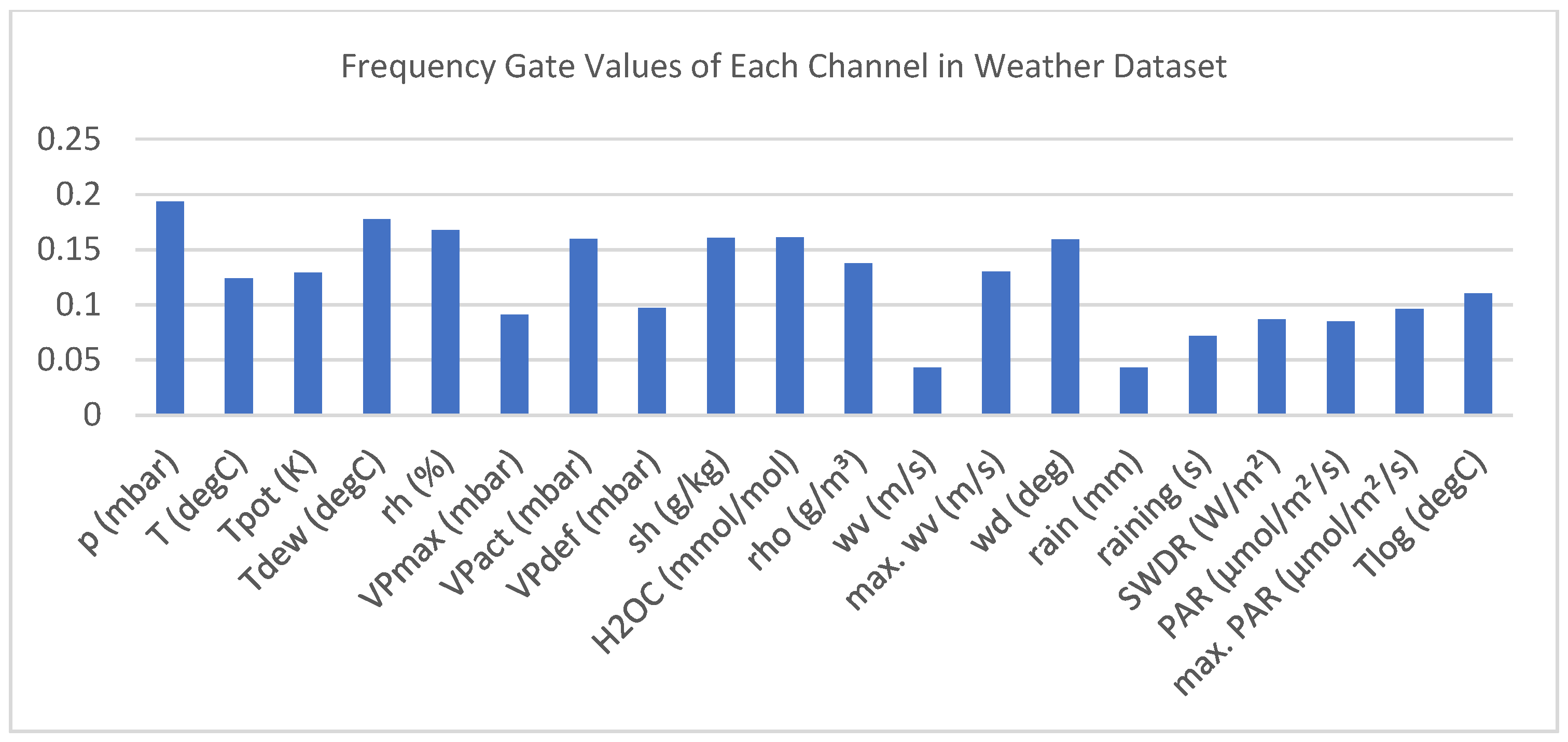
To intuitively understand the operation of the channel-independent gating mechanism, we visualized the learned gating weights $\sigma \left(g\right)$ after training convergence on the Weather dataset, as presented in Figure 2. Overall, we observe that the gating values (frequency gates) primarily serve a corrective function. Rather than drastically altering the predictions generated by the time-domain backbone network, they perform fine-grained adjustments upon this baseline to achieve higher accuracy. This aligns precisely with our objective in incorporating the frequency-domain correction module: to enable the network to adaptively integrate frequency information as needed, without compromising the stability of the backbone.

The gating values are relatively high. Surface pressure sequences exhibit stable semi-diurnal ($\approx$12 h) and diurnal ($\approx$24 h) cycles (atmospheric tides), characterized by minimal phase shifts across seasons and moderate yet stable amplitudes. This strongly aligns with the frequency branch’s hypothesis of “mapping amplitudes while borrowing phases,” resulting in significantly higher gating weights.

Wind Speed and Precipitation: The gating values are lower. Wind speed is heavily influenced by terrain, turbulence, and gusts, exhibiting strong randomness and unstable phases. Precipitation is a typical event-driven sparse sequence that closely resembles broadband noise. Since the frequency branch struggles to reliably extrapolate such signals, the gating mechanism learns to suppress their contribution (approaching zero) to prevent erroneous injection.

4.5. Phase Strategy Analysis

To verify the rationality of the proposed phase reuse strategy, this section compares the prediction performance of three typical phase handling strategies. The experimental results are shown in

Table 4. Comparative analysis of phase strategies.

Phase Strategy	Phase Reuse		Zero-Phase Padding		Full Complex Spectrum Learning
Metric	MSE	MAE	MSE	MAE	MSE	MAE
Weather	0.145	0.192	0.148	0.190	0.149	0.191
Electricity	0.133	0.227	0.134	0.226	0.134	0.226
ETTh2	0.293	0.343	0.295	0.345	0.305	0.348

, where the prediction length is uniformly set to 96. It can be observed from the table that the phase reuse strategy achieves the optimal performance among the three strategies. Zero-phase padding directly fills zeros for newly added frequency components, which disrupts phase continuity and periodic alignment, introduces spectral leakage and reconstruction artifacts, and results in a slight degradation of prediction accuracy. This impact is more pronounced on the phase-sensitive ETTh2 dataset. Full complex spectrum learning necessitates simultaneous phase learning. However, phase is characterized by strong nonlinearity and high noise sensitivity, making it arduous to learn and prone to overfitting. Furthermore, for period-dominated time series data, phase only determines the starting position of the waveform, while the core information is dominated by magnitude. Phase learning constitutes redundant modeling, which conversely interferes with the effective learning of magnitude, thus leading to inferior performance relative to phase reuse.

4.6. Efficiency Analysis

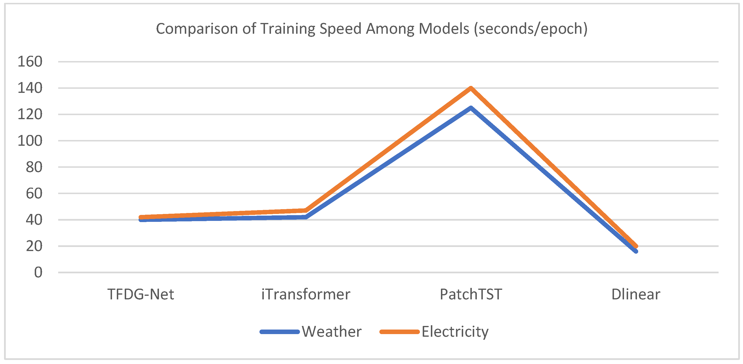
Our hardware environment consists of an Intel Core Ultra 5 125H CPU (Intel Corporation, Santa Clara, CA, USA), an NVIDIA RTX 4060 (8 GB) GPU (NVIDIA Corporation, Santa Clara, CA, USA), and 32 GB of memory. The prediction horizon is set to 720, and the detailed experimental results are presented in Figure 3. The per-epoch training time of TFDG-Net is lower than that of iTransformer and PatchTST, and only higher than that of the purely linear model DLinear. The time-domain backbone of TFDG-Net adopts an MLP architecture, whose core computations originate from input projection, two layers of nonlinear MLP, and output projection, with a time complexity of $\mathcal{O}\left(L\cdot C+d_{model}^2\right)$ (where $L$ denotes the input sequence length, $C$ denotes the number of channels, and $d_{model}$ denotes the hidden dimension). The channel attention module employs a 4-head multi-head attention mechanism, which performs feature aggregation solely along the channel dimension without global self-attention in the temporal dimension, thus avoiding the high O($L^2$) complexity inherent to Transformer-based models. Temporal queries are learnable parameters that implement periodic modeling only via indexing and broadcasting operations, resulting in negligible computational overhead. The core computations of the frequency-domain module are FFT/IRFFT and MLP, where the time complexity of FFT/IRFFT is $\mathcal{O}\left(L\log L+H\log H\right)$. The frequency-domain MLP is a two-layer linear structure with an input dimension of $F_{in}=L/2+1$ (only half of the input sequence length) and a hidden layer dimension of $\left(F_{in}+F_{out}\right)/2$.

5. Limitations

The performance of TFDG-Net heavily relies on the assumption of frequency-domain stationarity of signals, which still imposes limitations on its application to certain extreme scenarios. In chaotic dynamic systems such as severe convective weather or high-frequency turbulence, the data often lack stable evolutionary laws, and the scattered spectral distribution makes it difficult for MLP-based mapping operators to capture effective patterns. Furthermore, the phase reuse strategy is essentially a prior based on physical inertia. Once the sequence undergoes severe phase shift or is disturbed by noise, reusing historical phases will instead cause destructive interference with the time-domain signal, even introducing spectral artifacts and impairing prediction accuracy. To tackle these challenges, the channel adaptive gating mechanism we designed serves as a safety net: when frequency-domain prediction fails, the model can automatically switch to the robust time-domain backbone, thereby safeguarding the bottom line of performance. In future work, we will introduce tools such as dynamic phase compensation and wavelet transform to enhance the extraction of non-stationary features, and explore a lightweight paradigm via sparse sampling to meet the deployment requirements of edge monitoring devices.

6. Conclusions

Addressing the challenges in current multivariate time series forecasting tasks regarding periodic feature mining, scale matching for cross-branch information fusion, and adaptation to variable heterogeneity, this paper proposes a Time–Frequency Hybrid Parallel Modeling Framework. This framework establishes a robust time-domain backbone based on time queries and cross-channel aggregation. In parallel, it incorporates a frequency-domain correction module: it applies the Real Fast Fourier Transform (RFFT) to the input at its original scale, learns a nonlinear mapping from historical frequency bins to predicted ones via an MLP exclusively on the amplitude spectrum, retains the phase from the input spectrum, and completes components beyond the historical band with zero phase. These are combined to obtain the predicted complex spectrum, which is then restored to a time-domain correction signal via the Inverse RFFT (IRFFT). To ensure robust fusion and interpretability, we perform post-fusion at the original scale and introduce a channel-wise learnable gating mechanism. We adopt a safer initialization strategy that suppresses the frequency branch during early training and adaptively activates it as data learning progresses, thereby actively injecting corrections into channels with stable periodicity while automatically shrinking contributions from noisy or event-driven channels. TFDG-Net demonstrates superior performance across five challenging real-world datasets, fully showcasing the model’s effectiveness and practicality in solving complex multivariate time series forecasting problems in the real world.

References

1. Hochreiter, S.; Schmidhuber, J. Long short-term memory. Neural Comput. 1997, 9, 1735–1780. [Google Scholar] [CrossRef] [Scilit] [PubMed]
2. Lai, G.; Chang, W.-C.; Yang, Y.; Liu, H. Modeling long-and short-term temporal patterns with deep neural networks. In Proceedings of the 41st International ACM SIGIR Conference on Research & Development in Information Retrieval, Ann Arbor, MI, USA, 8–12 July 2018; pp. 95–104. [Google Scholar]
3. Wang, Y.; Wu, H.; Dong, J.; Liu, Y.; Long, M.; Wang, J. Deep Time Series Models: A Comprehensive Survey and Benchmark. arXiv 2024, arXiv:2407.13278. [Google Scholar] [CrossRef] [Scilit]
4. Pantiskas, L.; Verstoep, K.; Bal, H. Interpretable Multivariate Time Series Forecasting with Temporal Attention Convolutional Neural Networks. In Proceedings of the 2020 IEEE Symposium Series on Computational Intelligence (SSCI), Canberra, ACT, Australia, 1–4 December 2020; pp. 1687–1694. [Google Scholar] [CrossRef] [Scilit]
5. Yi, K.; Zhang, Q.; Fan, W.; Cao, L.; Wang, S.; He, H.; Long, G.; Hu, L.; Wen, Q.; Xiong, H. A Survey on Deep Learning based Time Series Analysis with Frequency Transformation. In Proceedings of the 31st ACM SIGKDD Conference on Knowledge Discovery and Data Mining, New York, NY, USA, 3–7 August 2025; pp. 6206–6215. [Google Scholar] [CrossRef] [Scilit]
6. Wang, Y.; Wu, H.; Dong, J.; Qin, G.; Zhang, H.; Liu, Y.; Qiu, Y.; Wang, J.; Long, M. TimeXer: Empowering transformers for time series forecasting with exogenous variables. In Proceedings of the 38th Annual Conference on Neural Information Processing Systems (NeurIPS 2024), Vancouver, BC, Canada, 8–14 December 2024. [Google Scholar]
7. Lin, S.; Chen, H.; Wu, H.; Qiu, C.; Lin, W. Temporal Query Network for Efficient Multivariate Time Series Forecasting. arXiv 2025, arXiv:2505.12917. [Google Scholar] [CrossRef] [Scilit]
8. Salinas, D.; Flunkert, V.; Gasthaus, J.; Januschowski, T. DeepAR: Probabilistic forecasting with autoregressive recurrent networks. Int. J. Forecast. 2020, 36, 1181–1191. [Google Scholar] [CrossRef] [Scilit]
9. Bai, S.; Kolter, J.Z.; Koltun, V. An empirical evaluation of generic convolutional and recurrent networks for sequence modeling. arXiv 2018, arXiv:1803.01271. [Google Scholar] [CrossRef] [Scilit]
10. Oreshkin, B.N.; Carpov, D.; Chapados, N.; Bengio, Y. N-BEATS: Neural basis expansion analysis for interpretable time series forecasting. arXiv 2019, arXiv:1905.10437. [Google Scholar]
11. Challu, C.; Olivares, K.G.; Oreshkin, B.N.; Ramirez, F.K.; Canseco, M.M.; Dubrawski, A. Nhits: Neural hierarchical interpolation for time series forecasting. In Proceedings of the 37th AAAI Conference on Artificial Intelligence, Washington, DC, USA, 7–14 February 2023. [Google Scholar]
12. Kim, T.; Kim, J.; Tae, Y.; Park, C.; Choi, J.H.; Choo, J. Reversible instance normalization for accurate time-series forecasting against distribution shift. In Proceedings of the International Conference on Learning Representations (ICLR 2022), Virtual, 25–29 April 2022. [Google Scholar]
13. Zhou, H.; Zhang, S.; Peng, J.; Zhang, S.; Li, G.; Mei, H.; Ma, H.; Wen, Q. Informer: Beyond efficient transformer for long sequence time-series forecasting. In Proceedings of the 35th AAAI Conference on Artificial Intelligence, Virtual, 2–9 February 2021. [Google Scholar]
14. Wu, H.; Xu, J.; Wang, J.; Long, M. Autoformer: Decomposition transformers with auto-correlation for long-term series forecasting. Adv. Neural Inf. Process. Syst. 2021, 34, 22419–22430. [Google Scholar]
15. Zhou, T.; Ma, Z.; Wen, Q.; Wang, X.; Sun, L.; Jin, R. Fedformer: Frequency enhanced decomposed transformer for long-term series forecasting. In Proceedings of the 39th International Conference on Machine Learning, Baltimore, MD, USA, 17–23 July 2022. [Google Scholar]
16. Nie, Y.; Nguyen, N.H.; Sinthong, P.; Kalagnanam, J. A Time Series is Worth 64 Words: Long-term Forecasting with Transformers. arXiv 2022, arXiv:2211.14730. [Google Scholar]
17. Liu, Y.; Hu, T.; Zhang, H.; Wu, H.; Wang, S.; Ma, L.; Long, M. itransformer: Inverted transformers are effective for time series forecasting. arXiv 2023, arXiv:2310.06625. [Google Scholar]
18. Wu, H.; Hu, T.; Liu, Y.; Zhou, H.; Wang, J.; Long, M. Timesnet: Temporal 2D-variation modeling for general time series analysis. arXiv 2022, arXiv:2210.02186. [Google Scholar]
19. Zeng, A.; Chen, M.; Zhang, L.; Xu, Q. Are transformers effective for time series forecasting? In Proceedings of the 37th AAAI Conference on Artificial Intelligence, Washington, DC, USA, 7–14 February 2023. [Google Scholar]
20. Bernardini, L.; Bono, F.M.; Collina, A. Drive-by damage detection and localization exploiting continuous wavelet transform and multiple sparse autoencoders. Railw. Eng. Sci. 2025, 33, 721–745. [Google Scholar] [CrossRef] [Scilit]
21. Paszke, A.; Gross, S.; Massa, F.; Lerer, A.; Bradbury, J.; Chanan, G.; Killeen, T.; Lin, Z.; Gimelshein, N.; Antiga, L.; et al. PyTorch: An Imperative Style, High-Performance Deep Learning Library. In Proceedings of the 33rd International Conference on Neural Information Processing Systems, Vancouver, BC, Canada, 8–14 December 2019; Curran Associates Inc.: Red Hook, NY, USA, 2019; pp. 8026–8037. [Google Scholar]
22. Lin, S.; Lin, W.; Hu, X.; Wang, S. Cyclenet: Enhancing time series forecasting through modeling periodic patterns. Adv. Neural Inf. Process. Syst. 2024, 37, 106315–106345. [Google Scholar]
23. Cai, W.; Liang, Y.; Liu, X.; Feng, J.; Zhou, K. Msgnet: Learning multi-scale inter-series correlations for multivariate time series forecasting. In Proceedings of the 38th AAAI Conference on Artificial Intelligence, Vancouver, BC, Canada, 20–27 February 2024. [Google Scholar]
Figure 1. TFDG-Net model structure.
Applsci 16 03266 g001
Figure 2. Frequency gate values of each channel in Weather dataset.
Applsci 16 03266 g002
Figure 3. Comparison of training speed among models (seconds/epoch).
Applsci 16 03266 g003