NIR Spectroscopy and Machine Learning for the Quantification of Blended Textiles: Towards Improved Understanding for Textile Recycling

Abstract

Accurate quantification of cotton content is a key prerequisite for efficient textile recycling. However, it remains challenging due to material heterogeneity and technical limitations. Near-infrared spectroscopy (NIR) combined with advanced data analysis offers a rapid, non-destructive approach. However, systematic evaluations across instrument classes and analysis strategies for industrial textile sorting remain limited. In this study, a unique set of cotton/polyester blends from the same starting material with varying cotton content was analyzed using three NIR systems representing laboratory, handheld, and industrial sensor-based applications. Multiple spectral preprocessing strategies were systematically combined with partial least squares regression and advanced machine learning models. Model performance was evaluated using cross-validation and independent test sets. The benchtop NIR system delivered the highest and most consistent performance, achieving RMSEP values below 1.0% with advanced regression models. The handheld and imaging sensor system exhibited higher RMSEP values (1.2–1.6%), reflecting not only differences in preprocessing and model selection, but also intrinsic instrumental limitations. Overall, the results demonstrate that each NIR instrument class exhibits distinct strengths and limitations with respect to accuracy, sensitivity, and robustness. Consequently, instrument-specific preprocessing, models, and hyperparameters are required, and no universally transferable pipeline was identified.

1. Introduction

Textile waste is a growing environmental issue due to the resource-intensive nature of textile production and the fast fashion industry [1]. Global fiber production has almost doubled over the past two decades, rising from 58 million tones in 2000 to 134 million tones in 2024 [2]. During this period, textile production more than doubled, while the average lifespan decreased by around 40% before disposal [3,4]. This challenge is expected to intensify, as the textile industry increasingly operates on microtrend-driven models that rely on rapid, linear production processes to satisfy the volume of rising sales [5,6]. All these trends have resulted in a significant amount of textile waste, most of which ends up in incinerators or landfill sites [3]. Due to this, it is estimated that the textile industry represents the fourth most significant environmental impact, following the housing, transport, and food sectors [7]. As part of the European Green Deal, the EU has outlined targets aimed at promoting sustainable textile management, particularly in response to the challenges posed by fast fashion trends [8]. The growing demand for recycling is further driven by heightened awareness of environmental degradation, resource scarcity, and the need to reduce pollution [9].

Efficient recycling requires a focus on the most prevalent fiber types. Among these, cotton and polyester are the most widely used [9,10,11,12,13,14]. This is due to their ability to combine the desirable properties of both fibers. While cotton contributes softness, breathability, and comfort, polyester enhances durability, wrinkle resistance, and dimensional stability, resulting in versatile and high-performance fabrics [9,10,11,12,15]. However, recycling cotton/polyester blends remains challenging due to the difficulty of separating the two fiber types. Various strategies—including mechanical, chemical, and biological methods—have been explored to facilitate the separation of blended fibers. Also, pretreatments such as mechanical shredding or alkaline washing are commonly used [15]. In this study, an enzymatic approach was employed to separate cotton/polyester blends [16]. During process development, one of the critical aspects is the identification of a fast and reliable method for quantifying the cotton content in blended textiles in the input material.

Nowadays, vibrational techniques are widely used in various applications. In this work, we focus on near-infrared (NIR) spectroscopy as a fast, easy-to-use, low-cost, and environmentally friendly method for cotton quantification, which has been applied across diverse analytical fields, including agriculture, medicine, and the chemical industry [17,18,19]. Also, in the textile industry, NIR spectroscopy is used for a vast number of (analytical) questions [20], for example, for sorting as a classification method. Its capability to efficiently and accurately recognize different textile fibers outperforms that of other identification methods [21,22], especially in combination with advanced data analysis methods like machine learning tools [23,24,25]. It has also been employed for the characterization and identification of cellulose-based materials, including cotton and regenerated cellulose [15,26], as well as for the prediction of quality parameters such as the Micronaire value [27]. For the quantification of cotton in fiber blends (e.g., cotton/polyester), cotton exhibits characteristic absorption bands of cellulose in the NIR region that can be used for compositional analysis [28]. Characteristic absorption bands appear at 8230–8000 cm⁻¹, corresponding to the second overtone of C–H/O–H stretching vibrations, as well as at 6712 cm⁻¹ and 4739 cm⁻¹, both attributed to combined O–H stretching and bending vibrations [9]. Polyester (PET), on the other hand, exhibits absorption bands at 6100–6000 cm⁻¹, associated with the first overtone of –CH and –CH₂ vibrations, and around 5800 cm⁻¹, corresponding to the second overtone of the carbonyl group [14]. These features were successfully used in the past to create models for prediction of the cotton content. For example, Ruckebusch et al. used a combination of partial least squares (PLS) regression and genetic algorithms for wavelength selection to predict the cotton content of cotton/silk blends using a benchtop NIR instrument, achieving an error rate of around 2% [29]. This was confirmed by Paz et al., who achieved error rates of around 3% for NIR and 6% for MIR in the prediction of the cotton content in cotton/polyester blends [14]. Also, Chen et al. predicted the cotton content using NIR in clothes samples to replace labor-intense and time-consuming methods [30]. Handheld and hyperspectral imaging instruments have also been successfully employed for the quantification of cotton [26,31]. However, these methods typically exhibit higher error rates compared to benchtop NIR instruments [31].

For quantitative analysis, preprocessing techniques—which can significantly enhance the performance of calibration models [32,33]—are commonly applied. Such preprocessing typically aims to compensate for scatter effects, path length differences, and other low-frequency spectral variations rather than to perform classical baseline correction. Among regression approaches, PLS regression remains the most widely used method across various fields [7,14,20,31,34,35], although more complex machine learning models have been shown to outperform PLS under certain conditions [36,37,38,39]. Moreover, the effectiveness of spectral preprocessing and regression models is known to be strongly dependent on instrument-specific characteristics such as spectral resolution, signal-to-noise ratio, and accessible wavelength ranges, highlighting the need for instrument-aware data analysis strategies.

It is evident that machine learning regression methods are of particular significance in accelerating and enhancing the analysis of samples [40]. However, systematically comparing preprocessing strategies and regression approaches in a chemically meaningful framework remains challenging, particularly when expert knowledge is required to ensure interpretability, robustness, and transferability in textile applications. This is particularly notable given that the No Free Lunch Theorem, a foundational principle in machine learning, posits that one cannot presume, in advance, the suitability of a particular model for a given task [41]. Consequently, a structured and comprehensive evaluation framework is required to assess not only predictive accuracy, but also robustness, overfitting behavior, and generalization across instrument types.

In this study, we systematically compare the performance of different NIR instrument classes for the quantification of cotton content in blended textiles and analyze how model complexity and spectral preprocessing interact with instrument-specific characteristics. This evaluation is framed within the context of the No Free Lunch Theorem, which states that no single regression approach can be expected to perform optimally across all datasets. Textile materials are inherently heterogeneous systems. Beyond chemical composition (fibers, dyes, finishing agents), physical properties such as color, thickness, and surface structure introduce substantial spectral variability. These factors affect reflectance and scattering behavior and can significantly influence model robustness and transferability. To isolate methodological effects and systematically evaluate interactions under controlled conditions, we acquired a large dataset of over 200 samples from the same source material, but with varying cotton content derived from an enzymatic recycling process, using three different spectroscopic instruments that differ in terms of spectral resolution, sensitivity, and the used wavenumber range. The acquired spectra were subjected to six preprocessing techniques and five regression models, enabling a systematic investigation of model performance. The evaluation criteria of the models included statistical performance metrics (e.g., R², RMSE), the interpretability of the resulting feature importance, and computational efficiency (training time).

2. Materials and Methods

2.1. Description of the Dataset Used

Enzymatic hydrolysis was used to prepare a total of 200 fabric samples derived from the same 50/50 cotton/polyester base material (white plain weave bedsheet, 140 g/m²) sourced from Salesianer Miettex GmbH, Vienna, Austria. The samples were processed in batches of 20 pieces (sample size 40 × 40 cm each) per hydrolysis experiment, resulting in ten treatment batches. Within each batch, identical reaction conditions were applied, while enzyme activity levels were varied between batches to obtain fabrics with different cotton/polyester ratios. Before enzymatic treatment, fabrics were prewashed with 2% on a weight of fabric (owf) sodium carbonate solution (liquor ratio 1:10) at 60 °C for 30 min and rinsed until neutral. Hydrolysis experiments were carried out in an enclosed reactor system with controlled heating and agitation at a liquor ratio of 1:10 in a 20 mM sodium citrate buffer (pH = 6) for 4 h. The enzyme formulation used remained consistent and was a commercial cellulase product from NewEnzymes, Pedrouços, Portugal.

The cotton content of the original fabric was confirmed by treating five samples with concentrated sulfuric acid (75 wt%; Merck, Darmstadt, Germany) for 1 h at 50 °C with agitation every 10 min to dissolve the cellulosic portion of the blend, according to ISO 1833-11 [42]. The cotton content remaining after enzymatic hydrolysis was determined through gravimetric analysis, which is typical for enzymatic hydrolysis studies [43]. The weight loss after an enzymatic treatment was assumed to be entirely cotton weight loss since the enzymes do not interact with the PET component. The new cotton/polyester blend ratio was calculated using the original weight of PET and reduced weight of cotton after hydrolysis.

The dataset covered a cotton content range of 28.9–50.0%, with a mean value of 39.8% (±5.0%). The interquartile range (36.7–42.6%) indicates a balanced distribution of cotton fractions around the median (39.5%), suitable for robust calibration and validation of regression models. The distribution of reference ratios is shown as a violin plot in the Supplementary Materials (Figure S1). The intentionally controlled compositional range and the use of single-source material reduce external variability arising from differences in fabric structure, dyeing, or finishing treatments. This design enables a systematic investigation of instrument- and model-related effects under defined laboratory conditions while not aiming to represent the full heterogeneity of post-consumer textile waste.

2.2. Infrared Spectroscopy

All samples were measured using three different NIR instruments, each with varying performance in terms of wavelength range, sensitivity, and spectral resolution. These included a high-performance benchtop NIR spectrometer (Bruker Optics GmbH, Ettlingen, Germany), a handheld instrument, and an NIR imaging sensor system (

Table 1. Overview of the instruments used for NIR measurement. Further details are mentioned in the text. Since the use of the wavenumber is common in R&D spectrometers, no conversion has been made here.

Instruments	Details	Wavelength Range	Spectral Resolution
Benchtop NIR	Bruker MPA	12,500–4000 cm−1	4 cm−1
Handheld NIR	microPhazirTM NIR spectrometer	1596–2396 nm	8 nm
Imaging sensor system	Binder + Co AG	911–1677 nm	9 nm

). For the handheld and benchtop instruments, each specimen was measured five times on random spots.

The benchtop NIR was used with an InGaAs detector exhibiting linear sensitivity throughout the full wavenumber range. The diffuse reflectance measurements were conducted with a rotating sample stage of approximately 10 cm in diameter. Background measurements were performed with a gold stamp. Each spectrum was acquired as the average of 16 scans. For point-based spectral measurements, a handheld NIR spectrometer—microPhazir™ from Thermo Fisher Scientific (Waltham, MA, USA)—was employed [44]. This instrument operates based on diffuse reflectance and captures spectral data over a spot size of around 4 mm, with a spectral resolution of 8 nm per pixel. Measurements were performed using the manufacturer’s default acquisition settings, corresponding to an integration time of approximately 1–2 s per spectrum. In comparison, the NIR sorting system (Binder + Co AG, Gleisdorf, Austria) incorporates the Helios NIR G2-320 hyperspectral imaging sensor (EVK DI Kerschhaggl GmbH, Raaba, Austria), which records 312 spectral channels (detector pixels) across the measured wavelength range, with a spectral resolution of approximately 9 nm [45]. The integration time was optimized during system calibration to ensure appropriate signal intensity and was kept constant for all measurements (1.8 ms). This imaging sensor (camera) is identical to that used in industrial sensor-based sorting systems. In contrast to industrial sorting units, where material is transported on a horizontal conveyor belt, the laboratory setup employed an inclined sliding conveyor to allow for controlled image acquisition of the samples.

Depending on the literature and the instrument used, spectral features are reported either in wavenumber (cm⁻¹) or the wavelength (nm). For clarity, we used the wavenumber (cm⁻¹) throughout this document.

2.3. Data Analysis

Before data analysis, including preprocessing, the spectral range of the benchtop NIR was limited to 3800–7800 cm⁻¹. For the handheld NIR and sensor imaging system, the whole spectral range was used. Spectral preprocessing was performed using the following methods: Standard Normal Variate transformation, detrending with polynomial degree of 2, fillPeaks (λ = 1, half window interval = 10, 6 iterations, intensity threshold = 400), and Savitzky–Golay filter with first derivative polynomial order three and varying window size. Also, a combination of the selected preprocessing methods was tested. All preprocessing steps were conducted using the statistical software R (v4.5.1) and the spectral processing libraries prospectr (v0.2.8) and baseline (v1.3-7).

Based on preliminary results [46], a total of five regression models were evaluated to predict the cotton content from preprocessed spectral data. Partial least squares (PLS) regression was used as a reference predictive model. It represents the standard approach in vibrational spectroscopic analysis due to its robustness against multicollinearity and high-dimensional data. To benchmark the performance, nonlinear machine learning models were additionally considered, including kernel ridge regression with a polynomial kernel (KRR), random forest regression (RF), least squares support vector machines (LS-SVM), and the gradient-boosting-based XGBoost algorithm. All computations were performed in Python (v3.10.8) using custom scripts and standard machine learning libraries, including scikit-learn version 1.6.1. Possible outliers were identified and removed based on residual analysis and visual inspection of predicted versus measured plots.

Model development followed a two-stage validation strategy designed to strictly separate hyperparameter optimization from final model evaluation. First, the dataset was divided into a training set (75%) and an independent test set (25%) using a specimen-oriented grouping strategy, ensuring that all measurements from the same specimen were assigned exclusively to either the training or test set. This prevented data leakage between calibration and test data. Hyperparameter optimization was performed exclusively on the training data using a random search on a combination of hyperparameters (RandomizedSearchCV) with four-fold grouped cross-validation and forty randomized hyperparameter configurations per model. The four-fold cross-validation procedure was repeated ten times with different random fold assignments. Consequently, with four folds, ten repetitions and forty randomly sampled hyperparameter configurations per model, a total of 1600 internal model fits per algorithm were performed.

After identifying the optimal hyperparameter combination, the final model was refitted using the entire training set and then evaluated using the independent test set, which remained entirely unseen during the tuning process. Model performance is reported using chemometric terminology to distinguish between RMSEC (root mean squared error of calibration, calculated on the training set) and RMSEP (root mean squared error of prediction, calculated on the independent test set), together with the corresponding R² values. This validation strategy ensures that hyperparameter selection does not bias the reported predictive performance, enabling transparent comparison between calibration, cross-validation, and independent prediction results. Hyperparameter spaces were tailored to each model, including polynomial degree and regularization strength for kernel ridge regression, tree depth and ensemble size for Random Forest, number of components for PLS, and kernel parameters for LS-SVM (Supplementary Materials, Table S1).

Feature relevance was assessed using two complementary approaches. For partial least squares (PLS) regression, variable importance was evaluated based on the model loadings, which directly reflect the contribution of individual spectral variables to the latent components. For XGBoost, feature importance scores were calculated based on the contribution of individual features to the model’s decision process. Due to the strong collinearity inherent to vibrational spectroscopic data, feature importance measures derived from ensemble methods such as random forest are known to be biased and difficult to interpret physically. In addition, LS-SVM and kernel ridge regression operate in an implicit kernel-induced feature space and do not provide direct weights for individual spectral variables. Consequently, these models were used exclusively for predictive performance assessment.

3. Results and Discussion

3.1. Instrument-Dependent NIR Spectral Features and Influence of Preprocessing

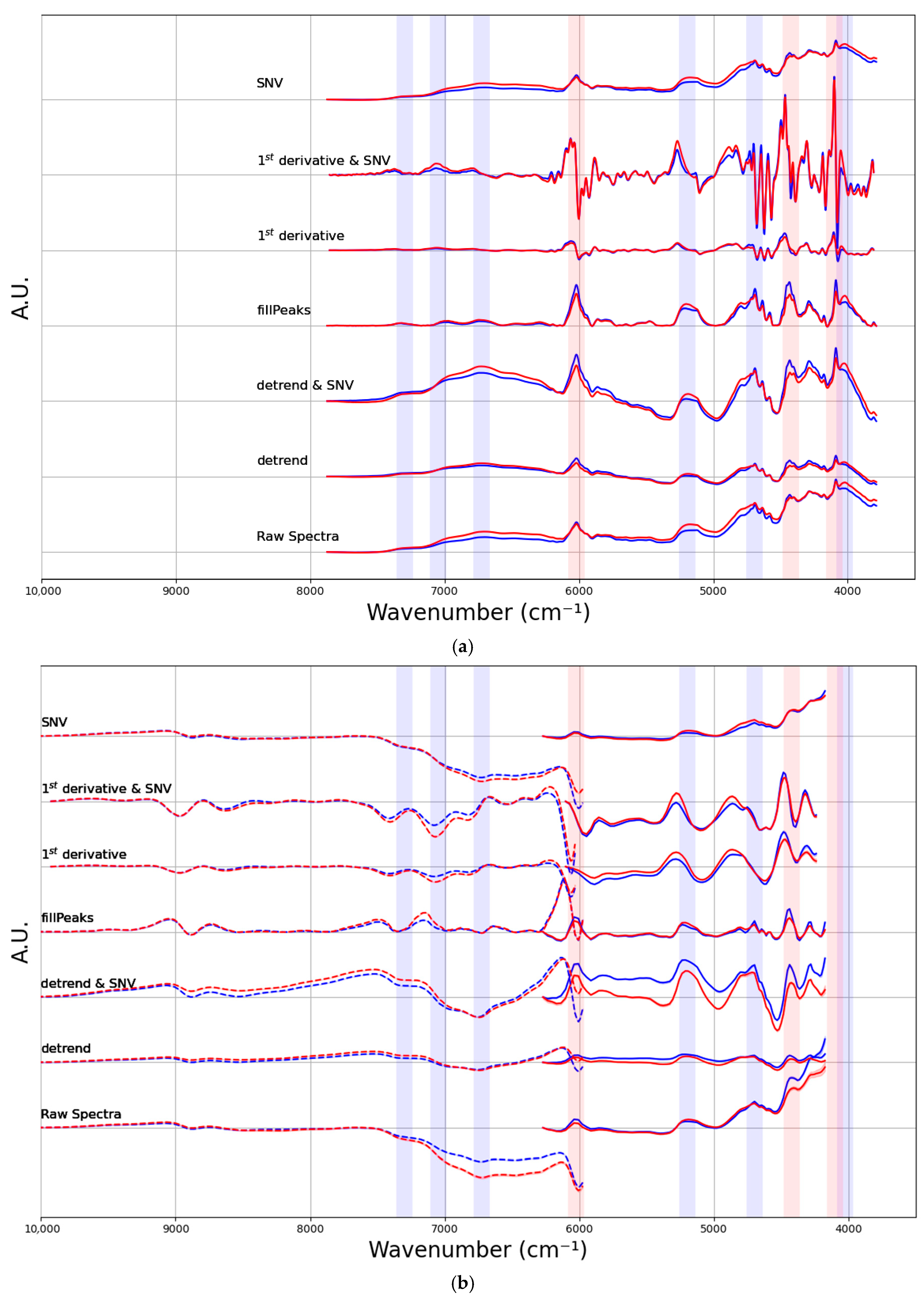
In Figure 1, the NIR spectra for benchtop NIR, handheld instrument, and imaging sensor system with and without preprocessing are shown. The spectra from the handheld instrument and the imaging sensor system exhibit a reduced level of structure regarding the number of bands, a consequence of the lower resolution (Table 1) and overall performance of these instruments. This effect is particularly evident in the imaging sensor system. Its design focuses on robustness and high-throughput industrial applicability rather than detailed chemical resolution, which inherently limits the number of exploitable spectral features and results in a pronounced reduction in spectral detail. The comparatively lower spectral resolution leads to increased band overlap and a reduced ability to resolve weak overtone and combination bands. Therefore, chemical specific information is concentrated in broad absorption regions rather than in distinct spectral features, making these systems more dependent on robust preprocessing strategies.

Consequently, the applied preprocessing methods markedly influenced the spectral appearance (Figure 1). In particular, the fillPeaks approach reduced low-frequency intensity variations and enhanced the visual prominence of absorption features. Application of the Savitzky–Golay first-derivative transformation resulted in visibly smoother spectral profiles with reduced high-frequency fluctuations, particularly for the handheld and imaging sensor system. This indicates effective attenuation of noise while maintaining the overall band structure [47]. Beyond the use of the first derivative alone, a combined preprocessing strategy was also evaluated, as suggested by Stipanovic et al. [33]. Using the combination of the first derivative and SNV increased the intensity of the resulting signals, revealing more pronounced differences between spectra with low and high cotton content.

This observation is illustrated by the bands near 4000 cm⁻¹ and 5200–5300 cm⁻¹ (Figure 1a). In addition, the combination of detrending with SNV appears to be a more promising approach, as evidenced by the observation of distinct differences when compared with the use of detrending or SNV alone. The beneficial effect of SNV- and detrend-based preprocessing might be attributed to the correction of multiplicative scatter effects caused by textile surface roughness, fiber orientation, and path length variations, which are particularly pronounced in fibrous materials.

Characteristic absorption bands for cotton and polyester were assigned based on reported vibrational modes and their corresponding overtone or combination bands in the literature [14,22,33,48] (indicated by vertical bars in Figure 1). Weak bands at around 7300 cm⁻¹ (combination bands of C-H vibrations) [33,48] and 7050 cm⁻¹ (first overtone of O-H stretching modes) [33,48] can be seen. A prominent feature of cotton is the band around 6700 cm⁻¹ that is referenced in literature as first overtone O-H/C-H [22] with respect to combined O-H stretching and bending vibrations [14].

The intense band around 5200 cm⁻¹, assigned to O–H-related overtone and combination modes with respect to overtone of C=O [22,48], showed a clear dependence on cotton content [33]. Additionally, the band at approximately 4700 cm⁻¹ (attributed to a combination overtone of C–C/C–H and O–H [22] or to combined O–H stretching and bending vibrations [14]), and the band at around 4000 cm⁻¹ (combination of O-H and C-O stretching vibrations [48]) also appear to be related to the cotton content [33]. Although several of the discussed absorption bands are associated with O–H vibrations, variations in moisture content can be excluded as a confounding factor, as all samples were conditioned for at least 24 h at ambient temperature and measured within a narrow and controlled time window. Therefore, the observed spectral differences can be attributed primarily to cellulose-related vibrational modes rather than to fluctuations in sample moisture.

In the case of polyester, characteristic absorptions include a band near 6025 cm⁻¹, which reflects the first overtone of aliphatic and aromatic C–H vibrations [22,33]. Additionally, the region around 4425 cm⁻¹ is associated with combination bands involving C–C, C–H, and C=O vibrations [22]. A further band appears at around 4100 cm⁻¹, although no specific assignment was found in the referenced literature.

These spectral characteristics are primarily governed by instrument-specific properties such as spectral resolution and the signal-to-noise ratio, while preprocessing modifies their representation to a lesser extent. They provide the basis for comparing regression models and interpreting differences in predictive performance across the NIR systems investigated.

3.2. Performance Comparison of Regression Models Under Different Preprocessing Conditions

The Savitzky–Golay approach combines local polynomial smoothing with derivative calculation, enabling a reduction in high-frequency noise components when an appropriate window size is selected. As reported in the literature, (excessively) large Savitzky–Golay first-derivative window sizes may lead to oversmoothing and loss of relevant spectral features, whereas very small window sizes can result in insufficient smoothing and increased noise amplification [47,49]. Therefore, the influence of different window sizes on model performance was evaluated (Supplementary Materials, Tables S2–S4).

For partial least squares (PLS) regression, the lowest RMSEP values for both the handheld NIR instrument and the imaging sensor system were obtained using a window size of 11 (handheld: RMSEP = 1.70%; imaging sensor system: RMSEP = 1.15%). For the benchtop NIR system, a window size of 21 yielded the lowest RMSEP (1.12%), closely followed by a window size of 11 (1.16%). A similar trend was observed for the coefficient of determination, with the highest R² values achieved at a window size of 11 for the imaging sensor system (R² = 0.92) and the handheld instrument (R² = 0.81), while the benchtop system reached its highest R² at a window size of 21 (R² = 0.92). For the kernel-based LS-SVM model, the lowest RMSEP values were consistently obtained using a window size of 11 across all instruments (imaging sensor system: RMSEP = 1.16%; handheld: RMSEP = 1.69%; benchtop: RMSEP = 1.13%). The corresponding R² values showed slightly more variation, with the best results achieved at a window size of 5 for the imaging sensor system, 11 for the handheld instrument, and 21 for the benchtop system. However, particularly for the benchtop instrument, the differences between window sizes 11 and 21 were marginal. For the tree-based Random Forest model, the best performance in terms of both RMSEP and R² was obtained at a window size of 11 for the imaging sensor system, while a window size of 5 performed best for the handheld instrument. For the benchtop system, similar results were observed for window sizes of 11 and 21, with a slight advantage for the larger window. Overall, these results demonstrate that the choice of the Savitzky–Golay window size is a relevant preprocessing parameter that depends not only on the regression method but also on the spectral resolution and characteristic bandwidths of the respective instrument. To ensure comparability across models and instruments, a window size of 11 was selected for subsequent analyses and visualizations, including the heatmap representation and the combination of the first derivative with SNV normalization, as previously suggested by Stipanovic et al. [33].

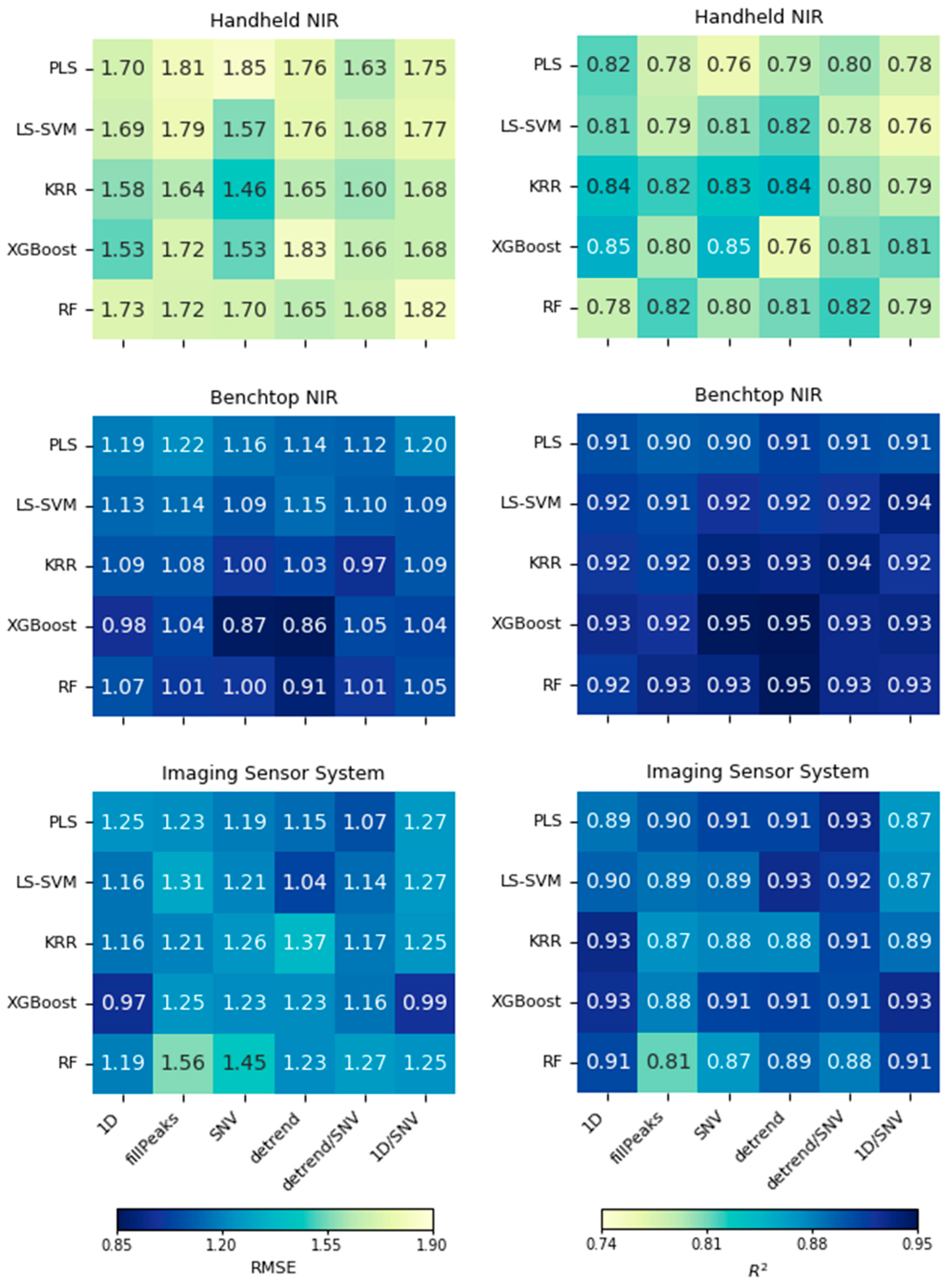
Following the selection of the appropriate Savitzky–Golay first-derivative window size of 11, the influence of different preprocessing strategies on model performance was systematically evaluated (Figure 2). For PLS regression, the best RMSEP values for the handheld and benchtop NIR instruments were obtained using a combination of detrending and SNV (handheld: RMSEP = 1.62%; benchtop: RMSEP = 1.08%), whereas for the imaging sensor system, the first derivative resulted in the lowest RMSEP (1.15%). R² values for the benchtop instrument were largely independent of preprocessing, ranging between 0.91% and 0.92%. For the handheld instrument, the highest R² was achieved using the first derivative combined with SNV (0.82), followed by detrending (0.81), while detrend/SNV ranked fourth (0.80). For the imaging sensor system, the first derivative also yielded the highest R² (0.92). The relative drop in R² between the best and worst preprocessing methods was moderate (approximately 7.5% for the imaging sensor system and handheld, and 3.5% for the benchtop system), whereas RMSEP was much more sensitive, with performance deteriorations exceeding 35%, nearly 20%, and more than 10%, respectively.

For LS-SVM, the optimal preprocessing method depends on the instrument. The lowest RMSEP values were obtained using detrending for the imaging sensor system (RMSEP = 1.04%) and SNV for the handheld (1.57%) with respect to the benchtop instruments (1.09). R² rankings showed greater variability, with detrending yielding the highest values for the imaging sensor system and handheld instrument, while the first derivative combined with SNV performed best for the benchtop system. The drop from the best to the worst preprocessing method amounted to nearly 20% in RMSEP and over 5% in R² for the imaging sensor system, around 13% RMSEP and 7% R² for the handheld instrument, and just over 5% RMSEP and 3% R² for the benchtop system.

After hyperparameter optimization (see below), Random Forest performance improved overall, but a strong dependence on preprocessing remained. For the imaging sensor system, the first derivative, evaluated across window sizes from 5 to 21, consistently yielded the lowest RMSEP values (1.06–1.19%) and the highest R² values (0.89–0.91). For the handheld instrument, several preprocessing strategies resulted in comparable RMSEP values (1.58–1.68%), while R² values remained low and similar (approximately 0.81). For the benchtop system, detrending achieved the lowest RMSEP (0.91) and the highest R² (0.95), closely followed by the first derivative.

For KRR and XGBoost, similar trends were observed, with the optimal preprocessing strategy being instrument dependent. For both models, differences in R² across preprocessing methods were generally smaller than those observed for RMSEP. For KRR, the lowest RMSEP values were obtained using detrend/SNV for the benchtop system, SNV for the handheld instrument, and the first derivative for the imaging sensor system, whereas fillPeaks and the combination of first derivative with SNV frequently resulted in elevated prediction errors. For XGBoost, the first derivative consistently achieved the lowest RMSEP for the handheld instrument and imaging sensor system, while detrending performed most favorably for the benchtop system. In both cases, fillPeaks was associated with the lowest predictive accuracy.

In summary, this data suggests that preprocessing is highly data-specific and should not be applied uniformly to all instruments or regression models. The benchtop NIR system, characterized by a high signal-to-noise ratio, exhibited comparatively stable performance across preprocessing methods, whereas handheld and imaging sensor systems showed substantially greater performance variability, indicating a higher sensitivity to preprocessing choices. Methods targeting scatter and baseline effects, such as detrending, SNV transformation, and first derivative-based preprocessing, were particularly important for the handheld instrument and the imaging sensor system. In contrast, fillPeaks exhibited strongly instrument-dependent behavior and frequently degraded performance for high-quality spectra by suppressing fine spectral structures. These findings emphasize that preprocessing decisions are especially critical for lower-resolution or noisier measurement systems, while their impact is reduced for high-quality benchtop instruments. Although the preprocessing strategy influenced performance within each instrument class, absolute differences between instrument types were substantially larger than differences introduced by preprocessing alone. This indicates that preprocessing acts primarily as a modulation factor within instrument-specific signal constraints rather than as an independent determinant of predictive accuracy.

3.3. Comparison of Regression Models and Preprocessing Strategies

Given the high dimensionality and strong multicollinearity of NIR spectroscopic data, overfitting represents a central challenge in model development. Therefore, model evaluation was not based only on absolute predictive performance (RMSEP, R²), but explicitly on the agreement between training and independent test data. In this context, RMSEC (training data set) and RMSEP (independent test prediction) were evaluated separately. All metrics, together with the corresponding R² values for training and test data, are reported to allow for assessment of model generalization and potential overfitting. In addition, model complexity measures (number of latent variables for PLS and selected hyperparameters for machine learning models) were documented to ensure a fair comparison between preprocessing strategies and regression approaches (Supplementary Materials). During initial model development, tree-based ensemble methods, particularly random forest and XGBoost, exhibited near-perfect fits on the training data for several preprocessing strategies (RMSEC random forest first derivative with SNV benchtop and imaging sensor system <0.05%). This behavior necessitated a more restrictive and carefully controlled hyperparameter optimization to reduce model variance and improve generalization. Therefore, random forest hyperparameters were regularized by limiting tree depth, increasing minimum split and leaf sizes, and enabling bootstrap aggregation (Supplementary Materials, Table S1), which substantially reduced overfitting and improved the consistency between training and test performance. The other regression models were also trained using model-intrinsic regularization or restricted hyperparameter settings (Supplementary Materials, Table S1) that corresponded to their respective learning principles. This approach made it possible to focus on model comparisons on generalization behavior rather than on differences resulting from the unrestricted flexibility of the models.

Against this background, PLS regression was used as a linear reference model to provide a robust reference for predictive performance across the different instruments. The optimal number of latent variables varied depending on preprocessing strategy and instrument class and is reported in the GitHub repository. Overall, PLS exhibited stable but comparatively limited predictive performance. For the benchtop NIR system, detrending and detrending combined with SNV preprocessing yielded the best results, with RMSEP values around 1.08–1.11% and R² values of approximately 0.90–0.92. In contrast, the handheld instrument exhibited substantially higher RMSEP values (approximately 1.62) and greater variability in R², reflecting the reduced spectral resolution and increased noise level of this system. For the imaging sensor system, first-derivative preprocessing resulted in the best PLS performance (RMSEP 1.15%; R² 0.92), indicating that preprocessing and enhancement in broad spectral trends are particularly important for low-resolution measurements.

LS-SVM models provided improved performance compared to PLS by enabling non-linear regression within a regularized framework. Model performance was strongly dependent on preprocessing strategy, with SNV-based approaches generally yielding the most favorable results. For the benchtop instrument, LS-SVM achieved performance comparable to PLS, whereas for the handheld instrument and the imaging sensor system, clear improvements in RMSEP and R² were observed. Hyperparameter optimization revealed instrument-dependent regularization requirements, with lower regularization parameters favored for the benchtop system and higher values required for the noisier handheld and imaging sensor system data. These results indicate that LS-SVM can adapt to varying data quality while maintaining stable generalization behavior.

Kernel ridge regression consistently delivered strong generalization performance. Benefiting from its explicit L2 regularization, KRR effectively controlled model complexity in the presence of strong multicollinearity. For the benchtop NIR system, the combination of detrending and SNV preprocessing with KRR resulted in the lowest RMSEP values among all evaluated models, representing a substantial improvement of 10% compared to PLS regression. Similar, though less pronounced, improvements were observed for the handheld instrument. In contrast, first-derivative preprocessing frequently degrades KRR performance, emphasizing the importance of aligning preprocessing strategies with model characteristics. Optimal regularization parameters [50,51] were consistently found in the low-to-moderate range (α ≈ 0.01–0.05), corresponding to minima in validation error and indicating a favorable bias–variance trade-off.

Although XGBoost demonstrated high predictive potential, exemplified by an improvement of up to 9% for the handheld instrument compared to PLS regression, it exhibited a pronounced tendency towards overfitting, particularly for the benchtop and imaging sensor system. Even when the hyperparameter space was constrained to flat or moderately deep trees, reduced learning rates, and subsampling, substantial discrepancies between training and test performance were frequently observed. This behavior can be attributed to the sequential nature of gradient boosting, whereby residuals are iteratively corrected following the framework introduced by Friedman [52], which can amplify noise and instrument-specific artefacts in high-dimensional and strongly correlated spectral data. Hyperparameter optimization consistently favored strongly regularized configurations with shallow trees and subsampling; nevertheless, predictive performance remained unstable, particularly for the imaging sensor system, highlighting the high sensitivity of boosting methods to data quality and sample size. This behavior is consistent with previous benchmarking studies reporting high tunability but limited robustness of boosting models compared to random forests [53]. Future work could further improve model robustness by extending the hyperparameter space to include explicit regularization terms such as minimum child weight, split loss thresholds (gamma), and L1/L2 penalties, as well as by applying early stopping strategies based on independent validation sets or nested cross-validation.

The random forest regression model demonstrated strong and comparatively stable predictive performance across all instruments, with RMSEP values ranging from approximately 0.91–1.19% for the benchtop system, and with moderate performance for the imaging sensor system (RMSEP ≈ 1.19%, R² ≈ 0.91). The handheld instrument exhibited slightly higher errors, with RMSEP values ranging from 1.65–1.68%, and with R² values ranging from 0.81 to 0.82. By constraining tree depth, enforcing conservative node splitting criteria, and enabling bootstrap aggregation, model variance was effectively controlled, resulting in improved agreement between training and test performance. Inspection of the optimized random forest hyperparameters revealed a high degree of consistency across instruments. Optimal configurations were characterized by moderate tree depths (max_depth = 10–20), conservative splitting criteria, and standard feature subsampling strategies (√ or log2), indicating that performance gains were achieved without excessive model complexity, consistent with the inherent variance-reducing design of random forests [54]. Notably, the optimization procedure consistently selected the lowest allowed value for the minimum number of samples per leaf (min_samples_leaf = 5) across instruments, indicating a tendency of the model to favor highly flexible tree structures. Due to the rapidly increasing computational cost associated with larger hyperparameter spaces, the range of evaluated random forest configurations had to be deliberately constrained. The discussed observations are consistent with the findings of previous large-scale benchmark studies, which have reported comparatively low tunability of random forest models and a tendency towards robust, near-default configurations [50,53].

Summarized for the benchtop NIR system, advanced regression models consistently achieved high predictive accuracy, with RMSEP values around or below 1.00% and R² values of approximately 0.94–0.95 for RF, XGBoost, LS-SVM, and KRR. These results clearly outperform standard PLS regression, which yielded an RMSEP of 1.08% and an R² of 0.91. The high signal-to-noise ratio and spectral resolution of the benchtop instrument enabled robust exploitation of nonlinear relationships, particularly when combined with appropriate preprocessing.

For the handheld NIR instrument, model performance was more heterogeneous and less consistent. Although advanced models generally outperformed PLS regression, prediction errors were higher overall. RMSEP values between 1.46 and 1.56% with corresponding R² values of 0.81–0.85 were observed, compared to PLS regression with an RMSEP of 1.62% and an R² of 0.80. Notably, random forest did not consistently outperform PLS for the handheld system, indicating that increased model complexity does not necessarily translate into improved performance for lower-resolution or noisier instruments. For the imaging sensor system, gradient boosting models frequently exhibited unstable behavior and pronounced overfitting. The best XGBoost results reached an RMSEP of approximately 1.25% with an R² of 0.88, whereas the remaining regression models achieved substantially more robust performance, with RMSEP values between 1.03 and 1.13% and R² values of 0.90–0.93. These results are comparable to or slightly better than those obtained with PLS regression (RMSEP = 1.15%, R² = 0.92) and exceed the predictive performance observed for the handheld instrument, despite the lower spectral resolution of the imaging sensor system.

Across all instruments, no single regression model or preprocessing strategy was universally optimal. In line with the No Free Lunch Theorem [41], model performance was strongly context-dependent and governed by instrument-specific characteristics such as spectral resolution, noise level, wavelength coverage, and the interaction between preprocessing and model-intrinsic regularization. The comparison further demonstrates that preprocessing strategies not only affected predictive accuracy but also influenced model complexity, reflected in varying numbers of latent variables for PLS and instrument-dependent hyperparameter configurations for nonlinear models. Under more heterogeneous real-world conditions, these interactions are expected to become even more pronounced. Increased surface roughness, dyeing, and structural variability would likely enhance the relevance of scatter-correction methods such as SNV or MSC, while derivative-based preprocessing may help suppress broad background contributions but simultaneously amplify noise in lower-resolution inline systems. Spectral regions dominated by cellulose-specific O–H combination bands may remain comparatively robust, whereas weaker overtone regions could lose discriminative power due to overlapping contributions from colorants and additives.

3.4. Model Interpretability: Coefficients and Feature Relevance

Feature importance analysis was performed for XGBoost and partial least squares (PLS) regression, as both provide interpretable measures of variable relevance. In XGBoost, importance is derived from variable contributions to tree splits [55], while PLS relates spectral variables to latent components maximizing covariance with the response, allowing for physically meaningful interpretation [34,56].

XGBoost Model Interpretability

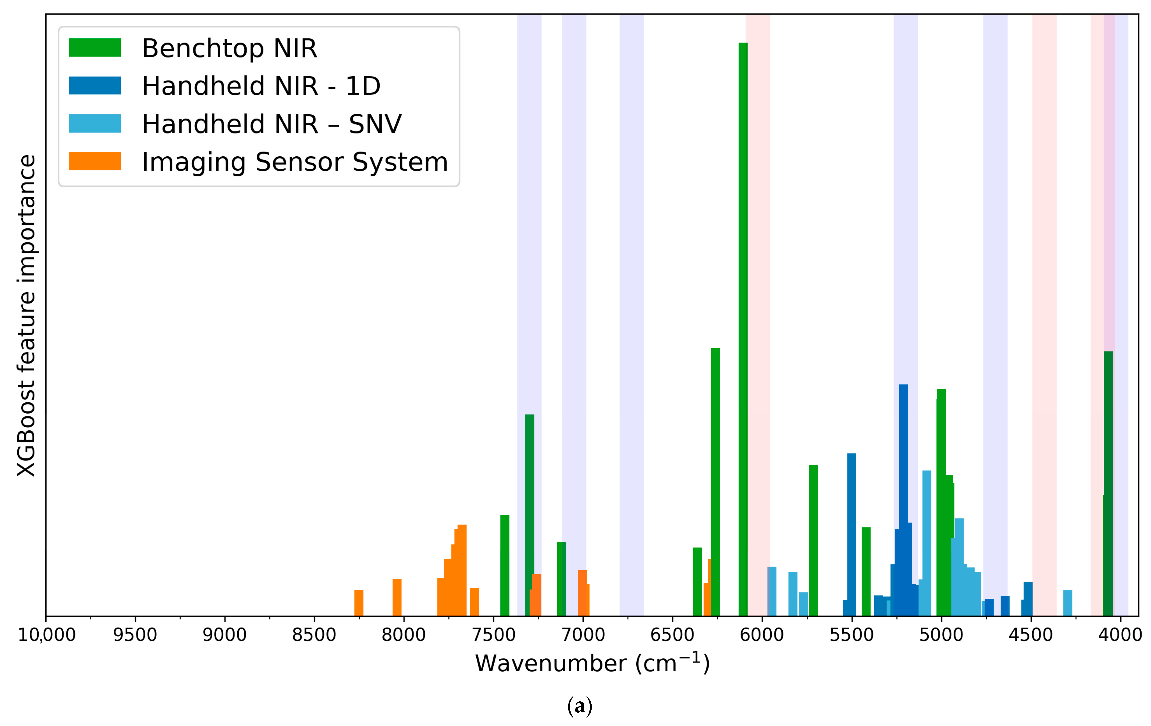
The XGBoost feature importance analysis (Figure 3a) was performed separately for the imaging sensor system, the handheld device, and the benchtop system. For each instrument, the preprocessing strategy yielding the most robust generalization performance was selected (imaging sensor system: fillPeaks; handheld: first derivative resp. SNV; benchtop: detrend + SNV). The interpretation therefore focuses on system-specific, model-relevant features rather than on preprocessing-independent trends.

For the imaging sensor system, the most important XGBoost features are predominantly located in the region between approximately 7600 and 7700 cm⁻¹, with additional contributions above 7000 cm⁻¹. These wavenumbers dominate the model decision and reflect the limited spectral resolution and overall performance of the imaging sensor system, which favors statistically stable overtone regions over well-resolved band structures. Among the identified features, a contribution around 7300 cm⁻¹, attributed to combination bands of C–H vibrations, overlaps with a literature-reported cotton-related absorption. Other characteristic cotton bands, such as those around 6730 or 5200 cm⁻¹, are not relevant for this system and do not appear in the feature importance ranking. Polyester-related features are likewise not dominant in the imaging sensor system data.

For the handheld instrument, XGBoost feature importance was evaluated using the two best preprocessing strategies, first derivative and SNV, both of which yielded comparable predictive performance. A direct comparison of the feature rankings obtained with these two preprocessing approaches reveals a high degree of consistency in the spectral regions exploited by the model. In both cases, the most important features cluster around the cotton-related bands near 5200 cm⁻¹ and 4700 cm⁻¹. Although the exact numerical positions and ranking order of individual wavenumbers differ between first derivative and SNV preprocessing, these differences represent small shifts within broad near-infrared bands. In contrast, polyester-related absorptions around 4400 cm⁻¹, which are clearly visible in the preprocessed NIR spectra (Figure 1), do not appear among the most important XGBoost features. This observation indicates that, while these bands are spectrally present, they do not contribute significantly to the statistical separation achieved by the model. Instead, the XGBoost classifier primarily relies on cotton-associated spectral regions. This behavior reflects both the limited spectral resolution of the handheld instrument and the tendency of tree-based models to select the most statistically robust spectral regions rather than all spectroscopically observable features.

For the benchtop system, which achieved the highest predictive performance, the most important XGBoost features are concentrated at discrete wavenumbers, most notably around 6260 cm⁻¹, with additional relevant contributions in the regions around 5000 cm⁻¹ and 4000 cm⁻¹. The high signal-to-noise ratio and spectral resolution of the benchtop system enable the model to rely on a small number of robust and reproducible spectral features. With respect to material-specific bands, only a limited subset of previously assigned absorptions contributes to the model decision. Cotton-related features are observed at ~7300 cm⁻¹ and ~4069 cm⁻¹, whereas other literature-reported cotton bands (e.g., around 7050, 6730, 5200, or 4700 cm⁻¹) do not appear among the most important XGBoost features. For polyester, contributions at around 4100 cm⁻¹ and 6025 cm⁻¹ appear in the features, while other polyester-related bands are not relevant in the final model.

Across all systems, XGBoost selects point-wise spectral features that provide the highest statistical discrimination for the respective instrument and preprocessing strategy. While not all literature-reported cotton and polyester bands contribute equally to the models, several of the features coincide with known NIR overtone and combination bands. Therefore, the selected features should not be interpreted as isolated chemically specific signals but rather as representative points within spectrally relevant regions. In this context, PLS regression provides a more stable and physically interpretable representation of band structures.

PLS Model Interpretability

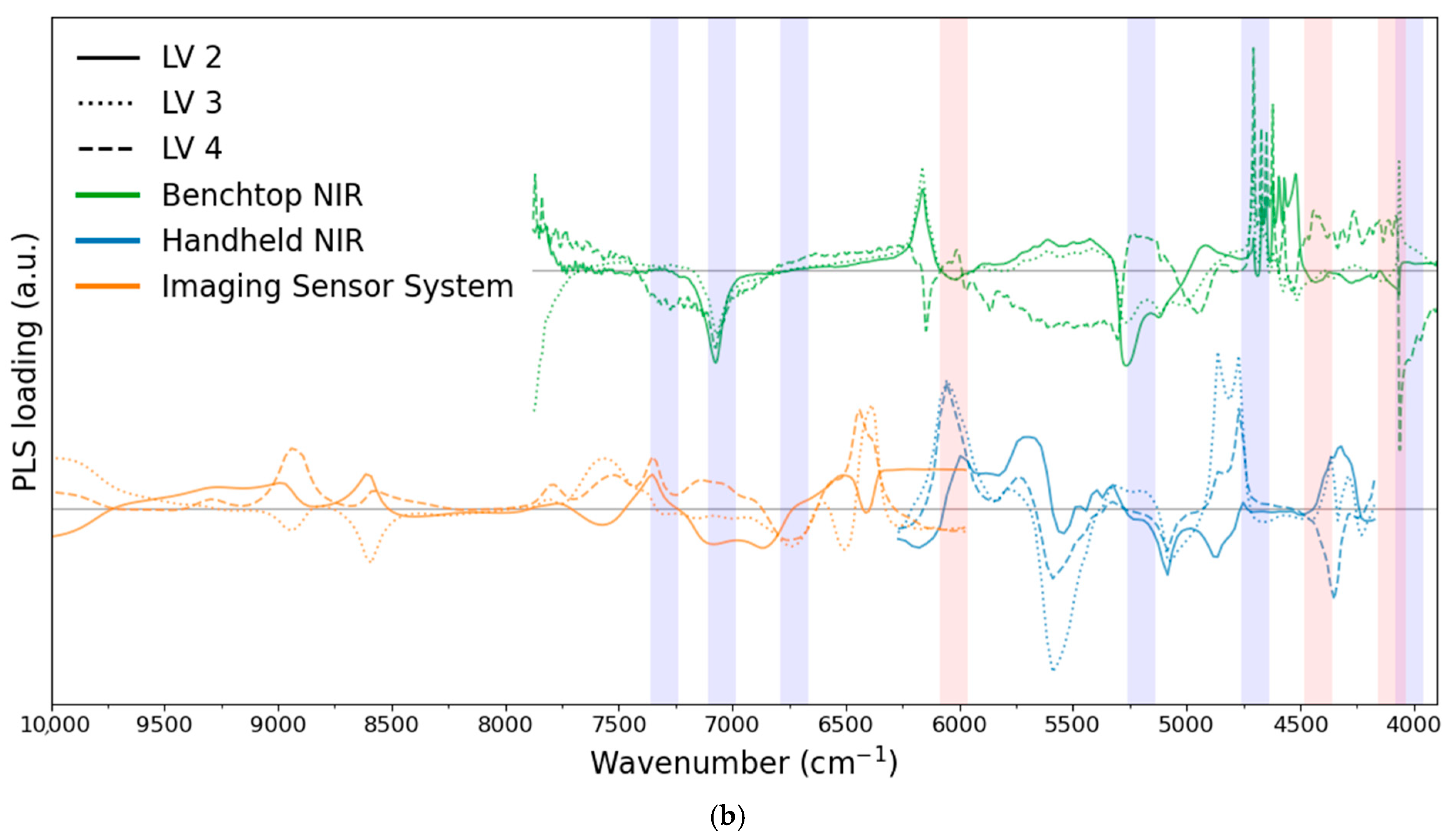
For PLS regression, latent variables 2–4 were interpreted, as the first latent variable mainly captured dominant, globally correlated spectral variance rather than material-discriminative chemical information.

For the imaging sensor system, PLS loadings of components 2–4 are broad and weak, reflecting the limited spectral resolution and restricted wavelength coverage of the system (Figure 3b). Alternating positive and negative loadings appear around 9000–8800 cm⁻¹ and near 8600 cm⁻¹, but these features cannot be unambiguously linked to specific molecular vibrations. The interval between 8400 and 8000 cm⁻¹ is largely featureless, with only weak contributions near 7800 cm⁻¹ and slightly more pronounced but unspecific features around 7600 cm⁻¹. Chemically more meaningful contributions emerge at lower wavenumbers. Positive loadings for components 2 and 4 are observed around 7300 and 6700 cm⁻¹, coinciding with literature-reported cotton-related overtone and combination bands. A feature near 6400 cm⁻¹ does not correspond to known cotton or polyester absorptions and is interpreted as non-specific variance.

For the handheld NIR system, PLS loadings of components 2–4 exhibit more pronounced and structured features. Positive loadings around 6000 cm⁻¹ can be associated with polyester-related bands, indicating that the handheld instrument captures material-specific information from both fiber components. Strong negative loadings occur around 5600 cm⁻¹, although no clear cotton or polyester assignment could be identified, suggesting overlapping combination bands or systematic spectral variance. Negative loadings near 5100 cm⁻¹ are observed close to the well-established cotton-related band at around 5200 cm⁻¹, indicating contributions from cotton-associated bands. Additional positive and negative loadings below 4400 cm⁻¹ overlap with cotton-related absorptions in the 4400–4500 cm⁻¹ region. Particularly intense features for components 2 and 3 are found between 4800 and 4900 cm⁻¹, a region frequently associated with cotton-dependent combination bands. Overall, both cotton- and polyester-related regions contribute to the latent variables, although several strong features remain difficult to assign unambiguously.

The benchtop NIR system shows the most distinct and chemically interpretable PLS loadings, consistent with its superior spectral resolution, broader wavelength range, and highest predictive performance. Negative loadings for components 2–4 are observed around 7000–7100 cm⁻¹, coinciding with cotton-related overtone bands. Strong positive and negative loadings occur between 6200 and 6100 cm⁻¹, associated with polyester-related overtones, as well as near 5200–5300 cm⁻¹, corresponding to prominent cotton-related bands. Additional intense features are present around 4700 cm⁻¹, which are well-known to be sensitive to cotton content, while smaller features near 4400 cm⁻¹ coincide with polyester-related absorptions. Below 4200 cm⁻¹, several features of varying intensity overlap with both cotton- and polyester-related bands, highlighting the ability of the benchtop system to capture chemically meaningful variance across multiple relevant spectral regions.

Across all instruments, cotton-related spectral regions contribute to the latent variables used for prediction; however, their number, clarity, and interpretability strongly depend on the instrument class. The imaging sensor system captures only a small subset of cotton-associated bands, the handheld system reflects contributions from both cotton and polyester with several ambiguous features, and the benchtop NIR system exhibits the most comprehensive and chemically interpretable loading structure. The clearer chemical interpretability observed for the benchtop system further supports the conclusion that instrument-dependent signal quality, rather than preprocessing alone, governs the robustness of spectroscopic modeling.

While XGBoost identifies point-wise spectral positions that maximize statistical discrimination within non-linear decision rules, PLS loadings represent distributed spectral patterns across broader absorption regions. An alternative to interpreting individual loadings would be the calculation of variable importance in projection (VIP) scores [57], which provide a concise summary of the overall relevance of each variable. However, in the present study, loadings were intentionally examined to preserve the structure of the latent variables. As XGBoost feature importance is driven by statistical contributions to model decisions, spectral interpretation was mainly guided by PLS regression, which provides physically meaningful loadings linked to spectral covariance with the response variable. More advanced model-agnostic interpretability approaches such as SHAP (SHapley Additive exPlanations) values [58] may provide additional insights into non-linear model behavior, but these were beyond the scope of the present study.

3.5. Model Training Time

The influence of spectral pre-treatment on training time varied substantially across models and instruments (Supplementary Materials, Tables S2–S4). It should be noted that the reported training times also depend on the hyperparameter optimization budget, i.e., the size of the search grid. Consequently, absolute runtimes are not solely a property of the learning algorithm and preprocessing, but scale approximately with the number of evaluated parameter combinations. For PLS regression, preprocessing had only a minor effect on computational cost. Neither detrending, SNV, nor different Savitzky–Golay window sizes altered training time meaningfully for the handheld or imaging sensor system instruments. The benchtop system exhibited a slightly higher variability (coefficient of variation: 15.9%), yet, even here, the differences between pre-treatments remained moderate. Among the pre-treatments, fillPeaks resulted in the longest PLS training times, whereas window-size effects of Savitzky–Golay filters remained negligible. Across instruments, the handheld NIR exhibited 1.37-fold longer PLS training times than the imaging sensor system, whereas the benchtop instrument required 351-fold longer training times. The generally higher training times for benchtop PLS models are primarily attributable to the substantially higher spectral resolution, which increases matrix dimensionality and thereby amplifies the scaling behavior of PLS. This reflects the dominant role of spectral dimensionality rather than the chosen pre-treatment. KRR displayed a highly consistent computational profile across pre-treatments, as indicated by low coefficients of variation (handheld: 4.93%, imaging sensor system: 6.75%, benchtop: 7.39%). Relative to the handheld instrument, the imaging sensor system was approximately 2.4 times faster, whereas benchtop data resulted in a 2.6 times slower training process. A similar pattern was observed for LS-SVM. Here, pre-treatments again had negligible influence, including the Savitzky–Golay window size. The variability remained low to moderate across instruments (handheld: 6.69%, imaging sensor system: 17.7%, benchtop: 1.26%). Imaging sensor system data enabled the fastest training (4 times faster than handheld), whereas benchtop training times were modestly slower (1.7 times) than for handheld. Tree-based models showed the largest pre-treatment-related variability. For random forest, differences between window sizes and preprocessing strategies were more pronounced, reflected by substantially higher coefficients of variation (handheld: 31.1%, imaging sensor system: 30.9%, benchtop: 27.5%) compared to the other regression approaches. Despite this variability, the ranking of devices was consistent: the imaging sensor system enabled the fastest training (2.5 times faster than handheld), while benchtop spectra led to nearly tenfold higher training times. XGBoost displayed a similar behavior. Although differences between pre-treatments were visible (coefficient of variation: 13–16%), no systematic trend emerged. Again, the imaging sensor system produced the lowest training times (1.5 times faster than handheld), whereas benchtop spectra resulted in a nearly tenfold increase (9.5 times slower). Overall, the influence of preprocessing on training time was strongly model-dependent. For PLS and the kernel methods, pre-treatments introduced only minor runtime variation, indicating algorithmic robustness to spectral transformations. In contrast, tree-based ensembles were more sensitive to pre-treatment, likely due to their dependence on local variance structure and feature distributions. Savitzky–Golay filtering, especially with a window size of 21, often yielded the fastest runtimes across all instruments, although this pattern was not consistent.

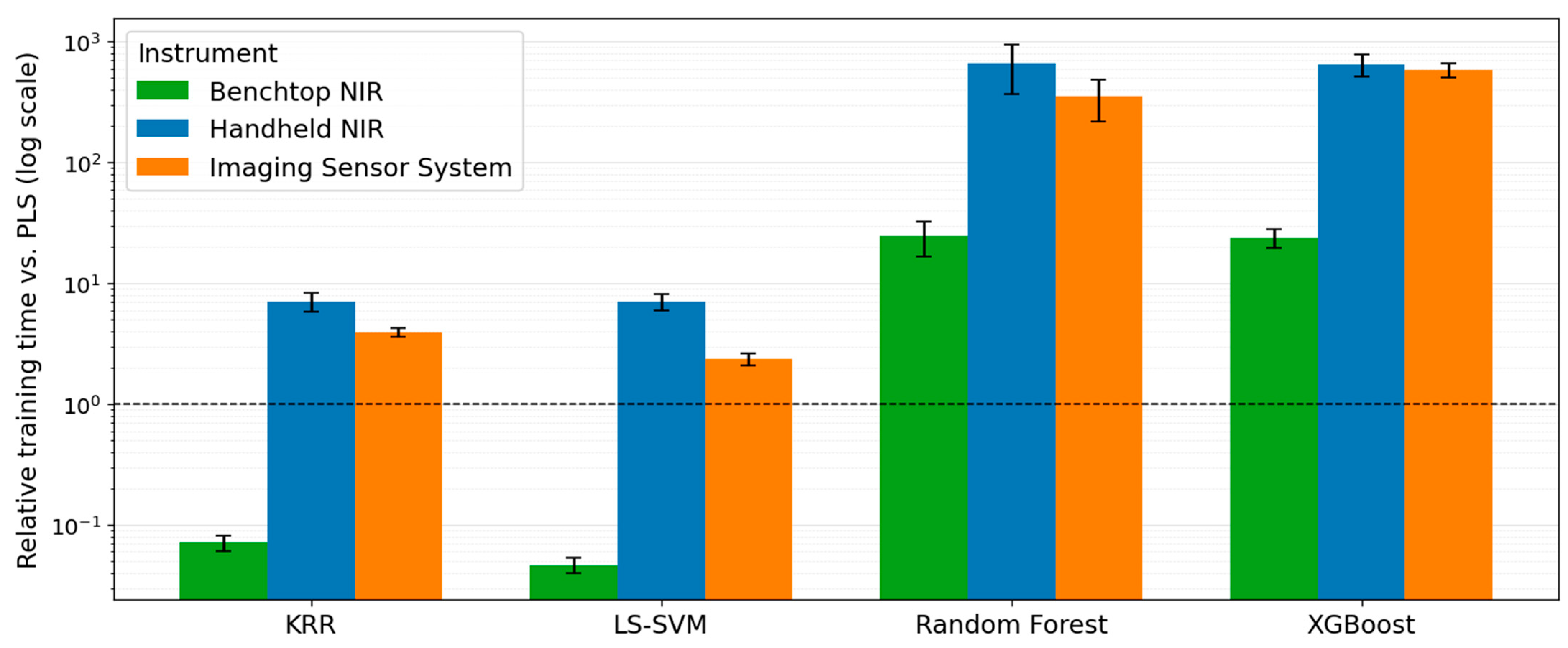
Building upon these pre-treatment-specific observations, the relative training times across models and instruments were compared to evaluate the overall computational behavior of the applied regression methods (Figure 4). PLS was used as the reference since this is the most common method in the literature. Across the handheld NIR and imaging sensor system, kernel-based methods (LS-SVM and KRR) require approximately one order of magnitude more training time than PLS, whereas ensemble models (random forest and XGBoost) exhibit increases of two to three orders of magnitude. These patterns reflect the higher algorithmic complexity of tree-based ensembles in high-dimensional spectral data, where repeated split evaluation and large model sizes dominate computation. The relatively small standard deviations for LS-SVM and KRR indicate stable computational behavior across preprocessing variants. By contrast, the greater variability observed for random forest is consistent with the sensitivity to preprocessing-induced changes. The computational costs for the handheld seem to be somewhat higher than with the imaging sensor system. In contrast, the benchtop dataset shows a different profile. Here, LS-SVM and KRR train substantially faster than PLS (ratios < 0.1), while the ensemble models remain more expensive but at markedly lower relative levels than for the other instruments. This is consistent with the previously mentioned explanation, as the higher spectral resolution increases the number of variables and thereby amplifies the computational cost of PLS regression.

Overall, the results demonstrate that PLS remains the most computationally efficient model across all instruments. Kernel methods result in moderate additional cost, but their efficiency can strongly depend on spectral quality and instrument characteristics. Tree-based ensemble models, as expected, are the most computationally intensive, particularly for lower-quality or more variable spectra. The reported computational costs refer exclusively to model training during method development and do not reflect real-time prediction, which is substantially faster once the model is deployed.

4. Conclusions

This study is based on a sample set of cotton/polyester textile fabrics of the same origin, but with different ratios of cotton/polyester. It provides a systematic evaluation of NIR spectroscopy across different instrument classes and analyzes their interaction with preprocessing strategies and regression models, with a particular focus on instrument-dependent performance. This work provides practical guidance on the selection of instrument-dependent preprocessing–model combinations that can be used in specific application scenarios.

The results clearly demonstrate that instrument class is the primary determinant of predictive performance. The benchtop NIR system consistently achieved the highest accuracy and robustness, benefiting from spectral resolution, broader wavelength coverage, and a higher signal-to-noise ratio. In contrast, the easy-to-handle and fast handheld instrument and the imaging sensor system exhibited increased sensitivity to preprocessing choices and model selection, highlighting intrinsic limitations imposed by reduced resolution and higher noise levels. These findings emphasize that data analysis strategies cannot be transferred between instrument classes without adaptation. Within instrument-specific signal constraints, spectral preprocessing influenced predictive performance to varying degrees. More pronounced effects were observed for lower-resolution and noisier measurement systems, while its impact remained comparatively moderate for the benchtop instrument. Methods addressing baseline distortions and scatter effects contributed to improved model stability for handheld and imaging sensor system data, while their effect was less pronounced for high-quality benchtop spectra.

Regarding the models used, PLS regression proves to be a robust and computationally efficient reference method, delivering stable but performance-limited results across all instruments. Nonlinear models are able to compensate for instrumental constraints to varying degrees. Kernel-based methods (LS-SVM and kernel ridge regression) consistently improve predictive accuracy while maintaining good generalization. Tree-based ensemble models achieve high performance in selected cases but exhibit a pronounced risk of overfitting and substantially higher computational costs. These observations underscore that increased model complexity does not automatically translate into better performance, particularly for noisy or low-resolution data. The analysis further showed that flexible nonlinear models were more susceptible to overfitting when applied to lower-quality spectral data, underscoring the importance of regularization and independent test validation when interpreting apparent performance gains.

These results offer valuable insights into the development of industrial textile recycling workflows under controlled conditions. For centralized laboratory-based tasks such as method development, calibration, and reference analysis, benchtop NIR systems combined with advanced regression models offer the highest accuracy and interpretability. In contrast, for automated inline textile sorting applications, the imaging sensor system represents the practically relevant solution, while handheld devices may support decentralized or assisted sorting scenarios. In these cases, carefully optimized preprocessing and moderately complex models are required to achieve reliable predictions within acceptable computational constraints.

Several limitations of the present study should be acknowledged. The dataset investigated covers a limited cotton content range, reflecting the conditions encountered during method development. Broader cotton/polyester ranges can be addressed and should be included in future model extensions. Moreover, the present work deliberately focused on ideal, white textiles and does not reflect the heterogeneity of real-world samples, such as aging or color effects. Aging and dyeing are expected to influence NIR spectra by introducing additional absorption features and altering scattering behavior, depending on the wavelength range used potentially affecting model performance and increasing calibration complexity [23,33]. The investigation of such effects, as well as potential influences on Raman spectra, was beyond the scope of this study [59]. Consequently, statements regarding robustness, transferability between instrument classes, and industrial applicability are restricted to the controlled sample system investigated here.

Future work will therefore focus on expanding the dataset with a wider variety of textile compositions, which is expected to improve model robustness and generalization to real-world textile waste streams. With increasing dataset sizes and objectives, and scalable outlier detection strategies, such as Mahalanobis distance or residual-based methods, it will become essential to replace manual filtering. Furthermore, automated feature and wavelength selection approaches [29,37,60] represent promising avenues to further enhance model performance, robustness, and interpretability.

In summary, this work demonstrates that reliable quantification of cotton content in blended textiles by NIR spectroscopy requires coordinated optimization of instrument choice, preprocessing strategy, and regression model. By explicitly accounting for instrument-specific constraints and computational considerations, the presented results provide a methodological framework that can support future validation studies aiming at industrial implementation under realistic textile conditions. Our results suggest that instrument characteristics determine the upper limits of performance, while model complexity governs generalization and preprocessing exerts a secondary, interaction-dependent influence.