Quantitative Assessment of Consistency Between IMO DCS and EU MRV Frameworks Using Large-Scale Operational Data

Abstract

This study presents a large-scale empirical comparison of operational efficiency metrics derived from the IMO Data Collection System (DCS) and the EU Monitoring, Reporting and Verification (MRV) framework. Paired non-parametric tests, effect size estimation, and agreement diagnostics were applied to a matched dataset of 15,755 dual-reported vessels and over 50,000 ship-year observations from 2019 to 2024 to assess consistency across monitoring systems. The results indicate that, although statistically significant differences are detected (p < 0.001), practical differences are negligible (Cohen’s d < 0.025), with MRV-based values averaging approximately 1.4% lower in Annual Efficiency Ratio (AER) and fuel intensity than DCS values. Distributional analysis confirms substantial overlap between the datasets, and temporal trends show progressive convergence following the implementation of the Carbon Intensity Indicator (CII) regulation. However, pronounced vessel-type heterogeneity is observed. Flexible cargo vessels exhibit consistent efficiency improvements in EU-related voyages, whereas container ships show minimal variation, and LNG carriers demonstrate indicator-dependent patterns. Overall, the findings indicate that the DCS and MRV frameworks provide broadly comparable representations of operational efficiency, with observed differences primarily reflecting vessel-type-specific operational characteristics rather than structural inconsistencies in the reporting systems. This study provides a scalable statistical validation framework for cross-regulatory monitoring assessment.

1. Introduction

International shipping serves as the backbone of global trade, transporting approximately 80% of world merchandise by volume. However, this essential sector contributes around 3% of global anthropogenic greenhouse gas (GHG) emissions, equivalent to over 1 billion tons of CO₂ annually [1]. As maritime decarbonization efforts intensify, large-scale monitoring systems have become essential tools for tracking operational efficiency and emission performance.

Two major data collection frameworks currently govern maritime GHG reporting: the IMO Data Collection System (DCS) and the EU Monitoring, Reporting and Verification (MRV) system. The IMO DCS, operational since 2019, requires ships above 5000 gross tonnage engaged in international voyages to report annual fuel consumption, distance traveled, and hours underway [2]. The EU Monitoring, Reporting and Verification (MRV) Regulation, in force since 2018, mandates ships calling at EU ports to report CO₂ emissions, fuel consumption, and transport work for voyages involving EU ports, with voyage-level granularity and public data availability [3,4].

While both systems share the common objective of enhancing transparency in maritime emissions, they differ in geographic scope, reporting granularity, and transparency. Such structural differences introduce potential discrepancies in efficiency indicators derived from the two datasets. Ensuring cross-platform consistency is, therefore, critical to reliable performance assessment, indicator calibration, and monitoring-system validation.

Recent regulatory developments further increase reliance on large-scale operational datasets for performance evaluation. The IMO adopted its revised GHG Strategy in 2023, setting a net-zero target by or around 2050 with intermediate checkpoints [5]. The Carbon Intensity Indicator (CII) regulation, effective from 2023, converts DCS-reported fuel consumption and activity data into operational efficiency ratings [6,7]. Concurrently, the EU has implemented FuelEU Maritime [8] and extended the EU Emissions Trading System (EU ETS) to maritime transport [9], both of which utilize MRV-reported emissions and activity data as quantitative compliance inputs. As these regulatory instruments increasingly depend on reported operational datasets, rigorous assessment of cross-system data consistency becomes critical to reliable performance evaluation and monitoring-system validation.

Despite the critical importance of data consistency for regulatory harmonization, no comprehensive statistical comparison of efficiency metrics derived from matched DCS-MRV observations has been published in the peer-reviewed literature. Existing studies have primarily focused on institutional comparisons [4] or single-dataset analyses [10,11], without systematically quantifying vessel-level discrepancies using paired statistical methodologies.

This study addresses this gap by developing and applying a reproducible statistical validation framework to matched operational datasets from 15,755 dual-reported vessels over six years (2019–2024), comprising more than 50,000 ship-year observations. The analysis integrates paired non-parametric testing, effect size estimation, and agreement diagnostics to evaluate discrepancies in key efficiency indicators. Temporal convergence patterns following the implementation of the Carbon Intensity Indicator (CII) regulation are also examined to assess whether global operational behavior has become increasingly aligned across regulatory regimes.

By establishing a scalable quantitative approach for cross-platform monitoring-system validation, this study contributes to applied maritime data analytics and provides methodological tools for evaluating large regulatory datasets.

Moreover, we make three primary contributions to the literature on maritime emission monitoring and regulatory data analysis.

First, we construct the first large-scale matched dataset linking ship-level observations from the IMO Data Collection System (DCS) and the EU Monitoring, Reporting and Verification (MRV) framework. The resulting dataset includes 15,755 dual-reported vessels and more than 50,000 ship-year observations spanning 2019–2024, enabling systematic cross-system comparison at an unprecedented scale.

Second, this study provides the first empirical validation of operational efficiency consistency between global (DCS) and regional (MRV) monitoring frameworks using paired statistical diagnostics, including non-parametric testing, effect size estimation, and Bland–Altman agreement analysis.

Third, in this analysis, we identify vessel-type-specific operational heterogeneity underlying observed discrepancies between the two monitoring systems, highlighting the role of operational flexibility, routing characteristics, and technical constraints in shaping efficiency differences across maritime segments.

The remainder of this paper is organized as follows: In Section 2, we review the related literature on monitoring-system comparisons, and in Section 3, we outline the regulatory data structures. In Section 4, we describe the research methodology and statistical framework, and in Section 5, we present the empirical results. A discussion on methodological implications for monitoring-system evaluation is provided in Section 6, and conclusions are given in Section 7.

2. Literature Review

2.1. Structural Characteristics of DCS and MRV Data Reporting Systems

The parallel implementation of the IMO Data Collection System (DCS) and the EU Monitoring, Reporting and Verification (MRV) framework has attracted scholarly attention regarding their structural design and reporting characteristics. These studies primarily examine differences in data granularity, transparency, and reporting architecture rather than conducting quantitative validation of reported operational metrics.

Adamowicz [4] conducted a comprehensive analysis of the coexistence of the EU MRV Regulation and the IMO DCS, examining enforcement mechanisms, port state control implications, and penalty structures. The study highlighted that while both systems target ships above 5000 GT, they differ fundamentally in data transparency—the EU MRV Regulation mandates public disclosure of individual ship data through the THETIS-MRV platform, whereas IMO DCS data remain confidential at the ship level. They concluded their analysis noting that regulatory alignment would require addressing these structural differences but did not provide a quantitative comparison of reported data.

Zis and Psaraftis [11] examined operational measures to mitigate potential modal shifts resulting from environmental legislation in the maritime sector. While their study focused primarily on the competitive implications of sulfur regulations for short-sea shipping, it established important methodological precedents for analyzing how regulatory changes affect fleet operational behavior—a framework subsequently applied to MRV-related research.

Psaraftis [12] provided comprehensive discussions on the decarbonization challenges facing maritime transport, including critical assessments of the IMO’s regulatory approach and the relationship between the EU and IMO monitoring frameworks. These analyses emphasized the importance of data transparency and the limitations of confidential reporting systems for enabling external verification and academic research.

2.2. Quantitative Applications of DCS and MRV Datasets

Since their implementation, the IMO DCS (from 2019) and EU MRV (from 2018) databases have enabled a growing number of data-driven studies analyzing ship operational performance and emission characteristics. Existing research has primarily utilized either the DCS or MRV dataset independently to evaluate efficiency indicators, emission distributions, and fleet-level trends.

Studies based on IMO DCS data have mainly focused on aggregated fuel consumption analysis and carbon intensity assessment. Yeo et al. [13] estimated greenhouse gas emissions from ships registered in South Korea using a bottom-up approach based on activity data. For the first time in South Korea, ship activity data were employed to estimate energy consumption and emissions by ship type, providing a methodological foundation for national-level fleet emission inventories that complement international reporting frameworks such as the IMO DCS. Zhang et al. [14] employed IMO DCS fuel consumption data to investigate the technical requirements for achieving the 2023 IMO GHG Strategy targets. Their analysis projected efficiency improvement pathways by combining DCS data with regulatory scenarios for EEDI, the CII, and alternative fuel adoption for the 2050 horizon, demonstrating the utility of DCS data for long-term decarbonization planning.

The EU MRV system has been extensively utilized for empirical analysis due to its public accessibility and voyage-level granularity. Panagakos et al. [15] conducted an early assessment of the MRV Regulation using 2018 reporting data from 1041 dry bulk carriers operated by a leading Danish shipping company. By recalculating MRV indicators on a global basis and comparing them with EU-only values, they demonstrated that geographic coverage restrictions introduce significant bias, limiting the intended use of MRV data for global benchmarking. Nevertheless, they acknowledged that the MRV Regulation played a role in prompting the IMO to adopt its Data Collection System.

Xing et al. [10] conducted a comprehensive analysis of ship energy efficiency using EU MRV data from 2023, providing insights into fleet-wide efficiency distributions and identifying vessels requiring attention under tightening regulatory requirements. The study concluded that data accumulated in the EU MRV system provide powerful support for ship energy efficiency appraisals but identified data quality and harmonization with the IMO DCS as urgent issues requiring resolution.

Luo et al. [16] analyzed MRV data from 2018 to 2021 to investigate temporal trends in ship emissions and evaluate the carbon emission performance of shipping companies during the MRV implementation period. Their findings highlighted the impact of COVID-19 on the shipping industry, evidenced by declining numbers of ships recorded in the MRV system between 2019 and 2020, with passenger ships being the most affected.

In addition to system-level analyses, indicator-based studies have applied IMO-defined operational efficiency metrics. Park and Cho [17] applied the Energy Efficiency Operational Indicator (EEOI) to analyze operational efficiency changes in large container vessels following bulbous bow modifications for slow steaming. Their study demonstrated fuel consumption reductions of 5.0–9.9% at speeds of 14–18 knots compared with the original design speed of 27 knots, providing empirical validation of the EEOI as an operational efficiency metric and demonstrating the practical application of IMO-defined indicators to fleet optimization decisions.

Xing et al. [10] explicitly addressed the coexistence of the MRV and DCS frameworks, noting that, with the implementation of the IMO Net-Zero Framework, two parallel mechanisms on ship energy efficiency would continue to operate. They raised critical questions about whether this situation would weaken Europe’s industrial competitiveness and how effectively the systems could be harmonized to avoid fragmented regulation.

Although these studies demonstrate the analytical value of the DCS and MRV datasets, they primarily analyze each system independently. Comprehensive statistical validation of consistency between matched DCS and MRV observations at the vessel level remains limited, leaving an important methodological gap in cross-platform monitoring-system assessment.

2.3. Simulation and Modeling Studies Under Overlapping Maritime Regulations

Recent studies have applied simulation and modeling approaches to evaluate the operational and economic implications of multiple maritime GHG regulations. These analyses primarily investigate compliance strategies and fuel transition pathways under overlapping regulatory constraints. Kwon et al. [18] presented a comparative analysis of EU ETS, FuelEU Maritime, and IMO GFI regulations with a scenario-based simulation of a Pure Car and Truck Carrier (PCTC). Four strategies—conventional operation, e-diesel adoption, route optimization, and wind-assisted propulsion—were modeled to assess changes in GHG intensity and regulatory performance metrics. Their results demonstrated that alternative fuel adoption significantly reduces GHG intensity, whereas operational adjustments alone provide limited improvements without technological modification.

Jung [19] examined the characteristics of GHG lifecycle assessment for alternative marine fuels, providing a foundational understanding of well-to-wake emission calculations that underpin both FuelEU Maritime and the proposed IMO GFI framework.

Psaraftis and Kontovas [20] analyzed structural differences between the EU MRV and IMO DCS reporting systems, including variations in geographic scope, data aggregation level, and transparency. While their analysis clarified conceptual and institutional distinctions between the systems, it did not provide quantitative validation of consistency using matched vessel-level observations.

Overall, existing modeling and comparative studies focus on scenario evaluation, lifecycle calculation methods, and structural regulatory differences. However, empirical statistical assessment of cross-system consistency using large-scale matched operational datasets remains limited.

2.4. Methodological Gap in Cross-System Validation

The review of the existing literature reveals a clear methodological gap: although structural and qualitative comparisons of the DCS and MRV frameworks have been conducted, no study has systematically evaluated operational efficiency metrics derived from matched ship-year observations across both systems using large-scale statistical techniques.

Table 1. Comparison of existing studies and research gap.

Study	Primary Focus	Data Source	Quantitative Comparison
Yeo et al. [13]	Korean GHG emission estimation	Activity data (Korea)	No
Zhang et al. [14]	Emission pathway modeling	IMO DCS (Global)	No
Panagakos et al. [15]	MRV regional bias assessment	EU MRV only	No
Xing et al. [10]	Ship energy efficiency analysis	EU MRV only	No
Park and Cho [17]	EEOI operational assessment	Operational data	No
Kwon et al. [18]	Scenario-based regulatory modeling	Simulation (1 ship)	No
Psaraftis and Kontovas [20]	Framework comparison	Regulatory documents	No
This study	Cross-system efficiency validation	Matched DCS and MRV datasets	Yes (15,755 ships, 2019–2024)

summarizes the positioning of existing studies relative to this gap.

This study addresses the identified gap by developing and applying a large-scale paired statistical validation framework to matched DCS–MRV operational datasets. Using 15,755 dual-reported vessels over six years (2019–2024), the analysis evaluates whether systematically different efficiency profiles emerge when comparing globally aggregated DCS data with voyage-level MRV data for the same vessels. By quantifying cross-platform consistency using reproducible statistical methods, this research contributes a scalable methodological approach to monitoring-system validation and large regulatory dataset assessment.

3. Maritime GHG Monitoring and Reporting Systems

In this section, we provide an overview of the regulatory instruments governing maritime GHG emission monitoring and reporting, establishing the policy context for the subsequent empirical analysis.

3.1. IMO Data Collection System and Carbon Intensity Indicator

The IMO Data Collection System (DCS), operational since January 2019 [2], establishes a standardized framework for collecting annual ship-level operational activity data, including fuel consumption, distance traveled, and hours underway for vessels above 5000 GT engaged in international voyages. Reported data are aggregated at the flag state level and submitted to the IMO database, with ship-level records remaining confidential.

The DCS dataset serves as the primary data source for computing operational carbon intensity metrics with the Carbon Intensity Indicator (CII), introduced in 2023 [6]. The CII transforms reported fuel consumption and transport activity into efficiency indicators expressed as grams of CO₂ per unit transport work (e.g., gCO₂/dwt-nm for cargo vessels). The Annual Efficiency Ratio (AER) is commonly derived from DCS data and functions as a core operational efficiency metric within the CII evaluation framework [7].

3.2. EU Monitoring, Reporting and Verification Regulation

The EU MRV Regulation (Regulation 2015/757) has been in force since January 2018, pre-dating the IMO DCS by one year [3]. It requires ships above 5000 GT calling at EU/EEA ports to report fuel consumption, CO₂ emissions, distance traveled, time at sea, cargo carried, and transport work. In contrast to the aggregated reporting structure of the DCS, MRV data are publicly available at the ship level through the THETIS-MRV platform, providing greater transparency and voyage-level granularity.

From 2024 onward, the scope of the MRV Regulation has been expanded to include methane (CH₄) and nitrous oxide (N₂O) emissions on a well-to-wake basis, thereby aligning the reporting structure with lifecycle-based emission accounting methodologies adopted in subsequent regulatory instruments.

3.3. Comparison of DCS and MRV Systems

Table 2. Comparison of IMO DCS and EU MRV monitoring systems.

Category	IMO DCS	EU MRV
Entry into force	January 2019	January 2018
Applicable ships	≥5000 GT, international voyages	>5000 GT, calling at EU/EEA ports
Geographic scope	Global	EU-related voyages
Reporting period	Annual (calendar year)	Annual (calendar year)
GHG scope	CO2 (tank to wake)	CO2, CH4, and N2O (WtW from 2024)
Reporting items	Annual fuel consumption, distance, and hours underway	Fuel consumption, CO2 emissions, distance, cargo, time at sea, and transport work
Data accessibility	Confidential (IMO GISIS)	Public (THETIS-MRV)
Documentation required	SEEMP Part II: Fuel Oil Data Collection Plan	Monitoring Plan, Annual Emissions Report, and Document of Compliance
Verification	Flag state or RO	Third-party verifier
Link to Net-Zero Strategy	Provides baseline database for IMO GHG Strategy	Integrated with EU ETS and FuelEU Maritime as part of Fit for 55 package

summarizes the key differences between the IMO DCS and EU MRV regulatory frameworks.

The two systems share common elements—both target large ships, require annual reporting, and employ similar fuel-based emission calculation methodologies. However, they differ significantly in geographic scope (global vs. EU-related), data transparency (confidential vs. public), and enforcement mechanisms (flag state oversight vs. port state expulsion orders).

3.4. Evolution of Intensity-Based and Market-Based Instruments

Beyond monitoring and reporting systems, several instruments are used to introduce performance-based emission intensity targets and market mechanisms. The IMO revised GHG Strategy (2023) established long-term emission reduction pathways and introduced the concept of GHG fuel intensity (GFI), expressed in lifecycle-based units (gCO₂eq/MJ) [21]. Complementary methodological guidelines for well-to-wake accounting were adopted in Resolution MEPC.391(81) [22], defining default emission factors and calculation procedures for marine fuels.

At the regional level, FuelEU Maritime establishes progressive reductions in lifecycle GHG intensity relative to a 2020 reference value [8], while the EU ETS applies carbon pricing to reported emissions [9]. Although these instruments differ in implementation mechanisms, they rely on reported operational datasets and intensity metrics derived from the DCS and MRV structures.

Table 3. Comparison of IMO Net-Zero Framework, EU ETS, and FuelEU Maritime.

Category	IMO Net-Zero Framework	EU ETS (Maritime)	FuelEU Maritime
Entry into force	TBD (earliest 2028)	2024	2025
Geographic scope	Global (international voyages)	EU/EEA ports	EU/EEA ports
Applicable ships	≥5000 GT	≥5000 GT	≥5000 GT
Target metric	GFI (gCO2eq/MJ)	Absolute emissions (tCO2)	GHG intensity (gCO2eq/MJ)
Reduction Pathway	2030: 20–30%, 2040: 70–80%, 2050: Net Zero	62% reduction compared to 2005	2025: 2%, 2030: 6%, 2040: 31%, 2050: 80%
GHG scope	CO2, CH4, N2O (WtW)	CO2 (CH4, N2O from 2026)	CO2, CH4, N2O (WtW)
2030 target	20% reduction from 2008	EUA surrender 100%	6% reduction from 2020
2050 target	Net-zero	Continued pricing	80% reduction
Compliance Mechanism	- Direct & Base Target evaluation- RU (Remedial Units) purchase to cover deficits- SU (Surplus Units) rewarded & tradable (limited)	- Surrender EUA (1 EUA = 1 tCO2eq)- 40% surrender in 2025, 70% in 2026, 100% from 2027	- Compliance balance system: banking, borrowing, pooling- OPS compliance
Economic Element	Net-Zero Fund financed by RU purchases (USD 100/t Tier 1, USD 380/t Tier 2)	EUA trading in EU carbon market; allowance price ~€60–100/tCO2	Penalty: deficit energy → €2400/t VLSFO eq (~€0.058/MJ)
Incentives	ZNZ fuels rewarded (bonus SU + ZNZ Fund payments)	No direct incentive, but EUA cost avoidance drives efficiency	OPS obligation (TEN-T 2030/all major ports 2035) + pooling flexibility
Flexibility	RU/SU unit system; SU valid 2 years, transferable once	Limited (banking within EU ETS, no pooling)	Full flexibility: banking, borrowing, pooling

provides a comprehensive comparison of these regulatory instruments, highlighting their differences in scope, target metrics, and compliance mechanisms.

3.5. Implications for Cross-System Data Consistency

The increasing reliance on reported operational datasets for intensity-based evaluation and emission accounting highlights the importance of cross-system consistency between the DCS and MRV frameworks. If efficiency metrics derived from these systems exhibit systematic divergence, analytical comparability and monitoring-system reliability may be affected.

Given the methodological alignment with lifecycle-based intensity indicators, the empirical validation of consistency between the DCS and MRV datasets becomes essential to ensuring the robustness of performance evaluation metrics. This study addresses this requirement with a large-scale, matched statistical assessment.

4. Methodology

In this section, we describe the data architecture, matching algorithm, efficiency indicator formulation, and statistical procedures employed to evaluate cross-system consistency between the IMO DCS and EU MRV datasets.

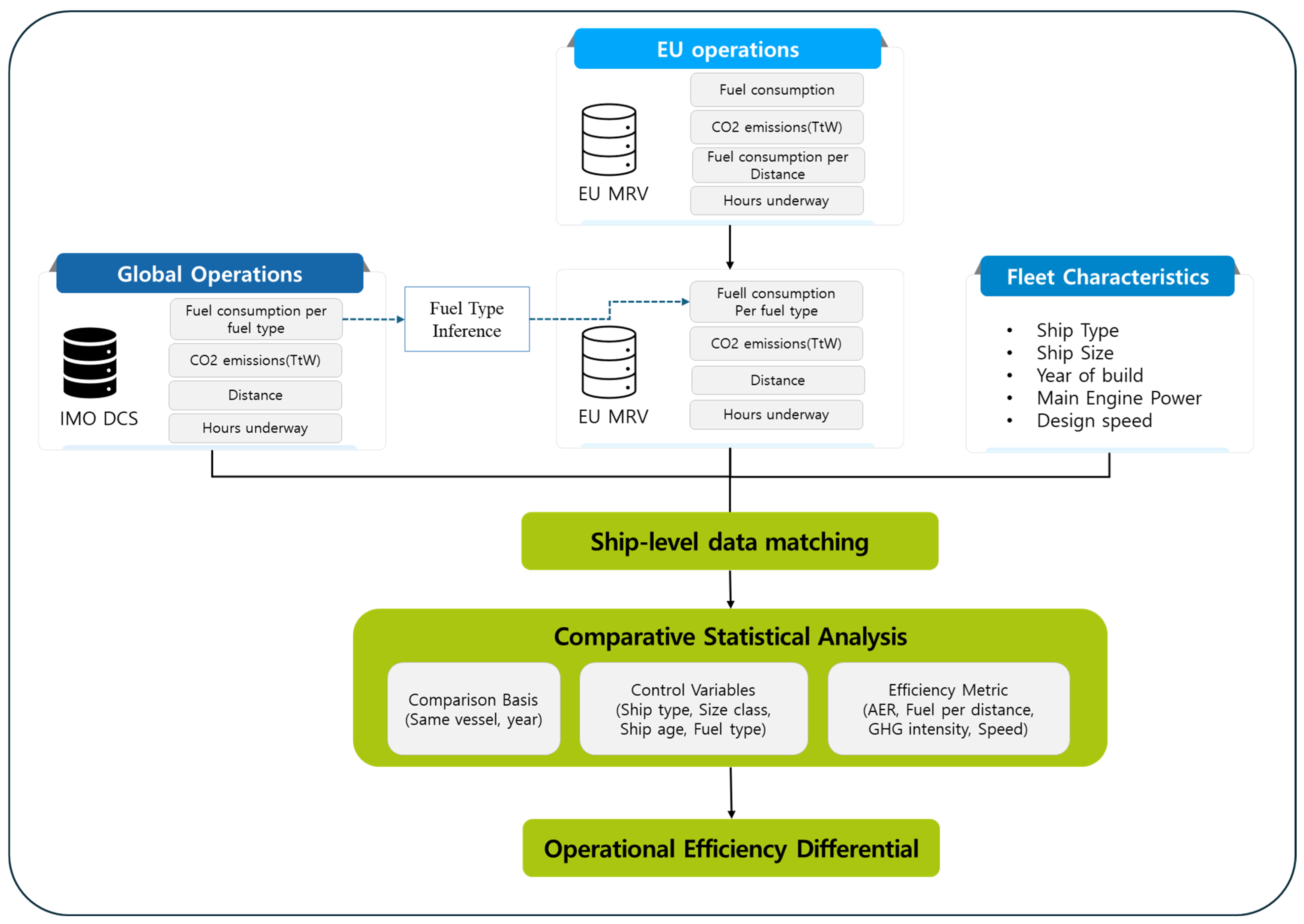
Figure 1 illustrates the analytical workflow, consisting of four sequential stages:

(1)

Data acquisition from the IMO DCS (global operations) and the EU MRV system (EU-related voyages);

(2)

Ship-level matching based on IMO number and calendar year;

(3)

Fuel type harmonization based on inference using DCS-reported fuel composition for matched vessels;

(4)

Computation and statistical comparison of operational efficiency metrics.

Because the EU MRV system does not provide fuel consumption disaggregated by fuel type, fuel type allocation for MRV records was inferred proportionally using corresponding DCS fuel type distributions for each matched vessel-year observation. The fleet characteristics of ship type, deadweight tonnage, build year, main engine power, and design speed were incorporated as control variables.

Comparative metrics included the Annual Efficiency Ratio (AER), fuel consumption per nautical mile, greenhouse gas intensity, and average operating speed. We used statistical analysis to quantify the magnitude and direction of efficiency differentials between global (DCS) and EU-related (MRV) operations.

4.1. Data Sources

Two regulatory datasets were employed in this study.

The IMO DCS dataset was obtained from the Global Integrated Shipping Information System (GISIS), which provides annual ship-level records of fuel consumption (disaggregated by fuel type), total distance traveled, and hours underway for global operations.

The EU MRV dataset was accessed via the THETIS-MRV platform operated by the European Maritime Safety Agency (EMSA). It provides verified annual ship-level totals of fuel consumption, CO₂ emissions, time at sea, cargo carried, and transport work for EU-related voyages.

The study period spans 2019–2024, covering six consecutive reporting years during which both monitoring systems operated in parallel. This period includes pre- and post-implementation phases of the CII regulation (effective from January 2023), enabling the assessment of temporal convergence patterns.

4.2. Ship Matching and Data Harmonization

Ship-level matching was performed using the IMO number as a unique identifier. Only observations appearing in both datasets within the same calendar year were retained. This one-to-one ship-year matching procedure ensures that differences reflect variation in operational context (global vs. EU-related voyages) rather than differences in fleet composition.

Observations with inconsistent or duplicate IMO identifiers were removed prior to matching. The matching process resulted in a balanced panel of vessels reported under both monitoring regimes.

Because the EU MRV dataset does not disclose fuel consumption disaggregated by fuel type, fuel type-specific components for MRV observations were harmonized using proportional fuel mix distributions derived from the corresponding DCS ship-year records. This proportional allocation preserves total reported fuel consumption while ensuring consistency in fuel-based emission calculations across systems.

The harmonization procedure assumes that the annual fuel composition reported under the DCS reasonably approximates the fuel mix used during EU-related voyages for the same vessel-year. Given the annual aggregation structure of both systems, this assumption is considered methodologically consistent for comparative intensity analysis.

4.3. Data Validation and Filtering

To ensure robustness and engineering plausibility, identical validation procedures were applied to both datasets prior to statistical comparison. The filtering process comprised three sequential stages.

First, ship-year observations with missing, zero, or non-positive values for key variables (fuel consumption, distance traveled, and deadweight tonnage) were excluded. This step removed approximately 2.3% of matched records.

Second, physically implausible operational profiles were removed using engineering-based thresholds. Observations were excluded if (i) the AER exceeded 50 gCO₂/dwt-nm (above the 99.9th percentile of the matched sample), (ii) the average sailing speed exceeded 30 knots, or (iii) the fuel consumption per nautical mile exceeded 1000 kg/nm. These thresholds were selected to eliminate extreme reporting anomalies rather than operational variability.

Third, statistical outliers were identified using the interquartile range (IQR) method. For each efficiency metric, observations outside the interval [Q1 – 3 × IQR, Q3 + 3 × IQR] were excluded. The 3 × IQR criterion was adopted to minimize excessive trimming while maintaining robustness against extreme distortions.

After filtering, the final analytical sample comprises between 50,055 and 50,079 ship-year observations (depending on metric-specific missing values), representing 15,755 unique vessels across 13 ship-type categories.

To assess the sensitivity of the results to the outlier filtering procedure, additional robustness checks were conducted using alternative filtering thresholds. Efficiency indicators were recomputed using the original dataset without filtering and a more restrictive filtering criterion (2 × IQR), in addition to the baseline 3 × IQR procedure. The resulting median differences between the DCS and the MRV system remained highly consistent across filtering specifications. For example, the median AER difference ranged from −0.156 to −0.163 gCO₂/dwt-nm across the three datasets, and fuel intensity and average speed differences exhibited similarly stable patterns.

Although mean values were slightly more sensitive to extreme observations when no filtering was applied, the median-based comparisons remained nearly unchanged. These results confirm that the observed DCS–MRV discrepancies are not driven by extreme outliers and that the statistical conclusions are robust to alternative filtering specifications.

4.4. Efficiency Indicator Definitions

Three operational efficiency indicators were constructed to evaluate cross-system consistency. The selection was based on three criteria: (1) methodological compatibility with both monitoring systems, (2) the availability of required variables in the DCS and MRV datasets, and (3) the complementary representation of ship operational performance.

(1) 

Annual Efficiency Ratio ($AER$)

The Annual Efficiency Ratio (AER) was adopted as the primary carbon intensity metric. The AER normalizes CO₂ emissions by transport work, expressed as the product of deadweight tonnage and distance traveled. This normalization enables inter-vessel comparability across different ship sizes and operational scales.

The AER is defined as

$$A\mathrm{E}\mathrm{R}={\displaystyle \frac{\mathsf{\Sigma }\left({\mathrm{F}\mathrm{C}}_{\mathrm{j}}\times {\mathrm{C}\mathrm{F}}_{\mathrm{j}}\right)}{\left(\mathrm{D}\mathrm{W}\mathrm{T}\times \mathrm{D}\right)}}$$

(1)

where the following apply:

• FC_j is the fuel consumption of fuel type j (tons);
• CF_j is the carbon emission factor for fuel type j (tCO₂/t-fuel);
• DWT is the deadweight tonnage (tons);
• D is the annual distance traveled (nautical miles).

By incorporating both energy consumption and transport activity, the AER reflects carbon intensity at the fleet-operational level and provides a standardized efficiency indicator for cross-system comparison.

(2) 

Fuel Intensity ($FI$)

Fuel intensity (FI) was introduced as a capacity-independent operational efficiency metric. Unlike the AER, which incorporates vessel capacity, FI isolates the direct relationship between fuel consumption and transport distance.

FI is defined as

$$FI=FC / D$$

(2)

where the following apply:

• FC is the total annual fuel consumption (tons);
• D is the distance traveled (nautical miles).

Fuel intensity is particularly sensitive to speed management practices, given the nonlinear relationship between propulsion power demand and vessel speed, typically approximated by a cubic function under steady-state hydrodynamic conditions.

(3) 

Average Operating Speed ($v$)

Average operating speed was included to assess whether efficiency differentials are associated with systematic variations in speed management. Since propulsion power and fuel consumption increase nonlinearly with speed, variations in average speed represent a primary driver of operational efficiency differences.

Average speed is defined as

$$v=D / T$$

(3)

where the following apply:

• D is the annual distance traveled (nautical miles);
• T is the total operating hours (hours).

Comparing average speed between the DCS (global operations) and MRV (EU-related voyages) datasets enables the identification of behavioral operational adjustments vs. reporting-induced discrepancies.

Collectively, the three indicators provide complementary perspectives on operational performance. The AER captures carbon intensity normalized by transport work, FI reflects direct energy consumption efficiency, and average speed serves as a behavioral proxy influencing both metrics. Their joint evaluation enables the multi-dimensional assessment of cross-system consistency.

The EEOI was not adopted due to limited cargo mass reporting consistency across MRV observations, which may introduce bias in transport work normalization.

4.5. Statistical Analysis Methods

The statistical comparison framework comprises four complementary procedures designed to evaluate cross-system consistency between DCS- and MRV-derived efficiency indicators.

(1) 

Paired Non-parametric Test

For each efficiency indicator X, paired differences were computed at the ship-year level as

$$\mathsf{\Delta }\mathrm{X}=X_{MRV}-X_{DCS}$$

(4)

where $X_{MRV}$ and $X_{DCS}$ denote the MRV- and DCS-derived values for the same vessel and calendar year.

The normality of the paired differences was assessed using the Shapiro–Wilk test. Given the large sample size and evidence of non-normality in several metrics, the Wilcoxon signed-rank test was adopted as the primary inferential method. This non-parametric test evaluates whether the median of the paired differences significantly deviates from zero without assuming a normal distribution.

(2) 

Effect Size Estimation

To quantify the magnitude of differences independent of sample size, Cohen’s d for paired samples was computed as

$$\mathrm{d}={\mu }_{∆}-{\sigma }_{∆}$$

(5)

where ${\mu }_{∆}$ is the mean of the paired differences and ${\sigma }_{∆}$ is the standard deviation of the paired differences.

Effect sizes were interpreted following conventional thresholds:

|d| < 0.2 (negligible);

0.2 <= |d| < 0.5 (small);

0.5 <= |d| < 0.8 (medium);

|d| >= 0.8 (large).

Given the large analytical sample (>50,000 observations), emphasis was placed on effect size magnitude rather than statistical significance alone.

(3) 

Bland–Altman Agreement Analysis

Agreement between the DCS and MRV indicators was evaluated using the Bland–Altman method. For each indicator, the mean bias and 95% limits of agreement (LoAs) were calculated as

$$Bias=mean\left(∆X\right)$$

(6)

$$LoA=Bias \pm 1.96\times SD\left(∆X\right)$$

(7)

This analysis enables the assessment of systematic bias and dispersion across the full measurement range and identifies whether discrepancies vary with indicator magnitude.

(4) 

Temporal Trend Analysis

To evaluate temporal convergence patterns, annual mean differences (ΔX) were computed for each reporting year from 2019 to 2024. Linear trend analysis was conducted to assess whether cross-system discrepancies decreased over time, particularly following the implementation of the CII regulation in 2023.

(5) 

Software

All statistical analyses were conducted using Python (version 3.11.2) with the SciPy, NumPy, and pandas libraries.

4.6. Stratified Consistency Analysis by Ship Type

To assess whether cross-system consistency varies across operational segments, the matched dataset was stratified by ship type. Vessel classifications from the DCS and MRV datasets were harmonized based on functional equivalence to ensure consistent grouping. The analysis included 13 ship-type categories: bulk carriers, oil tankers, chemical tankers, container ships, general cargo ships, LNG carriers, LPG carriers, ro-ro cargo ships, ro-ro passenger ships, cruise ships, vehicle carriers, refrigerated cargo ships, and other ship types.

For each ship type, efficiency indicators (AER, FI, and average speed) were computed separately for the DCS and MRV observations. Paired statistical comparisons and effect size estimations were then conducted within each category to quantify type-specific consistency patterns.

Stratification allows for the identification of systematic heterogeneity that may be obscured in aggregate-level analysis, particularly for vessel types characterized by distinct operational constraints or routing patterns.

Table 4. Summary of matched dataset characteristics.

Category	Value
Study period	2019–2024
Unique vessels	15,755
Total ship-year observations	50,055–50,079
Ship type categories	13
Data sources	IMO GISIS (DCS) and THETIS-MRV (MRV)
Matching criterion	IMO number + calendar year (one to one)
Efficiency indicators	AER, fuel intensity, and average speed

summarizes the dataset characteristics after matching and filtering.

5. Results and Analysis

In this section, we present the empirical findings of the comparative analysis of IMO DCS and EU MRV efficiency metrics. The results are organized into five subsections: validation of the estimation methodology, overall statistical agreement, distributional comparison, temporal trend analysis, and ship-type heterogeneity.

5.1. Validation of MRV-Based Emission Estimation

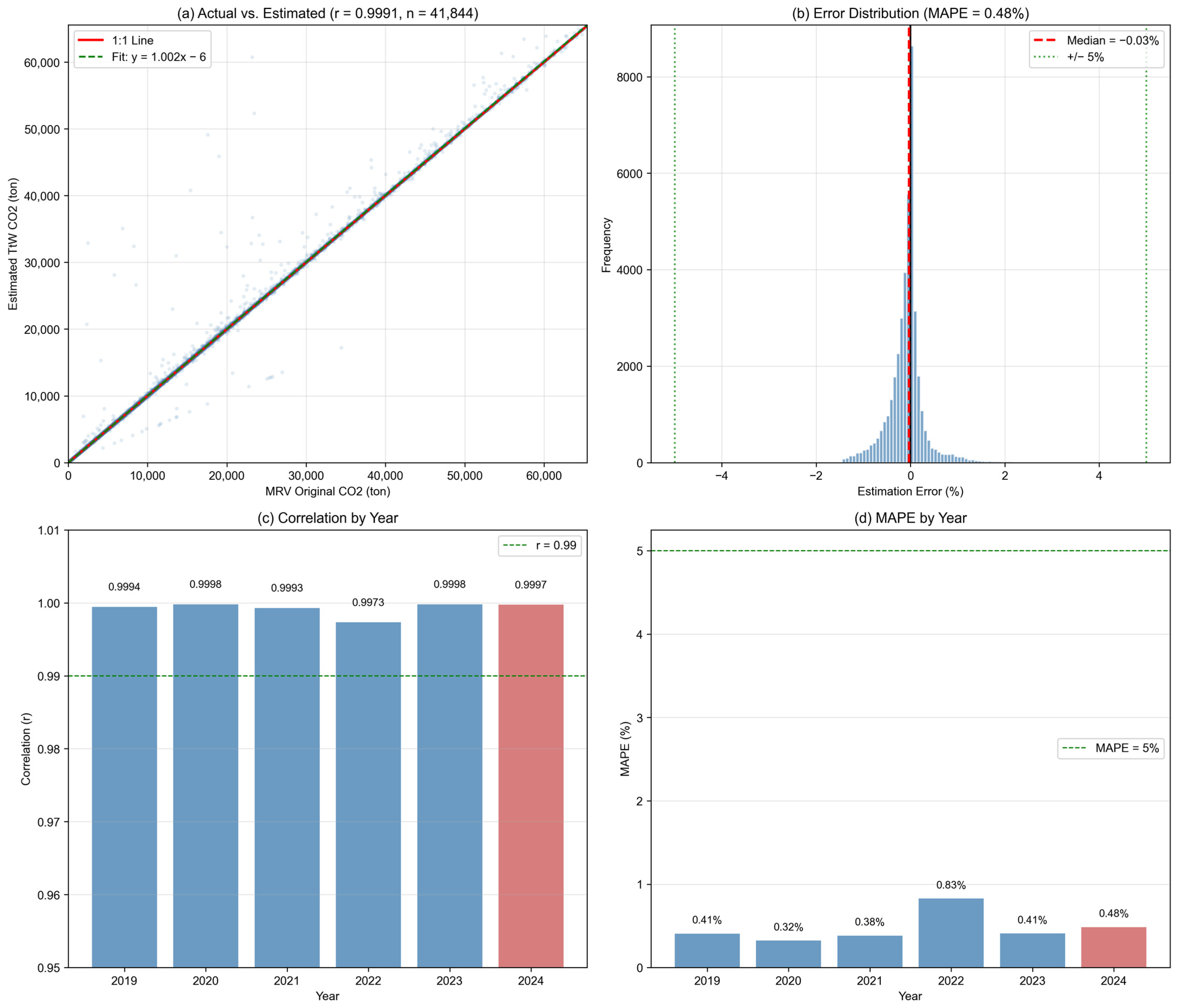
Because the EU MRV dataset does not provide fuel consumption disaggregated by fuel type, tank-to-wake (TtW) CO₂ emissions were reconstructed using proportional fuel mix distributions derived from matched DCS records. Prior to conducting cross-system comparisons, the accuracy of this reconstruction approach was evaluated against CO₂ emissions directly reported in the MRV dataset.

Table 5. Statistical validation of reconstructed MRV tank-to-wake CO₂ emissions.

Metric	Value
Sample size (paired observations)	41,844
Pearson correlation coefficient	0.9991
Median relative error	−0.03%
Mean absolute percentage error (MAPE)	0.48%
95th percentile absolute error	<2.5%

summarizes the key validation statistics based on 41,844 paired ship-year observations. The estimated and reported MRV CO₂ emissions exhibit near-perfect agreement, with a Pearson correlation coefficient of r = 0.9991, a median relative error of −0.03%, and a mean absolute percentage error (MAPE) of 0.48%. The 95th percentile absolute error remains below 2.5%, indicating that large estimation deviations are rare across the sample.

Figure 2 further illustrates these results. Annual correlation coefficients remain consistently above 0.997 across all years (2019–2024), with annual MAPE values ranging from 0.32% to 0.83%, confirming stable reconstruction performance over time.

These results indicate that proportional fuel mix harmonization introduces negligible systematic bias and does not materially distort emission estimates. The validation confirms the methodological soundness of the reconstruction procedure, thereby supporting its application in subsequent efficiency metric comparisons.

5.2. Overall Statistical Agreement Between DCS and MRV Datasets

Table 6. Paired statistical comparison of DCS-MRV efficiency indicators.

Indicator	Number of Ships	Mean (DCS)	Mean (MRV)	Mean Diff.	p-Value	Cohen’s d
AER (gCO2/dwt-nm)	50,079	7.82	7.71	−0.11	<0.001	−0.018
Fuel Intensity (kg/nm)	50,055	48.3	47.6	−0.68	<0.001	−0.015
Average Speed (knots)	50,062	11.42	11.28	−0.14	<0.001	−0.021

presents paired statistical comparison for the three efficiency indicators across the 50,000+ matched ship-year observations. Differences are defined as MRV minus DCS values.

All three indicators exhibit statistically significant paired differences (Wilcoxon signed-rank test, p < 0.001). However, given the large sample size, statistical significance alone does not imply substantive divergence. Effect size estimates indicate negligible magnitude differences across all indicators (|Cohen’s d| ≤ 0.021). According to conventional interpretation thresholds, these values fall well below the threshold for small effects (|d| = 0.2), suggesting that cross-system discrepancies are practically insignificant.

In absolute terms, MRV-based values are marginally lower than DCS-based values: the AER decreases by 0.11 gCO₂/dwt-nm (−1.4%), fuel intensity decreases by 0.68 kg/nm (−1.4%), and average speed decreases by 0.14 knots (−1.2%). The consistent direction of differences indicates slightly lower intensity and operating speed in EU-related voyages than in global operations. Nevertheless, the magnitude of these deviations remains minimal relative to overall fleet variability.

The combination of statistical significance with negligible effect size indicates that the two monitoring systems produce highly consistent representations of operational efficiency at the aggregate level.

5.3. Distributional Comparison and Agreement Analysis

Beyond mean-based comparisons, distributional characteristics were examined to determine whether observed differences arise from localized deviations within specific vessel segments or represent systematic shifts across the full operational spectrum.

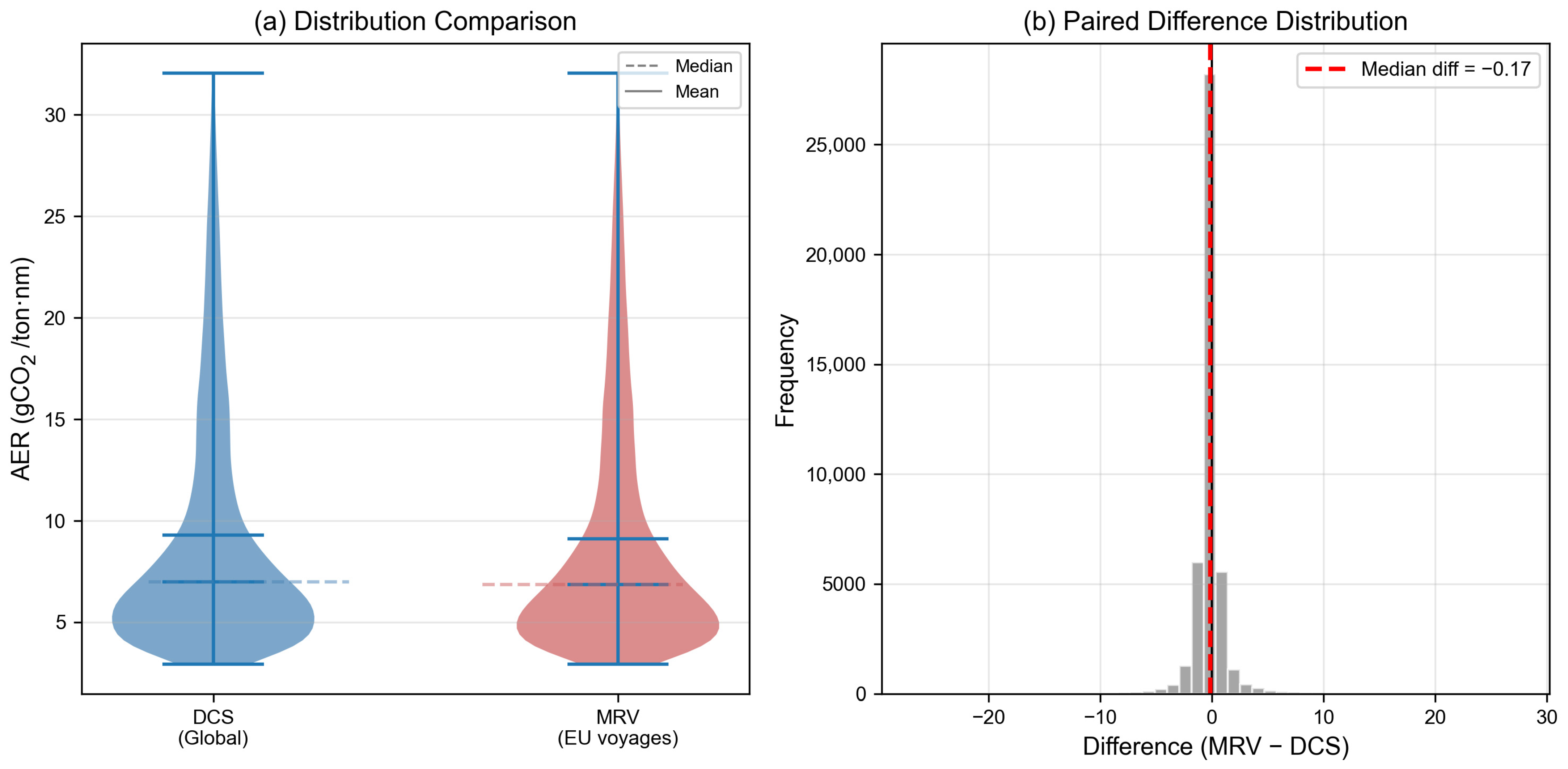
Figure 3 illustrates the distributional comparison of AER values between the DCS and MRV data. The two distributions exhibit substantial overlap across the entire range of observations. Median values are closely aligned (DCS: 5.94 gCO₂/dwt-nm; MRV: 5.86 gCO₂/dwt-nm), and interquartile ranges are nearly identical (DCS: 4.82; MRV: 4.76). Percentile analysis further confirms structural similarity. The 5th and 95th percentiles show minimal divergence (DCS: 2.15–18.42 gCO₂/dwt-nm; MRV: 2.12–18.21 gCO₂/dwt-nm), indicating that differences are not concentrated in either low- or high-intensity tails. The nearly indistinguishable distributional shapes suggest that the MRV distribution is marginally shifted downward relative to the DCS, rather than exhibiting structural distortion or segmentation-specific divergence.

Similar patterns were observed for fuel intensity and average speed. As presented in

Table 7. Distributional statistics for key efficiency indicators.

Indicator	Dataset	Median	IQR	5th Pctl	95th Pctl
AER (gCO2/dwt-nm)	DCS	5.94	4.82	2.15	18.42
	MRV	5.86	4.76	2.12	18.21
Fuel Intensity (kg/nm)	DCS	38.7	32.4	12.8	112.5
	MRV	38.2	31.9	12.6	111.2
Average Speed (knots)	DCS	11.85	3.24	7.42	15.68
	MRV	11.72	3.18	7.35	15.54

, for fuel intensity, median values differ by only 0.5 kg/nm (38.7 vs. 38.2 kg/nm), with overlapping interquartile ranges and nearly identical 90% percentile spans. Average speed distributions also demonstrate strong overlap, with median differences of 0.13 knots and comparable dispersion (IQR ≈ 3.2 knots for both datasets). Across all indicators, the MRV distributions exhibit a consistent but minor leftward shift relative to the DCS while preserving dispersion characteristics and tail symmetry.

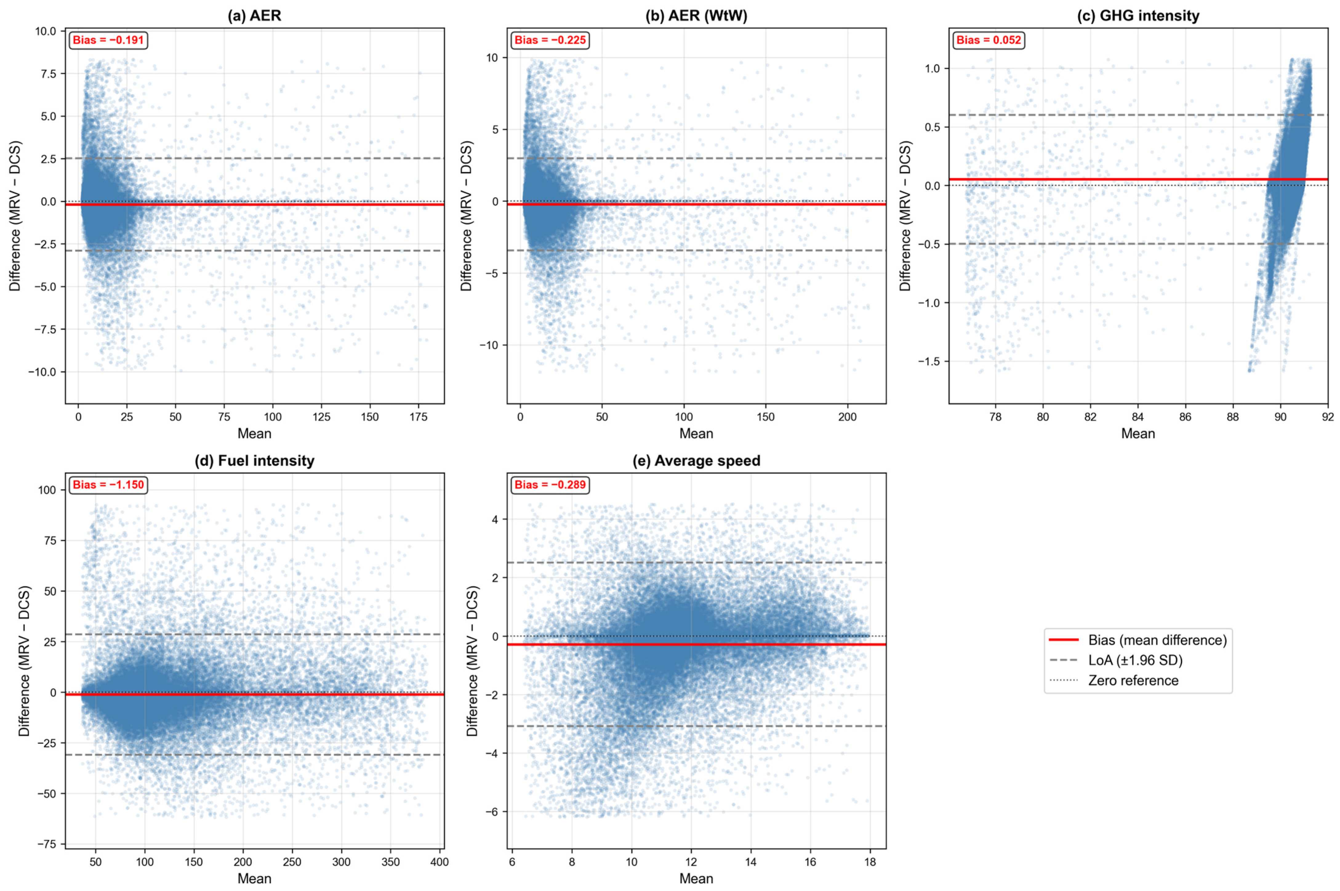
Bland–Altman analysis (Figure 4) further supports cross-system consistency. For all three indicators, mean biases are centered close to zero, and differences are symmetrically distributed around the bias line.

The 95% limits of agreement (LoAs) are as follows:

AER: −2.34 to +2.12 gCO₂/dwt-nm.

Fuel Intensity: −15.2 to +13.8 kg/nm.

Average Speed: −1.42 to +1.14 knots.

Importantly, no heteroscedastic pattern is observed; differences do not systematically increase with indicator magnitude. This indicates that discrepancies remain stable across low- and high-intensity vessels, reinforcing the conclusion that the observed deviations reflect minor uniform shifts rather than magnitude-dependent bias.

Collectively, the distributional and agreement analyses confirm that the DCS and MRV datasets exhibit structural equivalence at the fleet level, with only marginal and uniformly distributed deviations.

5.4. Temporal Trend Analysis (2019–2024)

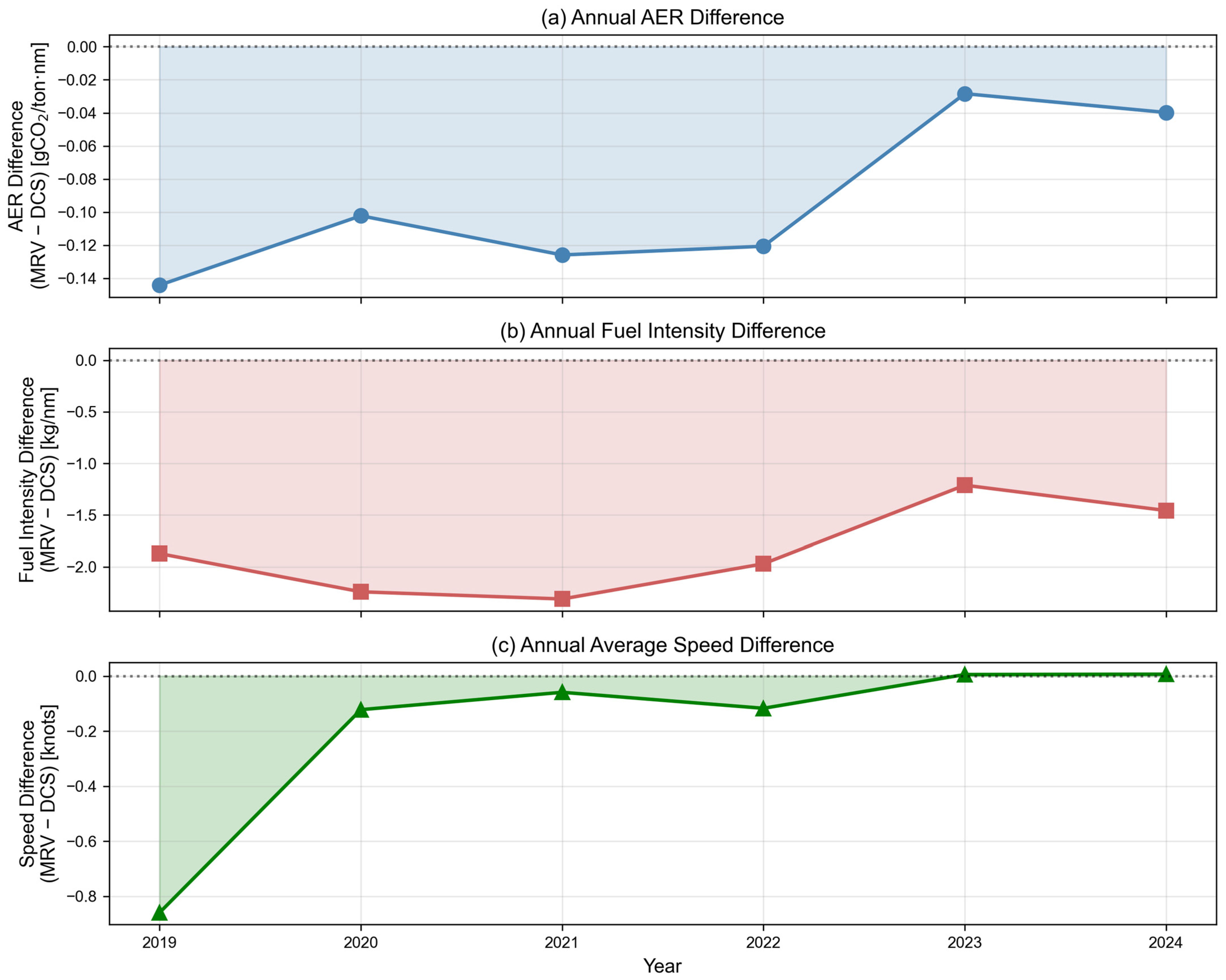
Figure 5 illustrates the annual evolution of mean paired differences (MRV − DCS) for the three efficiency indicators from 2019 to 2024. The objective of this analysis is to assess whether cross-system discrepancies exhibit convergence over time.

As shown in

Table 8. Annual mean differences (MRV—DCS) by year.

Year	AER Diff. (%)	Fuel Int. Diff. (%)	Speed Diff. (%)	Number of Ships
2019	−2.1	−2.0	−1.8	7842
2020	−1.8	−1.7	−1.5	8156
2021	−1.6	−1.5	−1.2	8423
2022	−1.3	−1.2	−0.9	8567
2023	−0.9	−0.8	−0.6	8612
2024	−0.6	−0.5	−0.4	8455

, the magnitude of differences decreases consistently across the study period. For the AER, the mean difference narrows from −2.1% in 2019 to −0.6% in 2024, representing a 71% reduction in relative divergence. Fuel intensity and average speed follow similar trajectories, with differences declining from −2.0% to −0.5% and from −1.8% to −0.4%, respectively.

Several notable patterns emerge from the temporal analysis.

First, the magnitude of DCS-MRV differences decreased progressively over the study period. The AER difference declined from −2.1% in 2019 to −0.6% in 2024, representing a 71% reduction in the gap between EU-related and global operational efficiency.

Second, the convergence pattern becomes more pronounced after 2022, coinciding with the implementation phase of the Carbon Intensity Indicator (CII) regulation in 2023. Although causality cannot be established within the scope of this study, the observed reduction in cross-system discrepancies suggests increasing alignment in operational behavior between global and EU-related voyages.

Third, speed differences exhibit the fastest rate of convergence, declining from −1.8% in 2019 to −0.4% in 2024. Given the nonlinear relationship between speed and fuel consumption, this reduction likely contributes to the narrowing gap observed in both the AER and fuel intensity.

Overall, the temporal analysis indicates progressive convergence of efficiency metrics between the DCS and the MRV system, reinforcing the robustness of cross-system comparability over time.

5.5. Ship-Type Heterogeneity

The matched dataset comprises 50,063 ship-year observations distributed across 13 vessel type categories. To assess whether cross-system consistency varies by operational segment, paired Wilcoxon signed-rank tests and Cohen’s d effect sizes were computed separately for each vessel type and efficiency indicator.

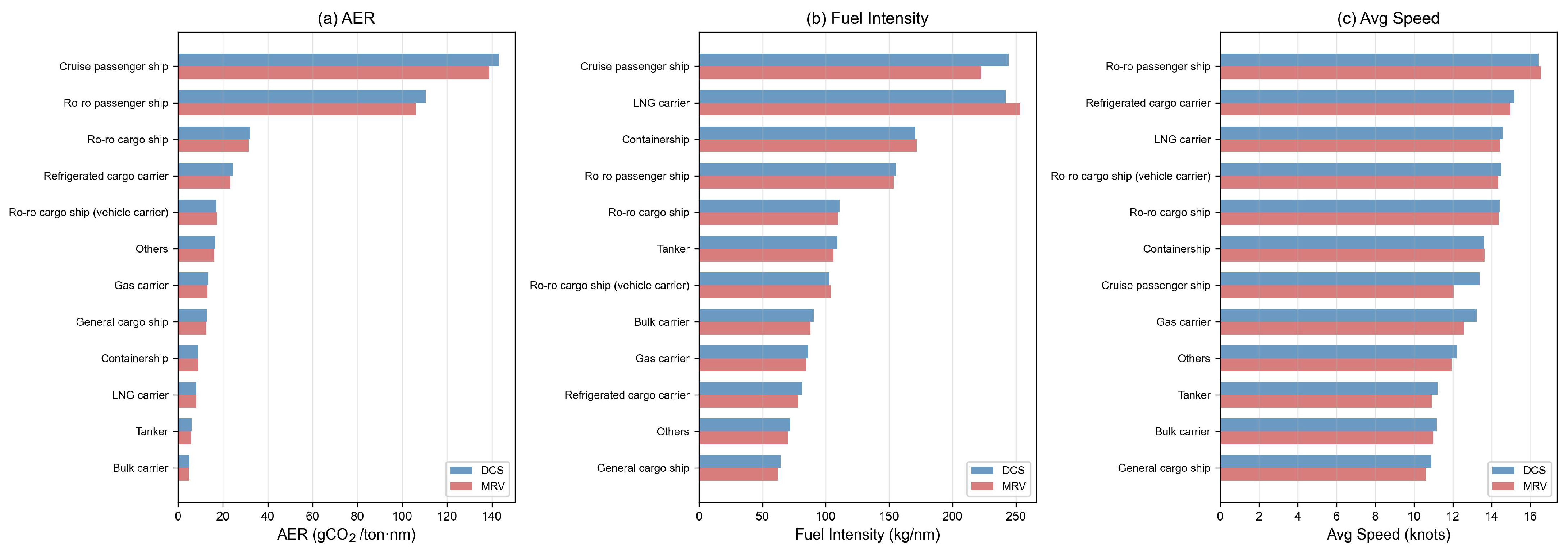
Figure 6 compares the median values of the AER, fuel intensity, and average speed between the DCS and MRV data for each vessel category. The results reveal systematic heterogeneity in cross-system differences. For most cargo vessel types (e.g., bulk carriers, oil tankers, chemical tankers, and general cargo ships), MRV-based medians are consistently lower than DCS-based medians across all indicators. In contrast, container ships exhibit near-identical median values between systems, while certain passenger-related vessel categories display either negligible differences or reversed patterns.

These results indicate that cross-system discrepancies are not uniformly distributed across vessel types, but instead reflect segment-specific operational characteristics.

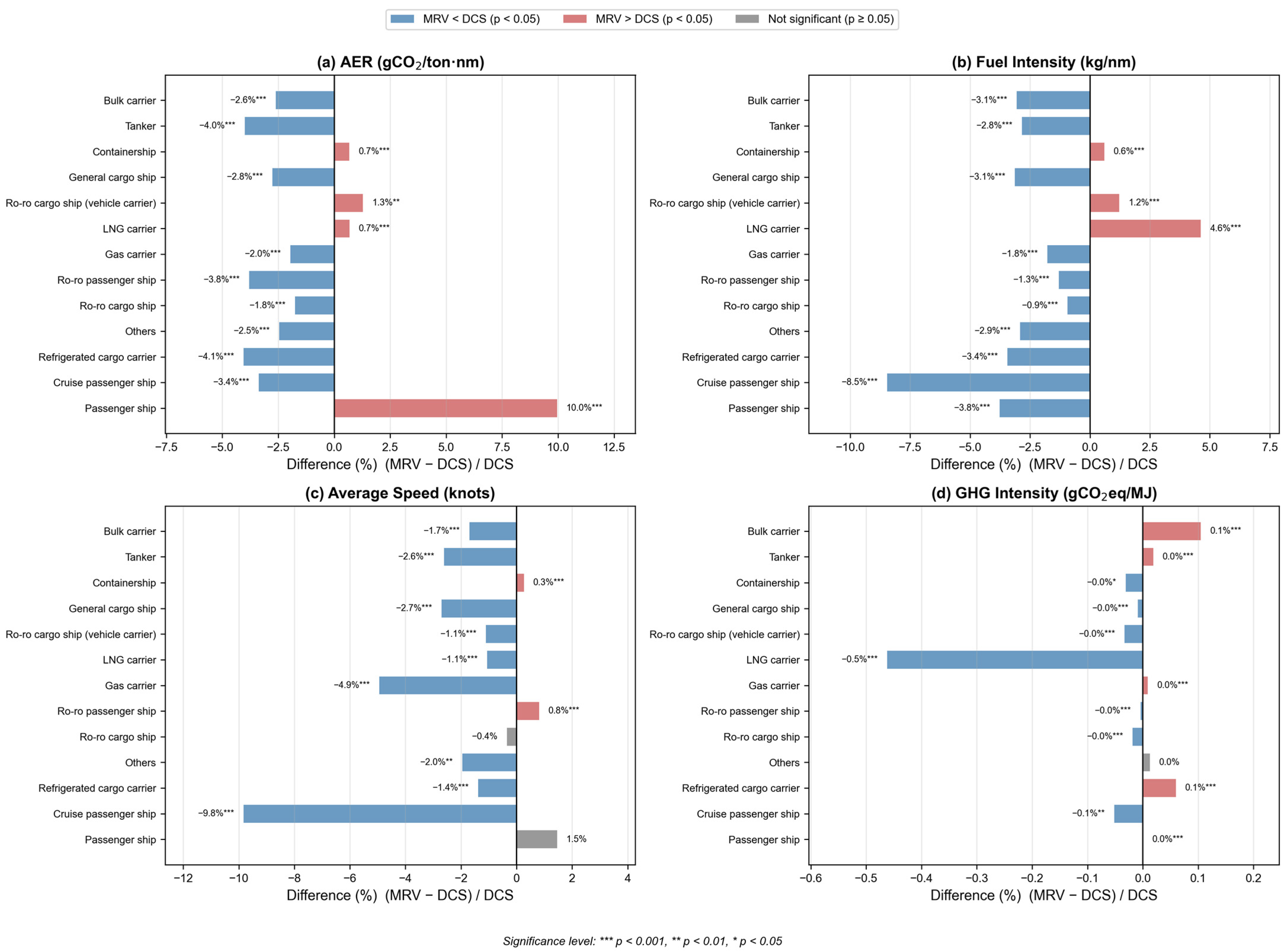
Figure 7 shows the differences between the MRV system and the DCS for each vessel type as percentages, together with statistical significance. Positive values indicate that MRV values are higher than DCS ones, while negative values indicate the opposite. Statistical significance is indicated through color coding: red represents MRV values being significantly higher than DCS ones, blue represents the opposite, and gray indicates no statistical significance.

(1)

AER (Annual Efficiency Ratio)

As shown in Figure 7a, AER differences vary substantially across vessel types. Refrigerated cargo ships exhibit the largest negative deviation (−4.05%), followed by tankers (−3.99%), ro-ro passenger ships (−3.80%), and cruise ships (−3.37%), all statistically significant (p < 0.001). Conversely, passenger ships display a pronounced positive deviation (+9.95%, p < 0.001), representing the largest divergence observed. Container ships and LNG carriers show minimal differences (+0.67% and +0.68%, respectively). The pronounced positive AER difference for passenger vessels can be explained by the structure of the AER formula, which normalizes emissions by DWT × distance. Shorter voyage distances and frequent port calls reduce the denominator, mechanically increasing the AER even when total fuel consumption remains comparable. This effect is particularly relevant for short-sea ferry operations within EU waters. In contrast, most cargo vessel categories exhibit consistent negative AER differences, indicating lower carbon intensity per transport work during EU-related voyages.

(2)

Fuel Intensity

Figure 7b shows vessel-type variation in fuel intensity differences. Cruise ships exhibit the largest reduction (−8.46%, p < 0.001), followed by refrigerated cargo ships (−3.44%), passenger ships (−3.77%), and general cargo ships (−3.13%). A notable exception is represented by LNG carriers, which display a +4.62% increase (p < 0.001). This divergence is attributable to boil-off gas (BOG) dynamics [23,24]. As voyage duration increases, natural cargo evaporation generates additional BOG [25]. When not fully utilized as propulsion fuel, this gas must be reliquefied or otherwise managed, increasing auxiliary energy consumption. Consequently, slower operations may increase total fuel usage despite reductions in average speed. Container ships and ro-ro cargo vessels exhibit minimal variation (≤1%), indicating strong cross-system consistency in operational profiles.

(3)

Average Speed

Figure 7c presents the differences in average operating speed by vessel type. Cruise ships exhibit the largest reduction in average speed (−9.83%, p < 0.001), representing the most pronounced change among all vessel categories. This pattern is consistent with the operational characteristics of cruise vessels, where itinerary design and onboard service experience often take precedence over strict arrival time optimization [26]. Moreover, given the high visibility of the cruise sector and its sensitivity to environmental reputation, operational adjustments in EU waters may reflect responsiveness to regional environmental regulations [27]. The complex itineraries involving multiple port calls further contribute to increased low-speed sailing segments [28]. Gas carriers also demonstrate a substantial reduction in speed (−4.94%, p < 0.001), while general cargo ships and tankers show moderate decreases of −2.70% and −2.62%, respectively. In contrast, ro-ro passenger ships and passenger ships exhibit slight increases in average speed (+0.81% and +1.45%, respectively). These increases may reflect the schedule-driven operational requirements typical of ferry services [29]. However, the speed increase observed for passenger ships was not statistically significant (p = 0.382), and the difference for ro-ro cargo ships was likewise non-significant (p = 0.778), indicating that such variations should be interpreted with caution.

(4)

GHG intensity

Figure 7d presents differences in well-to-wake (WtW) GHG intensity between DCS and MRV observations by vessel type. For most vessel categories, the differences remain within ±0.5%, indicating a high degree of consistency across the two regulatory datasets. This limited variation is primarily attributable to the dominance of conventional fossil fuels—such as HFO, VLSFO, and MGO—which account for more than 97% of fuel consumption in the study sample and exhibit relatively narrow WtW GHG intensity ranges (approximately 89–91 gCO₂eq/MJ).

An exception is observed for LNG carriers, which show a 0.46% reduction in GHG intensity under the MRV system (p < 0.001). This reduction is consistent with the lower WtW emission factor of LNG fuel (approximately 76–78 gCO₂eq/MJ) compared with conventional oil-based marine fuels. Unlike fuel intensity, which reflects total fuel consumed per distance traveled, GHG intensity is normalized by energy content and emission factors. Therefore, even if LNG carriers exhibit increased fuel intensity due to operational factors such as boil-off gas management and extended voyage durations, the inherent lower carbon intensity of LNG fuel results in a marginal reduction in overall WtW GHG intensity.

For other vessel types, the observed differences are minimal. Refrigerated cargo ships and bulk carriers show slight increases of 0.06% and 0.10%, respectively, which are statistically detectable but practically negligible. Overall, the narrow range of variation in GHG intensity confirms that differences between DCS and MRV observations are primarily operational rather than fuel-composition-driven for most vessel categories.

Figure 7 highlights vessel-type-specific heterogeneity in the differences between efficiency indicators derived from the DCS and MRV datasets. Across the majority of vessel categories, the indicator differences cluster within a narrow range, suggesting a generally consistent representation of operational efficiency across the two monitoring systems. However, certain vessel segments exhibit wider variability in the observed differences.

This pattern likely reflects structural operational characteristics associated with different vessel types. For example, vessels operating on more regular long-haul routes tend to show smaller discrepancies, whereas segments with more specialized operational profiles—such as LNG carriers or ro-ro vessels—may exhibit larger variability due to differences in voyage structure, cargo handling requirements, or fuel usage patterns. These findings indicate that cross-system discrepancies are more strongly associated with vessel-type-specific operational characteristics than with systematic inconsistencies between the reporting frameworks themselves. Overall, these results support the conclusion that the two monitoring systems provide broadly consistent representations of operational efficiency at the aggregated fleet level.

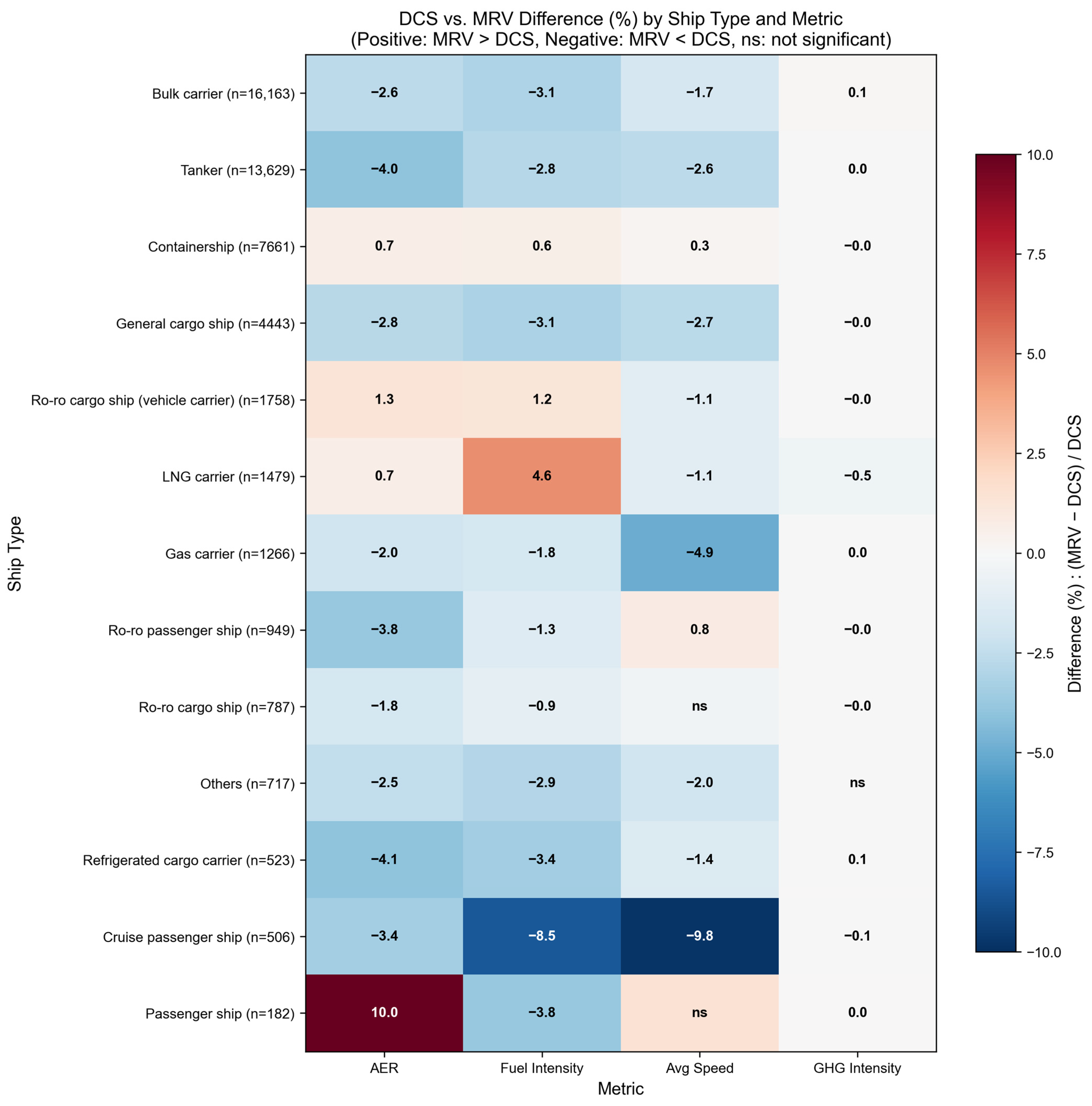
Figure 8 further summarizes these patterns using a heatmap representation of percentage differences between the MRV system and the DCS across vessel types and indicators. Each cell reflects the percentage difference for a given combination of vessel type–indicator, with red tones indicating that MRV values are higher than DCS ones and blue tones indicating the opposite. Statistically non-significant results are marked with “ns”.

Four dominant pattern groups emerge from the heatmap.

(1)

Vessel Types with Consistent Negative Differences

Bulk carriers (n = 16,163) exhibit consistently negative differences across all indicators, with the AER decreasing by 2.6%, fuel intensity by 3.1%, and average speed by 1.7% (p < 0.001). The large sample size confirms statistical robustness. The operational flexibility characteristic of tramp bulk shipping likely allows for speed adjustment and voyage optimization in EU waters [30,31].

Tankers (n = 13,629) show the largest AER reduction (−4.0%), accompanied by a 2.6% decrease in average speed. This pattern aligns with the well-established nonlinear relationship between speed and fuel consumption [32]. The reduction may be associated with operational adjustments under dense traffic and stricter navigational conditions in EU waters [33].

Refrigerated cargo ships (n = 523) display notable reductions (AER, −4.1%; fuel intensity, −3.4%) despite thermal management constraints, indicating that operational optimization remains feasible within technical limitations.

General cargo ships (n = 4443) also demonstrate consistent reductions (2.8–3.1%), reflecting the operational adaptability typical of tramp shipping segments.

(2)

Vessel Types with Minimal Differences

Container ships (n = 7661) exhibit negligible differences across all indicators (AER, +0.7%; fuel intensity, +0.6%; speed, +0.3%). Although statistically significant due to large sample size (p < 0.001), effect sizes remain extremely small (Cohen’s d ≤ 0.011). The standardized nature of liner operations and schedule rigidity likely constrain regional operational variation [34,35].

Ro-ro cargo ships (vehicle carriers; n = 1758) show small positive differences in AER (+1.3%) and fuel intensity (+1.2%), while average speed decreases by 1.1%. The modest efficiency deterioration despite reduced speed suggests that cargo handling characteristics and loading patterns may moderate the expected speed–fuel relationship.

(3)

Vessel Types with Extreme or Asymmetric Patterns

Cruise ships (n = 506) demonstrate the most pronounced changes. Average speed decreases by 9.8% (Cohen’s d = −0.418, medium effect size), and fuel intensity declines by 8.5%. These results indicate substantial operational adjustment in EU-related voyages. Cruise itineraries typically include multiple port calls and extended low-speed segments [26,28], which structurally differentiate them from cargo operations. The sector’s exposure to environmental scrutiny may also influence operational behavior [27].

Passenger ships (n = 182) exhibit a paradoxical pattern: the AER increases by 10.0% (p < 0.001), while fuel intensity decreases by 3.8% (p < 0.001). This divergence arises from the mathematical structure of the AER, where the denominator (DWT × distance) is substantially reduced in short-sea ferry routes. Thus, shorter voyage distances increase the AER even when absolute fuel consumption declines. The non-significant speed difference (p = 0.382) confirms schedule-driven operational constraints typical of ferry services [29].

LNG carriers (n = 1479) present another asymmetric pattern. Fuel intensity increases by 4.6% (p < 0.001), while average speed decreases by 1.1%, and WtW GHG intensity declines by 0.5% (Cohen’s d = −0.291). The increase in fuel intensity despite slower speeds is consistent with boil-off gas (BOG) dynamics, where longer voyage durations increase BOG generation and associated energy use [23,24,25]. However, the inherently lower WtW emission factor of LNG carriers relative to oil-based fuels results in a slight reduction in overall GHG intensity.

(4)

Vessel Types with Moderate or Mixed Patterns

Gas carriers (n = 1266) show a notable speed reduction (−4.9%; Cohen’s d = −0.200), while the AER and fuel intensity decrease more modestly (2.0% and 1.8%). This indicates that speed reduction does not translate proportionally into efficiency gains, likely reflecting cargo handling and safety constraints.

Ro-ro passenger ships (n = 949) display asymmetric behavior, with the AER decreasing by 3.8%, while average speed increases slightly (+0.8%). Efficiency improvements may stem from factors other than speed adjustment, such as loading optimization or routing patterns.

Ro-ro cargo ships (n = 787) show minimal differences, and the speed variation is not statistically significant (p = 0.778).

Wilcoxon tests of vessel types indicate statistical significance in most categories (p < 0.001), but both the magnitude and direction of differences vary systematically. Bulk carriers and tankers cluster in consistently negative differences, container ships display near-zero variation, and LNG carriers exhibit indicator-dependent divergence. The heatmap visualization clearly demonstrates that DCS–MRV differences are not uniformly distributed across the fleet but are structured by vessel-type-specific operational characteristics and constraints. Rather than indicating structural inconsistency between regulatory systems, these findings suggest that observed differences primarily reflect operational heterogeneity across maritime segments.

A synthesis of Figure 6, Figure 7 and Figure 8 indicates that DCS–MRV differences are structured by vessel-type-specific operational characteristics rather than random variation. Large tramp-operated cargo vessels (e.g., bulk carriers and tankers) exhibit consistent negative differences across indicators, suggesting that operational flexibility enables measurable efficiency adjustments in EU-related voyages. In contrast, container ships show minimal divergence, reflecting highly standardized liner operations. Certain vessel types, including LNG carriers and passenger ships, display asymmetric or indicator-dependent patterns, highlighting nonlinear operational dynamics. These observations confirm substantial inter-vessel heterogeneity, which is further examined in the Discussion section.

In addition to vessel-type heterogeneity, differences between DCS and MRV data may also be influenced by vessel size, as operational flexibility, routing patterns, and fuel consumption characteristics vary with ship scale. Larger vessels typically operate on long-haul routes with more stable operational profiles, whereas smaller vessels are more frequently engaged in regional or short-sea trades involving shorter voyage distances and higher port call frequency. These structural differences may affect efficiency indicators such as the AER, which is normalized by transport work (deadweight tonnage × distance).

Although the present study primarily examines heterogeneity at the vessel-type level, the large, matched sample inherently incorporates a broad distribution of vessel sizes across ship categories. Consequently, size-related operational variation is partially captured within the vessel-type segmentation framework. For example, bulk carriers and tankers in the dataset span a wide deadweight range from medium-size vessels to very large units, while container ships and LNG carriers tend to operate within more standardized size classes.

A preliminary inspection of the matched dataset indicates that the relative differences between DCS and MRV data remain broadly consistent across the size spectrum, suggesting that the observed discrepancies are primarily associated with operational characteristics of vessel segments rather than vessel scale itself. Future research using more granular vessel-size stratification may further clarify the interaction among ship size, operational behavior, and monitoring-system consistency.

6. Discussion

6.1. Implications for Monitoring-System Alignment

The central finding of this study—that the DCS and the MRV system produce statistically consistent efficiency metrics—provides empirical evidence relevant to ongoing discussions on regulatory alignment between global and regional maritime monitoring frameworks.

Although statistically significant differences are detected due to the large sample size, their magnitude remains small. The approximately 1.4% gap observed in the AER and fuel intensity, together with Cohen’s d values below 0.025, indicates that both monitoring systems capture broadly comparable representations of operational performance. From a technical perspective, this suggests that the two systems generate largely compatible efficiency assessments despite differences in geographic scope and reporting structure.

The temporal convergence observed over the 2019–2024 period further reinforces this interpretation. The 71% reduction in DCS–MRV differences following the implementation of the CII regulation in 2023 suggests that globally applied operational efficiency measures may contribute to narrowing regional operational variation. As additional lifecycle-based measures are progressively implemented at the international level, further alignment of operational patterns may occur.

At the same time, the vessel-type heterogeneity analysis indicates that DCS–MRV differences are not uniformly distributed across ship categories. While several cargo vessel segments exhibit relatively stable and consistent patterns, specialized vessel types—including LNG carriers, cruise ships, and passenger vessels—display indicator-dependent or asymmetric responses. These results suggest that any harmonization assessment should consider vessel-type-specific operational characteristics when interpreting comparative efficiency metrics.

Overall, the findings imply that differences between the DCS and the MRV framework are primarily operational rather than structural in nature. This supports the feasibility of analytical comparability between the two systems while highlighting the importance of accounting for segment-specific operational dynamics in regulatory evaluation.

6.2. Interpretation of Observed Differences

The consistently lower MRV values relative to the DCS ones across efficiency indicators warrant careful interpretation. The observed differences appear to be associated with operational and structural factors rather than methodological inconsistencies. Three explanatory dimensions emerge from the analysis, with varying relevance across vessel types.

First, the geographic characteristics of EU-related voyages may contribute to marginal efficiency differences for certain vessel categories. European port density and shorter voyage segments can reduce ballast exposure and enable more frequent routing optimization for tramp-operated vessels such as tankers and bulk carriers. These structural features are consistent with the moderate AER reductions (2.6–4.0%) observed in flexible cargo segments, whereas liner-operated container ships—characterized by fixed service patterns—exhibit minimal variation (approximately 0.7%).

Second, the regulatory environment in EU waters may be associated with more conservative operational behavior for specific vessel segments. Public disclosure under the EU MRV Regulation and the earlier implementation of regional climate measures may have influenced operational adjustments on EU-related routes. This pattern is most evident in cruise vessels, which demonstrate substantial speed and fuel intensity reductions. In contrast, schedule-constrained container services show negligible divergence, indicating limited regional operational flexibility.

Third, speed management differences appear to be a central mechanism underlying DCS–MRV divergence. Time-series results indicate that speed discrepancies exhibited the most rapid convergence over the study period, suggesting that early-stage regional slow-steaming practices became more uniformly adopted across global operations. However, this mechanism applies predominantly to vessel types with operational discretion; container ships maintained consistent speed profiles throughout the study period.

The temporal convergence observed after 2023 may be associated with behavioral adjustments following the implementation of the Carbon Intensity Indicator (CII) regulation. Unlike earlier monitoring frameworks that primarily focused on emission transparency, the CII introduces a globally applied operational performance rating based on annual carbon intensity. As a result, ship operators face increasing incentives to manage operational parameters such as sailing speed, routing efficiency, and fuel consumption across their entire trading network rather than only within specific regulatory regions.

Consequently, operational practices that were previously more pronounced in EU-related voyages—such as speed optimization or fuel management strategies—may have become more uniformly applied across both EU and non-EU operations. Such fleet-wide operational alignment may explain the progressive reduction in DCS–MRV discrepancies observed during the study period. While the present analysis does not establish causal attribution, the observed convergence pattern is consistent with the broader regulatory shift toward global operational efficiency management under the IMO framework.

The vessel-type heterogeneity analysis further clarifies these patterns. Segments with greater operational flexibility (e.g., tankers and bulk carriers) show clearer speed–efficiency linkage, while standardized liner services display structural rigidity. The indicator-dependent patterns observed for LNG carriers and passenger vessels highlight the importance of contextual interpretation. For example, LNG carriers exhibit increased fuel intensity alongside reduced speed due to boil-off gas dynamics, while passenger vessels show increased AERs but reduced fuel intensity due to the mathematical structure of the AER denominator in short-distance ferry operations.

Overall, the results suggest that DCS–MRV differences primarily reflect operational heterogeneity across vessel types rather than structural inconsistencies in reporting frameworks. The two systems, therefore, appear to capture comparable efficiency signals, albeit through slightly different operational exposure.

6.3. Limitations

Several limitations should be considered when interpreting the results of this study.

First, the MRV dataset accessed via THETIS does not provide fuel consumption disaggregated by fuel type. The reconstruction of fuel mix using matched DCS records, although validated with a low mean absolute percentage error (0.48%), introduces methodological dependence between datasets and may slightly attenuate true differences.

Second, the analysis is based on annual aggregated data and does not capture voyage-level variability. Intra-annual fluctuations related to seasonality, route structure, or cargo utilization cannot be directly observed within the available reporting framework.

Third, the study period (2019–2024) includes exceptional disruptions to global shipping patterns, particularly during the COVID-19 pandemic. Although temporal consistency was examined, abnormal operational conditions during this period may have influenced efficiency behavior.

Fourth, the matched-sample design inherently limits the analysis to vessels appearing in both the DCS and MRV datasets. Consequently, the results may not fully represent the complete global fleet reporting under either framework.

Despite these limitations, the large, matched sample and consistent patterns across indicators and vessel types support the reliability of the comparative findings.

6.4. Future Research Directions

The present study provides an empirical basis for further investigation of DCS–MRV consistency. Several extensions may enhance the understanding of regional and vessel-type-specific operational dynamics.

First, access to voyage-level data would enable more granular analysis of route characteristics, seasonality, and cargo utilization patterns underlying the aggregate differences observed in this study. Such analysis may clarify the mechanisms driving vessel-type-specific divergence.

Second, as lifecycle (well-to-wake) reporting expands under evolving EU and IMO frameworks, future work may examine how differences in fuel pathways and emission factors influence cross-system comparability. This will be particularly relevant for vessel types exhibiting indicator-dependent patterns, such as LNG carriers.

Third, longitudinal monitoring beyond the 2019–2024 period will be important to assess whether the convergence trend observed following CII implementation persists under subsequent regulatory developments.

Finally, as the global fleet transitions toward greater fuel diversity, comparative analyses incorporating alternative fuels will be necessary to evaluate whether increased variability in lifecycle emission intensity affects the consistency between these monitoring systems.

7. Conclusions

This study presents a large-scale empirical comparison of operational efficiency metrics derived from the IMO Data Collection System (DCS) and the EU Monitoring, Reporting and Verification (MRV) framework using matched ship-level observations. Based on 15,755 dual-reported vessels and more than 50,000 ship-year records between 2019 and 2024, we applied paired statistical methods, effect size estimation, and agreement diagnostics to evaluate cross-system consistency across multiple operational efficiency indicators.

The results indicate that the DCS and the MRV framework produce statistically consistent representations of operational efficiency. Although paired statistical tests reveal significant differences due to the large sample size, the magnitude of these differences is practically negligible. MRV-derived values are, on average, approximately 1.4% lower than DCS values in both AER and fuel intensity, and distributional analyses confirm substantial overlap across the two monitoring systems.

Temporal analysis further reveals progressive convergence between the two systems during the study period. The reduction in DCS–MRV differences after 2023 suggests increasing alignment of operational practices across global and EU-related voyages, potentially associated with the introduction of the Carbon Intensity Indicator (CII) regulation and the growing emphasis on fleet-level operational efficiency management.

At the same time, the analysis identifies pronounced vessel-type heterogeneity in cross-system differences. Flexible cargo segments such as bulk carriers and tankers exhibit consistent reductions in efficiency indicators during EU-related voyages, while container ships display near-zero variation due to the structural rigidity of liner service schedules. The indicator-dependent patterns observed in LNG carriers and passenger vessels highlight the importance of interpreting efficiency metrics within the operational context of specific vessel types.

From a regulatory perspective, the findings suggest that the DCS and MRV frameworks provide broadly comparable signals of operational performance despite differences in reporting scope and granularity. This supports the feasibility of analytical comparability across the two monitoring systems and indicates that combined datasets may be used for large-scale fleet efficiency analysis without introducing substantial structural bias.

More broadly, this study demonstrates the potential of large, matched regulatory datasets for the empirical validation of monitoring frameworks. As maritime decarbonization policies increasingly rely on operational data for compliance assessment and performance benchmarking, rigorous cross-system validation will become increasingly important for ensuring the reliability and interpretability of regulatory datasets.

References

1. International Maritime Organization. Fourth IMO GHG Study 2020; IMO: London, UK, 2020. [Google Scholar]
2. International Maritime Organization. MEPC.278(70)—Amendments to MARPOL Annex VI (Data Collection System for Fuel Oil Consumption of Ships); IMO: London, UK, 2016. [Google Scholar]
3. European Parliament and Council. Regulation (EU) 2015/757 on the Monitoring, Reporting and Verification of Carbon Dioxide Emissions from Maritime Transport. Official Journal of the European Union, L 123/55; European Parliament and Council: Brussels, Belgium, 2015. [Google Scholar]
4. Adamowicz, M. Decarbonisation of maritime transport—European Union measures as an inspiration for global solutions? Mar. Policy 2022, 145, 105282. [Google Scholar] [CrossRef]
5. International Maritime Organization. 2023 IMO Strategy on Reduction of GHG Emissions from Ships. Resolution MEPC.377(80); IMO: London, UK, 2023. [Google Scholar]
6. International Maritime Organization. MEPC.328(76)—2021 Revised MARPOL Annex VI (CII and EEXI Requirements); IMO: London, UK, 2021. [Google Scholar]
7. International Maritime Organization. MEPC.352(78)—2021 Guidelines on the Operational Carbon Intensity Reduction Factors Relative to Reference Lines (CII Reduction Factors Guidelines, G3); IMO: London, UK, 2021. [Google Scholar]
8. European Parliament and Council. Regulation (EU) 2023/1805 on the Use of Renewable and Low-Carbon Fuels in Maritime Transport (FuelEU Maritime). Official Journal of the European Union, L 234/48; European Parliament and Council: Brussels, Belgium, 2023. [Google Scholar]
9. European Parliament and Council. Directive (EU) 2023/959 Amending Directive 2003/87/EC Establishing a System for Greenhouse Gas Emission Allowance Trading (EU ETS Extension to Maritime). Official Journal of the European Union, L 130/134; European Parliament and Council: Brussels, Belgium, 2023. [Google Scholar]
10. Xing, H.; Chang, S.; Ma, R.; Wang, K. EU MRV Data-Based Review of the Ship Energy Efficiency Framework. J. Mar. Sci. Eng. 2025, 13, 1437. [Google Scholar] [CrossRef]
11. Zis, T.; Psaraftis, H.N. Operational measures to mitigate and reverse the potential modal shifts due to environmental legislation. Marit. Policy Manag. 2019, 46, 117–132. [Google Scholar] [CrossRef]
12. Psaraftis, H.N. Decarbonization of maritime transport: To be or not to be? Marit. Econ. Logist. 2019, 21, 353–371. [Google Scholar] [CrossRef]
13. Yeo, S.; Kim, J.K.; Choi, J.H.; Lee, W.J. Estimation of greenhouse gas emissions from ships registered in South Korea based on activity data using the bottom-up approach. Proc. Inst. Mech. Eng. Part M J. Eng. Marit. Environ. 2024, 238, 738–749. [Google Scholar] [CrossRef]
14. Zhang, C.; Zhu, J.; Guo, H.; Xue, S.; Wang, X.; Wang, Z.; Chen, T.; Yang, L.; Zeng, X.; Su, P. Technical Requirements for 2023 IMO GHG Strategy. Sustainability 2024, 16, 2766. [Google Scholar] [CrossRef]
15. Panagakos, G.; de Sousa Pessôa, T.; Dessypris, N.; Barfod, M.B.; Psaraftis, H.N. Monitoring the Carbon Footprint of Dry Bulk Shipping in the EU: An Early Assessment of the MRV Regulation. Sustainability 2019, 11, 5133. [Google Scholar] [CrossRef]
16. Luo, X.; Yan, R.; Wang, S. After five years’ application of the European Union monitoring, reporting, and verification (MRV) mechanism: Review and prospectives. J. Clean. Prod. 2024, 434, 140100. [Google Scholar] [CrossRef]
17. Park, G.; Cho, K. A study on the change of EEOI before and after modifying bulbous at the large container ship adopting low speed operation. J. Korean Soc. Mar. Eng. 2017, 41, 15–20. [Google Scholar] [CrossRef]
18. Kwon, B.J.; Jeong, B.U.; Lee, S.B.; Park, Y.M.; Oh, S.J.; Shin, S.C. Comparative analysis of EU ETS, FuelEU maritime and IMO carbon pricing regulations: Strategic and economic implications for the shipping industry. J. Adv. Mar. Eng. Technol. 2025, 49, 224–238. [Google Scholar] [CrossRef]
19. Jung, S.H. Study on characteristics of GHG life cycle assessment for alternative marine fuels. J. Adv. Mar. Eng. Technol. 2021, 45, 334–338. [Google Scholar] [CrossRef]
20. Psaraftis, H.N.; Kontovas, C.A. Decarbonization of Maritime Transport: Is There Light at the End of the Tunnel? Sustainability 2021, 13, 237. [Google Scholar] [CrossRef]
21. International Maritime Organization. Report of the Marine Environment Protection Committee on Its Eighty-Third Session (MEPC 83); IMO: London, UK, 2025. [Google Scholar]
22. International Maritime Organization. 2024 Guidelines on Life Cycle GHG Intensity of Marine Fuels. Resolution MEPC.391(81); IMO: London, UK, 2024. [Google Scholar]
23. Kulitsa, M.; Wood, D.A. Boil-off gas balanced method of cool down for liquefied natural gas tanks at sea. Adv. Geo-Energy Res. 2020, 4, 199–206. [Google Scholar] [CrossRef]
24. Jeong, S.; Jeong, D.; Park, J.; Kim, S.; Kim, B. A voyage optimization model of LNG carriers considering boil-off gas. In Proceedings of the OCEANS 2019 MTS/IEEE SEATTLE, Seattle, WA, USA, 27–31 October 2019; pp. 1–7. [Google Scholar]
25. Fernández, I.A.; Gómez, M.R.; Gómez, J.R.; Insua, Á.B. Review of propulsion systems on LNG carriers. Renew. Sustain. Energy Rev. 2017, 67, 1395–1411. [Google Scholar] [CrossRef]
26. Klein, R.A. Responsible cruise tourism: Issues of cruise tourism and sustainability. J. Hosp. Tour. Manag. 2011, 18, 107–116. [Google Scholar] [CrossRef]
27. Transport & Environment. One Corporation to Pollute Them All: Luxury Cruise Giant Emits 10 Times More SOx than All of Europe’s Cars; T&E Campaign Report: Brussels, Belgium, 2023. [Google Scholar]
28. Psaraftis, H.N.; Kontovas, C. Balancing the economic and environmental performance of maritime transportation. Transp. Res. Part D 2010, 15, 458–462. [Google Scholar] [CrossRef]
29. Zis, T.P.V.; Psaraftis, H.N. The implications of the new sulphur limits on the European Ro-Ro sector. Transp. Res. Part D 2017, 52, 185–201. [Google Scholar] [CrossRef]
30. Stopford, M. Maritime Economics, 3rd ed.; Routledge: London, UK, 2009. [Google Scholar]
31. Christiansen, M.; Fagerholt, K.; Nygreen, B.; Ronen, D. Ship routing and scheduling in the new millennium. Eur. J. Oper. Res. 2013, 228, 467–483. [Google Scholar] [CrossRef]
32. Adland, R.; Cariou, P.; Wolff, F.C. Optimal ship speed and the cubic law revisited: Empirical evidence from an oil tanker fleet. Transp. Res. Part E Logist. Transp. Rev. 2020, 140, 101972. [Google Scholar] [CrossRef]
33. Fagerholt, K.; Gausel, N.T.; Rakke, J.G.; Psaraftis, H.N. Maritime routing and speed optimization with emission control areas. Transp. Res. Part C 2015, 52, 57–73. [Google Scholar] [CrossRef]
34. Pasha, J.; Dulebenets, M.A.; Kavoosi, M.; Abioye, O.F.; Theophilus, O.; Wang, H.; Kampmann, R.; Guo, W. Holistic tactical-level planning in liner shipping: An exact optimization approach. J. Shipp. Trade 2020, 5, 8. [Google Scholar] [CrossRef]
35. Notteboom, T.E. The time factor in liner shipping services. Marit. Econ. Logist. 2006, 8, 19–39. [Google Scholar] [CrossRef]
Figure 1. Analytical workflow for cross-system comparison between IMO DCS and EU MRV datasets. Framework includes data acquisition, ship-level matching, fuel type harmonization, efficiency metric computation, and statistical consistency evaluation.
Applsci 16 02911 g001
Figure 2. Validation of reconstructed MRV tank-to-wake CO2 emissions. (a) Scatter plot of reported vs. reconstructed emissions with 1:1 reference line. (b) Distribution of relative reconstruction errors. (c) Annual Pearson correlation coefficients. (d) Annual mean absolute percentage error (MAPE).
Applsci 16 02911 g002
Figure 3. Distributional comparison of AER between DCS and MRV. (a) Violin plots showing the overall distribution of AER for each scheme; (b) Histogram of paired differences (MRV—DCS).
Applsci 16 02911 g003
Figure 4. Bland–Altman agreement analysis comparing DCS and MRV efficiency indicators. Plots show differences against mean values for AER, fuel intensity, and average speed. Solid lines indicate mean bias; dashed lines denote 95% limits of agreement.
Applsci 16 02911 g004
Figure 5. Temporal evolution of differences between MRV and DCS across key operational efficiency indicators (2019–2024). (a) Annual Efficiency Ratio; (b) fuel intensity; (c) average speed. Negative values indicate lower values under MRV system.
Applsci 16 02911 g005
Figure 6. Comparison of DCS and MRV median values by vessel type. (a) AER (gCO2/ton-nm), (b) fuel intensity (kg/nm), and (c) average speed (knots). DCS (blue); MRV (red).
Applsci 16 02911 g006
Figure 7. Percentage differences between DCS and MRV values by vessel type and statistical significance. (a) AER, (b) fuel intensity, (c) average speed, and (d) GHG intensity. Colors indicate statistical significance, with significance levels denoted by *** p < 0.001, ** p < 0.01, and * p <0.05.
Applsci 16 02911 g007
Figure 8. Heatmap of DCS-MRV differences by vessel type. Each cell represents the percentage difference for the corresponding combination of vessel type–indicator.
Applsci 16 02911 g008