Camera Pose Revisited

Abstract

Estimating the position and orientation of a camera with respect to an observed scene remains a fundamental problem in computer vision, particularly in calibration procedures and multi-sensor vision systems. This paper revisits the planar Perspective–n–Point (PnP) problem with emphasis on rotation representation, initialization strategy, and optimization behavior. We propose the PnP-ProCay78 algorithm, which combines analytical elimination of translation via quadratic reconstruction error with nonlinear least-squares minimization of projection residuals in Cayley parameter space. A deterministic initialization scheme based on canonical directions of the reconstruction matrix eliminates the need for spectral search over the full solution space. Experimental evaluation on heterogeneous datasets acquired from high-resolution RGB cameras and low-resolution thermal cameras demonstrates that the proposed method achieves reprojection accuracy comparable to state-of-the-art OpenCV implementations such as SQPnP and IPPE. Convergence analysis in Cayley space reveals stable and rapidly contracting optimization trajectories, with consistent behavior across sensors of significantly different resolution and noise characteristics. The results indicate that a carefully chosen rotation parameterization combined with a transparent optimization framework can yield competitive numerical performance while maintaining geometric interpretability and structural simplicity.

1. Introduction

Estimating the position and orientation of a camera with respect to an observed scene is one of the fundamental problems in computer vision and photogrammetry [1,2]. This task, commonly referred to as camera pose estimation, constitutes a key component of many image processing systems, including three-dimensional reconstruction, augmented reality, mobile robotics, visual navigation systems, and camera calibration procedures [3]. In the classical formulation, the problem reduces to determining a rigid (isometric) transformation between the camera coordinate frame and the scene reference frame based on known correspondences between three-dimensional points and their two-dimensional image projections.

One of the most frequently studied variants of this problem is the Perspective–n–Point (PnP) problem, in which the intrinsic parameters of the camera are assumed to be known, and the goal is to estimate its position and orientation from a finite set of 3D–2D correspondences. However, in this research we consider only planar calibration objects and hence the correspondences are 2D-2D only.

Despite decades of research and the availability of numerous algorithms with well-established theoretical properties, the PnP problem remains an active area of investigation. This is largely due to the inherent trade-offs between numerical stability, estimation accuracy, and computational complexity.

In practical library implementations, algorithms based on specialized optimization procedures or elaborate algebraic constructions currently dominate. While such methods often achieve excellent reconstruction accuracy, their internal structure can be difficult to analyze geometrically and to interpret intuitively. As a consequence, their transparency and pedagogical value are frequently limited. We observed this also in the case of the excellent state-of-the-art algorithm OpenCV-SQPnP of Terzakis and Lourakis [4] which inspired us to make this research.

In this work, we adopt the perspective of revisiting the camera pose estimation problem, focusing not only on the final value of the cost function but also on the structure of the solution space, the choice of rotation parameterization, and the behavior of the optimization process itself. In particular, we consider representing camera orientation in Cayley space, a classical concept originating from early studies on the theory of rotations [5,6], which exhibits favorable properties in the context of nonlinear optimization in contrast to other approaches to rotation parametrization using quaternions or exponential maps [7]. For a more detailed discussion of the Cayley representation, including historical and terminological issues, see Appendix A.

Based on this formulation, we propose the PnP-ProCay78 algorithm, which casts the camera pose estimation task as a least-squares problem solved using standard nonlinear optimization techniques. The proposed approach enables competitive camera pose estimation while maintaining a clear algorithmic structure and an intuitive geometric interpretation, making it attractive both for practical applications and for academic teaching.

2. Main Contributions

This paper presents a re-examination of the problem of camera pose and orientation estimation, with particular emphasis on the structure of the solution space, the choice of rotation representation, and the transparency of the optimization process. The main contributions of this work can be summarized as follows:

• A coherent and geometrically interpretable formulation of the camera pose estimation problem is proposed based on the Cayley parametrization. This representation eliminates the need for explicitly enforcing positive determinant and orthogonality constraints on the rotation matrix and enables a direct analysis of optimization trajectories in the parameter space.
• The PnP-ProCay78 algorithm is developed, in which the Perspective–n–Point problem is formulated and solved as a nonlinear least-squares task using standard optimization methods, without resorting to specialized algebraic solvers or procedures dedicated exclusively to this problem.
• An initialization strategy based on two antipodal starting trajectories in the Cayley space is introduced. This significantly increases the robustness of the algorithm to unfavorable initial conditions and enables reliable convergence to the global minimum of the cost function over a wide range of geometric configurations.
• An alternative interpretation of the Cayley space is presented by decomposing the state vector into a directional component and a norm component. This leads to an intuitive visualization of optimization trajectories in terms of projections into the unit disk and distances from the origin. Such a representation proves particularly useful for geometric analysis and academic teaching.
• An experimental evaluation of the proposed approach is conducted in comparison with reference algorithms included in OpenCV library, demonstrating practically the same or higher estimation accuracy while maintaining a simpler algorithmic structure and full compatibility with commonly used geometric models and optimization tools.
• In the context of multisensor vision systems, a preliminary synchronous analysis of the optimization convergence is presented for a pair of RGB and thermal cameras operating within a single hardware setup. Despite substantial differences in image resolution and point localization accuracy between the two sensors, the PnP-ProCay78 algorithm enables a consistent analysis of optimization trajectories within the same parameter space. At this stage, the analysis is visual and exploratory in nature, serving as a starting point for further research on convergence assessment in RGB–IR systems.

The presented results indicate that an appropriate choice of rotation representation combined with a conscious use of standard nonlinear optimization techniques makes it possible to construct a camera pose estimation algorithm that achieves high numerical quality while retaining conceptual clarity and strong didactic value, and that naturally fits within the framework of modern integrated vision systems.

3. Related Work

The development of algorithms for camera position and orientation estimation has progressed in parallel with advances in geometric modeling of the relationships between three-dimensional scenes and their image projections.

The earliest approaches to the Perspective–n–Point problem and the camera pose estimation problems were comprehensively described in the classical monographs by Hartley and Zisserman [1] as well as by Ma et al. [2], which to this day constitute the theoretical foundation for most contemporary algorithms.

The earliest approaches to the Perspective–n–Point problem were primarily based on algebraic solutions, often relying on minimal point configurations. The classification of solutions to the P3P problem presented by Gao et al. [8,9] together with the introduction of robust estimation techniques such as RANSAC proposed by Fischler and Bolles [10] enabled practical applications of camera pose estimation. However, these methods exhibited sensitivity to measurement noise and to geometric configurations close to degeneracy.

With the increasing availability of point correspondences, research shifted toward methods exploiting redundant data and formulating the PnP problem as an optimization task. A significant milestone in this direction was the EPnP algorithm proposed by Lepetit, Moreno-Noguer, and Fua [11], which allowed efficient processing of large point sets while maintaining low computational complexity. Subsequent works, such as the Direct Least Squares (DLS) method introduced by Hesch and Roumeliotis [12], focused on improving numerical stability and estimation accuracy.

In parallel, approaches tailored to scenes with specific geometric structures—most notably planar as in the work of Sturm and Maybank [13], frequently encountered in calibration tasks—were developed. In this context, the seminal works of Zhang [14] played a central role, followed by methods exploiting homography-based formulations and the separation of rotation and translation estimation. Among these, the IPPE algorithms proposed by Collins and Bartoli [15] have found widespread use in practical library implementations.

In recent years, particular attention has been paid to algorithms that combine high estimation accuracy with robustness to near-degenerate configurations. A representative example is the SQPnP algorithm introduced by Terzakis and Lourakis [4], which employs sequential quadratic programming to compute a globally optimal solution. While such methods achieve excellent numerical performance, they rely on complex, highly specialized optimization procedures, which complicates geometric analysis and interpretation of the estimation process.

Regardless of the specific PnP algorithm employed, the representation of three-dimensional rotations remains a critical issue. Commonly used representations include Euler angles, quaternions, and Lie algebra-based formulations, whose properties have been extensively surveyed, among others, by Shuster [16]. The Cayley representation, originally introduced in the classical work of Arthur Cayley [5], has so far been used relatively rarely in practical camera pose estimation algorithms, despite its favorable properties in the context of nonlinear optimization.

In the context of modern multi-sensor vision systems, increasing attention has also been devoted to camera pose estimation problems involving sensors with significantly different characteristics, such as RGB and thermal cameras. Studies on calibration and synchronization of such systems indicate that differences in resolution and data quality have a substantial impact on the behavior of estimation algorithms. Thermal mapping in multi-sensor systems has been extensively investigated, for example, by Borrmann et al. [17].

Against this background, the approach proposed in the present work fits within the class of nonlinear optimization-based methods, while distinguishing itself through a deliberate choice of the Cayley parameterization and a strong emphasis on geometric analysis and interpretability of the estimation process. These aspects are particularly relevant in the context of multi-sensor systems and educational applications.

An important perspective that emerges when revisiting classical PnP algorithms is the distinction between the application-level performance metrics and the internal error (loss) function optimized by a given method. In practical vision systems, the quality of pose estimation is ultimately assessed using the projection error measured in the projection plane or reprojection error measured in the sensor plane. In this work, projection error metrics are used for optimization, whereas reprojection error is employed solely for presenting results in pixel units. Note that the reprojection errors are obtained from projection errors by multiplying them by the focal length expressed in pixels. The latter is estimated from the sensor resolution and the angle of view of the lens used.

However, most efficient PnP solvers do not minimize the projection error directly, but instead rely on surrogate cost functions that admit more favorable analytical or computational properties like reconstruction error. They are defined, for example, in [4] as follows: for a set of point correspondences $(P_i,p_i)$, i.e., for a world object point $P_i$ and its projection point $p_i$, respectively, the error of pose $(R,t)$ is evaluated:

• Projection error:

  $${\mathcal{E}}_0^2\doteq \sum _i{∥p_i-{\displaystyle \frac{(R{P}_i+t)}{{(R{P}_i+t)}_z}}∥}^2.$$
• Reconstruction error:

  $${\mathcal{E}}^2\doteq \sum _i{∥p_i·{(R{P}_i+t)}_z-(R{P}_i+t)∥}^2.$$

This separation between the target metric and its optimization surrogate closely resembles a paradigm well known from modern machine learning, where task-level metrics are often replaced by differentiable or convex proxy losses. In the context of PnP, such surrogates include algebraic errors, quadratic reconstruction errors, or linearized residuals, which enable closed-form solutions or fast convergence of iterative solvers.

For instance, while methods such as EPnP formulate pose estimation using algebraic constraints derived from control points, they do not explicitly optimize the projection error. However, to fit the control points, a Gauss–Newton optimizer is used. Plane-based approaches such as IPPE exploit homography properties giving the closed formula solutions with respect to reference functions like svd, rank. This means that surrogate loss functions are implicitly embedded in matrix diagonalization procedures like finding singular values in svd. More recent methods, including DLS and SQPnP, explicitly introduce cost functions that approximate the projection error while remaining amenable to efficient global or near-global optimization. In 

Table 1. Relationship between the application-level metric (projection error) and the optimization surrogate used in selected PnP algorithms.

Method	Primary Metric	Optimization Surrogate	Remarks
EPnP [11]	Projection error	Linearized control point fit using Gauss–Newton procedure	Efficient for large n, moderate numerical stability
DLS [12]	Projection error	Polynomial least-squares formulation	Improved numerical robustness; higher algebraic complexity
IPPE [15]	Projection error (planar scenes)	Homography-based analytical solution with hidden loss surrogates in standard procedures	Specialized for planar targets; dual-solution ambiguity
SQPnP [4]	Projection error	Quadratic reconstruction error ${\mathbf{r}}^{\top }\Omega \mathbf{r}$	Globally optimal rotation via constrained quadratic programming
PnP-ProCay78	Projection error (planar scenes)	Closed formula for translation t elimination + projection residuals for rotation optimization	Hybrid surrogate–metric design; Cayley parameterization enables low-dimensional optimization and direct visualization

we show the comparison of selected methods with respect to this research aspect.

In this work, we follow this general principle by adopting the quadratic reconstruction error to get only closed formulae for translation t elimination while minimizing the projection error.

The proposed PnP-ProCay78 algorithm can thus be interpreted as a geometrically informed optimization of a well-chosen surrogate loss, whose minima are strongly correlated with low projection error in practice.

4. Projective Models in Camera Calibration

In this section, we introduce projective models and geometric concepts that form the foundation for the subsequent formulation of the camera pose identification problem. The presented definitions and properties are general in nature and are not yet tied to a specific rotation parameterization or a particular optimization algorithm. Their purpose is to establish a coherent conceptual framework that will be employed in the following sections devoted to the PnP-ProCay78 algorithm.

4.1. Matrix Formulation of the Pinhole Camera Model

We begin with the standard definition of perspective projection used in the pinhole camera model. For clarity, we explicitly introduce both the input data and the unknown quantities, adopting a matrix notation that allows for a compact representation of subsequent definitions and properties.

• Given:
  • $P\in {\mathbb{R}}^{n\times 3}$—coordinate vectors in the object reference frame defined for n object points (for example points of a calibration target), expressed in physical units of the scene.
  • $p\in {\mathbb{R}}^{n\times 2}$—coordinate vectors in the optical reference frame corresponding to normalized projections of these points onto the plane $z=1$ (the z-coordinate is omitted).
• Unknown:
  • $R\in {\mathbb{R}}^{3\times 3}$—an orthonormal rotation matrix mapping the object frame to the optical frame.
  • $t\in {\mathbb{R}}^3$—a translation vector specifying the position of the object frame origin expressed in the optical frame, with coordinates given in physical units of the scene.

A key element of the subsequent analysis is the definition of the reconstruction error, which measures the consistency between the projected scene points and their observations on the image plane. We adopt a row-wise and vectorized formulation that enables treating the camera pose estimation problem as a least-squares task. This notation is consistent with that used by the authors of the SQPnP algorithm [4].

Vectorized reconstruction error in row-wise form:

• Object points expressed in the camera coordinate system:

  $$Q\doteq P{R}^{\top }+{\mathbf{1}}_n{t}^{\top }.$$

  (1)
• Depth vector of the object points: $Q_z\in {\mathbb{R}}^n$, where $Q=[Q_x,Q_y,Q_z]$.
• Reconstruction error matrix and vector:

  $$E\doteq p\odot \left(Q_z{\mathbf{1}}_2^{\top }\right)-[Q_x,Q_y]⟶\overrightarrow{E}\doteq E.\mathrm{reshape}\left(2n\right).$$

  (2)

The above definition of the reconstruction error naturally leads to the question of its algebraic structure. In particular, we are interested in the possibility of eliminating the translation vector and reducing the problem to a form that depends solely on the rotation parameters. In this context, the following theorem plays a crucial role and forms the basis of many modern algorithms for solving the PnP problem.

Theorem 1

(On the stationary formula for the quadratic reconstruction error [4]). At stationary points with respect to the translation vector t, the reconstruction error of perspective projections $p_i\in {\mathbb{R}}^3$, ${\left(p_i\right)}_z=1$, equivalently the reconstruction error on the 3D scene side with respect to points $P_i\in {\mathbb{R}}^3$, given by

$${\mathcal{E}}^2\doteq {\mathcal{E}}^2(r;P,p)\doteq \sum _i{\parallel p_i{(R{P}_i+t)}_z-(R{P}_i+t)\parallel }^2,$$

(3)

can be expressed as a quadratic form for a certain matrix $\Omega \in {\mathbb{R}}^{9\times 9}$ with respect to the variable $r\doteq \overrightarrow{R}$, $r\in {\mathbb{R}}^9$, i.e.,

$${\mathcal{E}}^2(r;P,p)=r^{\top }\Omega r,t=\mathcal{T}r,$$

where

$$\begin{array}{c}{\displaystyle \Omega \doteq \sum _{i=1}^n{({\mathcal{P}}_i+\mathcal{T})}^{\top }{\mathcal{Q}}_i({\mathcal{P}}_i+\mathcal{T}),{\mathcal{Q}}_i\doteq {\left(p_i{\mathbf{e}}_3^{\top }-{\mathbf{I}}_3\right)}^{\top }\left(p_i{\mathbf{e}}_3^{\top }-{\mathbf{I}}_3\right),}\hfill \\ {\displaystyle \mathcal{T}\doteq -{\left(\sum _{i=1}^n{\mathcal{Q}}_i\right)}^{-1}\left(\sum _{i=1}^n{\mathcal{Q}}_i{\mathcal{P}}_i\right),}\hfill \\ {\displaystyle {\mathcal{P}}_i\doteq \left[\begin{array}{ccc}{P}_i^{\top }& {\mathbf{0}}_3^{\top }& {\mathbf{0}}_3^{\top }\\ {\mathbf{0}}_3^{\top }& P_i^{\top }& {\mathbf{0}}_3^{\top }\\ {\mathbf{0}}_3^{\top }& {\mathbf{0}}_3^{\top }& P_i^{\top }\end{array}\right].}\hfill \end{array}$$

Theorem 1 shows that, after appropriate elimination of the translation, the camera pose estimation problem can be reduced to the analysis of a quadratic form depending solely on the vectorized rotation matrix. We denote the quadratic reconstruction error by

$${\mathcal{E}}^2(r;P,p)\doteq r^{\top }\Omega r,$$

(4)

which allows compact evaluation of the reconstruction error for arbitrary rotation parameter vectors r.

Based on this result, Terzakis et al. [4] developed the optimal SQPnP algorithm for estimating the extrinsic parameters, which is commonly used in camera calibration to obtain an initial estimate of the pose $(R,t)$ of a calibration object, i.e., to solve the PnP (Perspective-n-Point) problem.

In our study, we draw attention to the role of the kernel $ker(\Omega )$, whose eigenbasis is not explicitly exploited when selecting initial points for the optimization. In the case of a calibration board, i.e., a planar scene where we assume ${\left(P_i\right)}_z=0$ for all points $P_i$ in its local coordinate system, it can be observed that, regardless of the correspondence between scene points and image points $P\mapsto p$, three canonical basis vectors always belong to the kernel, namely $e_3,e_6,e_9\in {\mathbb{R}}^9\in ker(\Omega )$. This means that for the third, sixth, and ninth columns of the identity matrix $I_n\doteq [e_1,\dots ,e_9]$, the quadratic reconstruction error defined by $\Omega$ is identically zero.

This fact follows directly from the structure of the matrices ${\mathcal{P}}_i$, $\mathcal{T}$, and $\Omega$. Specifically, the explicit form of ${\mathcal{P}}_i$ has zero columns at positions $3,6,9$:

$$P_i\doteq {[X_i,Y_i,0]}^{\top }⟶{\mathcal{P}}_i=\left[\begin{array}{ccccccccc}{X}_i& Y_i& 0& 0& 0& 0& 0& 0& 0\\ 0& 0& 0& X_i& Y_i& 0& 0& 0& 0\\ 0& 0& 0& 0& 0& 0& X_i& Y_i& 0\end{array}\right].$$

Therefore, for any calibration point,

$${\mathcal{P}}_i{e}_3={\mathcal{P}}_i{e}_6={\mathcal{P}}_i{e}_9={\mathbf{0}}_3.$$

Furthermore, the definition of the matrix $\mathcal{T}$ shows that each term in its defining sum ends with ${\mathcal{P}}_i$. Consequently, every term in $\mathcal{T}$ evaluated on the vectors $e_3,e_6,e_9$ yields zero, and thus both $\mathcal{T}$ and ${\mathcal{P}}_i+\mathcal{T}$ vanish on these vectors. Since the matrix $\Omega$ is a sum of terms ending with ${\mathcal{P}}_i+\mathcal{T}$, the same reasoning leads to the final conclusion that $\Omega$ annihilates the vectors $e_3,e_6,e_9$.

Summarizing:

$$\begin{array}{c}{P}_i={[X_i,Y_i,0]}^{\top }⟶{\mathcal{P}}_i{e}_3={\mathbf{0}}_3,{\mathcal{P}}_i{e}_6={\mathbf{0}}_3,{\mathcal{P}}_i{e}_9={\mathbf{0}}_3\hfill \\ ⟹\mathcal{T}{e}_3=\mathcal{T}{e}_6=\mathcal{T}{e}_9={\mathbf{0}}_3\hfill \\ ⟹\Omega e_3=\Omega e_6=\Omega e_9={\mathbf{0}}_3.\hfill \end{array}$$

These properties follow directly from the linear structure of the matrices ${\mathcal{P}}_i$ and the definitions of the auxiliary matrices; analogous algebraic arguments are also employed in the analysis of the properties of the Cayley representation (see Appendix A).

The considerations presented so far have been purely algebraic in nature. In practical calibration tasks, however, the geometry of the experimental setup and the data acquisition process also play an important role. In the next subsection, we discuss the duality between the image plane and the calibration plane, which has direct implications for the interpretation of calibration results and the design of calibration experiments.

4.2. Duality Between the Image Plane and the Calibration Plane

The duality between the image plane and the calibration plane arises as a theoretical concept in the context of constructing calibration boards, which define calibration points lying on planar surfaces. The choice of materials on which such points are embedded largely depends on the range of the electromagnetic spectrum in which a given camera operates. In turn, the selected material determines whether the calibration board is mobile while the camera remains fixed, or conversely, whether the board is stationary and the camera is moved.

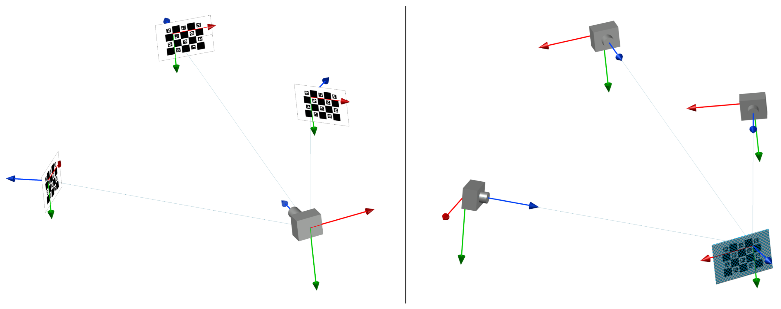
If a calibration board printed on a sheet of paper is used, the camera is typically fixed, and the board changes its orientation with respect to the camera across successive images. In contrast, when the calibration experiment requires displaying the board on a projector screen, monitor, or television display, successive calibration images must be acquired by changing the pose of the camera (Figure 1).

This naturally leads to the question of whether camera calibration using a board displayed on a screen is equivalent to calibration using a printed board. A related question is what it means for two calibration procedures to be considered equivalent.

We adopt a natural criterion: a small difference in projection errors obtained from the same set of images will be taken as evidence of equivalence between the calibration models.

This, however, raises a new issue: can we ensure the same set of identical images in both acquisition modes? Below, we argue that a simple exchange of the camera and board poses, followed by the application of an appropriately chosen isometry—consisting of a rotation and a translation—yields the same image.

What does a simple exchange mean in this context? Suppose that, in some reference coordinate system, the calibration board has pose $(U,u)$ and the camera has pose $(V,v)$. Since the camera observes the board, and the board has its z-axis aligned with the viewing direction, exchanging their roles requires not only swapping positions but also reversing the directions of the z- and x-axes. The reversal of the x-axis is necessary to preserve a right-handed coordinate system. This transformation is achieved by multiplying the pose components by the orthonormal matrix

$$E_{xz}=\left[\begin{array}{ccc}-1& 0& 0\\ 0& 1& 0\\ 0& 0& -1\end{array}\right]⟹U^{\prime }\doteq E_{xz}U,u^{\prime }\doteq E_{xz}u,V^{\prime }\doteq E_{xz}V,v^{\prime }\doteq E_{xz}v.$$

After this operation, the camera pose becomes $(U^{\prime },u^{\prime })$, while the board pose becomes $(V^{\prime },v^{\prime })$.

Theorem 2

(On corrective isometry under exchange of camera and board poses). The corrective isometry is defined by the rotation matrix $W={\left(R_{vu}\right)}^2$ and the translation vector $w=(I_3-R_{vu})t_{vu}$, where the isometry $(R_{vu},t_{vu})$ represents the transformation from the board coordinate system to the camera coordinate system. Under this transformation, the original image is identical to the image obtained after exchanging the camera and board poses and applying the corrective isometry.

Proof. 

Let a point P have coordinates x in the board coordinate system $(U,u)$. Its coordinates in the reference frame are then $y=Ux+u$, and consequently its coordinates in the camera coordinate system $(V,v)$ are given by

$$y_v=V^{⊺}(y-v).$$

Substituting y, we obtain

$$y_v=V^{⊺}(Ux+u-v)=\underset{\doteq R_{vu}}{\underbrace{V^{⊺}U}}x+\underset{\doteq t_{vu}}{\underbrace{V^{⊺}(u-v)}}=R_{vu}x+t_{vu}.$$

After exchanging the poses and applying the sign changes to the x- and z-axes, we use the same expression to compute the transformation from the new board coordinate system $(V^{\prime },v^{\prime })$, where $V^{\prime }\doteq E_{xz}V$ and $v^{\prime }\doteq E_{xz}v$, to the new camera coordinate system $(U^{\prime },u^{\prime })$, where $U^{\prime }\doteq E_{xz}U$ and $u^{\prime }\doteq E_{xz}u$:

$$y_u={\left(U^{\prime }\right)}^{⊺}(V^{\prime }x+v^{\prime }-u^{\prime })=U^{⊺}\underset{=I_3}{\underbrace{E_{xz}^{⊺}{E}_{xz}}}Vx+U^{⊺}\underset{=I_3}{\underbrace{E_{xz}^{⊺}{E}_{xz}}}(v-u)=U^{⊺}Vx+U^{⊺}(v-u).$$

Since, in general, $y_u\ne y_v$, the same image is not obtained directly. We therefore seek an isometry such that $y_v=W{y}_u+w$ for all $x\in {\mathbb{R}}^3$:

$$\left(V^{⊺}U\right)x+V^{⊺}(v-u)=W(U^{⊺}Vx+U^{⊺}(u-v))+w.$$

From this equation we obtain

$$W{U}^{⊺}V=V^{⊺}U⟹W={\left(V^{⊺}U\right)}^2=R_{vu}^2,$$

and

$$w=V^{⊺}(u-v)-W{U}^{⊺}(u-v)⟹w=t_{vu}-\underset{=V^{⊺}U\doteq R_{vu}}{\underbrace{W{U}^{⊺}V}}{t}_{vu}=(I_3-R_{vu})t_{vu}.$$

□

The presented duality does not introduce a new calibration model but rather illustrates the geometric equivalence of different experimental configurations. This observation is particularly relevant in the context of calibration using emissive displays such as OLED panels.

In the remainder of the paper, the camera pose estimation problem is addressed using a rotation parameterization in Cayley space. For completeness and notational clarity, we briefly recall the definition of the Cayley rotation matrix and its properties, which are used both in the theoretical analysis and in the description of the PnP-ProCay78 algorithm. A more complete, yet concise, summary of the Cayley representation is provided in Appendix A.

4.3. Cayley Representation of Rotations

For completeness and notational clarity, we recall the definition of the Cayley rotation matrix and its basic properties, restricting the presentation to the forms used directly in the remainder of the paper. A more detailed discussion of the Cayley representation can be found in Appendix A.

Matrix form

Let $v\in {\mathbb{R}}^3$. The Cayley rotation matrix $R\left(v\right)\doteq R^{+1}\left(v\right)$ and its inverse $R^{-1}\left(v\right)=R^{\top }\left(v\right)=R(-v)$ share the following compact matrix representation, using the paired signs $\pm ,\mp$:

$$R^{\pm }={\mathbf{I}}_3\pm {\displaystyle \frac{2·\widehat{v}·({\mathbf{I}}_3\pm \widehat{v})}{1+{\parallel v\parallel }^2}},$$

where $\widehat{v}$ denotes the skew-symmetric matrix associated with the vector v, satisfying the standard properties of such matrices (see Appendix A).

Element-wise form

Let $v\in {\mathbb{R}}^3$. The Cayley rotation matrix $R\left(v\right)\doteq R^{+1}\left(v\right)$ and its inverse $R^{-1}\left(v\right)=R^{\top }\left(v\right)=R(-v)$ admit the following explicit representation, again using the paired signs $\pm ,\mp$:

$$R^{\pm }={\displaystyle \frac{1}{1+v_x^2+v_y^2+v_z^2}}\left[\begin{array}{ccc}1+v_x^2-v_y^2-v_z^2& 2(v_x{v}_y\mp v_z)& 2(v_x{v}_z\pm v_y)\\ 2(v_x{v}_y\pm v_z)& 1+v_y^2-v_x^2-v_z^2& 2(v_y{v}_z\mp v_x)\\ 2(v_x{v}_z\mp v_y)& 2(v_y{v}_z\pm v_x)& 1+v_z^2-v_x^2-v_y^2\end{array}\right].$$

The paired signs ± and ∓ correspond respectively to the rotation matrix and its inverse. This property and its geometric consequences are discussed in more detail in Appendix A.

5. Initial Estimation of the Calibration Board Pose

5.1. Experimental Data

In this subsection, we describe the experimental dataset used for the initial identification of the calibration board position and orientation with respect to the camera, as well as for evaluating the behavior of the considered PnP algorithms. Particular emphasis is placed on the heterogeneity of the data, encompassing both high-resolution RGB vision cameras and thermal cameras with resolutions on the order of several tens of pixels. Such a configuration allows not only for assessing the accuracy of the methods under strongly varying data quality conditions, but also for analyzing their stability and convergence properties in the context of sensors with extremely different geometric and photometric characteristics.

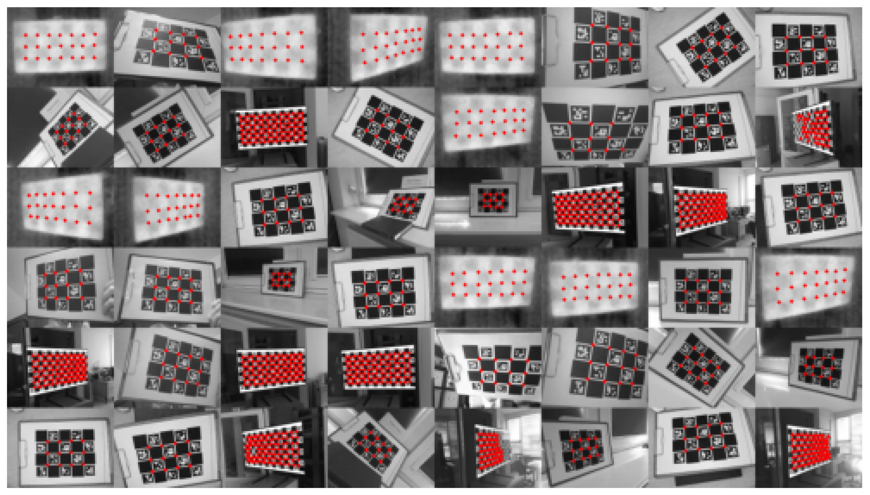
To illustrate the diversity and heterogeneity of the calibration data used in this study, a representative mosaic of calibration images is shown in Figure 2. The dataset comprises images acquired using multiple camera modalities, including high-resolution RGB sensors and low-resolution thermal cameras, resulting in a wide range of spatial resolutions, noise characteristics, and photometric properties.

Each tile in the mosaic corresponds to an individual calibration image, uniformly rescaled to a common display resolution for visualization purposes. Prior to geometric rescaling, all images undergo an achromatic preprocessing step, in which per-pixel chromatic information is suppressed by projecting RGB values onto a single luminance channel. Specifically, the maximum value across color channels is replicated to all channels, yielding a strictly achromatic representation. This operation eliminates chromatic interpolation artifacts that may arise during resolution reduction, particularly for images acquired from OLED displays under low-light conditions.

Detected corner locations are overlaid after the mosaic assembly in a common coordinate frame, ensuring resolution-independent visualization and preventing the disappearance of corner markers in low-resolution imagery. This separation of geometric rescaling and feature overlay guarantees consistent marker visibility across different sensor modalities.

An optional random permutation of tiles is employed solely for visualization purposes, avoiding any implicit ordering bias while preserving full reproducibility.

The dataset prepared in this manner serves as a common basis for all subsequent comparative experiments. The same calibration images are used both for analyzing the properties of the matrix $\Omega$, for selecting the initial points of the PnP-ProCay78 algorithm, and for comparisons with reference algorithms available in the OpenCV library.

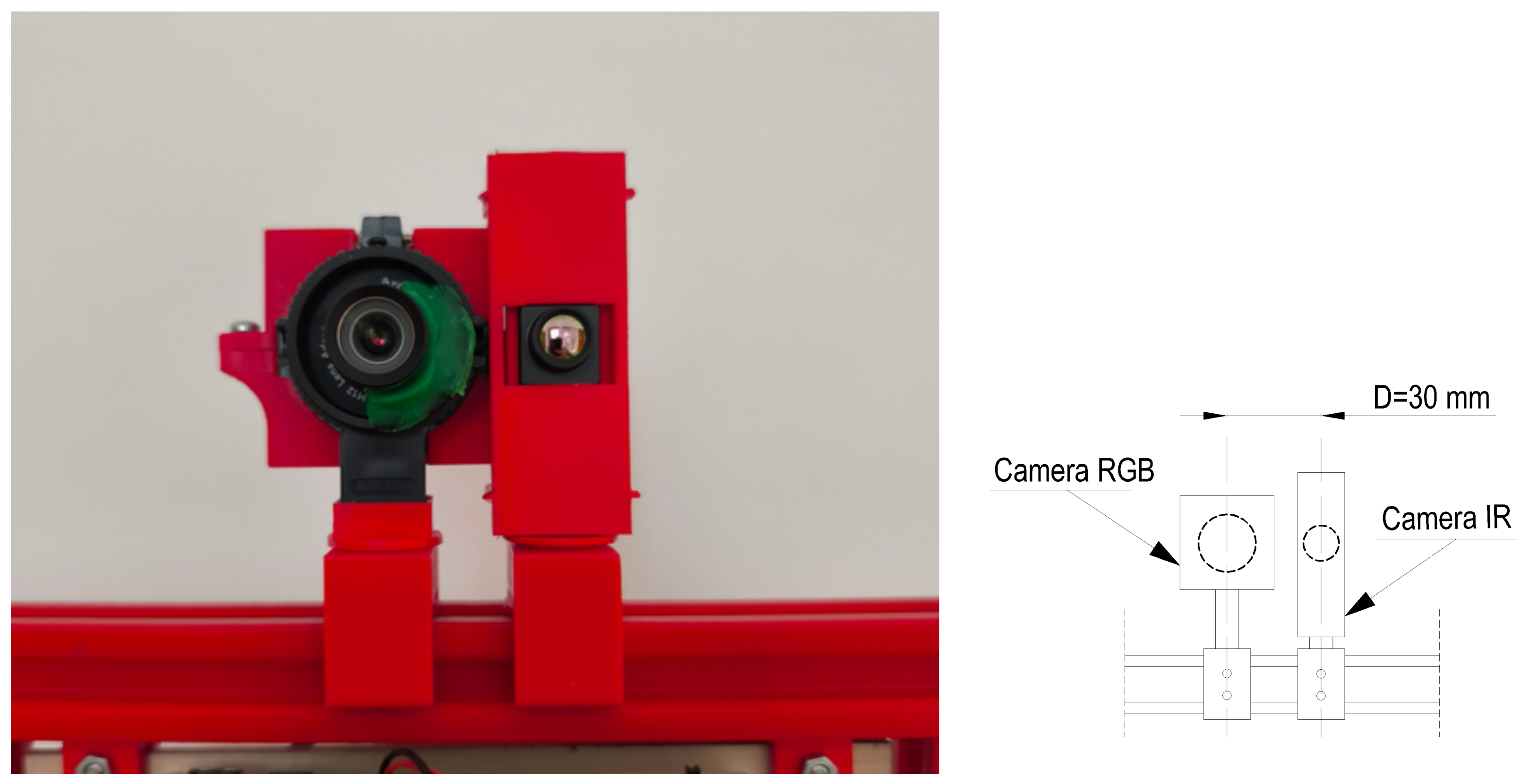
Figure 3 shows the physical configuration of the RGB and IR camera setup used in the experiments. On the left, the complete set of sensors mounted on the RP5 (Raspberry Pi 5) computing platform is presented, comprising a high-resolution RGB camera and a low-resolution thermal camera. A technical sketch of the lens layout for these cameras is shown on the right. The sketch shows that the optical center distance is approximately 30 mm. A small geometric baseline between the cameras facilitates synchronous analysis of the optimization trajectories for RGB and IR data while maintaining comparable observation geometry.

The experimental dataset defined in this way, comprising both high-quality RGB images and spatially highly degraded thermal images, constitutes a challenging test environment for camera pose estimation algorithms. In particular, it enables an assessment of how the algebraic properties of the matrix $\Omega$ and the choice of initialization points influence the stability and convergence of optimization procedures under conditions of significant differences in image resolution and point localization accuracy. In the following subsection, the described data are used to introduce and discuss in detail the PnP-ProCay78 algorithm, whose construction was directly inspired by observations made on this experimental dataset.

5.2. The PnP-ProCay78 Algorithm

The stage of initial estimation of the calibration object pose, that is, its position and orientation with respect to the camera coordinate system, is crucial not only for accurate pose identification but also for the subsequent estimation of camera parameters, including the distortion model and the sensor plane geometry.

Within the OpenCV framework, several methods for initial pose estimation are provided. Among them, the technique based on the SQPnP algorithm proposed by Terzakis et al. [4] is distinguished by its direct minimization of the quadratic reconstruction error ${\mathcal{E}}^2\doteq r^{\top }\Omega r$ (see Equations (1)–(4)). The algorithm searches for an optimal solution on the sphere $\mathbb{S}({\mathbf{0}}_9;\sqrt{3})$, starting from selected saddle points. These points are first projected onto the nearest points on the sphere representing valid rotations, after which a constrained quadratic programming procedure is applied. In a small number of iterations, this process yields a candidate for an optimal rotation.

A candidate saddle point is discarded if the reconstruction error of its nearest rotation exceeds the smallest error found so far. Importantly, saddle points are located in regions of local convexity of the cost function under rotational constraints, which guarantees the existence of a local minimum in such regions, although not necessarily the global one. Consequently, these regions must be systematically explored. For planar scenes, the kernel of the matrix $\Omega$ has dimension four, and each nonzero eigenvalue of $\Omega$ defines two symmetric saddle points on the sphere centered at the origin. This leads to at most $2·(9-4)=10$ candidate regions to be examined.

Although SQPnP is currently regarded as one of the most effective solvers for the PnP problem, its construction does not explicitly exploit information arising from the special structure of calibration scenes. In particular, for planar scenes, the properties of the matrix $\Omega$ suggest the possibility of a more directed and deterministic selection of starting points.

Our attempt at refining an already optimal solution is therefore based on the following observations regarding the SQPnP technique:

• The algorithm is designed for both 2D and 3D calibration scenes and thus cannot exploit the specific structure of the quadratic form $r^{\top }\Omega r$ induced by the assumption $Z_i=0$ for points expressed in the local coordinate system of a planar calibration board. In particular, for planar scenes, the canonical basis vectors $e_3,e_6,e_9$ belong to the kernel of $\Omega$ (see Theorem 1).
• The reconstruction error values at saddle points, equal to the eigenvalues of $\Omega$, are either zero (${\lambda }_1=\dots ={\lambda }_4=0$) or equal to one (${\lambda }_7=\dots ={\lambda }_9$) in the planar case. The eigenvalues ${\lambda }_5$ and ${\lambda }_6$ lie very close to the kernel, suggesting that the search should be initiated precisely from the corresponding directions. This behavior, however, is not reflected in the SQPnP pseudocode.
• The optimization iterations have a Newton-like character but are performed in an extended state vector of dimension $n=9+6=15$. In contrast, the Cayley representation reduces the number of independent parameters to $n=3$. Although the Hessian matrix is approximated by the outer product of the Jacobian, which depends on the number of calibration points, this does not significantly increase the computational cost, especially for low-resolution images such as those encountered in thermal imaging.

These observations motivated the following strategy:

1.

Optimization is performed in the Cayley representation of rotations using a generic nonlinear least-squares solver, either Trust Region Reflective (TRF) or Levenberg-Marquardt (LM) [18].

2.

The initial iteration point is selected based on the smallest positive value of the cost function $\mathcal{E}(e_i;P,p)$ evaluated at the canonical basis vectors $[e_1,\dots ,e_9]\equiv I_9$. Specifically, the vector $\sqrt{3}{e}_{i_{min}}$ determines the initial Cayley vector $v_1^{\left(\mathrm{start}\right)}$.

3.

The second initial vector is chosen as the antipodal Cayley vector corresponding to the opposite rotation: $v_2^{\left(\mathrm{start}\right)}\doteq -v_1^{\left(\mathrm{start}\right)}$.

4.

The solution of the lsq optimization yielding the smaller reconstruction error is selected as the final PnP solution.

Note that eigenvalue analysis is not used in our approach to optimizing the quadratic reconstruction function $\mathcal{E}(r;P,p)$ represented by the quadratic form of the matrix $\Omega$. The SQPnP algorithm considers the eigenvector basis as the starting points, while ProCay78 uses the canonical basis to achieve this goal.

In the following subsections, we demonstrate the consequences of selecting $v_{\mathrm{start}}$ based on canonical basis vectors and present the final form of the algorithm, which we name PnP-ProCay78 after Procrustes, Cayley, and the indices 7 and 8 of the selected canonical vectors.

5.2.1. How Are the Initial Cayley Vectors Selected?

To determine which canonical vectors should be chosen, we analyze the frequency statistics of minimal-cost occurrences and the average cost values associated with individual canonical directions (

Table 2. Histogram of canonical vector indices corresponding to the minimum positive reconstruction error. The mean error value is also reported for each canonical vector group.

Camera Name	Number of Photos	Histogram at Minimum (%)	Error Means for Canonical Groups
RP5-RGB (2048 × 1520)	31	$0_{1-6},{42}_7,{58}_8,0_9$	$0_{3,6,9},0.{00049}_{8,7},0.{51}_{5,1},0.{99}_{4,2}$
RP5-IR (80 × 62)	22	$0_{1-6},{32}_7,{68}_8,0_9$	$0_{3,6,9},0.{0032}_{8,7},0.{51}_{5,1},0.{99}_{4,2}$
PC-Aver (640 × 480)	12	$0_{1-6},{58}_7,{42}_8,0_9$	$0_{3,6,9},0.{0057}_{7,8},0.{53}_{1,5},0.{97}_{4,2}$
PC-Logitex (640 × 480)	7	$0_{1-6},{43}_7,{57}_8,0_9$	$0_{3,6,9},0.{0035}_{8,7},0.{58}_{5,1},0.{92}_{4,2}$
PC-USB (640 × 480)	8	$0_{1-6},{50}_7,{50}_8,0_9$	$0_{3,6,9},0.{0067}_{7,8},0.{50}_{1,5},0.{99}_{4,2}$

). These statistics are computed from several dozen calibration images acquired during the calibration of five different cameras. Representative raw data used to compute these statistics are provided in Appendix C for experiments involving RGB and IR cameras mounted on the RP5 (Raspberry Pi 5) computing platform.

Table 2 leads to an unambiguous conclusion: for every calibration image, the smallest positive reconstruction error is attained either for the canonical vector $e_7$ or for $e_8$.

This observation allows the initial Cayley vectors $v_7$ and $v_8$ to be determined independently of the specific input data used by the PnP-ProCay78 algorithm.

The computation follows the scheme

$$\sqrt{3}{e}_i\stackrel{\mathrm{vector} \mathrm{to} \mathrm{matrix}}{\to }{E}_i\stackrel{{\mathrm{Procrustes}}^{+}}{\to }{R}_i\stackrel{\mathrm{Cayley}}{\to }{v}_i.$$

Details of the Procrustes procedure and its modification used in this work are provided in Appendix B.

Table 3. Cayley representations of the nearest rotation matrices and their antipodes computed for the selected canonical points $\sqrt{3}{e}_i$ on the search sphere $S({\mathbf{0}}_9;\sqrt{3})$ in the Euclidean space ${\mathbb{R}}^9$, for $i=7,8,9$.

$\sqrt{3}{e}_i$	matrix $E_i$	nearest $R_i$	Cayley $v_i$	antipodal ${\overline{R}}_i$	Cayley ${\overline{v}}_i$
$\sqrt{3}{e}_7$	$\left[\begin{array}{ccc}0& 0& 0\\ 0& 0& 0\\ \sqrt{3}& 0& 0\end{array}\right]$	$\left[\begin{array}{ccc}0& 0& -1\\ 0& 1& 0\\ 1& 0& 0\end{array}\right]$	$\left[\begin{array}{c}0\\ -1\\ 0\end{array}\right]$	$\left[\begin{array}{ccc}0& 0& 1\\ 0& 1& 0\\ -1& 0& 0\end{array}\right]$	$\left[\begin{array}{c}0\\ 1\\ 0\end{array}\right]$
$\sqrt{3}{e}_8$	$\left[\begin{array}{ccc}0& 0& 0\\ 0& 0& 0\\ 0& \sqrt{3}& 0\end{array}\right]$	$\left[\begin{array}{ccc}1& 0& 0\\ 0& 0& -1\\ 0& 1& 0\end{array}\right]$	$\left[\begin{array}{c}1\\ 0\\ 0\end{array}\right]$	$\left[\begin{array}{ccc}1& 0& 0\\ 0& 0& 1\\ 0& -1& 0\end{array}\right]$	$\left[\begin{array}{c}-1\\ 0\\ 0\end{array}\right]$
$\sqrt{3}{e}_9$	$\left[\begin{array}{ccc}0& 0& 0\\ 0& 0& 0\\ 0& 0& \sqrt{3}\end{array}\right]$	$\left[\begin{array}{ccc}1& 0& 0\\ 0& 1& 0\\ 0& 0& 1\end{array}\right]$	$\left[\begin{array}{c}0\\ 0\\ 0\end{array}\right]$	$\left[\begin{array}{ccc}1& 0& 0\\ 0& -1& 0\\ 0& 0& -1\end{array}\right]$	$\begin{array}{c}Undefinedas\\ tr\overline{R}=-1\end{array}$

lists the results of these computations for $e_7$ and $e_8$. For completeness, the case of $e_9$ is also included. Its nearest rotation is the identity matrix $I_3$, corresponding to a zero Cayley vector. The antipodal matrix $-I_3$ has trace equal to $-1$ and therefore does not admit a Cayley representation.

From Table 3, the two initial vectors required for the two least-squares optimizations are determined as follows:

• if $e_7^{\top }\Omega e_7<e_8^{\top }\Omega e_8$, the starting Cayley vectors are $v_7={[0,-1,0]}^{\top }$ and ${\overline{v}}_7={[0,1,0]}^{\top }$;
• otherwise, the pair $v_8={[1,0,0]}^{\top }$ and ${\overline{v}}_8={[-1,0,0]}^{\top }$ is used.

Two independent optimization runs starting from antipodal regions of the search sphere are necessary due to the symmetry of the cost function: $r^{\top }\Omega r={(-r)}^{\top }\Omega (-r)$. Starting from $R_7$, for example, the opposite point $-R_7$ yields the same cost value. Since negating a rotation matrix changes its determinant to $-1$, an Umeyama correction [19] is required:

$$\begin{array}{c}{E}_i=\mathrm{mat}\left(\sqrt{3}{e}_i\right)\stackrel{\mathrm{Procrustes}}{\to }R=[u_1,u_2,u_3]V^{\top }\stackrel{\mathrm{point} \mathrm{symmetry}}{\to }\hfill \\ -R=[-u_1,-u_2,-u_3]V^{\top }\stackrel{\mathrm{Umeyama} \mathrm{correction}}{\to }\overline{R}=[-u_1,-u_2,u_3]V^{\top }.\hfill \end{array}$$

This extension of the Procrustes procedure with the Umeyama correction is referred to as Procrustes⁺. A formal proof of its correctness and an analysis of solution uniqueness are provided in Appendix B.

Finally, we note the following:

1.

The Umeyama correction is typically applied when the Procrustes solution $R=U{V}^{\top }$ has a negative determinant. In our case, all matrices $R_i=\mathrm{Procrustes}\left(\mathrm{mat}\left(\sqrt{3}{e}_i\right)\right)$, $i=1,\dots ,9$, have determinant $+1$, whereas their antipodes have determinant $-1$, and the correction is applied only to the latter.

2.

In general, an antipodal rotation does not correspond to the negation of the Cayley vector, since $R_{-v}=R_v^{\top }\ne -R_v$. However, for the specific cases of $R_7$ and $R_8$ listed in Table 3, this equality holds.

3.

The starting points in SQPnP are scaled eigenvectors of $\Omega$ and thus depend on all matrix entries. In contrast, the starting points of PnP-ProCay78 depend solely on the comparison of the diagonal elements ${\Omega }_{77}$ and ${\Omega }_{88}$:

$$\begin{array}{c}{\Omega }_{77}<{\Omega }_{88}⟹\left\{\left[\begin{array}{c}0\\ -1\\ 0\end{array}\right],\left[\begin{array}{c}0\\ 1\\ 0\end{array}\right]\right\},\hfill \\ {\Omega }_{77}\ge {\Omega }_{88}⟹\left\{\left[\begin{array}{c}1\\ 0\\ 0\end{array}\right],\left[\begin{array}{c}-1\\ 0\\ 0\end{array}\right]\right\}.\hfill \end{array}$$

5.2.2. The PnP-ProCay78 Algorithm: Pseudocode

The pseudocode for the ProCay78 algorithm consists of two parts:

1.

Algorithm 1, which prepares starting points and calls two optimization paths.

2.

Algorithm 2, which is called by the optimizer when it wants to obtain a vector of residual values. A pair of points $(P_i,p_i)$, i.e., a calibration point on the board and its corresponding point on the viewport, contributes two values $xy$ to this vector.

$${\left({\displaystyle \frac{(R{P}_i+t)}{{(R{P}_i+t)}_z}}\right)}_x-{\left(p_i\right)}_x,{\left({\displaystyle \frac{(R{P}_i+t)}{{(R{P}_i+t)}_z}}\right)}_y-{\left(p_i\right)}_y$$

Comments on Singularity of Cayley Representation

• Let us first note that the algorithm ProCay78 always starts optimization with a Cayley vector of unit norm and represents a rotation matrix with trace equal to 1 (see Table 3). The LSM optimizer generates a finite number of updates to the state vector; therefore, during optimization the norm of the Cayley vector remains bounded and safely away from infinity. From the formula $\parallel v\parallel =tan(\alpha /2)$, we see that only very large Cayley vectors can approximate rotations by $\pi$.
• On the other hand, we use PnP algorithms in our research as part of the calibration process at the stage of initializing the extrinsic parameters. We determine the axes of the board frame in the camera frame, which define the rotation matrix of the camera frame with respect to the board frame. If the trace of this matrix were $-1$, the rotation would correspond to $\pi$ about some axis. In such a case, the camera z-axis would move to the board $-z$-axis; however, by assumption these axes form an angle smaller than $\pi /2$. This contradiction implies that the pose matrix in the calibration setting cannot have a trace equal to $-1$, and the acute-angle condition ensures that its trace remains safely distant from $-1$. Moreover, the Cayley vector of the camera pose should lie within a sphere of radius 1.

It is worth emphasizing that the proposed PnP-ProCay78 algorithm employs a hybrid use of cost functions that play complementary roles in the estimation process. Like in the SQPnP algorithm, the translation vector t is eliminated analytically by enforcing the stationarity condition of the reconstruction error with respect to t, which leads to a closed-form linear operator $\mathcal{T}$ mapping the rotation matrix R to the corresponding optimal translation. In contrast, the nonlinear optimization stage (TRF or LM) operates directly on projection residuals, which constitute the primary application-level metric of pose accuracy.

Although the final optimization stage minimizes projection residuals, the translation component is obtained analytically by enforcing stationarity of the quadratic reconstruction error with respect to translation. This hybrid design separates metric alignment from optimization efficiency.

The PnP-ProCay78 algorithm and the ReconstructionResidual function (required by the LSM optimizer).

Algorithm 1 PnP-ProCay78

$\begin{array}{cc}\mathbf{Input:}\hfill & \left\{\begin{array}{l}P\in {\mathbb{R}}^{n\times 3}—\mathrm{board} \mathrm{points} \mathrm{with} P_{:,z}={\mathbf{0}}_n,\\ p\in {\mathbb{R}}^{n\times 3}—\mathrm{image} \mathrm{points} \mathrm{with} p_{:,z}={\mathbf{1}}_n,\\ \Omega —\mathrm{reconstruction} \mathrm{error} \mathrm{matrix},\\ \mathcal{T}—\mathrm{translation} \mathrm{operator}.\end{array}\right.\end{array}$ Output: $(R,t)$ with minimal reconstruction error. 1: $\begin{array}{cc}{v}_{\mathrm{start}}\leftarrow \hfill & \left\{\begin{array}{ll}{[0,-1,0]}^{\top },\hfill & \mathbf{if}{\Omega }_{77}<{\Omega }_{88},\hfill \\ {[1,0,0]}^{\top },& \mathbf{otherwise}.\end{array}\right.\hfill \end{array}$ 2: $(v,\gamma )\leftarrow LS{M}_{trf}(RR,v_{\mathrm{start}};P,p,\mathcal{T})$ 3: $(\overline{v},\overline{\gamma })\leftarrow LS{M}_{trf}(RR,-v_{\mathrm{start}};P,p,\mathcal{T})$ (* LSMtrf denotes the trf-based least-squares solver returning a Cayley vector and its associated loss value *) 4: if $\overline{\gamma }>\gamma$ then $v^{\ast }\leftarrow v$ else $v^{\ast }\leftarrow \overline{v}$ 5: $R\leftarrow CayleyToMatrix\left(v^{\ast }\right)$ 6: $t\leftarrow \mathcal{T}\mathrm{vec}\left(R\right)$ 7: return $(R,t)$

Algorithm 2 RR (Reconstruction Residuals)

$\begin{array}{cc}\mathbf{Input:}\hfill & \left\{\begin{array}{c}v—\mathrm{current} \mathrm{Cayley} \mathrm{vector},\hfill \\ P,p,\mathcal{T}—\mathrm{as} \mathrm{in} \mathtt{PnP}\mathtt{\text{-}}\mathtt{ProCay}\mathtt{78}\end{array}\right.\hfill \end{array}$ Output: $e_{\mathrm{vec}}$ — residual error vector. 1: R ← CayleyToMatrix(v) 2: $t\leftarrow \mathcal{T}\mathrm{vec}\left(R\right)$ 3: $Q\leftarrow P{R}^{\top }+t$ 4: $E\leftarrow {(Q\oslash Q_{:,z}-p)}_{:,xy}$ (* Elementwise operations are broadcasted *) 5: $e_{\mathrm{vec}}\leftarrow \mathrm{vec}\left(E\right)$ 6: return $e_{\mathrm{vec}}$

This separation mirrors a common design pattern observed in modern optimization and learning-based methods [20], where a surrogate objective is used to structure the model efficiently, while the final optimization is driven by the target performance metric. In this sense, PnP-ProCay78 can be interpreted as a geometrically motivated hybrid approach that combines an analytically tractable surrogate (reconstruction error) with a physically meaningful loss function (projection error).

5.2.3. PnP-ProCay78 Versus PnP-OpenCV: Experimental Results

In our experiments, we compared the camera pose identification results of our PnP-ProCay78 algorithm with three leading PnP algorithms included in the OpenCV library: SQPnP, IPPE, EPnP. Measurements were performed for five different cameras. Two of them, marked in the table as RP5-RGB and RP5-IR, were integrated into a Raspberry Pi 5 system. Two other cameras, marked here as PC-Logit and PC-USB, are inexpensive webcams connected to PCs. The fifth camera is a slightly more expensive laboratory system used primarily by lecturers for remote handwriting image transmission.

Table 4. Comparison of error statistics (RMSE, median, max) for four PnP methods and five cameras. For each camera, in addition to the projection error computed in the camera projective plane, the reprojection error in pixels is also estimated. For this purpose, a preliminary estimation of the focal length in pixels is used (see column $f_{\mathrm{pixel}}$). All values in the table are normalized by the coefficient $scale$ (see column $scale$), i.e., $true\_value=value·scale$. For PnP-ProCay78 algorithm the TRF was used. However, for LM optimizer the results are nearly the same.

Camera		ProCay78	SQPnP [4]	IPPE [15]	EPnP [11]
(fpixel)	Scale	(RMSE, Med, Max)	(RMSE, Med, Max)	(RMSE, Med, Max)	(RMSE, Med, Max)
RP5-RGB	${10}^{-4}$	$(0.35,0.24,1.03)$	$(0.35,0.24,1.02)$	$(0.35,0.24,1.03)$	$(10.33,3.38,68.21)$
$\left(2175\right)$	${10}^{-1}$	$(0.76,0.51,2.24)$	$(0.76,0.51,2.22)$	$(0.76,0.52,2.23)$	$(22.46,7.35,148.33)$
RP5-IR	${10}^{-4}$	$(10.90,6.67,28.27)$	$(10.92,6.41,29.13)$	$(11.08,6.50,29.14)$	$(111.55,53.20,347.48)$
$\left(97\right)$	${10}^{-1}$	$(1.05,0.64,2.73)$	$(1.05,0.62,2.81)$	$(1.07,0.63,2.81)$	$(10.77,5.14,33.56)$
PC-Logitex	${10}^{-4}$	$(1.18,0.65,3.38)$	$(1.18,0.64,3.38)$	$(1.48,0.70,3.54)$	$(4.73,3.13,13.67)$
$\left(563\right)$	${10}^{-1}$	$(0.66,0.37,1.90)$	$(0.66,0.36,1.90)$	$(0.83,0.40,1.99)$	$(2.66,1.76,7.69)$
PC-Aver	${10}^{-4}$	$(1.35,0.73,4.69)$	$(1.35,0.72,4.68)$	$(1.55,0.95,4.20)$	$(4.19,1.78,20.94)$
$\left(604\right)$	${10}^{-1}$	$(0.81,0.44,2.84)$	$(0.81,0.44,2.83)$	$(0.93,0.58,2.54)$	$(2.53,1.07,12.66)$
PC-USB	${10}^{-4}$	$(2.70,2.46,5.70)$	$(2.71,2.49,5.44)$	$(2.78,2.78,5.27)$	$(14.34,8.28,33.80)$
$\left(633\right)$	${10}^{-1}$	$(1.71,1.56,3.61)$	$(1.71,1.58,3.44)$	$(1.76,1.76,3.34)$	$(9.08,5.24,21.40)$

contains for each combination (camera, PnP algorithm) the following statistics of projection (first row) and reprojection (second row) errors: RMSE (Root Mean Square Error), median absolute error, maximum absolute error.

From the table, we conclude that for each camera, the PnP-ProCay78 and SQPnP algorithms have almost the same (re)projection error statistics. The IPPE algorithm has also nearly the same statistics, as the differences remain within numerical tolerance. The EPnP algorithm is much worse than these three leading algorithms.

5.2.4. Analysis of State Trajectories in Cayley Space

Visual analysis of optimization trajectories in Cayley space allows direct observation of differences in the behavior of algorithms, as well as the impact of input data quality (RGB vs. IR) on the convergence process.

To this end, any nonzero vector $v\in {\mathbb{R}}^3,v={[v_x,v_y,v_z]}^{⊺}$ is represented by a point $v_{xy}^{\prime }\doteq (v_x/\parallel v\parallel ,v_y/\parallel v\parallel )$ lying on the unit disk and a real number $v_n\doteq {sign}^{\prime }\left(v_z\right)·\parallel v\parallel$. The zero vector R$v\doteq {\mathbf{0}}_3$ is represented by the zero vector in the plane and the number zero.

The sign’$\left(t\right)$ function used above is computed according to the settings of the sign bits in float representation, i.e., sign’$(-0.0)=-1$ and sign’$(+0.0)=+1$, which in general means that if the sign bit is set, then sign’ returns $-1$, otherwise sign’ returns $+1$.

Such a vector decomposition is called its radially circular representation. This representation has several interesting properties:

1.

It is invertible: $\parallel v\parallel =|v_n|,(v_x,v_y)=v_n·v_{xy}^{\prime },v_z={sign}^{\prime }\left(v_n\right)·\sqrt{{\parallel v\parallel }^2-v_x^2-v_y^2}$.

2.

Each point in the plane $v_z=0$ is mapped to a point on the unit circle.

3.

Any trajectory in 3D space can be observed as a trajectory in 2D space parallel to the signed norm curve of the trajectory points.

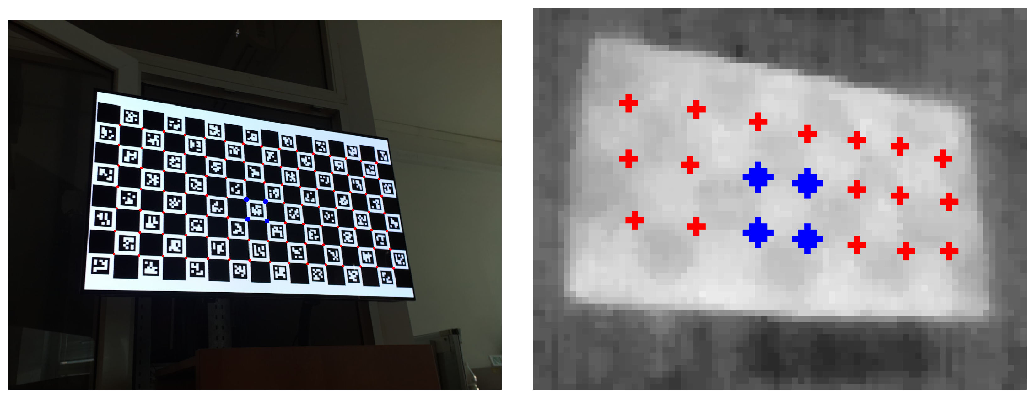
Figure 4 shows images of calibration grids displayed on an OLED screen. The image on the left was acquired by an RGB camera displaying a Charuco grid [21], while the image on the right was captured by a low-resolution thermal camera displaying a traditional, lower-resolution checkerboard. There are descriptions of thermal camera calibration using Charuco grids in scientific publications, such as [22], but in our case, detecting calibration points in an 80 × 62 resolution thermal image using Charuco tiles failed. In high-resolution images, detection of Aruco markers is effective, even under challenging lighting conditions; see [23].

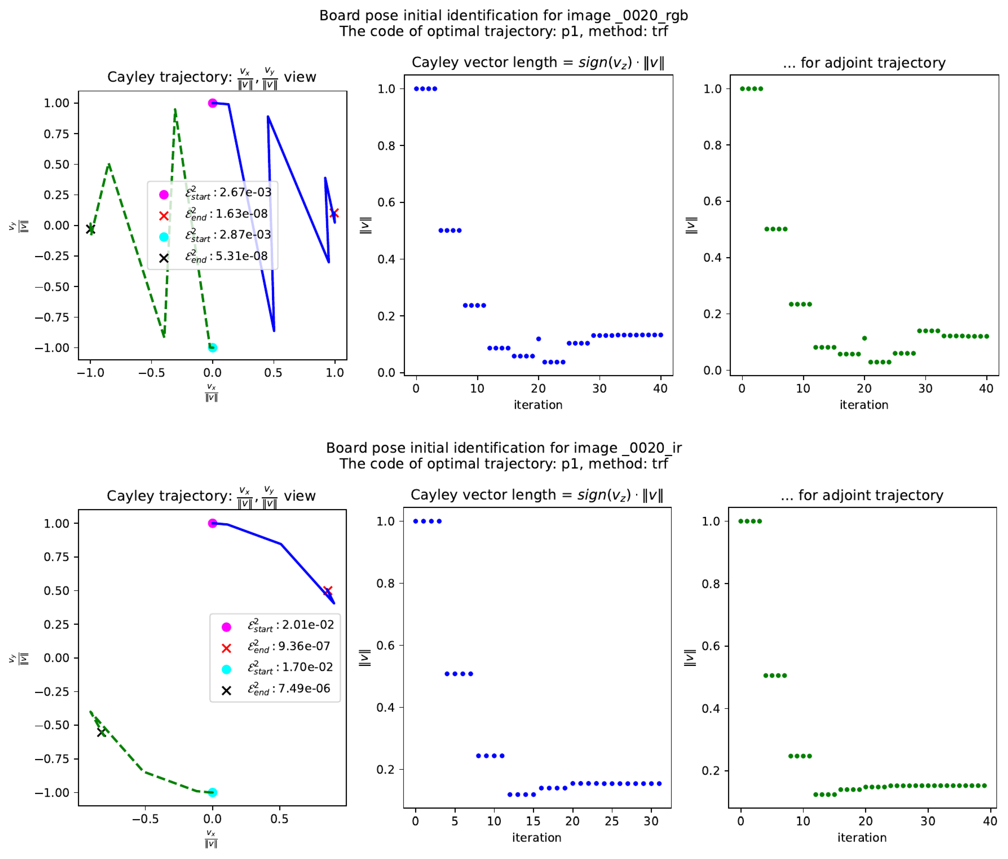
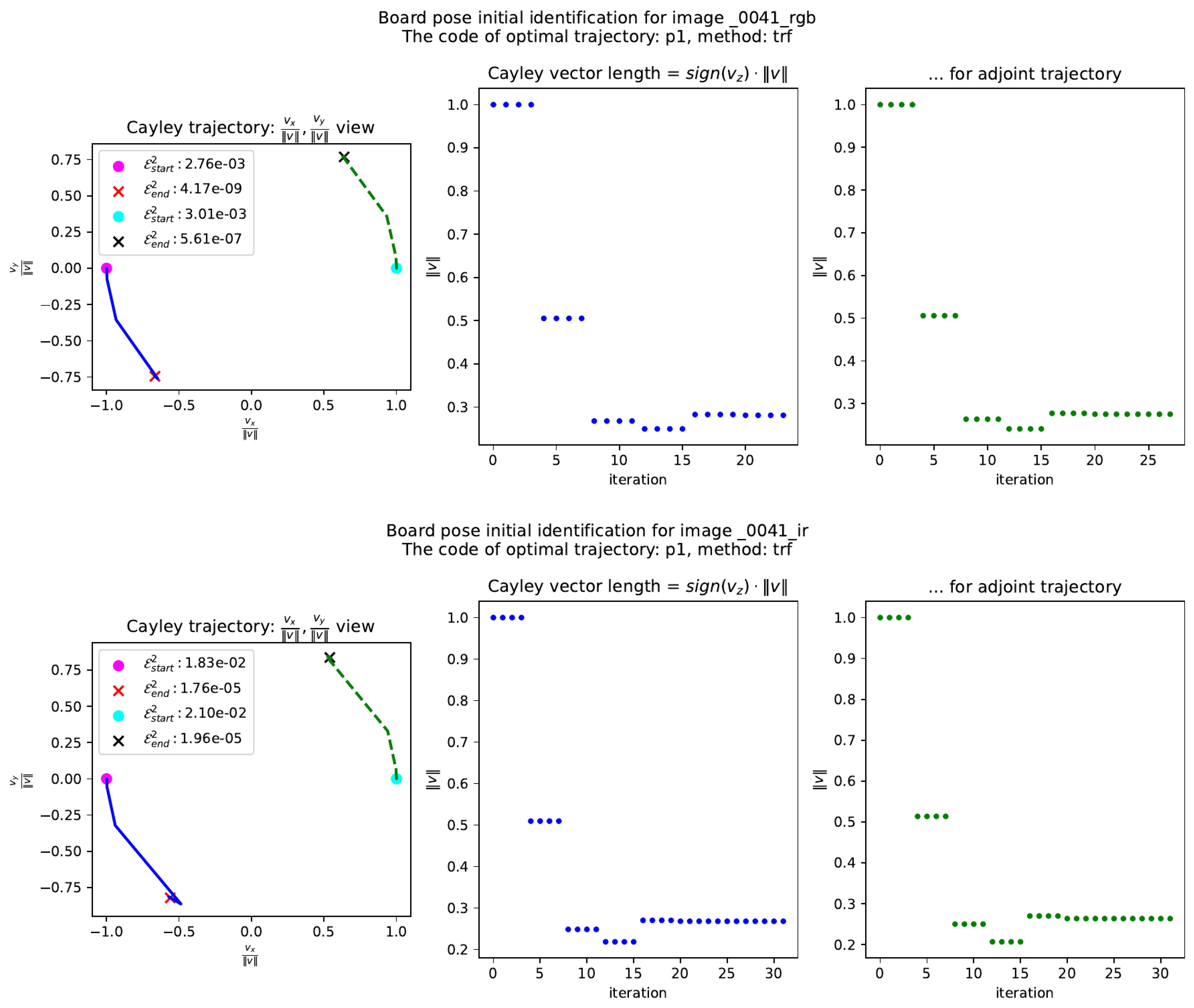
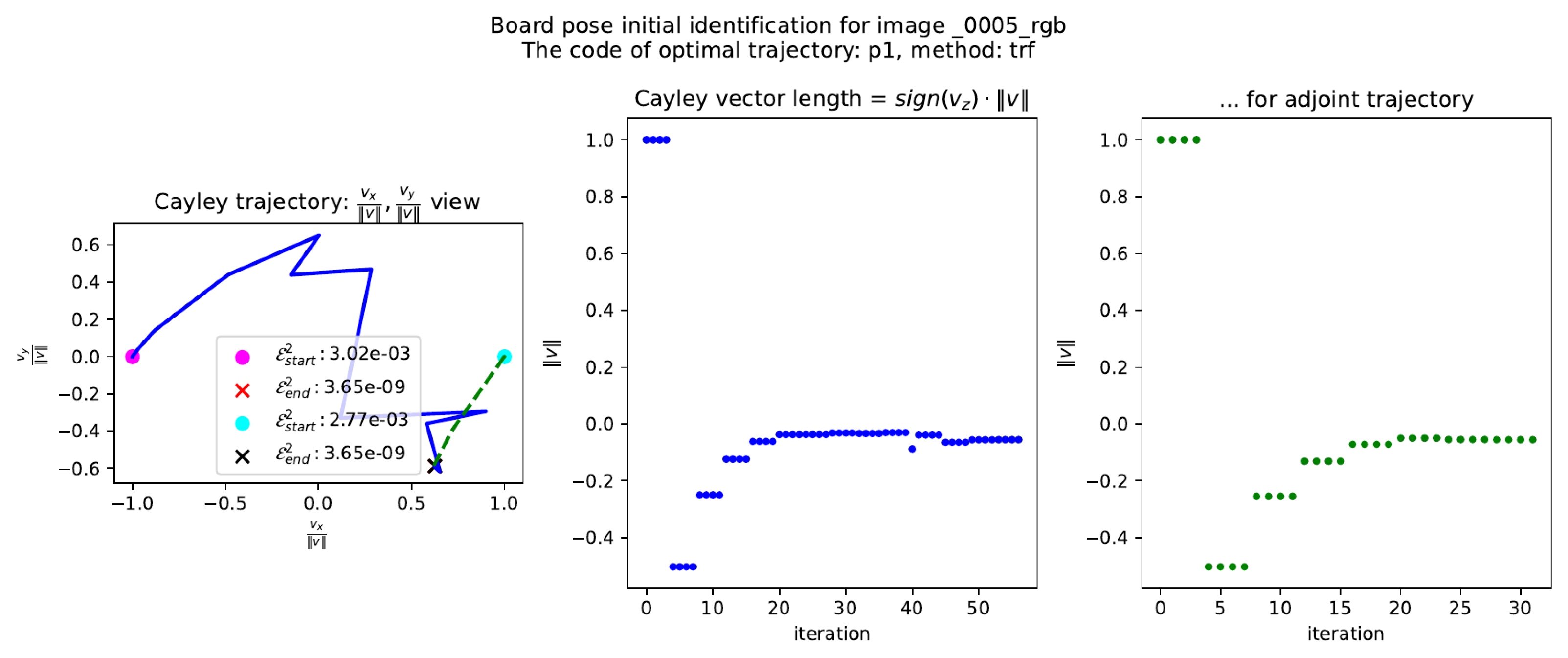
In the first row of Figure 5, we have depicted Cayley trajectories using a radial-circular visualization. The solid blue line connects the Cayley states for the iterations of the Trust Region with Reflection (TRF) algorithm, while the dashed green line represents its performance for the conjugate trajectory for states with higher projection error.

The label (code) of the trajectory indicates whether the initial Cayley vector represented the closest orthonormal matrix with a positive determinant—code p0—or with a negative determinant and the required Umeyama correction—code p1.

To the right of the trajectory within the unit disk, the signed norm values are plotted with stepwise indexing. The first step equals $v_n=1$ as the initial Cayley vectors have norms equal to one, and z coordinates zero; see Table 3. The next three points are visually the same as the specific procedural steps related to gradient computation. The final series of near-constant state norms corresponds to stabilization of the projection error. Since four Cayley evaluations are performed per effective optimizer step, convergence is typically achieved within a small number of actual state updates.

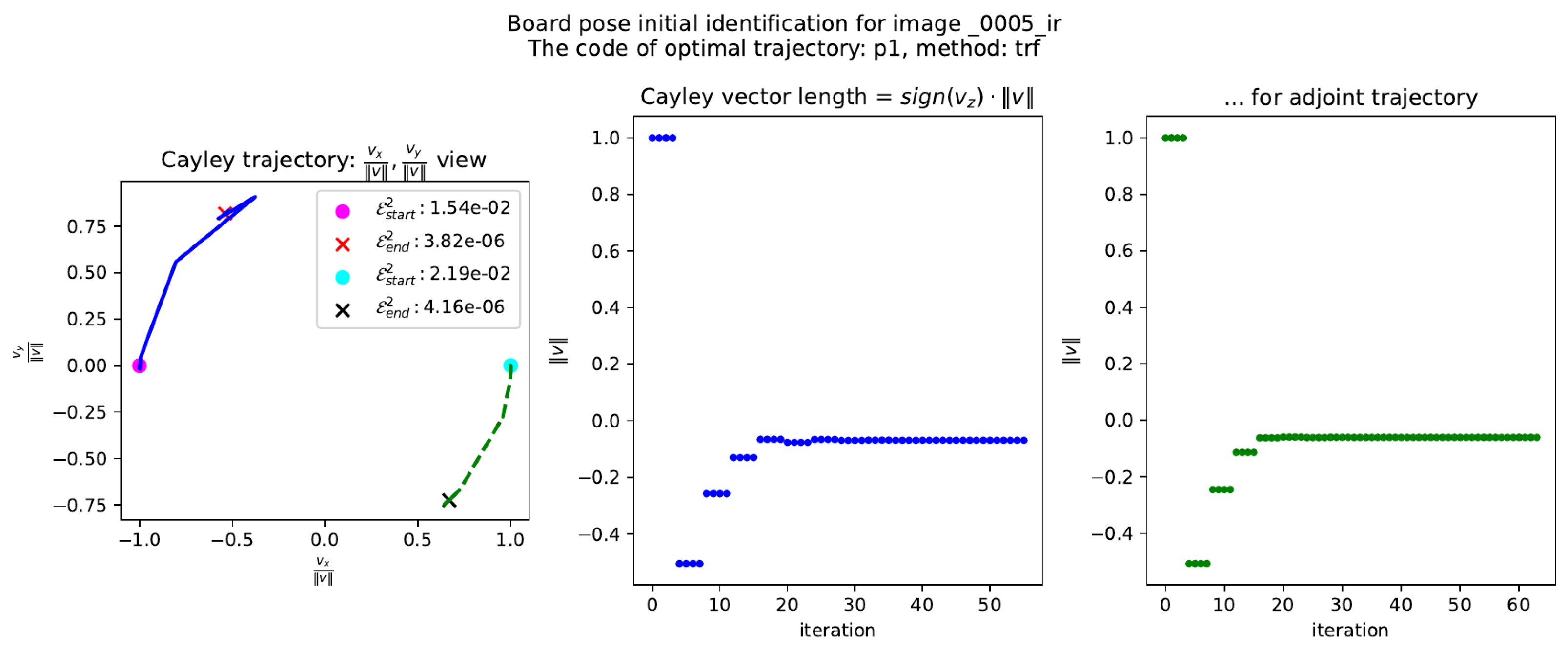
In the second row of Figure 5, we also depicted the Cayley trajectories using a radial-circular visualization for the thermal image of the same view of the board. We can observe a high visual correlation of the trajectories for identifying the positions of the visual and thermal cameras.

More experimental drawings can be found in the Appendix D.

The horizontal segments visible in the Cayley norm plots in Figure 5 correspond to four consecutive function evaluations performed at each iteration of the least-squares solver.

At a given state v, the optimizer evaluates three additional perturbed states $v+\delta e_x$, $v+\delta e_y$, and $v+\delta e_z$ in order to approximate the gradient numerically. These auxiliary evaluations are internal to the solver and do not represent actual state updates along the optimization trajectory.

Since the actual optimizer update occurs only after every four Cayley evaluations, the number of effective optimizer steps is approximately four times smaller than the number of Cayley states shown in the norm plots.

The trajectory visualizations presented above provide qualitative insight into the optimizer dynamics. In the following subsection, this analysis is complemented by a quantitative study of convergence and robustness under controlled localization noise.

5.2.5. Experimental Analysis of Convergence and Localization Noise Sensitivity

To evaluate the sensitivity of the proposed method to calibration point localization uncertainty, we performed controlled experiments in which zero-mean Gaussian noise with standard deviation $\sigma$ was added independently to the detected image points prior to pose estimation.

This procedure simulates errors introduced by corner detection inaccuracies, image blur, and limited spatial r. The experiment is designed to isolate, to a large extent, the influence of measurement noise on the optimization process.

The analysis was conducted separately for a high-resolution RGB camera (

Table 5. Robustness of ProCay78 with respect to calibration point localization noise for a high-resolution RGB camera.

$\mathit{\sigma }$ [px]	0.00	0.10	0.25	0.50	1.00	1.50	2.00
Mean error [px]	0.06	0.11	0.15	0.31	0.57	0.80	1.12
Median error [px]	0.05	0.09	0.13	0.26	0.50	0.68	0.91
RMSE [px]	0.07	0.13	0.19	0.39	0.69	0.99	1.41
Max error [px]	0.22	0.39	0.61	1.41	1.86	2.98	4.38
Mean optimizer iterations	8.73	9.24	9.33	9.18	8.71	8.93	8.76
Mean effective steps to 0.5 px	5.47	5.80	5.91	–	–	–	–
Success rate [%]	100.0	100.0	100.0	93.3	33.3	6.7	4.4

) and a low-resolution IR camera (

Table 6. Robustness of ProCay78 with respect to calibration point localization noise for a low-resolution IR camera.

$\mathit{\sigma }$ [px]	0.00	0.10	0.25	0.50	1.00	1.50	2.00
Mean error [px]	0.08	0.11	0.15	0.29	0.49	0.80	1.10
Median error [px]	0.07	0.09	0.12	0.24	0.38	0.70	0.91
RMSE [px]	0.10	0.13	0.19	0.35	0.62	0.99	1.35
Max error [px]	0.27	0.34	0.58	0.96	1.93	2.71	3.73
Mean iterations	10.40	9.84	9.42	9.56	8.53	8.38	8.11
Mean iterations to 0.5 px	3.73	3.60	3.84	3.76	–	–	–
Success rate [%]	100.0	100.0	100.0	100.0	53.3	8.9	6.7

), in order to assess robustness under substantially different noise regimes.

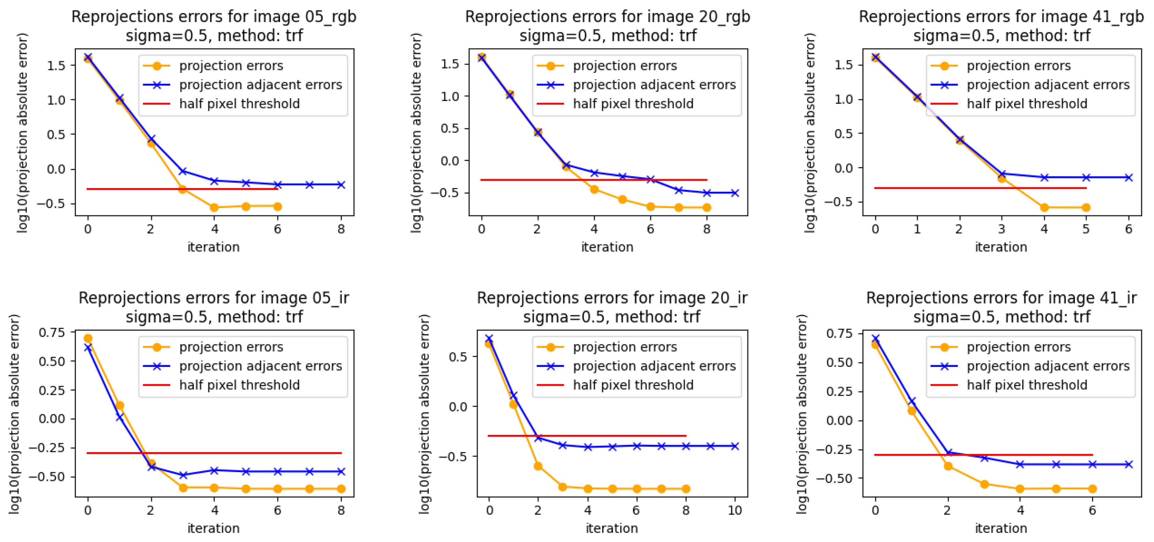
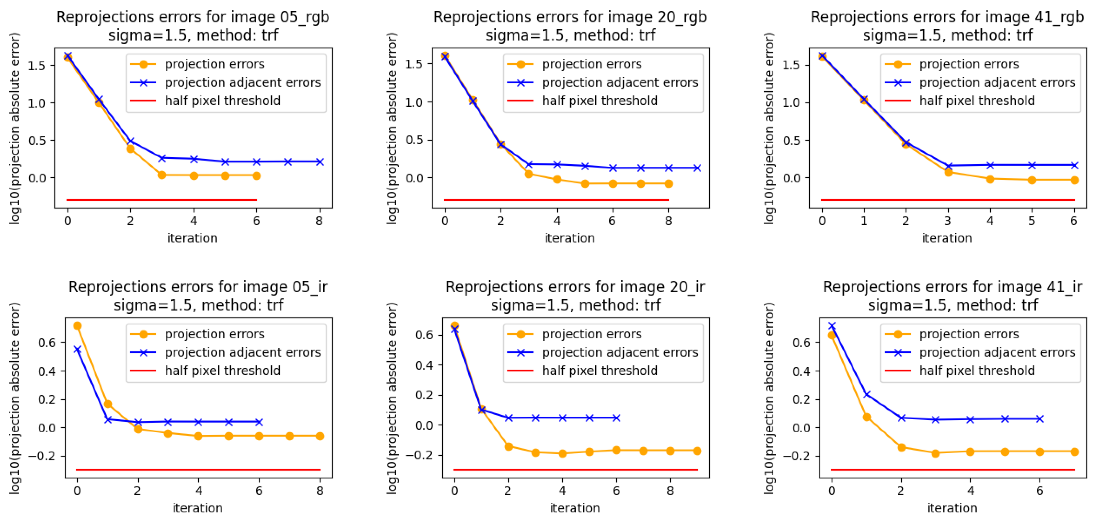
Figure 6 and Figure 7 illustrate typical convergence behavior of the reprojection error for $\sigma =0.5$ px and $\sigma =1.5$ px, respectively. In both cases, a rapid and predominantly monotonic decrease of the error is observed with the half-pixel threshold typically reached within a small number of iterations.

Table 5 and Table 6 report quantitative statistics averaged over 15 randomly selected board poses, with three independent noise realizations per pose. For each noise level, we report the mean, median, RMSE, and maximum reprojection error, the average number of optimizer iterations, the number of iterations required to reach the 0.5 px threshold (when applicable), and the success rate.

A trial is considered successful if the final reprojection RMSE remains below 0.5 px.

High-Resolution RGB Camera

For the RGB camera, the method remains highly stable for localization noise levels up to $\sigma =0.5$ px. The reprojection error increases approximately proportionally to the injected noise, while the success rate remains close to 100%.

For larger perturbations ($\sigma \ge 1.0$ px), a gradual decrease in success rate can be observed. This behavior is expected, as large artificial perturbations distort the geometric consistency between the planar board and its image projection.

Importantly, the mean number of iterations remains nearly constant across noise levels, indicating that convergence speed is only weakly affected by moderate localization noise.

Results in Table 5 and Table 6 were averaged over 15 randomly selected board poses, with three independent noise realizations per pose.

Remark: Each optimizer iteration corresponds to four Cayley evaluations.

For the high-resolution RGB camera, the method remains highly stable for localization noise levels up to $\sigma =0.5$ px. The reprojection error increases approximately proportionally to the injected noise, while the success rate remains close to 100%.

For larger perturbations ($\sigma \ge 1.0$ px), a gradual decrease in success rate can be observed. This behavior is expected, as large artificial perturbations distort the geometric consistency between the planar board and its image projection.

Low-Resolution IR Camera

For the low-resolution IR camera, the effect of localization noise is more pronounced due to lower spatial resolution and inherently higher baseline measurement uncertainty.

Nevertheless, the overall degradation pattern follows the same trend as in the RGB case. For moderate noise levels, convergence remains stable and monotonic, and the iteration count does not exhibit instability or divergence.

The similarity of convergence behavior across heterogeneous sensors confirms that the optimization framework remains stable under realistic measurement noise conditions and that no instability specific to the Cayley parameterization is observed.

Overall, these experiments demonstrate that the observed reprojection error statistics reflect the algorithm’s sensitivity to realistic localization noise. Rather than relying solely on synthetic benchmarks, the inclusion of both high-resolution RGB and low-resolution IR sensors provides an empirical assessment of robustness under diverse practical conditions.

The effective number of state updates required to reach the half-pixel reprojection error threshold is approximately five for ProCay78 in the high-resolution RGB case (Table 5).

Number of Effective Optimizer Steps

The number of effective optimizer steps required to reach the 0.5 px reprojection threshold is approximately five in the high-resolution RGB case (Table 5).

For comparison, Terzakis and Lourakis report in [4] that SQPnP typically requires between 10 and 15 iterations of their constrained optimization stage. While the iteration mechanisms differ and are not directly comparable, this observation indicates that the deterministic canonical initialization employed in ProCay78 leads to rapid attraction toward the low-error region.

These results confirm that the proposed initialization strategy and Cayley-based optimization remain stable under both realistic and artificially amplified localization noise, without exhibiting oscillatory or divergent behavior.

Reproducibility Context

As for the parameters of the optimizer scipy.optimize.least_squares, in our experiments they are always set to their default values, except for the choice of the loss parameter: loss=’soft_l1’ if method==’trf’ else ’linear’. The loss option determines here the smooth approximation of $l_1$ (absolute value) loss. It is a verified choice for robust least squares.

6. Discussion and Conclusions

In this work, we proposed the PnP-ProCay78 algorithm as an alternative approach to estimating the camera pose with respect to a planar calibration object. The starting point is the classical quadratic formulation of the reconstruction error, known from the SQPnP algorithm; however, the key differences concern the selection of initial points and the parameterization of rotations.

Experimental evaluation on heterogeneous datasets acquired from high-resolution RGB cameras and low-resolution thermal cameras demonstrates that the proposed method achieves reprojection accuracy comparable to state-of-the-art OpenCV implementations such as SQPnP and IPPE.

Convergence analysis in Cayley space reveals stable and rapidly contracting optimization trajectories, with consistent behavior across sensors of significantly different resolution and noise characteristics.

The most important theoretical observation is the exploitation of the kernel structure of the reconstruction error matrix $\Omega$ in the planar case. It was shown that the canonical basis vectors $e_3$, $e_6$, and $e_9$ always belong to $ker(\Omega )$, while the minimal positive values of the cost function consistently occur along the directions $e_7$ and $e_8$. Since the value of the quadratic form $x^{⊺}\Omega x$ corresponds to the reconstruction error for $x\in {\mathbb{R}}^9$, it can be computed directly from the definition of the reconstruction error itself. As a result, during the initialization stage, the PnP-ProCay78 algorithm does not require the explicit construction of the matrix $\Omega$.

However, in order to continue the optimization process efficiently, the algorithm requires fast computation of the translation vector using the relation $t=\mathcal{T}r$, where $\mathcal{T}\in {\mathbb{R}}^{3\times 9}$ is a constant, data-dependent matrix. For this reason, the algorithm relies on the stationarity condition of the reconstruction error function ${\mathcal{E}}^2$ with respect to translation. There is no direct dependence on the numerical values of the reconstruction error itself; instead, the dependence is on the minimizing translation

$$t_{min}\doteq arg\underset{t\in {\mathbb{R}}^3}{min}{\mathcal{E}}^2(r,t)=\mathcal{T}r.$$

By using the reprojection error directly as the loss function in the nonlinear optimizer, while indirectly relying on the reconstruction error through the stationarity condition, the PnP-ProCay78 algorithm can be regarded as a hybrid method with respect to these two loss functions.

Unlike SQPnP, which initializes the optimization from saddle points obtained via a full spectral decomposition, the PnP-ProCay78 algorithm relies solely on the relation between the diagonal elements ${\Omega }_{77}$ and ${\Omega }_{88}$. This leads to an unambiguous and fully deterministic selection of two antipodal starting points in Cayley space.

The use of the Cayley parameterization enables a reduction of the state–space dimensionality to three independent variables, allowing standard least-squares solvers such as the Trust Region Reflective method and the Levenberg–Marquardt algorithm to be employed. An analysis of the optimization trajectories in Cayley space provides additional visual insight into the convergence process, both for high-resolution RGB cameras and for very low-resolution thermal cameras. Notably, despite substantial differences in input data quality, the trajectories exhibit strong spatial similarity and close convergence for both modalities.

Comparative experimental results indicate that, in terms of reconstruction error, PnP-ProCay78 achieves accuracy practically identical to SQPnP and slightly superior to IPPE, while maintaining a considerably simpler algorithmic structure. Although the computational time required to initialize the camera pose in complete calibration sequences is negligible compared to other steps in the calibration process, significantly reducing the number of optimization steps to achieve sub-half-pixel accuracy has research value.

The results indicate that a carefully chosen rotation parameterization combined with a transparent optimization framework can yield competitive numerical performance while maintaining geometric interpretability and structural simplicity.

An additional contribution of this work is the demonstration of a coherent pose analysis for RGB and thermal cameras within a multi-sensor system. Although the PnP-ProCay78 algorithm does not explicitly incorporate sensor-specific information, the experiments show that a joint analysis of optimization trajectories can serve as a valuable diagnostic tool in integrated RGB–IR vision systems.

In summary, the proposed PnP-ProCay78 algorithm offers a conceptually simple, geometrically transparent, and attractive alternative to existing PnP solutions for planar scenes. Its reliance on standard geometric models and classical optimization techniques makes it particularly suitable for both research applications and educational use. Potential directions for future work include extending the method to quasi-planar scenes and investigating its properties in the context of joint calibration of multi-camera systems.