Traffic Forecast and Hybrid Optimization-Based Vehicle Route Planning for Cold Chain Logistics

Abstract

The Vehicle Routing Problems with Time Windows (VRPTW) has remained a classic and continuously studied problem since its introduction. With the rapid growth of cold chain product distribution demands, VRP research has become increasingly important for guiding real-world scheduling decisions. However, most studies focus on further subdividing new scenarios and constraints, often overlooking fundamental real-world applications. This includes the impact of unknown road conditions on costs, rough cost modeling, and poor algorithm adaptability to high-dimensional cold chain constraints. To address these three issues, this paper proposes the Spatio-temporal dependency and road network distribution-based traffic forecasting model (STD-RND) to provide region-level traffic scheduling information. The model also constructs cost functions to quantify cargo spoilage, refrigeration, and carbon emissions. Finally, we introduce an Improved Hippo Optimization with Traffic Forecasting (IHTF) that incorporates traffic prediction to enhance the solution quality of the VRPTW in cold chain scenarios. To strengthen optimization performance and prevent premature convergence to local optima, we integrate several enhanced strategies, including chaotic mapping, dynamic Cauchy mutation, and an escape mechanism. Through a series of experiments on the Solomon dataset and simulation datasets based on real road networks, we demonstrate that the proposed algorithm shows consistent superiority and effectiveness.

1. Introduction

In recent years, the demand for cold chain product distribution, represented by flowers and fresh food, has surged, leading to significant growth in the cold chain industry. This expansion has brought the VRP problem in cold chain scenarios to the forefront. The additional costs of refrigeration, the spoilage costs of refrigerated goods, and the high energy consumption and emissions of refrigerated vehicles contribute to severe carbon pollution, creating a significant barrier between research on cold chain VRP and real-world applications [1]. As a result, determining how to efficiently plan delivery routes, while meeting customer demand and minimizing costs and environmental impact, has become a critical issue in the application of cold chain VRP.

At the same time, with the increasing number of vehicles, unpredictable and complex traffic conditions have become a key factor affecting scheduling decisions, and they are the main reason for missing the ideal delivery time window. According to a report from a major Chinese platform in 2023, complaints arising from delivery delays accounted for 37%, with traffic congestion being the cause in 42% of cases. Furthermore, unknown road conditions also lead to cost surges and increased environmental pollution in congested areas. Therefore, incorporating real traffic conditions into scenario modeling is both realistic and feasible.

In previous research on VRP problems that consider real traffic conditions during delivery, many scholars have relied on static map data or simple periodic function models, overlooking the complexity of route planning and dynamic traffic conditions. Instead, they often assume that there is only one Euclidean distance path between each customer point and that traffic conditions along the route remain constant. In reality, we must recognize that all costs are directly or indirectly related to travel time on specific roads.

The current situation highlights the existing weakness in research on VRP problems that deal with real traffic conditions [2]. Studies have shown that, compared with passively responding to congestion after it occurs using reinforcement learning-based route planning, proactively forecasting traffic conditions is undoubtedly the best strategy for addressing congestion. Therefore, developing a cold chain VRP model that integrates real-traffic predictions is of great significance. It not only reduces congestion-related delays during delivery but also helps balance traffic flow across different segments of the road network.

The main contributions of this work are as follows:

(1) This paper designs a time-dependent VRPTW mathematical model for cold-chain distribution that integrates real road-condition prediction. It constructs an application-level model covering travel distance, flower spoilage cost, refrigeration cost, carbon-emission cost, and time-window penalty cost, which further promotes the deep coupling between dynamic traffic conditions and multi-cost objectives in cold-chain logistics. More efficient and realistic routing schemes are obtained by minimizing the mixed-integer linear programming objective.

(2) This paper proposes an Improved Hippopotamus Optimization Algorithm with Traffic Forecasting (IHTF) that incorporates real-world road-condition prediction. The algorithm integrates a Spatio-temporal Dependency and Road Network Distribution-based forecasting model (STD-RND). On the basis of capturing spatio-temporal dependencies via GCN and GRU, a customized Feature Enhancement Matrix is designed to introduce multi-source external features, and an attention mechanism is adopted to extract implicit feature correlations, thereby improving the accuracy of one-day-ahead prediction.

(3) Based on the original Hippopotamus Optimization (HO) framework, this paper develops a hybrid optimization algorithm by constructing a set of diverse hybrid operators and an escape mechanism. These designs strengthen global exploration capability and convergence speed, as well as improve solution quality. Experiments on simulation datasets constructed from real road networks verify the feasibility and stability of the IHTF algorithm, providing a practical solution for time-dependent routing problems in cold-chain logistics scenarios.

2. Literature Review

In current research on cold chain VRP, scholars have begun to expand the focus towards applied-level studies, innovatively incorporating additional cost functions and constraints into the model. Yang et al. [3,4] introduced both temperature control energy consumption and nonlinear spoilage cost functions into the cold chain problem model, solving it using the NSGA-II algorithm combined with a hybrid simulated annealing operator. Zhang et al. [5] proposed a green VRP model that considers carbon trading prices, solving the problem with an improved genetic algorithm featuring elite retention strategies and multiple crossover and mutation mechanisms to enhance global search capability and convergence speed. Riccardo et al. [6] applied the “height profile method” to subdivide each arc into multiple equal-length segments, calculating the impact of actual slopes on energy consumption and emissions. Ma et al. [7] integrated environmental factors such as wind speed, wind direction, temperature, slope, and asphalt type into a model that evaluates their effects on fuel consumption and carbon emissions, creating a micro-level fuel consumption model. Ren  et al. [8] proposed a vehicle routing optimization model that couples carbon emission costs with fuel types, significantly enhancing the economic and environmental efficiency of green logistics path optimization by introducing local search operations into the traditional GA framework. Zhang et al. [9] proposed a pharmaceutical logistics model that incorporates transportation temperature control and a drug potency decay model, making a theoretical contribution to pharmaceutical delivery scenarios. Liu et al. [10], in their study on multi-center fresh agricultural product delivery VRP, introduced a hybrid algorithm combining water wave optimization (WWO) with adaptive ALNS. This approach incorporated multiple local search strategies, effectively avoiding premature convergence and improving solution quality and stability. Jiang et al. [11] built a two-stage cold chain VRP model with dynamic customer demands, using a genetic algorithm with multiple destruction and repair operators. Iksan et al. [12] focused on path planning for maritime passenger vessels, proposing a hybrid genetic algorithm with a fixed radius nearest neighbor (FRNN) heuristic to minimize passenger transfer times. Lastly, Frías et al. [13] presented a hybrid algorithm for green logistics, integrating clustering with ant colony optimization, and introduced two strategies-Free Ant and Restricted Ant-to minimize energy consumption.

Carbon emissions from the transportation industry account for over 10% of global total emissions, with transportation activities as the primary source. Road traffic conditions serve as a key factor affecting the punctuality and costs of transportation operations. Therefore, it is imperative to incorporate real-world traffic issues in the distribution process into scenario modeling. In the field of time-dependent VRP, most studies that target real-traffic traffic still rely on static road networks or fuzzy mechanisms to approximate road conditions. These approaches overlook how complex traffic patterns and rapidly changing traffic flows shape the development and practical performance of VRP models. Vrani et al. [14], working with a real pharmaceutical distribution scenario, designed three time-dependent travel-time matrices (optimistic, most likely, pessimistic). Their uncertainty-aware modeling adds realism and captures greater operational complexity. Akkerman et al. [15] used reinforcement learning for route planning and trained a Markov model on average congestion patterns to reduce road uncertainty while supporting dynamic customer arrivals and real-time dispatching. Heidari et al. [16] developed a dynamic re-routing system for cold-chain VRP that responds to demand fluctuations and congestion, combining MILP with dynamic clustering. Sze et al. [17] built a dynamic re-routing framework capable of rapidly adjusting routes during unexpected events. Pooja et al. [18] further summarized the evolution of VRP research from static toward dynamic and real-traffic paradigms. Despite these efforts, current work still lacks robust solutions for modeling real, highly complex city-level traffic. Nyako et al. [19] addressed traffic by dividing the day into static time slices, assigning each road segment an average speed and fuel-consumption profile, and then using machine-learning-enhanced NSGA-II for optimization. Patil et al. [18] introduced reinforcement learning to autonomously choose routes and reduce congestion and travel time, but the system reacts only to the current state. Elgharably incorporated uncertainty into green VRP by modeling travel and service times as normally distributed variables, but the representation of travel time remains overly vague. Ma et al. [7] proposed a vehicle-routing model that integrates time-dependent characteristics and environmental pollution factors. Their framework systematically accounts for wind speed, temperature, slope, and asphalt type when estimating fuel consumption and uses fuel use as a proxy for optimizing carbon emissions. They designed a hybrid GWO-MLP algorithm that couples neural-network predictions with grey wolf optimization. Xidias et al. [20] combined fuzzy logic with the A* algorithm and an improved genetic algorithm. They mapped actual distance and traffic conditions to virtual distance via a Mamdani fuzzy inference system, quantified the impact of traffic uncertainty on routing planning, and achieved integrated optimization of Vehicle Routing Problem (VRP) and Motion Planning Problem (MPP). However, their fuzzy mechanism still fails to fully capture the dynamic characteristics of real-time traffic flow. Nisyrios et al. [21] pointed out in a systematic review that although existing studies on CAV traffic and fleet management have considered optimization in mixed traffic environments, most work remains limited to single-lane or isolated intersection scenarios and lacks adaptation to multi-lane and multi-intersection complex traffic flows. Furthermore, the deep integration between traffic prediction and VRP still represents a critical research gap. Xue et al. [22] used an adaptive fractional Kalman filter to predict traffic speed and then designed an adaptive cuckoo search algorithm based on those predictions.

However, very few studies generate accurate forecasts beforehand, and many systems can only react after congestion appears—leading to costly last-minute route adjustments. Although recent work has begun to incorporate time-dependent elements into VRP, most models still treat time-varying speeds as simple functions or fuzzy approximations, which cannot capture the real complexity of logistics traffic. Furthermore, research that tightly integrates traffic prediction with the VRP optimization process remains scarce and requires deeper investigation.

Scholars in the relevant research field have conducted in-depth studies on the Vehicle Routing Problem (VRP) from multiple aspects, including constraints, research objects, and solution strategies, but several challenges remain. Real-time road condition models are still overly rough, cost accounting often lacks scientific rigor, and many algorithms struggle when facing high-dimensional and complex VRP models. To address these issues, this paper constructs a cold-chain VRP model that integrates road condition prediction, combining two core issues: vehicle routing planning (VRP) and traffic forecasting. Given the complex combinatorial optimization nature of cold chain transportation scenarios with road condition prediction, the STD-RND forecasting model proposed in this paper integrates GCN and GRU to extract the irregular network topology of real road traffic networks and a more lightweight temporal dependency feature extractor. Furthermore, the feature enhancement matrix and attention mechanism designed in this paper extract implicit dependencies between multi-source external features (POI, day of the week, and weather) and traffic speed, which can significantly improve prediction accuracy.

Regarding the large solution space scale and complex solving characteristics of this scenario, we leverage the excellent exploitation efficiency and solving capability of the basic HO algorithm framework. We specifically propose a Cauchy mutation optimization operator, an adaptive local search operator, and an adaptive escape mechanism based on the Metropolis criterion to enhance the algorithm’s optimization capability and convergence speed in cold-chain VRP scenarios with road condition prediction.

3. Problem Analysis and Mathematical Model

This study focuses on the Vehicle Routing Problem with Time Windows (VRPTW) in a time-dependent cold-chain distribution setting. We build an intelligent transportation system (ITS) for cold-chain logistics, consisting of delivery vehicles, a central depot, and customer nodes distributed across a real road network. With accurate traffic forecasts, the ITS plans routes in advance and assigns delivery tasks to vehicles, specifying both customer sequences and travel paths. Guided by the scheduling system, each vehicle avoids congested roads and serves customer nodes in order.

3.1. Real-Traffic Prediction Model

This model focuses on accurate day-ahead traffic predictions, such as congestion and vehicle speed, to assist the dispatch center in making cost-minimizing route planning.

3.1.1. Road Travel Time

Road traffic speed serves as a key variable that drives subsequent decisions and cost evaluation. Before the system plans delivery routes, it is difficult to observe and forecast each vehicle’s continuous speed over time. However, since vehicle speed remains relatively stable over short intervals, we use a predicted discrete-time function to calculate the travel time between customer nodes. We will apply the same idea later to evaluate each component of the cost model. Specifically, we decompose the road segment between customers i and j into a set of predicted road links, ${\mathit{d}}_{\mathit{ij}}=\{d_1,d_2,d_3\dots ,d_l\}$, which represents the real road-link set between the two customers on the actual map. We usually split the path at road intersections, so each link corresponds to a road section between two adjacent junctions. For each link $d_i$, the predicted speed under the adopted time granularity is denoted as $V_i\left(t_s\right)$, where $t_s$ is the time when the vehicle enters the link. The resulting travel time from customer i to customer j is then given by

$$t_{ij}=\sum _{i,s=1}^l{\displaystyle \frac{d_i}{Vi\left(t_s\right)}}.$$

(1)

3.1.2. Spatiotemporal Dependency and Attention Based Prediction Model

Since traffic conditions always exhibit periodic and stage-wise changes over time, this paper uses GRU to learn the short-term patterns of temporal dependencies between nodes. The GRU model avoids the vanishing and exploding gradient issues that often affect traditional RNN models. Compared with LSTM, it also features a simpler structure, fewer parameters, and faster training speed. For the spatial dependencies among road nodes, we choose GCN to depict the complex topology of urban road networks, overcoming the limitation that RNNs only apply to regular structures. Most importantly, we recognize that road condition prediction depends not only on historical traffic flow data but also on latent and complex relationships imperceptible to humans, such as whether it is a holiday and weather conditions.

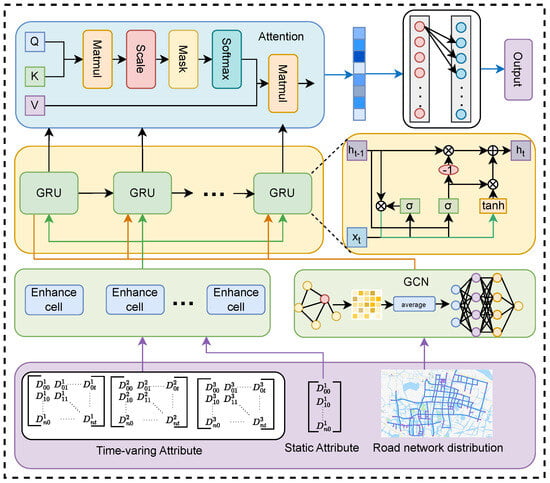
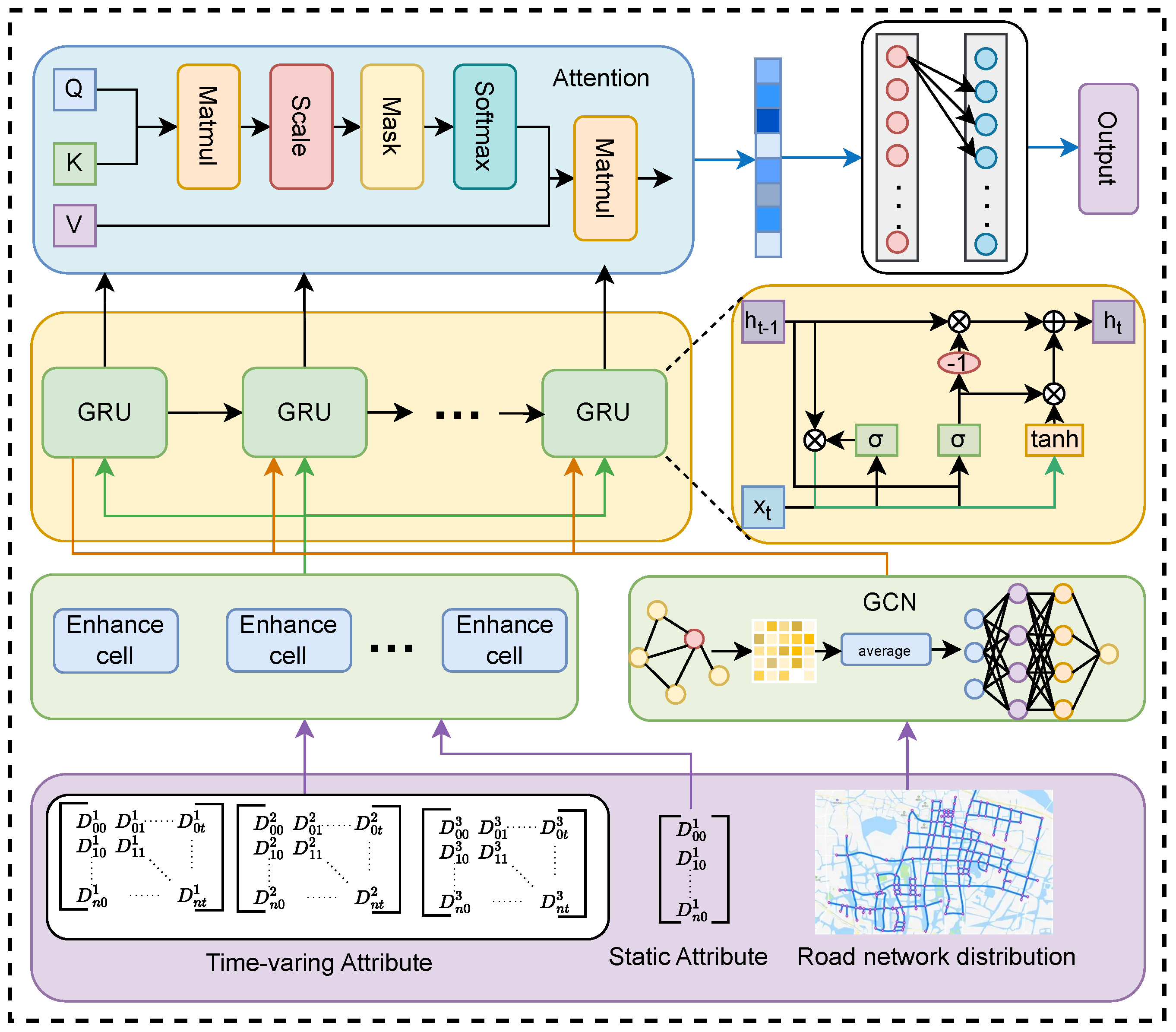
Therefore, we construct a feature enhancement matrix and integrate it into the prediction model, using a multi-head attention mechanism to extract the relationships unrecognizable to the human brain. The structure of the STD-RND model proposed in this paper is shown in Figure 1.

From bottom to top, we design a feature enhancement matrix $K=\{S,T,X_t\}$ to introduce the Static Attributes of road nodes (such as POIs along the roads) and Time-varying Attributes, greatly strengthening the latent connections among road nodes. The static attribute $S\in R^{n\times p}$ represents static social attributes that do not change over time but still affect traffic states, such as whether an area is a park, business district, hospital, or school zone. Here, n denotes the number of prediction nodes, and p denotes the number of fixed information categories. The time-varying attribute $T\in R^{n\times t\times j}$ refers to time-varying features that change over time and directly affect traffic. For example, weekday indicators directly determine the real-time traffic volume of road segments, while the weather-change matrix directly influences drivers’ driving behaviors. We fuse these multi-source features with potential correlations to form an enhancement matrix, where j denotes the number of time-varying information categories.

It then feeds the expanded feature matrices into the spatio-temporal dependency model. Within this model, the GCN extracts spatial dependencies among nodes in the road topology. Multiple graph convolution layers capture feature interactions between each node and its higher-order neighborhoods. We then pass the resulting spatial feature matrix, together with the augmented feature matrix, into the GRU gating structure. The reset and update gates decide which temporal effects to retain or discard, allowing the network to capture sequential correlations among nodes and learn dynamic time series variations. Next, an attention mechanism captures global temporal dynamics and spatial correlations in traffic flow. It computes a context vector that represents the overall trend of traffic-state evolution, and uses it to support future traffic prediction. Finally, a fully connected layer produces the prediction output.

3.2. Problem Description and Assumptions

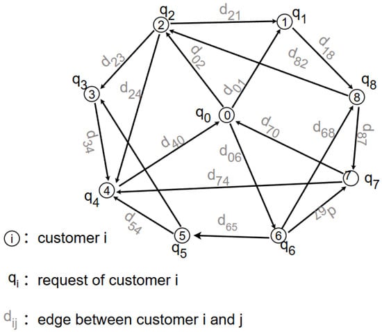
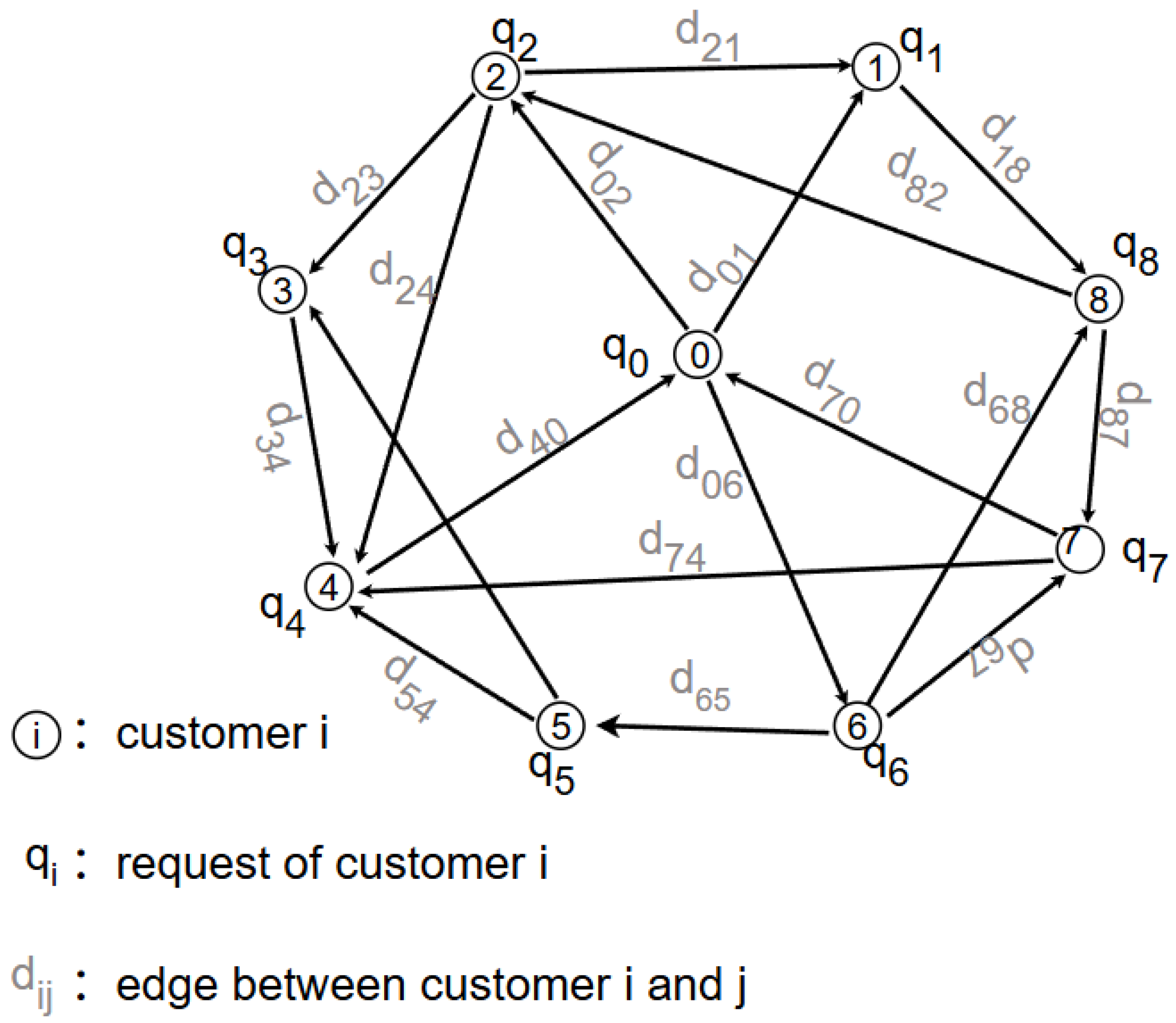
This paper formulates a mathematical VRPTW model for cold-chain distribution.The model is defined on a directedgraph $G=(N,E)$, where $N=\{i\mid i=0,1,2,\dots ,n\}$ denote the set of nodes, including the depot (i = 0) and n customer nodes. Let $E=\{d_{ij}\mid i,j=0,1,2,\dots ,n\}$ denote the edge set, where each $d_{ij}$ represents a feasible connection between nodes i and j. An example is shown in Figure 2, the network contains one depot, 8 delivery nodes, and 17 connected road segments. Each vehicle has a maximum capacity limit. Customer i requests a demand $q_i$, and every demand does not exceed the vehicle capacity. Vehicles must serve each customer within its specified service time window. The parameters and variables involved in the model are defined as shown in

Table 1. Parameters and variable symbol description table.

Symbol	Meanings
$q_i$	Demand for flowers at customer point i, (t).
$s_i$	Service time at customer point i, (h).
Q	Maximum loading capacity of a delivery vehicle, (t).
$q_{ij}^k$	Actual load of vehicle k traveling from customer i to customer j, (t).
$d_{i}j$	Distance from point i to j (i = 0: distribution center), (km).
$t_i$	Arrival time of the vehicle at point i, (h)
$Q_0$	Initial quality of the product, (t)
$\epsilon$	Carbon emission factor of the fuel, (kg/L)
w	${\mathrm{CO}}_2$ emission coefficient for refrigeration, (kg/L)
m	Unloading efficiency, (t/h).
$\delta$	Coefficient of Case Deterioration, Unitless, represents the scaling factor for magnification or reduction.
F	The rate of heat exchange between the vehicle compartment and the outside environment, w/(m${}^2$ · K).
$\mathrm{\Delta }T$	The temperature difference between the interior of the carriage and the outside, (K).
$E_a$	Activation energy required for spoilage of fresh goods, (J/mol).
R	Arrhenius gas constant, (j/mol · K).
$P_{\varphi }$	Unit cost penalty coefficient for early arrival per unit time, Proportional coefficient, dimensionless.
$P_{\eta }$	Unit cost penalty coefficient for late arrival per unit time, Proportional coefficient, dimensionless.
$x_{ik}$	Binary variable indicating whether customer i is served by vehicle k, dimensionless.
$x_{ij}^k$	Binary variable indicating whether vehicle k travels from customer i to customer j, dimensionless.

.

The objective is to satisfy all customer service requirements while minimizing total cost, including spoilage cost, travel distance cost, refrigeration cost, carbon emission cost, and time-window penalty cost, thereby maximizing overall profit. The model uses the following notations and assumptions:

(1) During travel, vehicles generate carbon-emission costs and refrigeration costs, and the flowers continuously deteriorate. During service, the engine stays off, so the vehicle does not incur carbon-emission costs; however, opening the doors accelerates flower spoilage.

(2) The vehicle service time operates within a soft–hard mixed time window. Vehicles may arrive earlier or later at the customer’s location, but both scenarios incur a linear penalty cost. Additionally, the vehicle arrival time must not exceed or be earlier than the fixed business hours.

(3) Flower deterioration occurs throughout the entire delivery process, and the spoilage cost increases exponentially with the deterioration rate.

(4) The system distributes only one type of product. All deliveries share similar conditions, including transportation mode, refrigerated-compartment temperature, and product size.

3.3. Mathematical Model for Cold Chain VRP Integrating Traffic Prediction

3.3.1. Spoilage Cost

When a refrigerated vehicle travels, it uses fuel-generated electricity to power the cooling system and keep the compartment at a suitable low temperature, which slows down deterioration. An exponential spoilage rate can describe the decay process of fresh products more accurately. We compute the flower deterioration rate using the Arrhenius equation as

$$K=Aexp\left(-{\displaystyle \frac{E_a}{RT}}\right).$$

(2)

This equation links the reaction rate to temperature. Here, K denotes the reaction-rate constant, which corresponds to the deterioration rate in our setting. A is the Arrhenius constant. $E_a$ is the activation energy. T is temperature. and R is the gas constant. Based on the above formula and food science research, this paper proposes the quality-loss function lqm [23] as

$$lqm={\displaystyle \frac{\mathrm{\Delta }Q}{Q_0}}=\left\{1-exp\left[-Atexp\left(-{\displaystyle \frac{E_a}{RT}}\right)\right]\right\}.$$

(3)

Here, $Q_0$ denotes the initial quality of the fresh product, and $\mathrm{\Delta }Q$ denotes the quality change. t represents the stage time, which in subsequent formulas specifically refers to the delivery time for each customer and the service time. After letting $\theta =Aexp\left(-{\displaystyle \frac{E_a}{RT}}\right)$ represent the deterioration constant and simplifying fixed constants, we obtain

$$lqm=\left[\begin{array}{c}1-e^{-\theta t}\end{array}\right]100\%.$$

(4)

During service, opening the vehicle door keeps the refrigeration unit running, but the large indoor-outdoor temperature gap raises the compartment temperature. We therefore denote the deterioration constant as ${\theta }_1$ and ${\theta }_2$, which represent the spoilage constants when the door is open and closed, respectively. Based on the above, we compute the spoilage cost of refrigerated cargo during distribution as

$$\begin{array}{c}\hfill C_{\mathrm{Spoi}}=\sum _{k=1}^m\sum _{i,j=0}^n{c}_1\left[q_{ij}^k\left(1-e^{-{\theta }_1{t}_{ij}}\right)+\left(q_{ij}^k-q_i\right)\left(1-e^{-{\theta }_2{\displaystyle \frac{q_i}{m}}}\right)\right].\end{array}$$

(5)

In this expression, $c_1$ is a cost-weight factor obtained from our investigation, representing the unit spoilage cost coefficient. $q_i$ is the demand at customer i. m is the unloading efficiency (unloading quantity per unit time). $q_k^{ij}$ is the cargo load carried by vehicle k while traveling from i to j. The travel time $t_{ij}$ comes from segmenting the real route between customers i and j and then aggregating over the predicted speed functions.

3.3.2. Travel Distance Cost

The travel distance, serving as the most intuitive evaluation criterion for a scheduling plan from the perspective of enterprises, is the sum of the distances between each pair of customers sequentially served by each delivery vehicle according to the planned delivery scheme.

$$C_{mile}=c_2\sum _{k=1}^n\sum _{j=0}^n{x}_{ij}^k{d}_{ij},$$

(6)

where $c_2$ denotes the cost weight factor per unit distance, reflecting the significance of mileage in the hybrid optimization objective. $d_{ij}$ represents the delivery distance from customer i to customer j.

3.3.3. Refrigeration Cost

The refrigeration cost consists of two parts: cooling when the door remains closed and additional cooling when the door is open. Building on recent advances in thermal engineering and power systems, we model refrigeration cost through temperature differences, cargo volume, and transport duration. The cooling cost when the door stays closed is

$$\begin{array}{cc}\hfill C_{\mathrm{lock}}=c_3& \sum _{k=1}^l\sum _{i,j=0}^n{x}_{ij}^k(1+\delta )F\left(\sqrt{S_1-S_2}\right)\mathrm{\Delta }T{t}_{ij}.\hfill \end{array}$$

(7)

Here, $c_3$ denotes the cost weight factor for refrigeration. $d_{ij}$ represents the travel distance from node i to node j. The deterioration coefficient $\delta$ reflects extra energy consumption caused by outside temperature and other environmental factors during transport. F describes the vehicle’s thermal conductivity and characterizes the heat-exchange rate between the compartment and the $S_1-S_2$ measure the difference between the outer and inner surface areas of the refrigeration compartment, which reflects the vehicle’s insulation performance. $\mathrm{\Delta }T$ denotes the temperature difference between the compartment interior and the outside environment. Following the same principle, the cooling cost when the door is open is

$$C_{\mathrm{open}}=c_3\sum _{k=1}^l\sum _{i=0}^n\beta \left(0.54{\nu }_k+3.22\right)\mathrm{\Delta }T{\displaystyle \frac{x_{ik}{q}_i}{m}}.$$

(8)

Here, $\beta$ represents the door opening frequency factor, which reflects the rate at which cold air escapes during unloading. $V_k$ denotes the refrigerated compartment volume of vehicle k. We introduce a binary variable $X_{ik}$ to indicate whether vehicle k serves customer i, and $q_i$ represents demand of customer i. For simplicity, we treat the unloading efficiency m as a constant, meaning the quantity unloaded per unit time remains fixed. Combining both parts, the total refrigeration cost becomes

$$\begin{array}{cc}\hfill C_{\mathrm{refri}}& =C_{\mathrm{open}}+C_{\mathrm{lock}}\hfill \\ \hfill & =c_3\sum _{k=1}^l\sum _{i,j=0}^n\beta (0.54{\nu }_k+3.22)\mathrm{\Delta }T{\displaystyle \frac{x_{ik}{q}_i}{m}}+x_{ij}^k(1+\delta )F\left(\sqrt{S_1-S_2}\right)\mathrm{\Delta }T{t}_{ij}.\hfill \end{array}$$

(9)

3.3.4. Carbon Emission Cost

Carbon emission cost comes from fuel combustion due to both vehicle motion (driving/braking) and refrigeration. When vehicle travels, the engine burns fuel and generates carbon emissions. Based on extensive empirical data, prior studies show that a transport vehicle’s fuel consumption increases linearly with its payload [24]. Thus, the fuel consumption rate per unit distance can be written as

$$\xi =\epsilon \left(\mu +q\right)+b.$$

(10)

where $\epsilon$ denotes the carbon emission factor of the fuel. $\mu$ is the vehicle’s empty weight. q is the payload. and b is a constant term, for which we adopt the standard international value. Let $x_{ij}^k$ be a binary variable indicating whether vehicle k travels from customer i to customer j. The carbon emission produced by driving from i to j is

$$C_{drive}=c_4\sum _{k=1}^l\sum _{i,j=0}^n{x}_{ij}^k\left[\epsilon \left(\mu +q_{ij}^k\right)+b\right]d_{ij}.$$

(11)

We typically set the emission factor to 2.62 kg/L [25]. Refrigeration also consumes additional fuel to generate electricity for cooling, which explains why refrigerated vehicles show higher energy use and pollution than conventional trucks. During door-closed transport, refrigeration-related emissions grow with a constant coefficient. During unloading with the door open, we assume the cargo decreases at a constant rate, so the carbon emissions cost from refrigeration decreases linearly. Building on Equation (9), we revise the formulation and obtain the extra refrigeration-induced emissions. Combining these components, we update the total carbon emission cost as

$$\begin{array}{cc}\hfill C_{\mathrm{Carb}}=& c_4\sum _{k=1}^l\sum _{i,j=0}^n\{\beta w(0.54v_k+3.22)\mathrm{\Delta }T{\displaystyle \frac{x_{ik}{q}_i}{m}}+x_{ij}^{k}w(1+\delta )F\left(\sqrt{S_1-S_2}\right)\mathrm{\Delta }T{t}_{ij}\hfill \\ \hfill & +x_{ij}^k[\epsilon (\mu +q_{ij}^k)+b]d_{ij}\}.\hfill \end{array}$$

(12)

where, $c_4$ represents the weight of carbon emission costs, and w stands for the $C{O}_2$ emission factor when the refrigerated truck is cooling.

3.3.5. Time Penalty Cost

Cold chain transportation imposes stricter requirements on delivery timeliness. Customers expect their orders to be serviced within a designated time window. However, because unexpected factors often affect real operations, we adopt a soft–hard mixed time-window penalty scheme. When a delivery falls outside a customer’s service window, the refrigerated vehicle incurs penalties, including: (1) an early-arrival penalty when the vehicle reaches the customer before the earliest allowable time, and (2) a late-arrival penalty when the vehicle reaches the customer after the latest allowable time.

We also force the vehicle’s arrival time to remain within the customer’s business hours; violating this constraint results in an infinite penalty. Based on these rules, the total time-window penalty cost becomes

$$\begin{array}{cc}\hfill C_P=c_5& \sum _{k\in K}\sum _{i\in n}[P_{\phi }max\left(0,{\mathrm{T}}_{early}^i-{\mathrm{t}}_i\right)+P_{\eta }max\left(0,{\mathrm{t}}_i-{\mathrm{T}}_{late}^i\right)].\hfill \end{array}$$

(13)

Here,$c_5$ denotes the unit time-penalty coefficient. $T_{early}^i$ and $T_{late}^i$ represent the earliest and latest allowable service times for customer i. $t_i$ is the actual arrival time of refrigerated vehicle k at customer i. The penalty coefficients $P_{\varphi }$ and $P_{\eta }$ define the unit time penalty for early and late arrivals, respectively.

The objective function is a mixed-integer linear programming objective that minimizes the costs of flower spoilage, refrigeration, carbon emissions, travel distance, and time penalties.

$$minC=C_{Spoi}+C_{mile}+C_{Carb}+C_{refri}+C_P$$

(14)

Subject to:

$$\begin{array}{ccc}\sum _{\mathrm{i}\in \mathrm{N}}\sum _{\mathrm{k}\in \mathrm{K}}{x}_{ik}{q}_i\le Q\hfill & \hfill & \hfill \end{array}$$

(15)

$$\begin{array}{cccc}\hfill & \sum _{\mathrm{k}\in \mathrm{K}}{x}_{ik}=1,\forall \mathrm{i}\in N\hfill & \hfill & \hfill \end{array}$$

(16)

$$\begin{array}{cccc}\hfill & \sum _{\mathrm{i}\in \mathrm{n}}{x}_{ij}^k=x_{ik},\forall \mathrm{i},\mathrm{j}\in N\hfill & \hfill & \hfill \end{array}$$

(17)

$$\begin{array}{cccc}\hfill & \sum _{\mathrm{k}\in \mathrm{K}}{x}_{ij}^k\le 1,\forall \mathrm{i},\mathrm{j}\in N\hfill & \hfill & \hfill \end{array}$$

(18)

$$\begin{array}{cccc}\hfill & \sum _{\mathrm{k}\in \mathrm{K}}\sum _{i\in \mathrm{N}}{x}_{i0}^k=\sum _{k\in \mathrm{K}}\sum _{j\in \mathrm{N}}{x}_{0j}^k\le 1,\forall \mathrm{k}\in K\hfill & \hfill & \hfill \end{array}$$

(19)

$$\begin{array}{cccc}\hfill & x_{ik}(x_{ik}-1)=0,\forall \mathrm{i}\in N,\forall \mathrm{k}\in K\hfill & \hfill & \hfill \end{array}$$

(20)

$$\begin{array}{cccc}\hfill & x_{ij}^k(x_{ij}^k-1)=0,\forall i,j\in N,\forall \mathrm{k}\in K\hfill & \hfill & \hfill \end{array}$$

(21)

$$\begin{array}{cccc}\hfill & x_{ij}^k+x_{ji}^k\le 1,\forall i,j\in N\mathrm{and}i\ne j,\forall k\in K\hfill & \hfill & \hfill \end{array}$$

(22)

$$\begin{array}{cccc}\hfill & \sum _{\mathrm{i}\in \mathrm{N}}\sum _{\mathrm{k}\in \mathrm{K}}{x}_{0i}^k\le K,\forall \mathrm{i}\in N,\forall \mathrm{k}\in K\hfill & \hfill & \hfill \end{array}$$

(23)

In the proposed model, the objective function (14) represents the optimization goal of minimizing the various mixed-integer linear programming objectives described above. Equation (15) stipulates that the total cargo carried by each delivery vehicle during the distribution process must not exceed its maximum weight capacity. Equations (16)–(18) constrain each demand point to receive service from only one vehicle per trip, thus avoiding redundant deliveries. Equation (19) ensures that all vehicles depart from the distribution center and return there after completing their deliveries. Equations (20) and (21) introduce binary variables, adding logical constraints to the model. Equation (22) specifies that vehicles can only travel in one direction during the delivery process. Finally, Equation (23) limits the total number of delivery vehicles to the maximum number available at the distribution center.

4. The Proposed IHTF Algorithm

4.1. Description of IHTF

Although the VRPTW model proposed in this paper introduces extra variables and constraints, it remains a derivative of the classical VRPTW model and preserves similar computational principles and complexity. To handle the increased difficulty of this expanded formulation, we enhance the Hippopotamus Optimization algorithm (HO). HO, introduced by Ohammad et al. [26] in 2024, is a swarm intelligence algorithm inspired by the social behavior of hippopotamuses. It offers strong global search ability and effective local exploitation capability while maintaining a good balance between exploration and exploitation qualities that are especially valuable when dealing with high-dimensional VRP search spaces.

HO mainly designs a three-stage solution movement mode by simulating the social behaviors of hippo groups in nature, abstracting the position updating, defending, and escaping of hippo groups into local movement and global exploration strategies for individual solutions. Meanwhile, targeting the ever-changing traffic conditions in the unique cold-chain VRP scenario, as well as the typically large-scale customer groups in cold-chain logistics scenarios, we design a hybrid hippopotamus optimization algorithm (IHTF) that incorporates real-time road condition prediction. Furthermore, thanks to the predicted input obtained from the introduced STD-RND model based on GRU and GCN, the algorithm acquires anticipatory traffic prior knowledge for the ITS, thereby significantly enhancing the practicality of scheduling decisions. Therefore, this paper adopts a hybrid optimization algorithm based on the HO basic framework, combined with an excellent road condition prediction module, to solve the time-dependent cold-chain Vehicle Routing Problem with Time Windows (VRPTW).

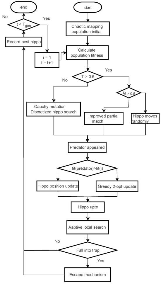
The algorithm flow chart is shown in Figure 3. Based on the basic framework, we introduce genetic operators to enhance the IHTF algorithm’s ability to explore large solution spaces and shorten convergence time, and integrate VNS to improve solution quality. We also incorporate a Cauchy mutation operator with adaptive probability to enhance population diversity and prevent the algorithm from falling into local optima prematurely. Most importantly, we newly construct an Escape Mechanism. All the above solutions are cleverly coupled together, greatly improving the solving capability of the hybrid algorithm in the research scenario of this paper.

Like other swarm-intelligence algorithms, our improved method includes three essential stages: model and population initialization, fitness evaluation, and iterative solution updating until the optimal result is obtained. At the start of each run, we initialize all parameters and generate the initial population using chaotic mapping. The algorithm then performs a broad global search followed by focused local refinement to update the positions of all hippos. Next, we compute the fitness of the initial population and identify the leader hippo, which represents the current best solution. The algorithm then updates all individuals and investigates the surrounding search region.

After that, we simulate predator encounters to force the population to flee from local optima, expanding exploration. VNS further simulates collective escape behavior, helping the population locate safer and better positions nearby and strengthening local exploitation.

In the next step, the Trap Escape Mechanism prevents the population from circling within a narrow region. Inspired by the Metropolis criterion, this mechanism evaluates long-term potential rather than short-term advantage, allowing the algorithm to pursue promising regions even when they are not immediately optimal. The improved algorithm balances IHTF’s strong exploration and exploitation abilities and maintains excellent refinement capability. Through adaptive probabilities, it uncovers hidden structural information during iteration and searches deeper within the latent solution space. When applied to vehicle routing optimization, the algorithm identifies the optimal delivery routes and corresponding costs. The specific algorithm solving process is shown in Algorithm 1.

Algorithm 1 Improved Discrete Hippopotamus Optimization Algorithm (IHTF).

Input:  Hippo population size ($pop\_size$), Maximum number of iterations ($Ma{x}_{i}terations$), Jump coefficient (m). Output:  The best population of hippos.   1: Initialize parameters, Chaotic mapping generate initial population, Calculate fitness obtain the leader hippo;   2: for iter $t=1,2\dots ,Max\_iterations$ do   3:        for $Hippo$$i=1,2\dots ,T$ do   4:              if $i<pop\_size/2$ then   5:                    if $T>0.6$ then   6:                         Cauchy mutation   7:                         Improved hippo move   8:                    else   9:                         if $r_6>0.5$ then 10:                               Improved partial match 11:                         else 12:                               Hippo moves randomly 13:                         end if 14:                    end if 15:              else 16:                   Predator appeared 17:                   if Predator fitness > Hippo${}_i$ then 18:                         Hippo position update 19:                    else 20:                         Greedy 2-opt update 21:                    end if 22:              end if 23:        end for 24:        for $Hippo$$i=1,2\dots ,T$ do 25:              Adaptive local search 26:              if $Hipp{o}_i$ Fall into trap then 27:                    while $n>5$ do 28:                         Reverse mutation 29:                         if Meet metropolis criteria then 30:                               Accept new solution 31:                         end if 32:                    end while 33:              end if 34:        end for 35: end for

4.2. Encoding-Decoding Strategy

The encoding process is a crucial step in algorithm design. IHTF employs a natural number encoding method. The length of the chromosome corresponds to the total number of customers to be served, with each chromosome representing an initial solution. During the decoding of chromosomes, the solution is segmented into delivery routes based on constraints such as vehicle capacity and time windows. The number 0 is added at the start and end of each sub-route to indicate that the route begins and ends at the distribution center. For example, 0-5-4-6-0-1-9-7-10-0-2-8-3-0 represents three vehicle routes: Vehicle 1’s route is 0-5-4-6-0, Vehicle 2’s route is 0-1-9-7-10-0, and Vehicle 3’s route is 0-2-8-3-0 (where “0” denotes the distribution center).

To obtain a more excellent initial population in high-dimensional space and enhance the potential prospects of individuals throughout the high-dimensional solution space, our proposed IHTF algorithm utilizes chaotic mapping. This approach allows the population to be more randomly and uniformly distributed across the high-dimensional solution space. During subsequent iterative solving processes, the population moves towards the potential theoretical optimal individuals from different angles, enabling the broadest exploration of potential evolutionary directions. This results in more promising population seed individuals, increased population diversity, and enhanced algorithm performance and solution quality

4.3. Cauchy Mutation Based Hippo Movement

In the first stage (adolescent exploration), the hippos move freely and randomly within the herd to explore the local search space. The multi-directional random-movement strategy also strengthens global exploration. When the adaptive iteration factor $T=exp\left(-{\displaystyle \frac{t}{T}}\right)>0.6$, immature hippos update their positions within the river or pond region, reflecting the algorithm’s exploration of the current local area. HO performs well on many continuous-optimization problems, demonstrating its strong algorithmic capability. However, for discrete problems like VRP, we designed a discretized hippo optimization operator combined with Cauchy mutation, and the movement strategy of immature hippos is as

$$x_i^{\mathcal{FB}}=x_i+Cauchy(m,\gamma )\left(D_{\mathrm{hippo}}-\mathcal{M}{G}_i\right).$$

(24)

Let $x_i^{\mathcal{FB}}$ denote the i-th immature hippo in the population, and let $D_{\mathrm{hippo}}$ denote the leader hippo identified by the objective function. We select $\mathcal{M}{G}_i$ as a random hippo from among those whose fitness lies around the population mean. Fitness corresponds to the derivative of the optimization objective. Most immature hippos stay close to their mothers, but they sometimes wander due to curiosity. To simulate this behavior, we apply the long-tailed characteristics of Cauchy mutation to adjust positions randomly. The adaptive Cauchy-mutation probability is defined as

$$Cauchy(x,m,\gamma )={\displaystyle \frac{1}{\pi }}\left[{\displaystyle \frac{\gamma }{{\left(x-m\right)}^2+{\gamma }^2}}\right].$$

(25)

Here, m is the jump variable whose optimal value we determine experimentally. Our convergence tests show that $m=0.2$ gives the fastest convergence and highest solution quality. Variable x is a random value in $[0,1]$ generated at each mutation step. Parameter r is the scale parameter that controls the width or dispersion of the distribution. We also introduce an iteration-dependent adaptive factor $\gamma =exp({\displaystyle \frac{t}{T}}-1)$ that adjusts parameters dynamically, balancing exploration and exploitation during the search.

By combining these enhancements, the algorithm expands its search range in the early stages to sample as many feasible regions as possible and avoid premature convergence. In later stages, a smaller inertia weight refines the search and extracts higher-quality solutions, strengthening the algorithm’s local-search capability and improving its ability to lock onto the true global optimum.

4.4. Partially Matched Crossover

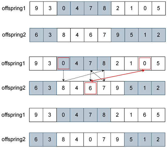
To simulate the curiosity-driven behavior of immature hippos venturing away from their mothers to explore the surrounding solution space, we employ the partially matched crossover (PMX) operator to exchange segments of gene sequences between two parent individuals. Extensive research has demonstrated the superior exploration capability of the PMX operator, along with its ability to accelerate algorithm convergence. This crossover operator stochastically swaps gene segments between parents to produce two offspring that inherit characteristics from both individuals, thereby enhancing their adaptability to the problem.

In the proposed hybrid hippo algorithm, the current immature hippo individual is crossed with the leading hippo (the optimal solution) as parents. This approach not only facilitates the inheritance of superior gene segments but also promotes faster convergence. Given the real-value encoding adopted in this study, a two-point crossover mechanism is utilized for gene exchange between individuals. Specifically, two request points are randomly selected along the routes, and the gene sequences between these points are directly swapped between the parents.

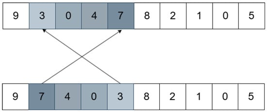
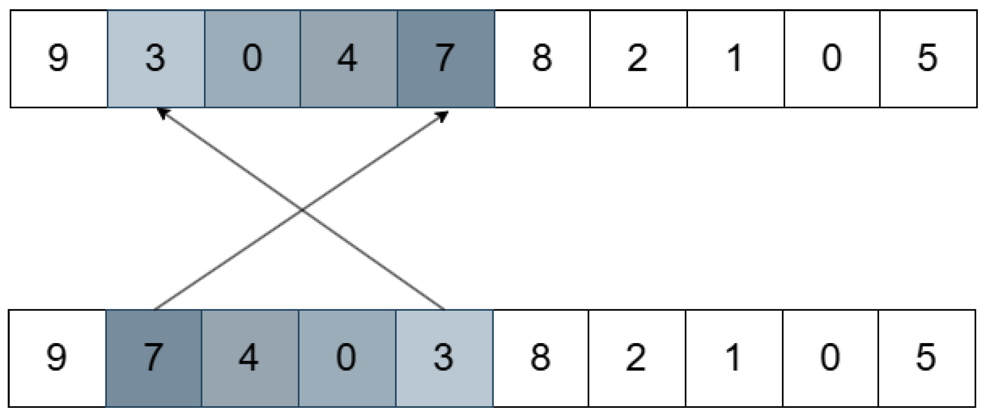
As shown in Figure 4, by swapping the gene segments at 3rd and 6th positions between Route 1: 9-3-8-4-6-7-2-1-0-5 and Route 2: 6-3-0-4-7-8-9-5-1-2, we generate two initial offspring. Offspring 1 becomes: 9-3-0-4-7-8-2-1-0-5, and Offspring 2 becomes: 6-3-8-4-6-7-9-5-1-2.

Next, we perform a duplicate gene correction. The algorithm scans the unexchanged gene segments to identify any duplicates. Then, by mapping the genes between the two offspring, it finds the missing genes and replaces the duplicates with them. Essentially, the offspring inherit the structural framework of the parent routes, while a random portion of the gene sequence is altered.

4.5. Greedy 2-opt Operator

The 2-opt perturbation operator randomly swaps the positions of two request points on a path, retains the original link order, and explores a new solution through a weak perturbation operation. Building upon this, we propose a greedy 2-opt operator, which persistently applies such subtle perturbations along this exploration pattern until a local optimum is reached. A maximum number of 2-opt swaps is predefined, and the loop terminates only when no improved solution is found after exhausting this maximum number of swaps. This approach accelerates the identification of local optima, while subsequent operators facilitate escaping from these local optima, thereby accelerating overall convergence speed.

4.6. Adaptive Local Search Strategy

We improve the local exploration ability in the third stage of the IHTF by introducing an adaptive local search strategy. This enhances the algorithm’s ability to explore the local search space and improves the quality of the solutions. To avoid investing excessive computational resources in local optima early in the search, we design an adaptive strategy with a flexible number of destruction-repair operations (1 to 5). In the early stages, the focus is on convergence speed and exploration breadth, with at least one destruction-repair operation performed. In later stages, we invest more computational cost in local development, allowing up to five destruction-repair iterations, which may slow the search speed.

First, we use the destruction operator to remove several customers from the current route, then apply the repair operator to reintegrate these removed customers into the damaged solution and reconstruct the route.

Destruction operation: Let M represent the set of customers to be removed, and P denote the number of customers to be deleted. First, we randomly select a customer from the original set and add it to M as the first element. Then, the remaining $(P-1)$ elements each randomly select a customer C from M, and we calculate the correlation between the remaining customers in the original solution and C. The customer with the highest correlation to C is then added to M. This process is repeated until $(P-1)$1 customers are selected. The correlation is calculated using the following formula:

$$\begin{array}{c}\hfill R_{ij}={\displaystyle \frac{1}{C+V}}\end{array}$$

(26)

$$\begin{array}{c}\hfill C={\displaystyle \frac{d}{md}}\end{array}$$

(27)

where, $R_{ij}$ represents the correlation between customer i and customer j, d is the distance between customer i and customer j, $md$ is the maximum distance between customer i and any other customer, V is an indicator function where $V=0$ if customers i and j are on the same route, and $V=1$ otherwise. This means that the closer two customers are geographically, the higher their correlation when on the same route.

Repair operation: For each customer removed, we calculate the optimal insertion position in the damaged solution, aiming to minimize the decrease in the fitness function caused by reinserting the customer. We then insert the customers in the order of decreasing fitness improvement. After the local search, if the fitness increases, we update the solution. Otherwise, the new solution is discarded.

4.7. Escape Mechanism

As a metaheuristic algorithm, the IHTF inevitably faces the risk of converging to local optima, which is a critical factor affecting its performance and solution quality. To address this, our study integrates a mutation operator from GA. When a hippo individual is detected as trapped in a local optimum, an escape mechanism is activated to stimulate it to jump out of the local trap.

While the mutation operator possesses considerable perturbation capability, its high randomness and lack of controllability may lead to computational waste. The Metropolis criterion from SA effectively compensates for the short-sightedness of the mutation operator. Mutation introduces variation into the population by altering the genetic material of offspring. Specifically, when a hippo gets trapped in a local optimum, we generate two random numbers at its gene position (regenerated if identical). These numbers correspond to the gene locations to be swapped, creating a new mutated individual. This process is repeated multiple times, as illustrated in Figure 5.

Simultaneously, each mutated individual is accepted based on the Metropolis criterion. After mutation from the old solution to a new one, if the fitness of the new solution j is better than that of the old solution i, the new one j is accepted as the current solution. Otherwise, state j is accepted with a probability $exp[-{\displaystyle \frac{E_j-E_i}{kT}}]$, where $E_j-E_i$ is the fitness difference, k is the Boltzmann constant, and T is the current temperature.The newly interpreted transition probability is

$$\begin{array}{c}\hfill p=\left\{\begin{array}{cc}1\hfill & \mathrm{if}f\left(X_j\right)<f\left(x_i\right)\hfill \\ exp\left(-{\displaystyle \frac{f\left(X_j\right)-f\left(x_i\right)}{T}}\right)\hfill & \mathrm{if}f\left(X_j\right)\ge f\left(x_i\right)\hfill \end{array}\right..\end{array}$$

(28)

4.8. Complexity Analysis of the IHTF Algorithm

In analyzing the time and space complexity of the IHTF algorithm, we consider the main steps of the algorithm, including initial solution generation, fitness function calculation, hippo population position updating, defense operation, and escape operation. The complexity analysis for each step is detailed below:

(1) The initial solution generation uses a chaotic mapping-based random generation algorithm. The chaotic mapping generates n random sequences in one traversal, and then traverses n customers twice to find and replace duplicate numbers. This process repeats POP times, where POP denotes the population size. Therefore, the total time complexity is O(N × POP), and the space complexity is also O(N × POP).

(2) The calculation of the fitness function involves summing multiple cost components and performing numerical computations, which require traversing the entire population of size POP to evaluate the fitness of each individual. By traversing the n-customer sequence of each individual, splitting the delivery sequence into feasible routes under constraints, and computing each cost term using day-ahead prediction information from the forecasting module, the time complexity is O(N × POP). The space complexity is O(N × POP).

(3) The hippo population position updating phase consists of three operators: Cauchy mutation-based hippo movement, improved partially matched operation, and random hippo movement. The Cauchy mutation-based movement traverses the current individual and moves it toward the global optimal individual with Cauchy probability, yielding a time complexity of O(N). The improved partially matched operator swaps gene segments between the current hippo and the optimal hippo, and then replaces duplicate genes via two traversals of the parents through mapping matching, resulting in a time complexity of O(N). The random hippo movement generates a random hippo individual directly, with a time complexity of O(N). Thus, the time complexity of this phase is O(N), and the space complexity is O(N).

(4) The defense phase of the hippo population is composed of discrete hippo movement and the greedy 2-opt operator. Discrete movement drives the hippo individual toward the generated predator to inherit excellent gene segments from the predator, with a time complexity of O(N). The greedy 2-opt operator performs 2-opt searches with an adaptive number of exchanges, up to 10 times, so its time complexity is O(N). In terms of space complexity, it is O(N), which is mainly used to store paths and intermediate results.

(5) The escape phase of the hippo population includes an adaptive VNS operator and an escape mechanism. The VNS operator consists of destruction and reconstruction procedures, both of which require double traversals to find the optimal positions, leading to a time complexity of O(N2). The escape mechanism accepts inversion mutation results under the Metropolis criterion for a maximum of 30 iterations, and the time complexity of inversion mutation is O(N). The space complexity is O(N).

Based on the above analysis, the time complexity of the IHTF algorithm is dominated by the fitness function calculation and the VNS operator in the escape phase, giving an overall time complexity of O(N2). The space complexity is mainly used to store paths, individuals, and intermediate results, resulting in an overall space complexity of O(N).

5. Experimental Results and Analysis

To demonstrate the effectiveness of IHTF for solving the VRPTW, we evaluate the performance of the proposed approach using Python 3.7.5 and PyTorch 1.3.0 on a desktop computer equipped with a 6-core Intel i5-12500H CPU and 16 GB of RAM. Meanwhile, this paper conducts simulation experiments on both the Solomon benchmark dataset and a simulation dataset integrated with real road networks. The Solomon dataset provides detailed instance information, including instance names, customer locations, service time windows, customer demand volumes, vehicle capacity constraints, and the maximum fleet size. The instances are categorized into three types: R-type, where node coordinates are randomly generated and widely dispersed; C-type, where node coordinates form distinct geographic clusters; and RC-type, which combines random and clustered patterns. The depot time window is set to 0–1236 min for all instance types. The simulation dataset is derived from a 10 × 10 km area in Luohu District, Shenzhen. Weather conditions, POI attributes, and weekday labels are obtained from Chinese meteorological websites, map services, and calendar data. We also generate 100 customer locations at random; the distances between customers correspond to real road distances retrieved from Baidu Maps. Each customer’s service window and service duration are generated randomly.

5.1. Prediction Performance of STD-RND

To verify the performance of the STD-RND module, we test its performance multiple times over 500 time steps on a real dataset. The parameter settings are as follows: the learning rate, batch size, and training-test set split ratio are set to 0.001, 64, and 0.8, respectively; the number of training epochs is 3000, and the number of hidden units is 100. We finally select the ADAM optimizer to train the STD-RND model. Meanwhile, this paper adopts 5-fold cross-validation and repeats the model training and testing process; in addition, the experimental results of each cross-validation fold are independently repeated 5 times, and the average value is taken. We ultimately obtain the overall performance of the model by synthesizing the results of the 5-fold validation.

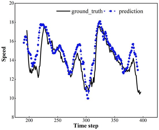
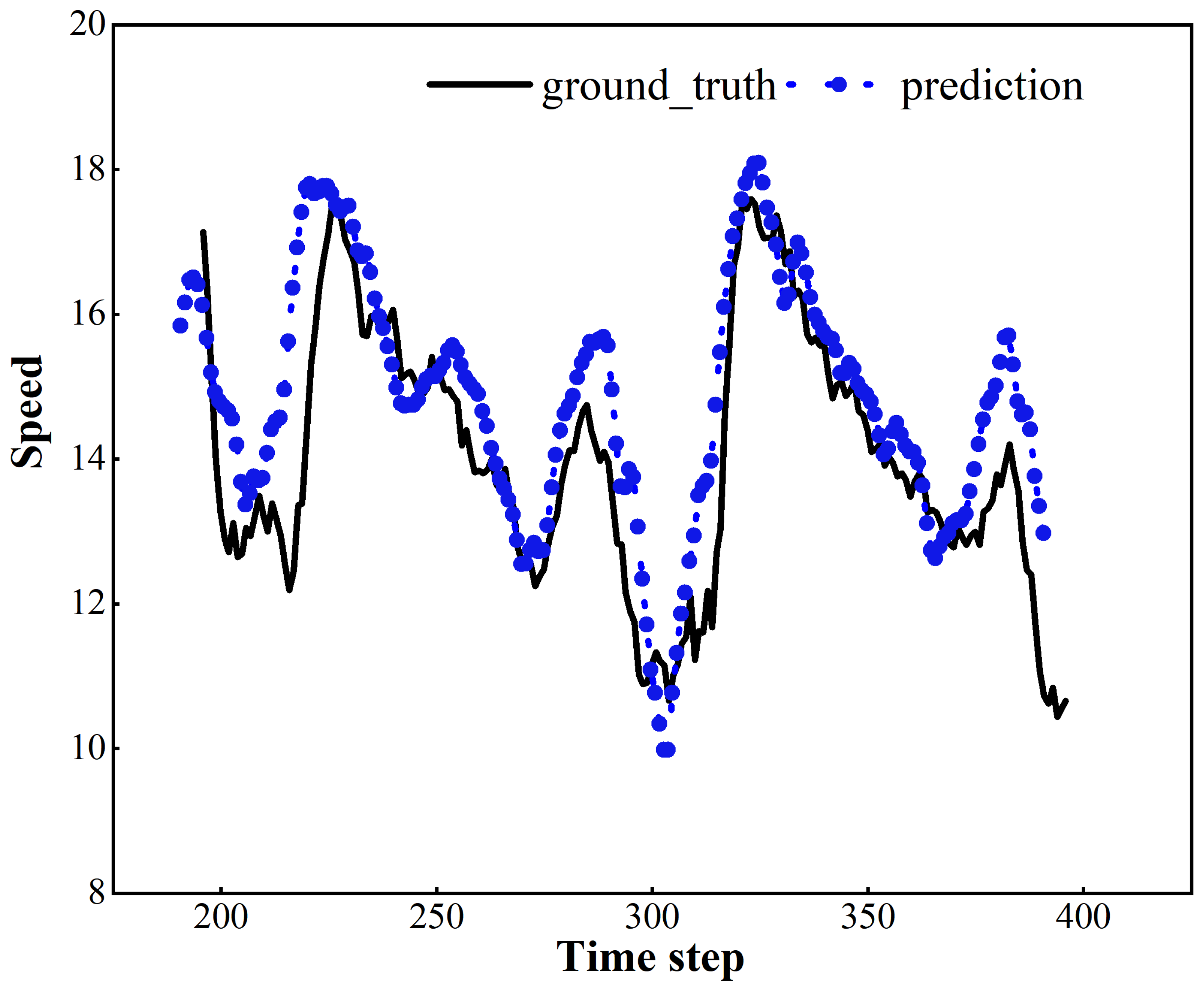
As shown in Figure 6, the average prediction accuracy of the proposed STD-RND prediction module reaches $80\%\pm 2.27$, verifying the effectiveness and stability of the module.

At the same time, we conducted comparative experiments on a real dataset with a time granularity of 15 min in the real world over 500 time steps to test its performance. We compare STD-RND against several baseline models using prediction accuracy, MAE (Mean Absolute Error), RMSE (Root Mean Square Error), and MAPE (Mean Absolute Percentage Error): (1) ARIMA (AutoRegressive Integrated Moving Average), which fits the observed time series to a parametric model for forecasting; (2) GCN (Graph Convolutional Network); (3) GRU (Gated Recurrent Unit); (4) T-GCN (Temporal Graph Convolutional Network).

The results in

Table 2. Comparison of different models.

Model	Accuracy	MAE	RMSE	MAPE
ARIMA	0.4782	6.1544	8.0943	0.2315
GCN	0.6785	6.9172	8.9351	0.2584
GRU	0.7145	2.7431	4.3827	0.1968
T_GCN	0.7574	2.7059	3.8462	0.1874
STD-RND	0.8062	2.5143	3.7548	0.1757

show that STD-RND reaches 80% accuracy on the current dataset and achieves the best scores across all error metrics.

The comparison highlights three key observations: Models that incorporate temporal feature modeling outperform parametric models like ARIMA, because ARIMA struggles with highly volatile and non-smooth time series. The comparison STD-RND and T-GCN with the standalone GRU model shows that spatial correlations in traffic flow significantly influence prediction accuracy. The comparison between STD-RND and T-GCN demonstrates that learning latent external features through a multi-head attention mechanism effectively enhances prediction performance.

5.2. Experimental Analysis of IHTF on Real Road Networks

To evaluate the performance of the Improved Hippopotamus Optimization Algorithm with Traffic Forecasting (IHTF), this paper compares it with the Student Psychology based Ant Colony Optimization hybrid algorithm (SP_ACO) [27] and the Immune Affinity Particle Swarm Optimization hybrid algorithm (IA_PSO) [28] on the aforementioned real road network dataset. We run each algorithm 10 times and take the average value to compare their convergence performance across iterations. We also use an ablated version of IHTF to verify the effectiveness of the improvement strategies proposed in this work. The population size of all algorithms is uniformly set to 100, and the solution dimension is set to 100. In IHTF and its ablated variant, the crossover coefficient is fixed at 0.85, the mutation coefficient at 0.02. The jumping coefficient m was determined through a grid search within the range [0.1, 0.2, 0.3, 0.4, 0.5], and it was found that m = 0.2 allows the algorithm to achieve faster convergence and better solution quality. All algorithms adopt a fixed random seed of 64. Those algorithms in this study uses unified cost parameters: $c_1=400\mathrm{CNY}/\mathrm{t}$, $c_2=20\mathrm{CNY}/\mathrm{km}$, $c_3=15\mathrm{CNY}/\mathrm{KJ}$, $c_4=0.5\mathrm{CNY}/\mathrm{kg}$, $P_{\phi }=60\mathrm{CNY}/\mathrm{t}$, $P_{\eta }=180\mathrm{CNY}/\mathrm{t}$, which are set and reasonably adjusted based on existing literature and experimental results. SP_ACO and IA_PSO use the classic parameter settings widely accepted in related literature to maintain consistency with existing works and ensure fair experimental comparisons.

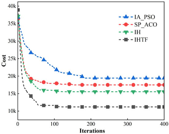
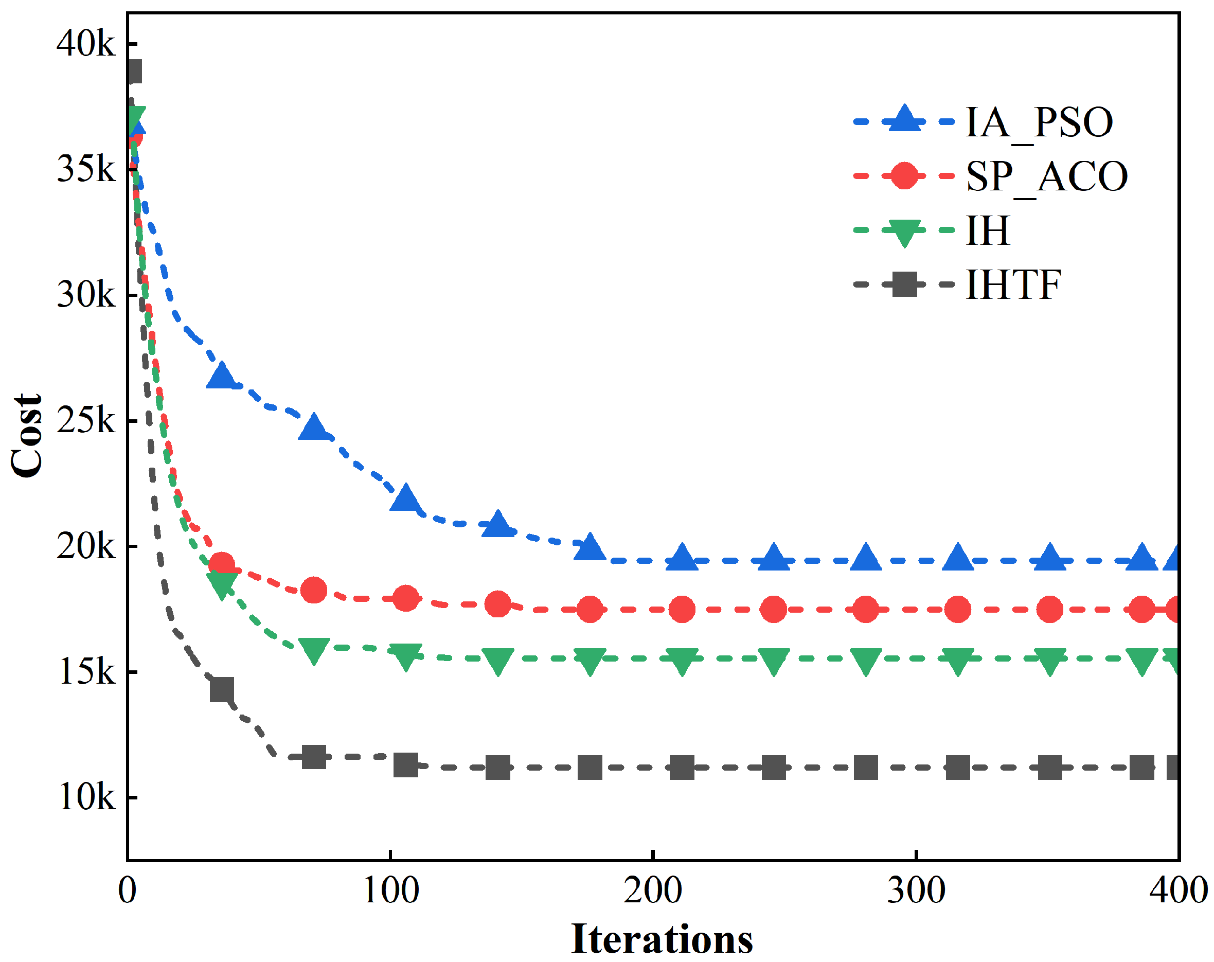
We run all four algorithms repeatedly on the real road network data and conduct a statistical analysis of their results. Figure 7 shows the average convergence curves from iteration 0 to 400. IHTF clearly outperforms the other two classical hybrid algorithms in both convergence speed and solution quality. This demonstrates that combining the global search framework of HO with adaptive local search, escape mechanisms, and hybrid operators successfully addresses the VRPTW.

We also observe that IHTF achieves significantly better convergence quality than the other three algorithms without prediction modules. This confirms that integrating traffic forecasting to proactively avoid congestion dramatically reduces overall cost. These results verify the effectiveness of both the proposed IHTF improvement strategies and the traffic-prediction module (STD-RND) in solving time-dependent VRPTW.

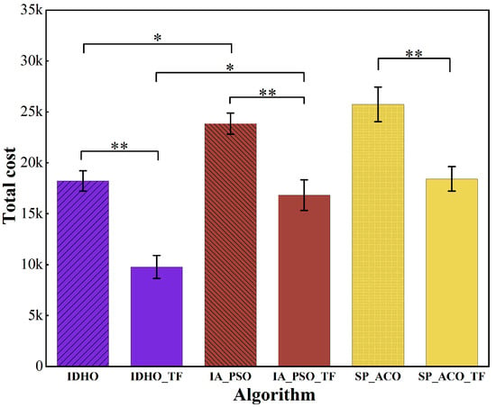
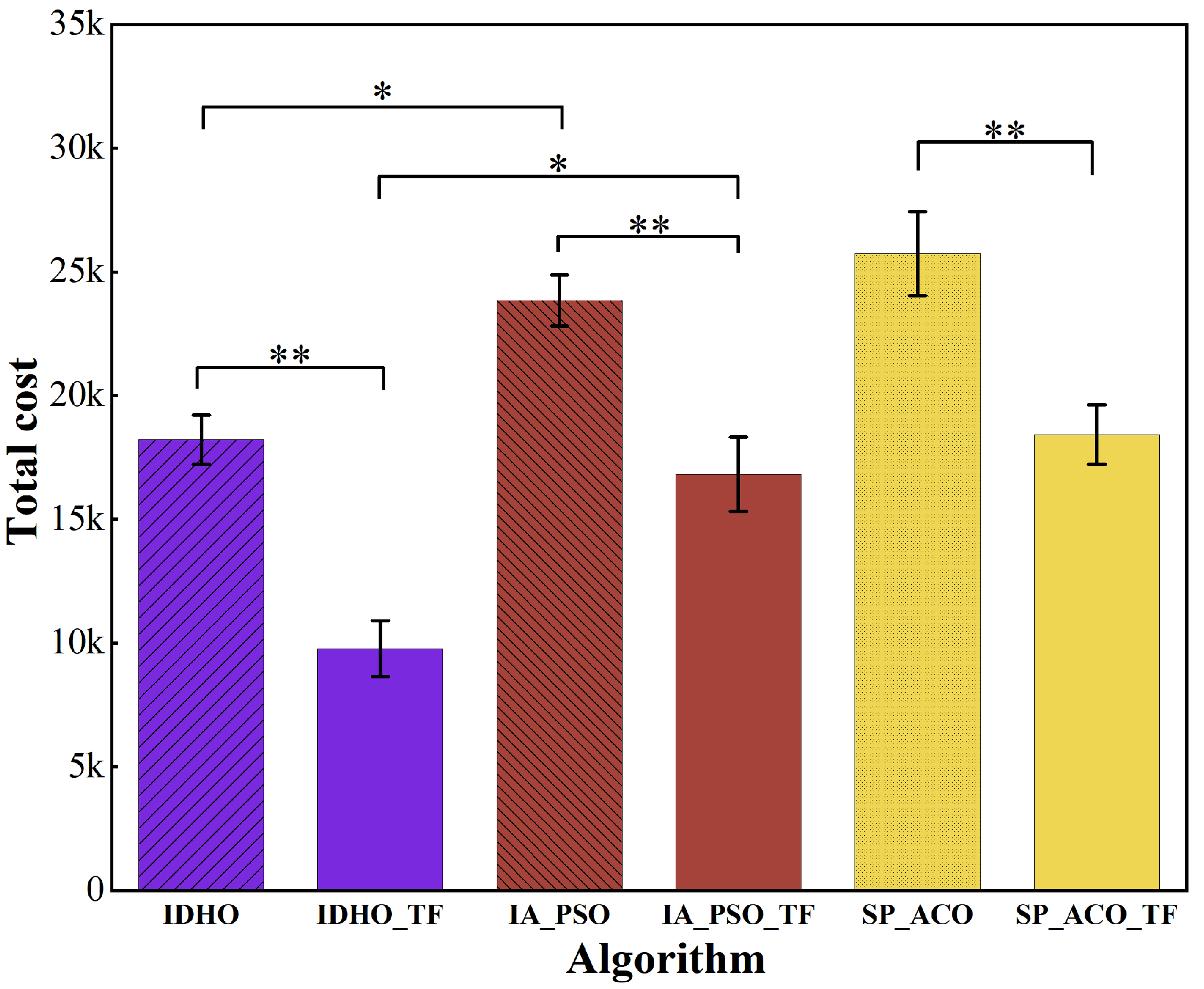
Next, we embed the STD-RND prediction module into the comparison algorithms to further validate the feasibility of combining deep learning-based traffic forecasting with IHTF optimization for cold chain time-dependent VRP: (1) IA_PSO_TF (IA_PSO integrated with traffic forecasting); (2) SP_ACO_TF (SP_ACO integrated with traffic forecasting). We compare these two variants and the three original algorithms on a delivery case constructed using real road data from Luohu District, Shenzhen. In this scenario, this paper constructs 100 merchant nodes on real roads to create the experimental instances and conducts 10 independent experiments, with the results shown in Figure 8.

Across all test cases, IHTF achieves the lowest total cost, outperforming both hybrid variants and the original IH algorithm. Adding the prediction module consistently improves IHTF performance. The ablation study further shows that, even without the prediction module, the adaptive local search and escape mechanisms significantly enhance IHTF’s solution quality and exploration capability.

5.3. Performance of IHTF on the Solomon Dataset

To compare the effectiveness and applicability of the improvement strategies in the IHTF optimization algorithm, we contrast its performance with that of comparative algorithms and the known best solutions (BKS) of the Solomon benchmark instances on standard VRPTW metrics across the benchmark instances C101, R101, and RC101, including total travel distance(TD), number of vehicles used(VN), total computation time(TT), and total cost(TC). The algorithm runs 10 times on each instance, with the average value and standard deviation calculated for the results. The results are presented in the

Table 3. Classic performance metrics of three algorithms on different instances of the Solomon dataset, where - indicates the Best-known solutions of Solomon benchmark instances do not discuss the relevant metrics.

	C101				R101				RC101
	VN	TD	TT	TC	VN	TD	TT	TC	VN	TD	TT	TC
SP_ACO	13	884.1	0.51	4420.5 + 80.4	21	1724.3	0.77	3165.5 + 65.7	15	1765.4	0.87	3827.7 + 73.4
IA_PSO	12	873.2	0.48	4196.1 + 65.7	20	1703.4	0.75	2567.5 + 54.6	15	1744.9	0.86	3460.1 + 45.6
IHTF	10	834.5	0.42	3795.5 + 21.8	19	1673.8	0.69	2997.3 + 19.8	14	1702.9	0.78	3220.7 + 25.2
BKS	10	828.9	-	-	19	1650.8	-	-	14	1696.5	-	-

.

The table above demonstrates the superior performance and good portability of the proposed IHTF in addressing such classic VRPTW problems. To verify the reliability of the experimental results obtained by the three algorithms, we conduct a statistical significance test on the total cost data for each instance. Prior to the significance test, a normality test is first performed. The results indicate that some data do not satisfy the normal distribution assumption; thus, the Kruskal–Wallis H test is adopted. At a significance level of $\alpha$ = 0.05, the non-parametric test yields three p-values ($p_1=4.7\times {10}^{-9},p_2=3.6\times {10}^{-9},$$p_3=5.3\times {10}^{-9}$), all of which are less than 0.05. This indicates that IHTF is significantly superior to other algorithms in experimental results, while the results are extremely close to the published optimal values, and the differences are statistically significant.

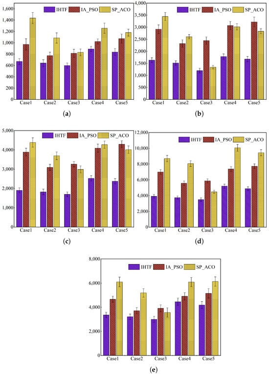
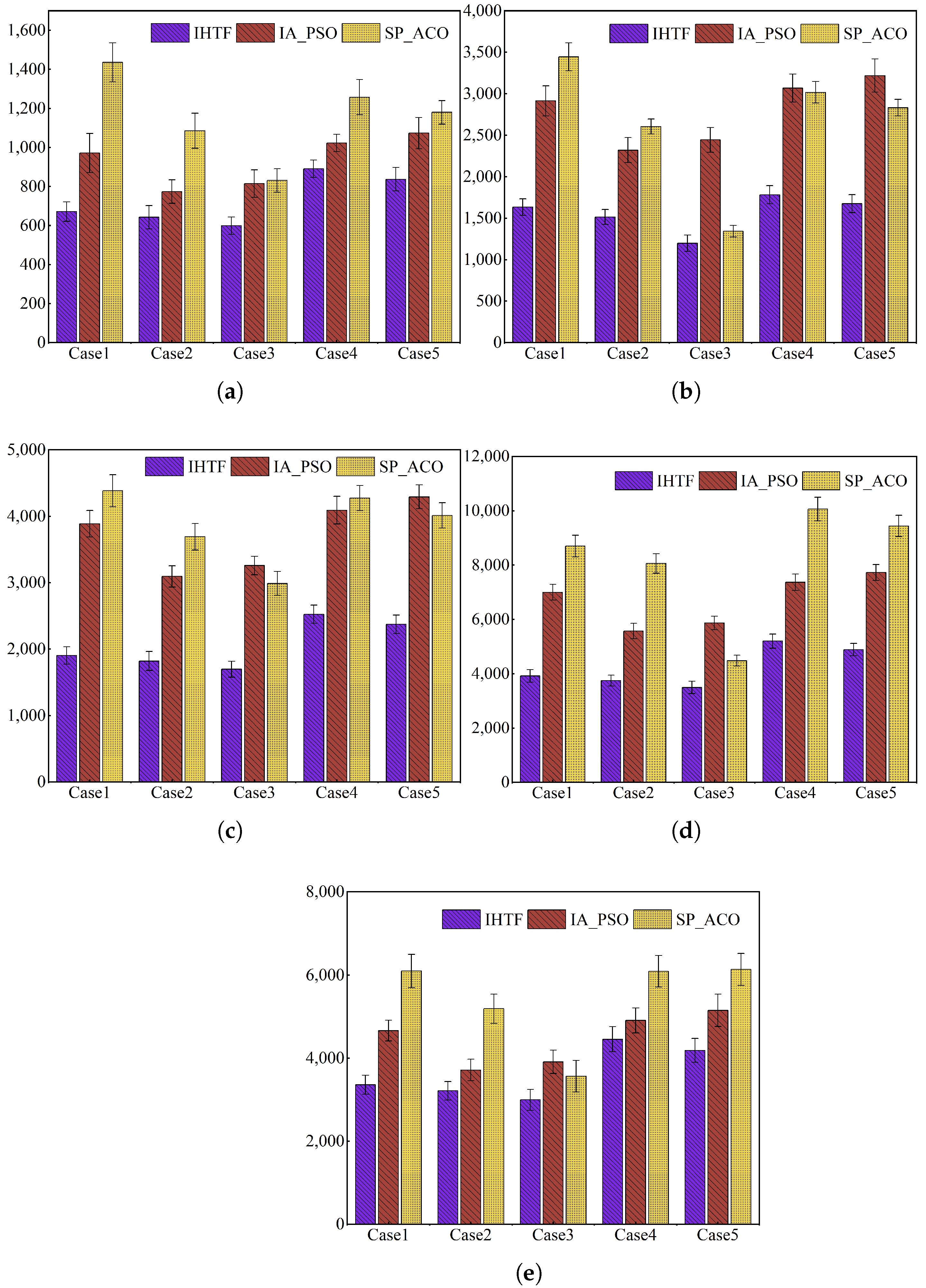
To evaluate the effectiveness of the IHTF optimization algorithm in practical cold-chain applications and its exploration ability on different cost components, we randomly select 5 instances from each of the three categories in the Solomon dataset and perform 10 independent repeated experiments. We compare the three algorithms in terms of travel distance, refrigeration cost, carbon emission cost, flower spoilage cost, and time-window penalty cost.

As shown in Figure 9, although SP_ACO and IA_PSO already perform well, IHTF consistently outperforms them across all cost metrics. This advantage comes from both IH’s intrinsic strengths its movement strategy and predator avoidance mechanism that grant it strong exploration ability and the improvements introduced in IH. The adaptive local search strategy broadens exploration, while the escape mechanism helps the algorithm break free from local optima.

6. Conclusions and Look Forward

This paper presents a comprehensive study of the IHTF algorithm for the VRPTW, with an emphasis on minimizing distribution costs by integrating real-traffic prediction and an enhanced optimization framework. We analyze the effectiveness of the combined modules and algorithmic strategies, and we show that the proposed method delivers superior solution quality and stability, especially in scenarios with uncertain road conditions or large-scale problem instances.

Future research will consider additional realistic constraints and multi-objective formulations. We also plan to incorporate driver-behavior modeling and product heterogeneity into the solution framework, making the approach not only theoretically sound but also practically useful for real-world logistics.

Furthermore, we aim to explore the integration of deep reinforcement learning to autonomously learn traffic conditions and assist swarm intelligence algorithms in route planning. This will enhance the system’s ability to learn complex patterns beyond traditional mathematical structures, offering a promising and practical direction for cold-chain logistics under realistic operational conditions.

References

- Lu, M.; Wang, S. An improved spider wasp optimizer for green vehicle route planning in flower collection. Appl. Sci. 2025, 15, 4992. [Google Scholar] [CrossRef] [Scilit]
- Zheng, F.; Pang, Y.; Xu, Y.; Liu, M. Heuristic algorithms for truck scheduling of cross-docking operations in cold-chain logistics. Int. J. Prod. Res. 2021, 59, 6579–6600. [Google Scholar] [CrossRef] [Scilit]
- Yang, F.; Tao, F. A bi-objective optimization VRP model for cold chain logistics: Enhancing cost efficiency and customer satisfaction. IEEE Access 2023, 11, 127043–127056. [Google Scholar] [CrossRef] [Scilit]
- Jia, Y.H.; Mei, Y.; Zhang, M. A bilevel ant colony optimization algorithm for capacitated electric vehicle routing problem. IEEE Trans. Cybern. 2021, 52, 10855–10868. [Google Scholar] [CrossRef] [Scilit]
- Zhang, X.; Hao, Y.; Zhang, L.; Yuan, X. Application of improved genetic algorithm to vehicle routing problem considering the environmental self-regulation of the freight companies. Expert Syst. Appl. 2025, 274, 127010. [Google Scholar] [CrossRef] [Scilit]
- Tronconi, R.; Pilati, F. Social, economic and green optimization of the distribution process of e-commerce platforms. Transp. Res. Part E Logist. Transp. Rev. 2025, 196, 104004. [Google Scholar] [CrossRef] [Scilit]
- Ma, Z.; Jen, C.T.; Aazami, A. Time-Dependent Vehicle Routing Optimization Incorporating Pollution Reduction Using Hybrid Gray Wolf Optimizer and Neural Networks. Sustainability 2025, 17, 4829. [Google Scholar] [CrossRef] [Scilit]
- Ren, C.; Lu, L.; Teng, J.; Yin, C.; Li, J.; Ji, H.; Wang, X.; Fu, F. Logistics Distribution Path Optimization Considering Carbon Emissions and Multifuel-Type Vehicles. J. Adv. Transp. 2025, 2025, 6668589. [Google Scholar] [CrossRef] [Scilit]
- Zhang, J.; Li, Y. Vehicle routing problem for cold-chain drug distribution with epidemic spread situation. Expert Syst. Appl. 2025, 262, 125186. [Google Scholar] [CrossRef] [Scilit]
- Liu, H.; Zhang, J.; Dai, Y.; Qin, L.; Zhi, Y. Multi-constraint distributed terminal distribution path planning for fresh agricultural products. Appl. Intell. 2025, 55, 180. [Google Scholar] [CrossRef] [Scilit]
- Jiang, X.; Liu, X.; Pan, F.; Han, Z. Optimizing cold chain distribution routes considering dynamic demand: A low-emission perspective. Sustainability 2024, 16, 2013. [Google Scholar] [CrossRef] [Scilit]
- Iksan, N.; Tufail, A.; Apong, R.A.; Hidayatullah, A.F. Optimizing maritime passenger transfer in rich vehicle routing problem using a hybrid genetic algorithm. IEEE Access 2024, 12, 80153–80164. [Google Scholar] [CrossRef] [Scilit]
- Frías, N.; Johnson, F.; Valle, C. Hybrid algorithms for energy minimizing vehicle routing problem: Integrating clusterization and ant colony optimization. IEEE Access 2023, 11, 125800–125821. [Google Scholar] [CrossRef] [Scilit]
- Vrani, A.; Apostolidis, S.D.; Kapoutsis, A.C.; Kosmatopoulos, E.B. Delivering data: A real-world dataset for last-mile delivery optimization. Data Brief 2025, 61, 111762. [Google Scholar] [CrossRef] [Scilit] [PubMed]
- Akkerman, F.; Mes, M.; van Jaarsveld, W. A comparison of reinforcement learning policies for dynamic vehicle routing problems with stochastic customer requests. Comput. Ind. Eng. 2025, 200, 110747. [Google Scholar] [CrossRef] [Scilit]
- Heidari, R.; Ghazanfari, M.; Rasouli, M.R. A decision support system for resilient vehicle route planning using mathematical modeling and artificial neural networks: A case study. Kybernetes 2024, 55, 944–964. [Google Scholar] [CrossRef] [Scilit]
- Sze, J.F.; Salhi, S.; Wassan, N. An adaptive variable neighbourhood search approach for the dynamic vehicle routing problem. Comput. Oper. Res. 2024, 164, 106531. [Google Scholar] [CrossRef] [Scilit]
- Patil, M.; Tambolkar, P.; Midlam-Mohler, S. Optimizing Traffic Routes with Enhanced Double Q-Learning. IET Intell. Transp. Syst. 2025, 19, e70002. [Google Scholar] [CrossRef] [Scilit]
- Nyako, S.I.; Tayachi, D.; Abdelaziz, F.B. Machine learning multi-objective optimization for time-dependent green vehicle routing problem. Energy Econ. 2025, 148, 108628. [Google Scholar] [CrossRef] [Scilit]
- Xidias, E.; Zacharia, P.; Nearchou, A. Intelligent fleet management of autonomous vehicles for city logistics. Appl. Intell. 2022, 52, 18030–18048. [Google Scholar] [CrossRef] [Scilit]
- Nisyrios, E.; Gkiotsalitis, K. Optimization-based approaches for traffic and fleet management of connected and autonomous vehicles: A systematic literature review. Int. J. Intell. Transp. Syst. Res. 2025, 23, 1–23. [Google Scholar] [CrossRef] [Scilit]
- Xue, H. Adaptive Cultural Algorithm-Based Cuckoo Search for Time-Dependent Vehicle Routing Problem with Stochastic Customers Using Adaptive Fractional Kalman Speed Prediction. Math. Probl. Eng. 2020, 2020, 7258780. [Google Scholar] [CrossRef] [Scilit]
- Liu, Y.; Zhao, S.; Guan, F.; Yuan, Y. Establishment of a model for evaluating shelf life of Pseudosciaena crocea in simulated logistics and storage. J. Food Prot. 2021, 84, 1188–1193. [Google Scholar] [CrossRef] [Scilit]
- Xiao, Y.; Zhao, Q.; Kaku, I.; Xu, Y. Development of a fuel consumption optimization model for the capacitated vehicle routing problem. Comput. Oper. Res. 2012, 39, 1419–1431. [Google Scholar] [CrossRef] [Scilit]
- Liu, C.; Kou, G.; Zhou, X.; Peng, Y.; Sheng, H.; Alsaadi, F.E. Time-dependent vehicle routing problem with time windows of city logistics with a congestion avoidance approach. Knowl.-Based Syst. 2020, 188, 104813. [Google Scholar] [CrossRef] [Scilit]
- Amiri, M.H.; Mehrabi Hashjin, N.; Montazeri, M.; Mirjalili, S.; Khodadadi, N. Hippopotamus optimization algorithm: A novel nature-inspired optimization algorithm. Sci. Rep. 2024, 14, 5032. [Google Scholar] [CrossRef] [Scilit]
- Wei, X.; Niu, C.; Zhao, L.; Wang, Y. Combination of ant colony and student psychology based optimization for the multi-depot electric vehicle routing problem with time windows. Clust. Comput. 2025, 28, 99. [Google Scholar] [CrossRef] [Scilit]
- Leng, K.; Li, S. Distribution path optimization for intelligent logistics vehicles of urban rail transportation using VRP optimization model. IEEE Trans. Intell. Transp. Syst. 2021, 23, 1661–1669. [Google Scholar] [CrossRef] [Scilit]
Disclaimer/Publisher’s Note: The statements, opinions and data contained in all publications are solely those of the individual author(s) and contributor(s) and not of MDPI and/or the editor(s). MDPI and/or the editor(s) disclaim responsibility for any injury to people or property resulting from any ideas, methods, instructions or products referred to in the content. |
© 2026 by the authors. Licensee MDPI, Basel, Switzerland. This article is an open access article distributed under the terms and conditions of the Creative Commons Attribution (CC BY) license.