Discrete Body Dynamics: A Numerical Method for Multibody Systems Investigated on Closed-Chain Problems

Abstract

Discrete Body Dynamics (DBD) is a recently developed approach for solving multibody dynamics problems that aims to improve the numerical treatment of systems with joint compliance. Conventional multibody formulations typically rely on kinematic constraints, which can increase numerical complexity and sensitivity, particularly in closed-chain systems. In this work, DBD is presented as a unified framework that combines a new modeling approach with a new numerical solution strategy. Mechanical joints are modeled explicitly using sets of springs and dampers, replacing ideal constraints and transforming the governing equations from a differential-algebraic system into a purely differential one. Based on this modeling framework, the numerical solution avoids global matrix operations and relies on element-wise computations, resulting in linear computational complexity with respect to the number of bodies. The numerical performance of the DBD method is investigated using a set of closed-chain benchmark systems, which are known to be challenging for conventional constraint-based solvers. The analysis examines the influence of joint stiffness, system dynamics, time-step selection, and mechanism topology on numerical stability, energy dissipation, and computational efficiency. The results show that DBD maintains robust and accurate solutions across the examined scenarios and exhibits a well-defined operating region with low numerical dissipation. Across the examined compliant-joint benchmarks, DBD shows the potential for up to three orders of magnitude lower energy drift at comparable simulation-time-to-real-world time (SRT), or up to about one order of magnitude higher SRT at comparable energy drift, relative to ADAMS/View. These findings indicate that DBD is well suited for the simulation of realistic multibody systems with compliant joints, including closed-chain configurations.

1. Introduction

Closed-chain multibody systems comprise interconnected rigid bodies that form a closed loop. These systems are commonly used in various fields, such as robotic manipulators, biomechanics, and automotive engineering. However, due to their complexity, analyzing and comprehending the dynamics of these systems can be challenging [1]. Nonetheless, understanding their dynamics is critical for designing, controlling, and simulating the behavior of complex systems.

Among the more commonly used components in closed-chain systems are the four-bar mechanism, the five-bar mechanism, the 3RRR mechanism, and the 3RUU mechanism (delta robot), which comprise rigid components such as linkages and cranks, as well as joints such as revolute and universal. Understanding the dynamics of these mechanisms is necessary to comprehend the behavior of closed-chain multibody systems and to optimize their design dynamics.

It is essential to solve the dynamics of closed-chain systems to optimize the design and understand their behavior. Various methods can be used for this purpose, each with its own advantages and disadvantages. One of the most used methods for dynamics analysis is the Lagrangian method. This method employs Lagrangian mechanics to derive the equations of motion for each body in the system, providing a clear physical interpretation of the equations. However, the equations of motion derived using Lagrangian dynamics can exhibit high levels of complexity and nonlinearity, particularly when dealing with mechanical systems that include closed-chain and parallel mechanisms. As a result, solving systems with closed-chain and parallel mechanisms can require significant computational effort, which can be a drawback in terms of systematization and implementation in computer algorithms. This difficulty arises due to the use of a minimal number of generalized independent coordinates, which results in complex and nonlinear relations when expressing the center of mass coordinates and velocity in terms of generalized independent coordinates [1]. To address this issue, several methods have been developed that involve cutting the closed chain into several open loops, such as Lagrangian with cut joint [2], Lagrangian with clearance joint [2], and Lagrangian with elastic joint [1]. However, these methods also have their challenges. For example, the Lagrangian with the cut joint method may violate constraint equations during numerical resolution, while the Lagrangian with the clearance joint method can encounter numerical difficulties with small clearance sizes [1]. All these methods involve differential-algebraic equations (DAEs), which may suffer from loss of accuracy with changes in step size or integration order, leading to errors in the algebraic variable [3]. The Lagrangian with the elastic joint method can also introduce numerical instability with high stiff spring constants and has a high variation in mechanical energy during simulation. While all of these methods have difficulties in the development of a general-purpose program, none of them have been identified as superior to the others [1].

Malak [4] simulated the four-bar mechanism based on the Lagrangian formulations previously proposed in [5]. The simulation was built using SimMechanics and Matlab code. However, the development of the equations is not straightforward and includes some assumptions that may introduce inaccuracies to the model.

Kane’s method is another dynamics analysis approach based on the principle of virtual work. It can handle systems with nonlinear constraints and is computationally efficient, making it advantageous for some applications. However, it requires a good understanding of the system’s kinematics and may not be suitable for highly complex systems [6].

The recursive Newton-Euler method (RNE) is another widely used approach for dynamics analysis. This method employs Newton’s second law and Euler’s equations to calculate the forces and torques acting on each body. It is computationally efficient and can handle systems with high degrees of freedom for open-loop robots. However, for closed-chain robots, there is no recursive method available to obtain the direct dynamic model, so the inertia matrix and the Coriolis, centrifugal, and gravity matrices need to be computed [7]. In parallel robots, the Jacobian matrix and its inverse are required, which can be challenging to obtain for complex systems. Therefore, programming RNE numerically can be challenging, and the complexity may increase to O(n³) as the number of closed chains increases [8]. Where n is the number of equations, which includes both differential and algebraic equations resulting from the number of bodies and constraints. Another drawback of RNE is that the serial calculation may introduce kinematic errors from the body to its neighboring links [9]. Several advanced methods have been developed to handle closed-chain systems more effectively. The fully augmented (FA) method treats all bodies as independent, and constraints are explicitly handled as bilateral constraints [10]. However, this approach results in a system of DAEs requiring a convergence process to manage constraint errors. The tree-augmented (TA) method addresses this by cutting certain constraints and hence converts the close-chain system into an open-loop system [11]. Nonetheless, this method also results in DAEs. Constraint embedding (CE) avoids the DAE formulation by embedding the constraint equations within the connected bodies [12]. This method, however, introduces additional complexity because the aggregated bodies exhibit configuration-dependent geometry [13]. The hybrid closed-chain dynamic algorithm combines the TA and CE approaches, allowing the user to select the most suitable method for each closed-chain constraint in the system [13]. This hybrid method still suffers from the limitations of the RNE algorithm, such as the need for complex calculations and the introduction of kinematic errors from the body to its neighboring links.

The Multibody Dynamics (MBD) method is widely regarded as one of the most accurate approaches for simulating mechanical systems, as it enables simultaneous convergence of both ordinary differential equations (ODEs) and constraint equations [14]. The MBD method is commonly used in general-purpose software, including MSC ADAMS [15], Altair MotionView [16], and Siemens Simcenter [17]. However, due to its high computational complexity, on the order of O(n³), it may not be suitable for control purposes. Additionally, MBD’s reliance on DAEs can introduce inaccuracies [18]. MBD also models friction as a function of relative velocity rather than relative displacement, which can lead to non-physical friction behavior. Despite these limitations, MSC.ADAMS, which employs a DAE-based solver, was chosen as the benchmark reference for this study, as this method is widely regarded as the most accurate approach.

The penalty method [19] eliminates the explicit differential-algebraic structure of constrained multibody systems by replacing ideal kinematic constraints with artificial stiffness and damping forces that act whenever the constraint is violated. Although this reformulation results in an ordinary differential equation (ODE) system, the formulation remains fundamentally constraint-based, as the governing equations still depend on deviations from the underlying ideal constraint structure.

In implicit integration schemes, the nonlinear solution procedure effectively seeks configurations that reduce constraint violations at each time step. Consequently, the penalty parameters primarily serve as numerical enforcement coefficients controlling how strongly these deviations are corrected. Their magnitudes directly influence both the conditioning of the numerical problem and the stability of the time integration. Large penalty factors improve constraint satisfaction but may introduce stiff dynamics and instability, whereas smaller values reduce stiffness at the expense of increased constraint drift.

In closed-chain systems, where multiple constraints interact, these effects become more pronounced. Additional stabilization techniques, such as Baumgarte-type corrections, are frequently introduced to regulate the evolution of constraint errors. As discussed in [20], the solution may be highly sensitive to the selection of penalty factors, and improper tuning can result in either excessive constraint drift or numerical instability. These considerations highlight the inherent trade-off between constraint accuracy and numerical robustness in penalty-based formulations and motivate the exploration of alternative modeling approaches that avoid constraint enforcement at the formulation level.

Another method to avoid DAEs is through velocity partitioning and Lie group integration [21]. However, coordinate partitioning consumes a substantial portion of the time in each simulation step and involves building the Newton iteration matrix along with its LU decomposition. Moreover, the results indicate a drift in total energy.

Despite the progress made in the field of dynamics analysis, there is still no general-purpose method available that can provide accurate and fast solutions for complex closed-chain systems. In our previous work, we have proposed and developed the Discrete Body Dynamics (DBD) method [18]. This method redefines the treatment of joints within the numerical scheme for solving the equation of motion (EOM) and during the convergence process. The core principle of DBD is to represent joints using a set of springs and dampers, thereby eliminating constraints and transforming the problem from a system of DAEs to a purely differential equation system. By utilizing element-wise products rather than matrix operations in both the prediction and the convergence steps, the computational complexity is reduced to O(n).

The DBD method may be well-suited for analyzing systems with joint clearance. Clearance in joints is unavoidable due to manufacturing processes and other practical factors, and it plays a crucial role in the dynamic analysis of high-speed and high-precision mechanisms. While these joints are often idealized as having no clearance, dynamic analyses reveal that clearance significantly impacts system behavior. Studies have shown that factors such as clearance size, lubricant viscosity, and operating conditions influence the stability and dynamic response of these mechanisms [22].

In our prior work, the DBD method was successfully applied to open-loop manipulators with revolute joints [18]. While this method offers a fast and accurate solution, its applicability to closed-loop systems has not been validated, and it was demonstrated with a revolute joint only. Moreover, the spherical, cylindrical, translational, and universal joints, which are commonly used in such systems, were not demonstrated. Furthermore, the limitations of the DBD method in comparison to MBD have not been clearly established, particularly regarding its sensitivity to model complexity and the critical selection of spring-damper parameters for joint representation. This paper aims to address these knowledge gaps.

A recent systematic review by Archut and Corves [23] offers important insight into the requirements for real-time capable multibody simulation of road vehicles, particularly those involving elastokinematic suspensions with bushings. These bushings introduce practical benefits such as vibration isolation and improved handling but also pose numerical challenges due to high stiffness, damping, and closed-loop topologies, which result in numerical stiffness and computational bottlenecks in traditional MBD formulations. The review outlines six key principles for real-time capability, including the elimination of constraints, the use of purely differential formulations, Jacobian-free implementation, parallelizability, and native support for bushings. The proposed DBD method aligns well with these principles: its constraint-free formulation and use of explicit ODE integration naturally bypass Jacobian computation and are well suited for parallel implementation. Its treatment of joints as spring-damper elements parallels the modeling of bushings in vehicle suspensions. Archut and Corves [23] explicitly discuss the DBD method in this context and highlight its compatibility with real-time elastokinematic vehicle models. However, limitations remain: the method relies on explicit integration schemes, which may require small time steps in stiff systems, and the replacement of rigid bodies with compliant elements introduces approximations that may reduce accuracy, especially in the high-frequency domain.

Some of the aforementioned limitations were addressed in our previous work [18], particularly by improving the integration scheme. The remaining challenges are tackled in the present paper, including the generalization of the joint representation to cover all primitive joint types commonly used in multibody systems. Furthermore, the paper addresses the selection and tuning of time step sizes and the appropriate stiffness and damping values of the virtual springs and dampers used in the DBD formulation.

In closed-chain systems, the reviewed approaches can be summarized as follows:

Lagrangian/Kane formulations (including cut/clearance/elastic variants): systematic equation derivation with a clear modeling framework; however, closed loops typically lead to DAE models with complex nonlinear relations and require explicit constraint handling/stabilization. Reported drawbacks include constraint violation (cut-joint), numerical difficulties for small clearances, sensitivity to step size/integration order in DAEs, and stiffness-related instability/energy variation when elastic joints are used.

RNE-based closed-chain algorithms (including FA/TA/CE and hybrids): applicable to closed loops via loop-closure treatment; however, they require Jacobian-related computations and iterative procedures, the computational burden can grow substantially with closed-chain complexity (often reported as $O\left(n^3\right)$), and serial recursion may introduce accumulated kinematic errors.

Constraint-based MBD solvers (e.g., ADAMS) provide mature simultaneous treatment of equations of motion and constraint equations using DAE solvers; however, they may incur high computational cost (often $O\left(n^3\right)$) and can exhibit step-size-related inaccuracies.

Penalty methods: avoid an explicit DAE structure by replacing ideal constraints with stiffness/damping forces, yielding an ODE system; however, they remain constraint-driven and can be highly sensitive to penalty tuning—large factors induce stiffness/instability, while small factors increase drift—often requiring additional stabilization (e.g., Baumgarte-type corrections) in closed-chain settings.

The contribution of this paper is twofold. First, we generalize the DBD joint representation into a unified, constraint-free library that covers the primitive joint types commonly used in multibody systems via compact TSDA constructions. Second, we provide a systematic numerical assessment of DBD in closed-chain mechanisms, including guidelines for selecting the time step and tuning the virtual stiffness and damping, and we quantify the trade-offs in accuracy and computational cost through direct comparisons with an industry-standard MBD solver (MSC ADAMS/View).

Specifically, this paper aims to explore the suitability of the DBD method in closed-chain systems, including the four-bar mechanism, five-bar mechanism, 3RRR, and the spatial 3RUU mechanism. The investigation encompasses an analysis of the advantages and disadvantages of DBD compared to MBD, with a focus on the number of bodies and constraints in the model, as well as the model stiffness. The outcomes obtained through the DBD method will be compared with those of the MBD method (specifically, ADAMS/View of MSC). Additionally, this paper will demonstrate the common joints: spherical, revolute, cylindrical, translational and universal.

The investigation presented in this paper follows a structured numerical progression. First, the DBD solver is examined and refined with respect to stability, numerical dissipation, and time-step sensitivity. Next, the method is evaluated on a set of mechanisms with increasing topological and dynamic complexity, including closed-chain configurations. These mechanisms are used as benchmark systems to assess the numerical behavior of the solver.

2. Discrete Body Dynamics Algorithm

The DBD method offers an innovative approach to handling joints within the numerical scheme for solving the EOM and during the convergence process. The primary principle of the DBD method is the complete elimination of explicit constraints within the model. Instead, constraints are represented by a set of translational springs and dampers, commonly referred to as TSDAs (Translational Springs, Dampers, and Actuators). However, in the DBD method, actuators are not used when representing constraints. These TSDAs encapsulate all internal forces and moments, aside from gravity and external influences. This approach transforms the problem from a system of DAEs into a pure ODE, significantly simplifying the analysis. The second core principle of DBD involves using Euler angles to express the orientations of bodies. This choice enables the use of element-wise products rather than matrix operations during both the prediction and convergence steps, reducing computational complexity to O(n).

The DBD solver follows a sequence of steps like the traditional MBD solver, including body transformations, force calculations, prediction of the EOM matrix, and the convergence process. Thus, the following sections provide an overview of the classical MBD method, describing its steps. The DBD method is then discussed, highlighting its key differences and advantages. A flowchart summarizes the DBD method for clarity.

2.1. Classic MBD Method

The classical MBD formulation is systematically described by Shabana [24], and most commercial MBD software (e.g., MSC ADAMS, Siemens Simcenter Motion, and Altair MotionSolve) packages adopt this approach. In the present work, we compare the proposed DBD method with the classical MBD method as presented by Shabana.

In the MBD method, the prediction step involves solving the EOM in matrix form:

$$\left[\begin{array}{cc}{\mathit{M}}_{6n\times 6n}& {\mathit{\varphi }}_{\mathit{q}}^T\\ {\mathit{\varphi }}_{\mathit{q}}& {\mathit{O}}_{c\times c}\end{array}\right]\left[\begin{array}{c}\ddot{\mathit{q}}\\ \mathit{\lambda }\end{array}\right]=\left[\begin{array}{c}\mathit{Q}\\ \mathit{\gamma }\end{array}\right],$$

(1)

where n is the number of bodies, c is the number of constraints, λ is the Lagrange multipliers, Q is the generalized force vector, M is the mass/inertia matrix of the system, ϕ_q is the Jacobian matrix of the constraints, $\ddot{\mathit{q}}$ is the acceleration vector, and γ is the term accounting for constraint-related accelerations (constraint forces).

The convergence process usually uses the Newton–Raphson method [25], where the system iteratively updates the solution. The Jacobian matrix J, used for convergence, is given by:

$$\mathit{J}=\left[\begin{array}{ccc}\mathit{M}/h& {\displaystyle \frac{\partial {\mathit{\varphi }}_{\mathit{q}}^T\lambda }{\partial \mathit{q}}}& {\mathit{\varphi }}_{\mathit{q}}^T\\ {\mathit{I}}_{6n\times 6n}& -{\mathit{I}}_{6n\times 6n}/h& {\mathit{O}}_{6n\times c}\\ {\mathit{O}}_{c\times 6n}& {\mathit{\varphi }}_{\mathit{q}}& {\mathit{O}}_{c\times c}\end{array}\right].$$

(2)

The residual vector G($\mathit{q},\dot{\mathit{q}}$) represents the error between the current system state and the correct solution. Multiplying the inverse of J by G provides the error reduction between consecutive steps in the convergence process. Each step requires the calculation and decomposition of the Jacobian matrix J, which is computationally intensive. The convergence process continues until the desired error threshold is achieved. The number of iterations required depends on the step size, while the iteration count may increase by up to tenfold when solving the dynamics of a four-bar mechanism [26]. This process is represented by the following equation:

$$\left[\begin{array}{c}{\dot{\mathit{q}}}^{i+1}\\ {\mathit{q}}^{i+1}\\ {\mathit{\lambda }}^{\mathit{i}+1}\end{array}\right]=\left[\begin{array}{c}{\dot{\mathit{q}}}^i\\ {\mathit{q}}^i\\ {\mathit{\lambda }}^{\mathit{i}}\end{array}\right]-{\mathit{J}}^{-1}\mathit{G}.$$

(3)

As seen from Equations (1)–(3), the classical MBD formulation relies heavily on the structure and factorization of the Jacobian matrix J. In open-chain systems, J remains relatively sparse, and the computational cost is moderate. However, in closed-chain mechanisms, where a body is connected to several others, the resulting EOM and the Jacobian matrices required for Newton–Raphson iterations become denser and less sparse. This loss of sparsity directly increases the cost of matrix factorization and slows down the convergence of the nonlinear solver. Consequently, closed-chain systems typically impose a significantly higher computational load compared to their open-chain counterparts.

By contrast, the DBD approach does not rely on algebraic constraints. In DBD, all interconnections are modeled through compliant elements, and the numerical cost is governed primarily by the number of elements rather than by their topological arrangement. Parallel or closed kinematic loops do not introduce any additional numerical penalty in DBD, giving it a particularly strong advantage for closed-chain systems.

2.2. Numerical Challenges in Solving Closed-Chain Systems with MBD

A fundamental distinction in MBD is between open-chain and closed-chain systems. In open-chain systems, all degrees of freedom are independent, and the governing equations can be integrated directly. In contrast, closed-chain systems introduce kinematic constraints that reduce the number of independent coordinates but require additional algebraic equations to enforce the closure conditions. This leads to a DAE structure of constrained multibody dynamics, which is numerically more demanding to solve than the ODEs that govern open chains.

To illustrate this effect, two benchmark configurations were constructed, each consisting of 10 identical rigid bodies. Each body has a mass of 4 kg, with principal moments of inertia I_x = 0.13, I_y = 0.13, and I_z = 6.5 × 10⁻⁴ kg·m². The bodies are modeled as uniform links of 0.6 m length. Both the open- and closed-chain configurations include joint connections that impose 56 kinematic constraints, thereby reducing the number of independent degrees of freedom. 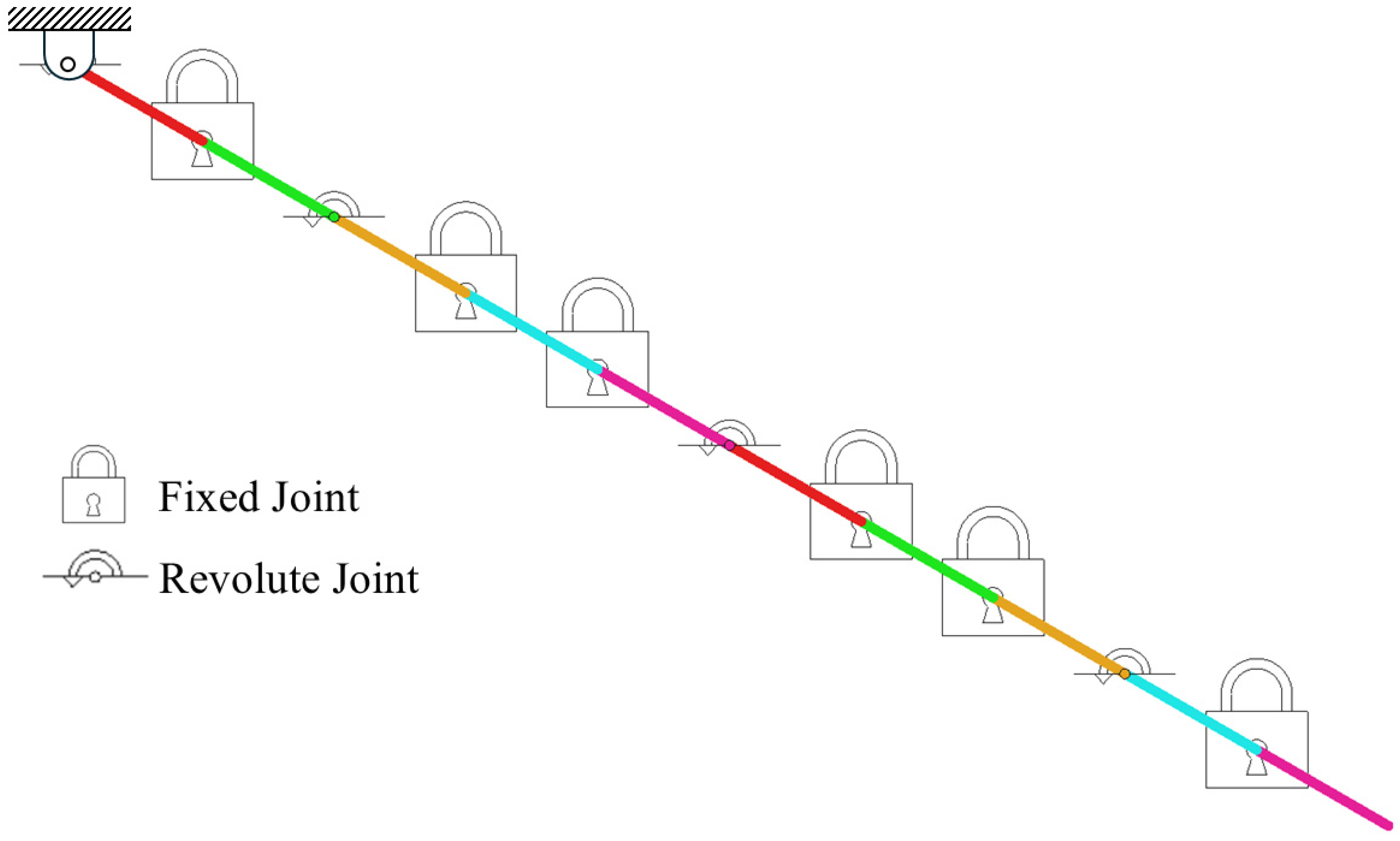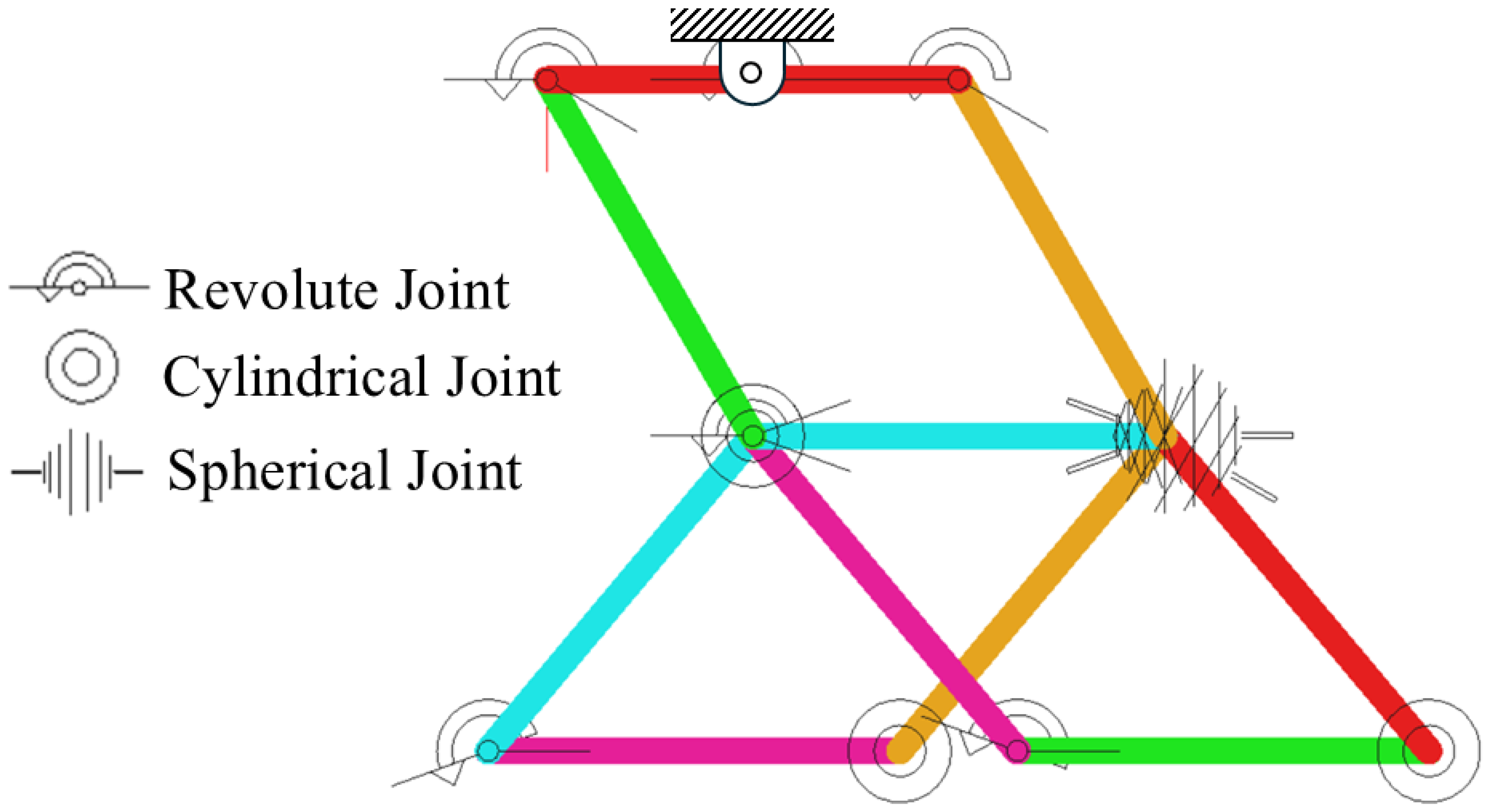Figure 1 and Figure 2 show the open-chain and closed-chain variants of the system, respectively. The two models are identical in terms of masses, inertias, link lengths, and the total number of governing equations, and both are subjected only to gravity loading. The only difference lies in their topological arrangement, open versus closed, which enables isolation and examining the numerical impact of system topology on the computational cost.

The simulations highlight the numerical differences between the two configurations. For the closed-chain model, the solver required 32,319 steps, 33,382 iterations, and 6.11 s of computation time, with an RMS acceleration of 6.51 m/s². For the open-chain model, two simulations were performed to emphasize the role of accelerations in determining the solver effort. In the first case, where the system was initialized at 60° from the vertical, the solver required 34,429 steps, 35,496 iterations, and 4.52 s of computation time, with an RMS acceleration of 10.86 m/s². In the second case, initialized at 30° from the vertical, the solver required only 19,614 steps, 19,707 iterations, and 3.00 s of computation time, with an RMS acceleration of 3.72 m/s².

When normalized by the number of integration steps, the average computational cost per step was 1.89 × 10⁻⁴ s/step for the closed-chain system, 1.31 × 10⁻⁴ s/step for the open-chain system at 60°, and 1.53 × 10⁻⁴ s/step for the open-chain system at 30°. These values confirm that closed-chain systems incur a higher per-step computational burden due to denser Jacobian matrices and more expensive factorizations. At the same time, the total runtime is strongly influenced by the dynamic response: higher accelerations in the open-chain case (60°) led to a greater number of integration steps and longer runtime, while the lower accelerations in the 30° case allowed faster completion despite the same formulation.

This dual effect illustrates a central challenge of simulating constrained mechanisms with classical MBD formulations: the solver is forced to handle both the algebraic stiffness introduced by constraints and the numerical consequences of high accelerations. By contrast, the DBD method does not suffer from these limitations. Since it eliminates algebraic constraints, its numerical stability is governed primarily by the system’s physical natural frequencies rather than by constraint-induced accelerations. Consequently, closed-chain topologies do not introduce additional stiffness into the integration process, and the expected performance advantage of DBD becomes more pronounced in highly constrained or dynamically rich systems.

2.3. DBD Method

In DBD, joints are represented as sets of springs and dampers, which allow for element-wise operations instead of matrix-based calculation, simplifying the overall computation.

The DBD method involves two primary entities: bodies and forces. A body is defined by its mass, inertia, and points associated with it in the body coordinate system (BCS). A force is characterized by the connection points where the spring-damper system operates, along with the spring and damper constants and the free length of the springs. The method utilizes 3-2-1 Euler angles (yaw-pitch-roll sequence) for rotational transformations [27].

A key principle of the DBD method is the replacement of full matrix operations with element-wise calculations. In this approach, two vectors are constructed, each containing the linear indices of points connected by the spring-damper system. This not only enables element-wise operation but also significantly enhances computational efficiency by optimizing memory access patterns. By organizing data in a manner that minimizes cache misses and maximizes memory locality, the DBD method reduces the overhead associated with large-scale matrix computations, leading to more scalable and efficient simulations.

The first step in the DBD method is to calculate the coordinates of the body points in the world coordinate system (WCS). The second step involves computing the equivalent spring and damper constants and updating the positions of the points that can move relative to their respective bodies. This step is only necessary in special cases, such as when torsion springs are involved [18].

Once the points are defined in the WCS, the distance between each pair of points connected by the spring-damper system is calculated. Velocities between these points are computed using the backward Euler method. This process is applied to all forces in the system using element-wise products, as all forces and joints are modeled by springs and dampers.

The next step involves transforming the forces from the WCS to the BCS. All forces and torques acting on each body in the BCS are then aggregated. A vector Q is created, containing 6n elements that represent the total forces and torques in the BCS of each body:

$$\begin{array}{l}{Q}_{6i-11}=\sum {\mathit{F}\mathit{o}\mathit{r}\mathit{c}\mathit{e}\mathit{B}\mathit{C}\mathit{x}}^i+{Fx}^i\\ Q_{6i-10}=\sum {\mathit{F}\mathit{o}\mathit{r}\mathit{c}\mathit{e}\mathit{B}\mathit{C}\mathit{y}}^i+{Fy}^i\\ \begin{array}{l}{Q}_{6i-9}=\sum {\mathit{F}\mathit{o}\mathit{r}\mathit{c}\mathit{e}\mathit{B}\mathit{C}\mathit{z}}^i+{Fz}^i\\ Q_{6i-8}=\sum {\mathit{T}\mathit{o}\mathit{r}\mathit{q}\mathit{u}\mathit{e}\mathit{B}\mathit{C}\mathit{x}}^i+{Tx}^i-\left(I_{yy}^i-I_{zz}^i\right){\omega }_y^i{\omega }_z^i\\ \begin{array}{c}{Q}_{6i-7}=\sum {\mathit{T}\mathit{o}\mathit{r}\mathit{q}\mathit{u}\mathit{e}\mathit{B}\mathit{C}\mathit{y}}^i+{Ty}^i-\left(I_{zz}^i-I_{xx}^i\right){\omega }_z^i{\omega }_x^i\\ Q_{6i-6}=\sum {\mathit{T}\mathit{o}\mathit{r}\mathit{q}\mathit{u}\mathit{e}\mathit{B}\mathit{C}\mathit{z}}^i+{Tz}^i-\left(I_{xx}^i-I_{yy}^i\right){\omega }_x^i{\omega }_y^i\end{array}\end{array}\end{array},$$

(4)

where ForceBCjⁱ is the force vector acting on body i in direction j, and TorqueBCjⁱ is the torque vector acting on body i in the j direction in the BCS. Fjⁱ is an external force acting on the center of mass (CG) of body i in the j direction in the BCS and Tjⁱ is an external torque action on body i around the j direction in the BCS. ${\omega }_j^i$ is the angular velocity of body i in the j direction in the BCS. $I_j^i$ is the inertia moment of body i around the j direction. The index i = 1 corresponds to the world body, for which forces are not calculated. The vector Q is associated with all bodies except the world body. The above formulation assumes that the body coordinate system coincides with the principal axes of inertia, such that the cross products of inertia vanish (I_xy = I_xz = I_yz = 0).

Note that in order to calculate the total torque on each body, it is first necessary to determine the body’s velocities in the BCS. The body’s velocities in the WCS are known from the initial conditions or from the previous time step. These linear velocities are transformed from WCS to BCS.

The acceleration of each body in the BCS is calculated using element-wise division:

$${\ddot{\mathit{q}}}_{BC}=\mathit{Q}\oslash \mathit{m},$$

(5)

where m is a vector of masses and inertias for n bodies written as:

$$m={\left[\begin{array}{ccc}{m}^1& m^1& \begin{array}{ccc}{m}^1& I_{xx}^1& \begin{array}{ccc}{I}_{yy}^1& I_{zz}^1& \begin{array}{ccc}\dots & m^n& \begin{array}{ccc}{m}^n& m^n& \begin{array}{ccc}{I}_{xx}^n& I_{yy}^n& I_{zz}^n\end{array}\end{array}\end{array}\end{array}\end{array}\end{array}\right]}^T.$$

(6)

Following the calculation of accelerations in the BCS, the velocities are updated using the Adams-Bashforth method (1st order) for velocity prediction and corrected using the Backward Differentiation Formula (BDF) 1st order. The Adams-Moulton method (2nd order) is then used for velocity calculation. This combination of methods is referred to as ABAM.

The velocities are transformed back to the WCS. The positions are updated using a semi-implicit 1st-order Euler method, based on the velocities obtained from the ABAM method.

Once the integration stage is complete, the system undergoes a convergence process using the Newton–Raphson method, as:

$$\left[\begin{array}{c}{\dot{\mathit{q}}}^{i+1}\\ {\mathit{q}}^{i+1}\end{array}\right]=\left[\begin{array}{c}{\dot{\mathit{q}}}^i\\ {\mathit{q}}^i\end{array}\right]-{\mathit{J}}^{-1}\mathit{G}.$$

(7)

The Jacobian matrix for this method is:

$$\mathit{J}=\left[\begin{array}{cc}{\mathit{D}}_{6n\times 6n}& {\mathit{O}}_{6n\times 6n}\\ {\mathit{I}}_{6n\times 6n}& -{\mathit{I}}_{6n\times 6n}/h\end{array}\right],$$

(8)

where D is a diagonal matrix of m, and h is the time step size. The Jacobian matrix has two diagonals (major and minor). This matrix is smaller than the Jacobian matrix used in traditional MBD, as it does not involve constraint elements. Additionally, the matrix is constant, allowing it and its inverse to be precomputed before the iterative process. The inverse matrix’s structure also involves only two diagonals (major and minor), enabling efficient convergence through element-wise operations. The form of the inverse matrix is written as:

$${\mathit{J}}^{-1}=\left[\begin{array}{cc}{\mathit{D}}_{6\mathit{n}\times 6\mathit{n}}^{-1}& {\mathit{O}}_{6\mathit{n}\times 6\mathit{n}}\\ \mathit{h}{\mathit{D}}_{6\mathit{n}\times 6\mathit{n}}^{-1}& -\mathit{h}{\mathit{I}}_{6\mathit{n}\times 6\mathit{n}}\end{array}\right].$$

(9)

Vector G (from Equation (7)) contains 12n elements due to the order reduction. Because positions in the BCS are irrelevant, the velocities in the WCS are calculated first and then transformed into the BCS. G is written as:

$$\mathit{G}=\left[\begin{array}{c}\mathit{m}{\displaystyle \frac{{\dot{\mathit{q}}}_{BC}^{i+1}-{\dot{\mathit{q}}}_{BC}^i}{h}}-\mathit{Q}\\ {\dot{\mathit{q}}}_{BC}^{i+1}-{\left({\displaystyle \frac{{\mathit{q}}_{WC}^{i+1}-{\mathit{q}}_{WC}^i}{h}}\right)}_{WCS\to BCS}\end{array}\right].$$

(10)

It is important to note that the use of Euler angles with a yaw-pitch-roll sequence can lead to gimbal lock, particularly at a pitch of ±π/2 rad. To avoid this, the current implementation rotates the world frame when the pitch angle of a body gets close to ±π/2. In future versions, dual rotation sequences will be evaluated in parallel, and the sequence that is furthest from gimbal lock will be selected for use.

2.3.1. DBD Numerical Scheme

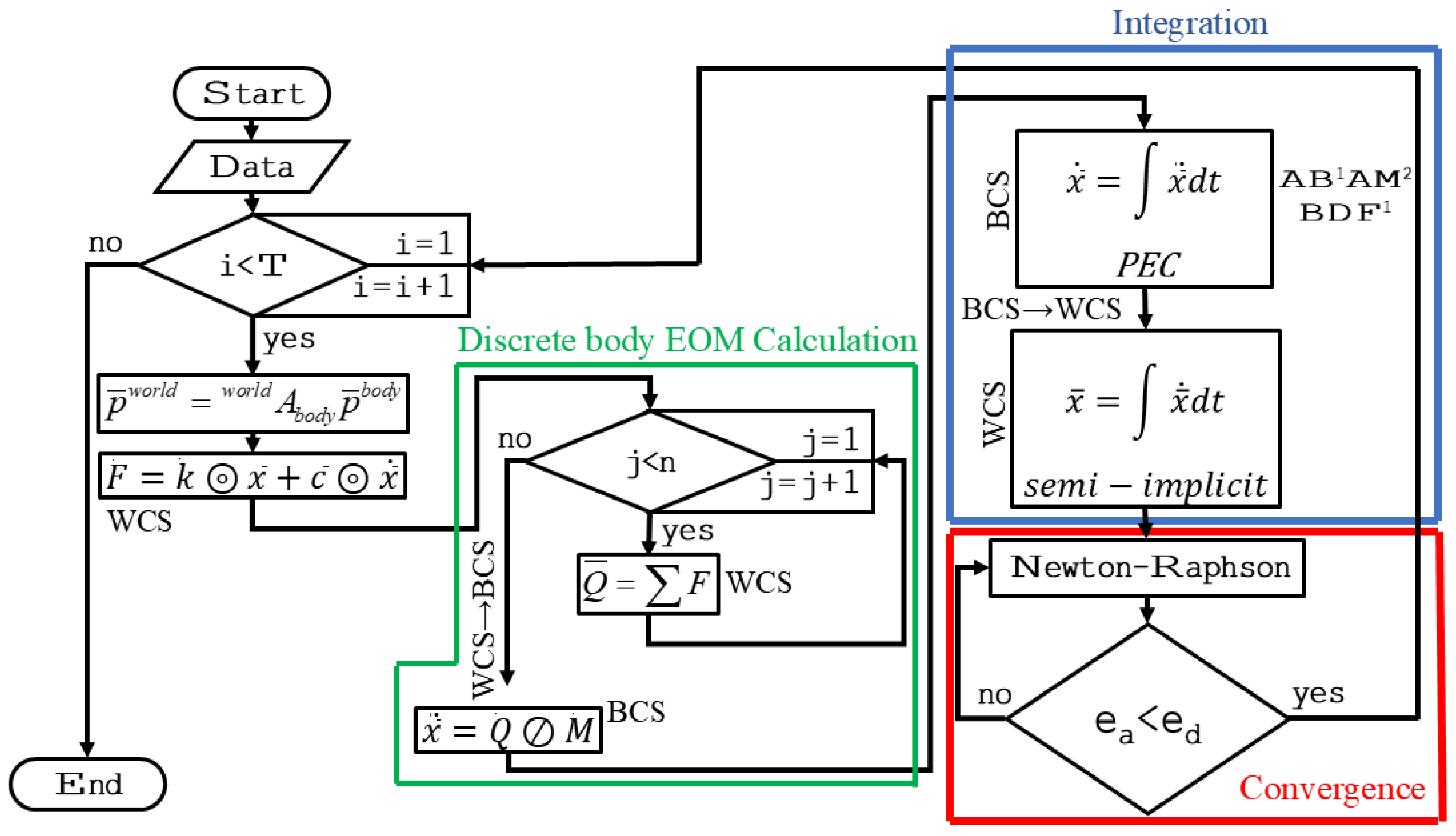
To conclude the DBD method, the numerical scheme comprises the following sequential steps [18], as illustrated in the flowchart in Figure 3:

• Calculation of Point Positions: Utilizing the transformation matrix from BCS to WCS, the positions of points are computed.
• Force Computation: Forces are determined based on point displacements and velocities.
• Summation of Forces and Moments: Forces and moments acting on each body are summed independently within the body coordinates.
• Acceleration Calculation: The accelerations of each body are computed by elementwise division of the force vector with the mass and inertia vector.
• First Integration (Predict-Evaluate-Correct—PEC): Velocity calculation is carried out through the predict-evaluate-correct method, employing Adams–Bashforth (1st order), backward differentiation formula (BDF) (1st order), and Adams–Moulton (2nd order) methods.
• Second Integration (Semi-Implicit): Following the transformation from BCS to WCS, a second, semi-implicit integration (1st order) is executed.
• Convergence using the Newton–Raphson method: Employing the 1st-order BDF, convergence is achieved through Newton–Raphson. The inverse of the Jacobian matrix, a two-diagonal constant matrix, facilitates convergence through the elementwise product.

2.3.2. DBD Advantages

The DBD methodology offers several advantages [18]:

• Enables the modeling of compliance in the joints, such as bushings.
• Alleviates the introduction of additional constraint equations that lead to the formulation of DAE.
• Facilitates the separate resolution of each body, making it conducive to parallel computation.
• Eliminates the need for matrix decomposition and uses element-wise products instead.
• Mitigates issues associated with ill-conditioned systems, allowing the combination of lightweight and heavy bodies or the utilization of very small time steps for the examination of specific dynamical phenomena.
• Utilizes a constant Jacobian matrix for the Newton–Raphson convergence,
• Possesses a computational complexity of O(n).

2.4. Joint Representation

As previously mentioned, a set of translational springs and dampers is utilized to represent the constraints. The dynamic performance closely approximates that of an ideal joint when these springs are sufficiently stiff. However, a small time step is required to ensure precise modeling. In instances where there is no available data on the joint damping constant, it is set to yield a damping coefficient of one. Determination of the system frequencies of spring extension becomes crucial for calculating the damping constant, c, achieved through c = 2k/w_n, where k is the spring constant used for joint representation and w_n is the natural frequency of this spring.

The above damping rule follows directly from the classical second-order damping-ratio form $c=2\zeta \sqrt{k m_{\mathrm{e}\mathrm{f}\mathrm{f}}}$ together with ${\omega }_n=\sqrt{k/m_{\mathrm{e}\mathrm{f}\mathrm{f}}}$, where $m_{\mathrm{e}\mathrm{f}\mathrm{f}}$ denotes an effective (modal) mass associated with the TSDA extension along its line of action. Since ${\omega }_n$ is identified from the TSDA-extension response, the corresponding effective mass, and its configuration dependence, is implicitly embedded in the identified ${\omega }_n$. When damping data are available (e.g., from experiments or manufacturer specifications), the corresponding $\zeta$ (or equivalently $c$) should be used directly; $\zeta =1$ is only a representative default in the absence of such information.

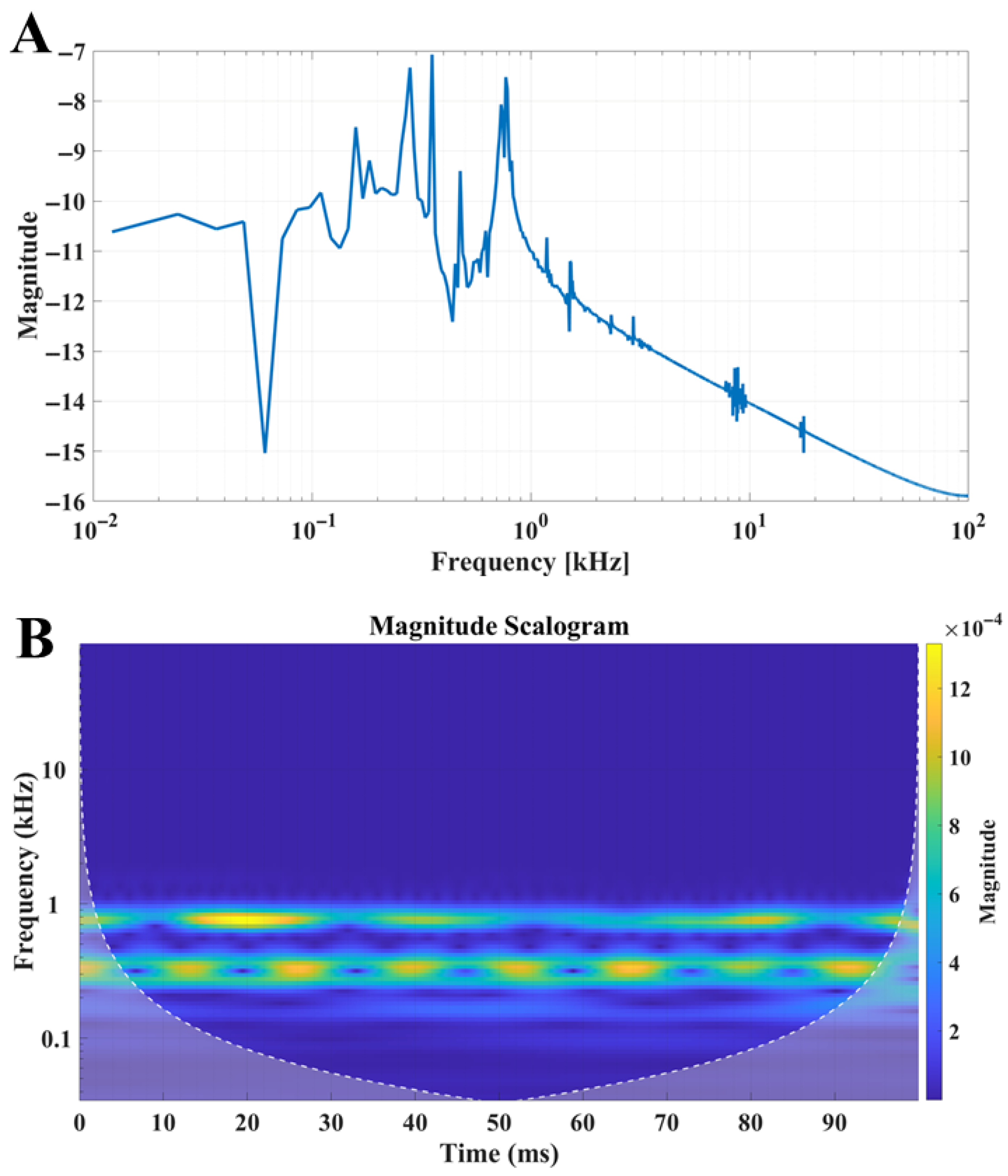
Frequency analysis is typically performed using the Fast Fourier Transform (FFT). However, achieving clear frequency distinction is challenging. Therefore, it is advisable to employ wavelet analysis for enhanced clarity in frequency separation. Figure 4 illustrates both representations for the spring extension signal of the 3RUU mechanism: Figure 4A shows the FFT magnitude spectrum in the frequency domain, where the horizontal axis is frequency (kHz) and the vertical axis is the spectrum magnitude. Figure 4B shows the wavelet time–frequency scalogram, where the horizontal axis is time (ms), the vertical axis is frequency (kHz), and the color indicates magnitude. To excite the system, the free lengths of selected springs were perturbed by 1 mm. The dominant natural frequency is identified as the frequency associated with the maximum magnitude (here ≈ 752 Hz), and this value is used as the representative frequency for the time-step selection criterion.

In the proposed DBD formulation, joints are realized via spring/TSDA elements rather than ideal kinematic constraints; therefore, the model does not exhibit classical over-constraint in the DAE sense (i.e., redundant constraint equations). Instead, the main numerical challenge is ODE stiffness: when a joint is modeled as very stiff, the resulting system contains high dominant natural frequencies, which require a sufficiently small integration step for stable and accurate explicit time integration. In practice, joint stiffness in DBD is selected primarily to reflect the intended physical compliance of the connection. Typical stiffness levels reported for automotive rubber bushings span from a few tens to a few hundreds of N/mm [28], while substantially higher stiffness levels can also occur for stiffer bushing concepts, reaching and exceeding an order of 1000 N/mm (e.g., reported conventional-bushing stiffness above 1000 N/mm and measured stiffness in the range of about 1312–1562 N/mm in a magnetorheological-elastomer bushing study [29]).

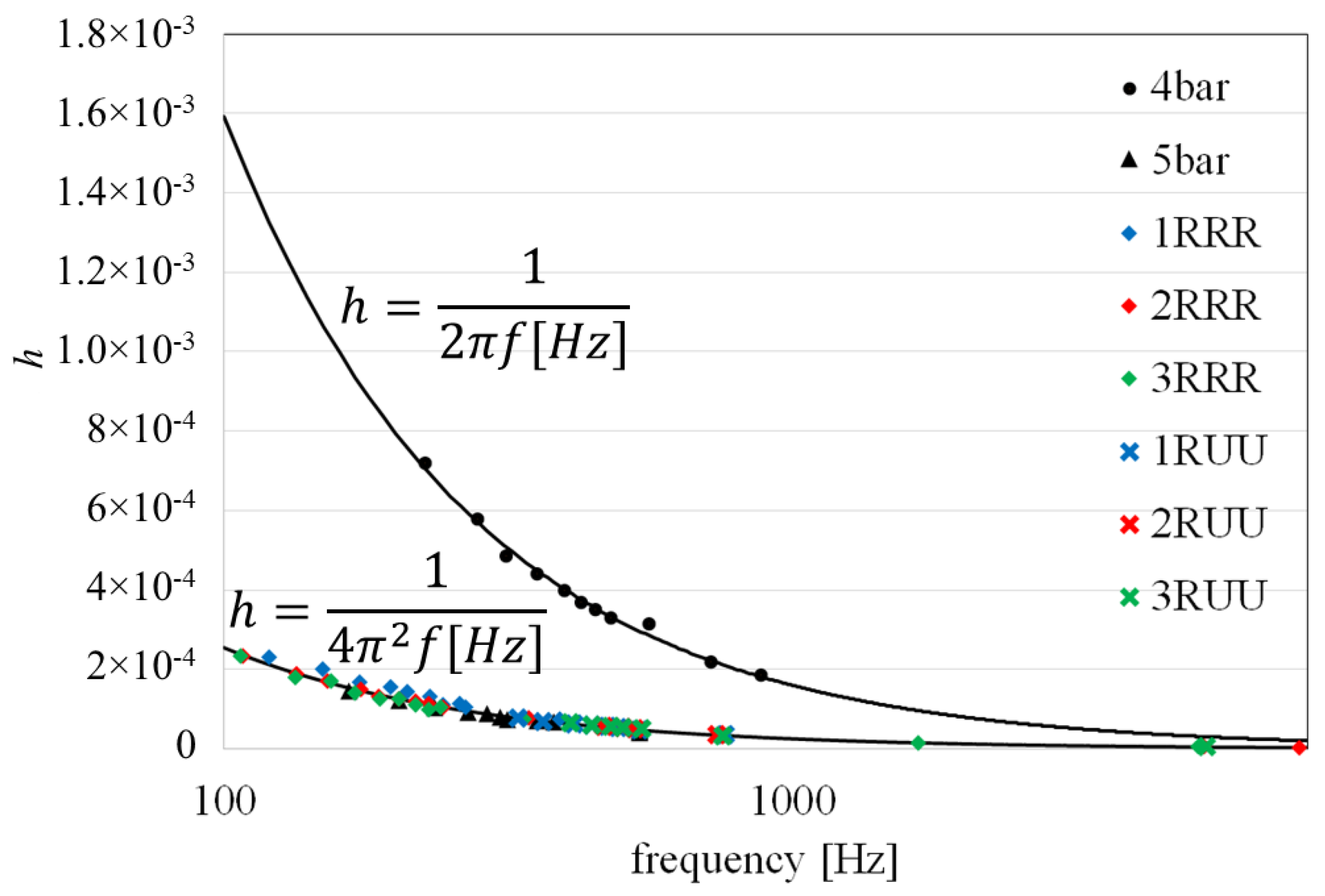
To balance ideal-constraint approximation and numerical stability, DBD therefore couples stiffness selection with a time-step selection criterion based on the dominant natural frequency of the resulting compliant model. This criterion provides a practical safeguard against instability while allowing the user to tune compliance realistically.

Finally, because explicit integration cost scales with the highest relevant frequency, near-ideal (very stiff) joints can make DBD computationally expensive, since stable integration may require very small time steps. In such regimes, classical constraint-based MBD solvers with variable-step stiff integration can become more efficient. Nevertheless, DBD can still simulate these cases by further reducing the time step, at the cost of substantially longer runtimes, while retaining the ability to reach high accuracy.

2.4.1. Spherical and Revolute Joint

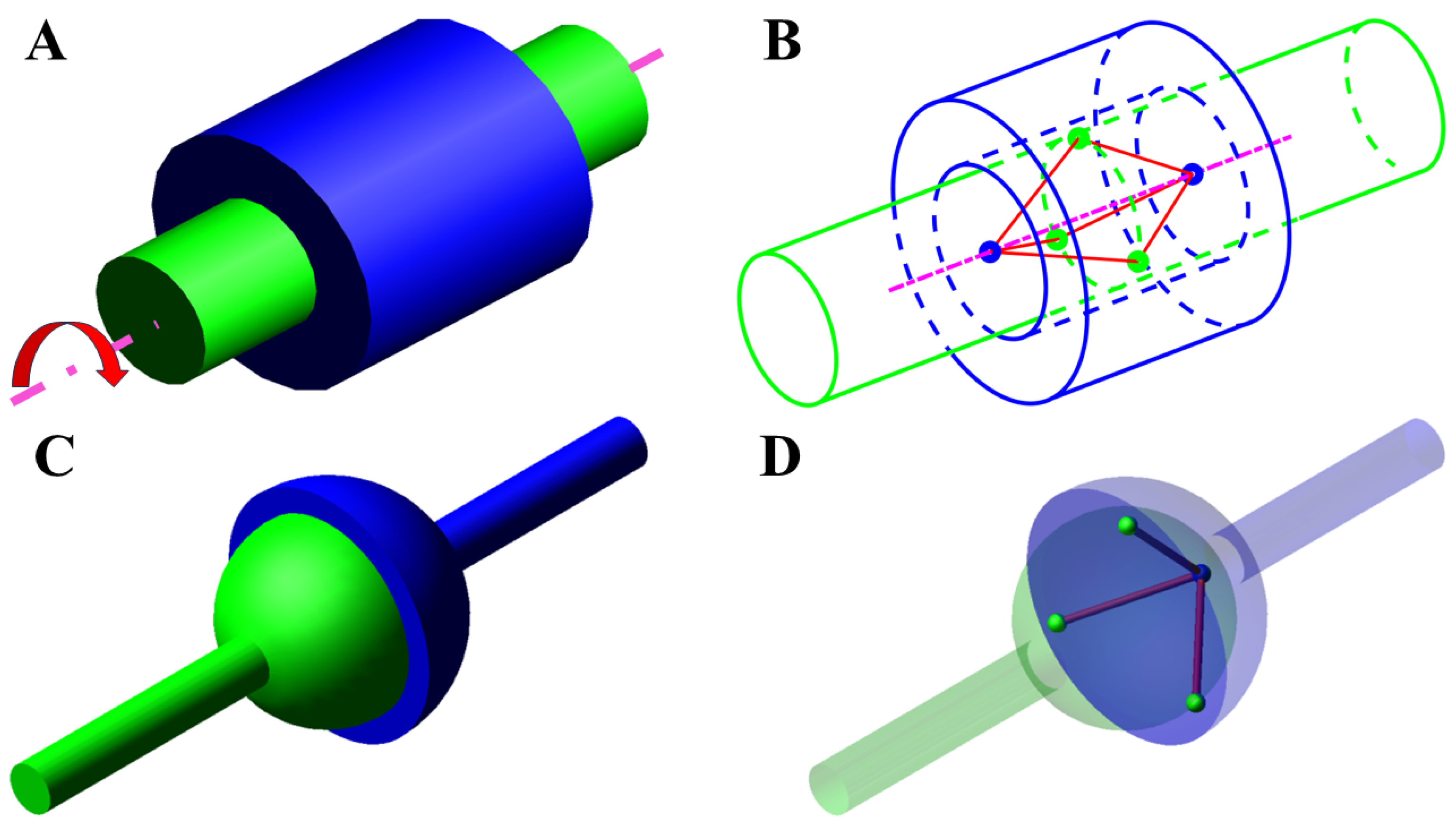
The revolute joint, depicted in Figure 5, is represented through six TSDA—three on each side. The two blue points pertain to the blue outer cylinder, while the three green points are associated with the green inner rod. The six red lines, connecting the corresponding blue and green points, symbolize the TSDAs. This configuration enables unrestricted rotation about the magenta axis, representing the rotational axis, while constraining movements in other directions. Such a definition of the revolute joint is instrumental in accurately modeling compliant revolute joints, including those exhibiting bushings. If data on a particular bushing is unavailable, its properties can be determined through experimental analysis of its dynamic behavior. For instance, in a study investigating rubber bushings situated at the radiator and intercooler of an SUV diesel vehicle, the damping coefficient was found to be 0.007 (5.9 N·s/m) and 0.009 (5.5 N·s/m), respectively [28].

The spherical joint is the same as the revolute joint but uses just three TSDAs. This means three TSDAs from three points associated with one body are connected to a single point associated with the other body.

2.4.2. Universal Joint

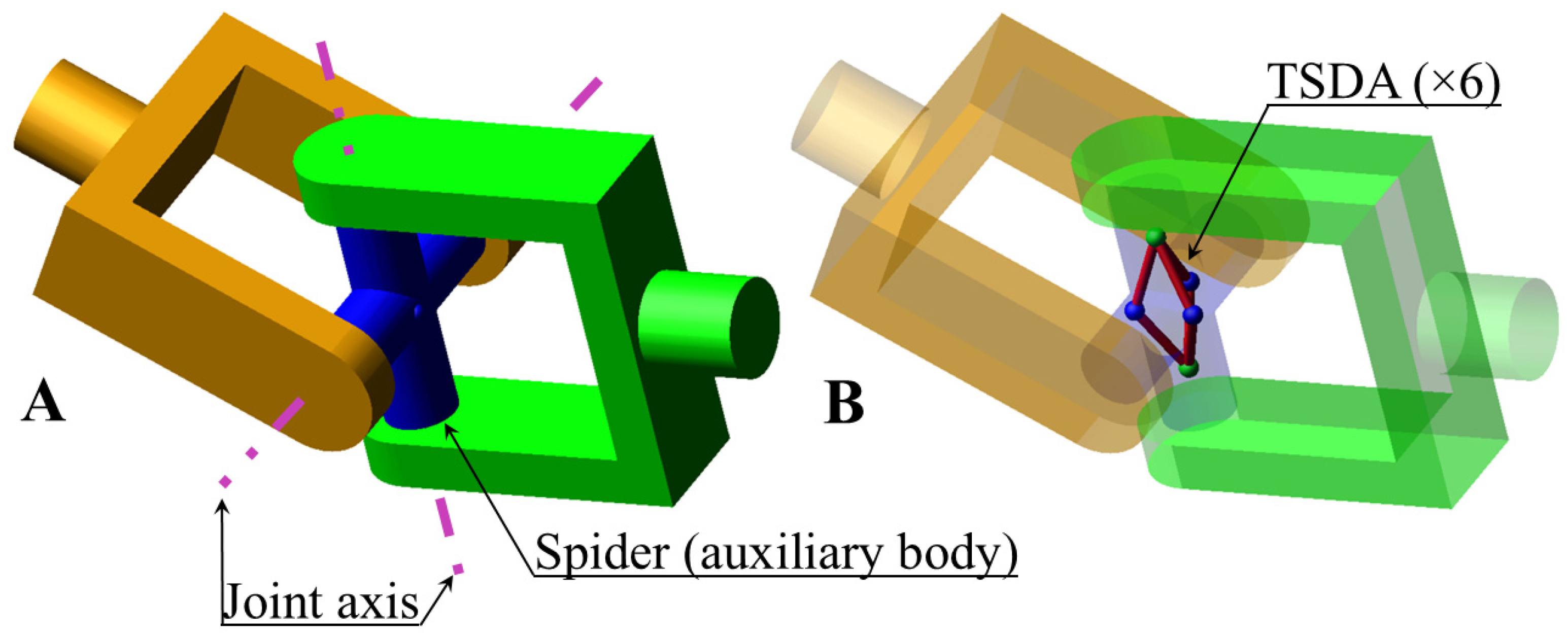
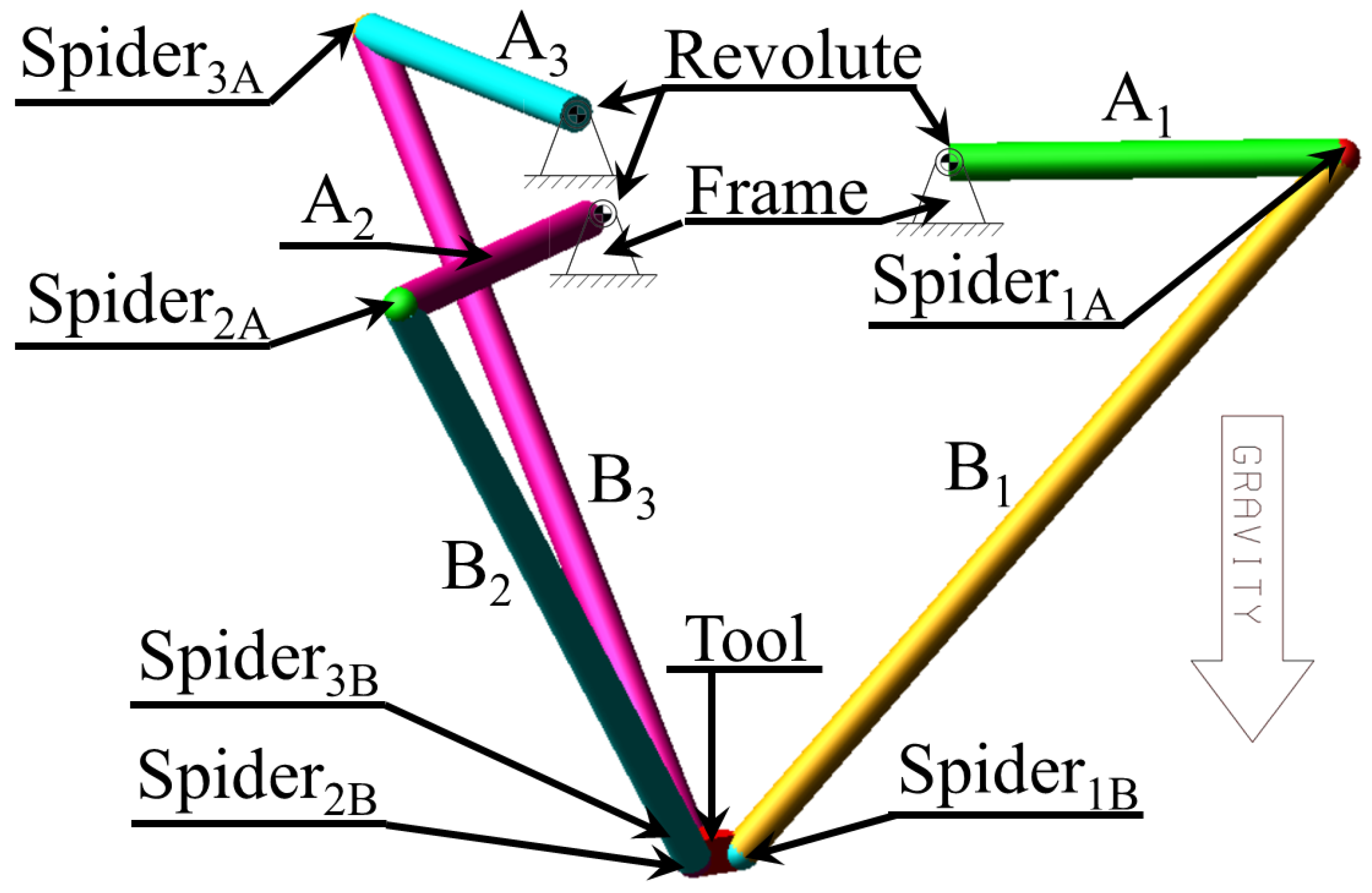
The universal joint, depicted in Figure 6, is a frequently encountered element in spatial and closed-chain systems. For clarity, Figure 6B shows only one representative spider-to-link revolute sub-connection; the remaining connections are identical by symmetry. Comprising two revolute joints, its representation within the DBD modeling approach necessitates the introduction of a central component known as the “spider body.” This central element serves to connect the two rods effectively. Furthermore, two revolute joints must be defined following the methodology outlined in Section 2.4.1. Accordingly, a total of 12 springs and dampers are indispensable for an accurate modeling of the universal joint. Due to the complex structure of the TSDAs, they are omitted from Figure 6 for clarity.

2.4.3. Cylindrical and Translational Joint

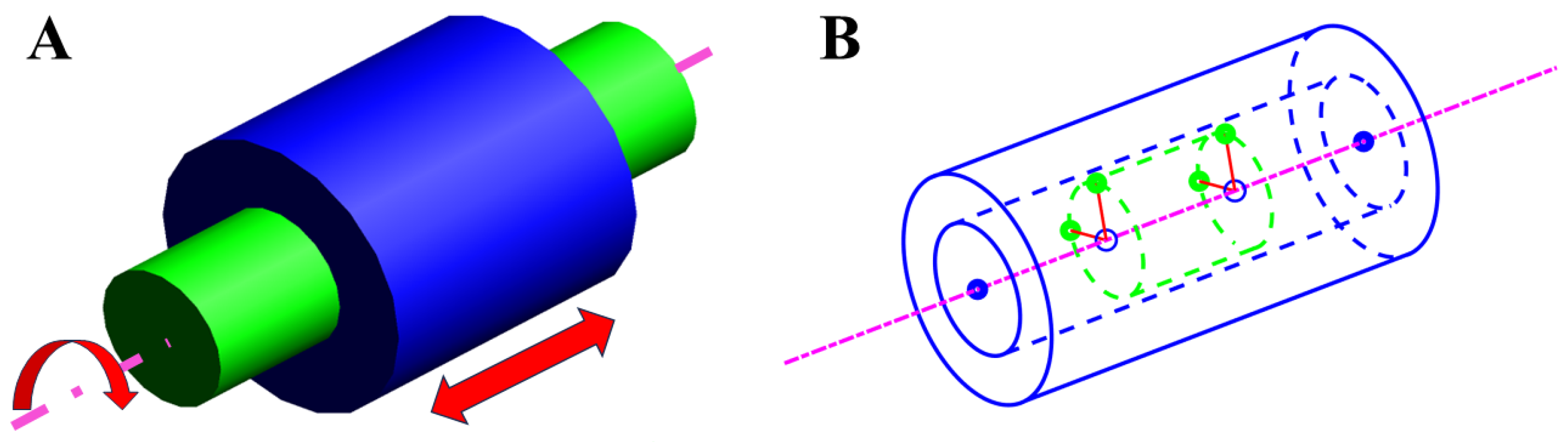
The cylindrical joint, allowing it to translate and to rotate around the same axis, is depicted in Figure 7. It consists of two bodies: the cylinder (the blue body) and the piston (the green body). To represent this joint using only TSDAs (red lines), two points (blue points) are defined on the cylinder body, positioned at both ends. These points define the vector along which the piston body is constrained to move (magenta dash-dotted line). Additionally, four points (green points) are defined on the piston body, illustrated in Figure 7.

The four points on the piston body are projected onto the vector defined by the cylinder. This projection determines the corresponding points on the cylinder’s vector. Each point on the piston body is then connected to its corresponding point on the cylinder vector using TSDAs.

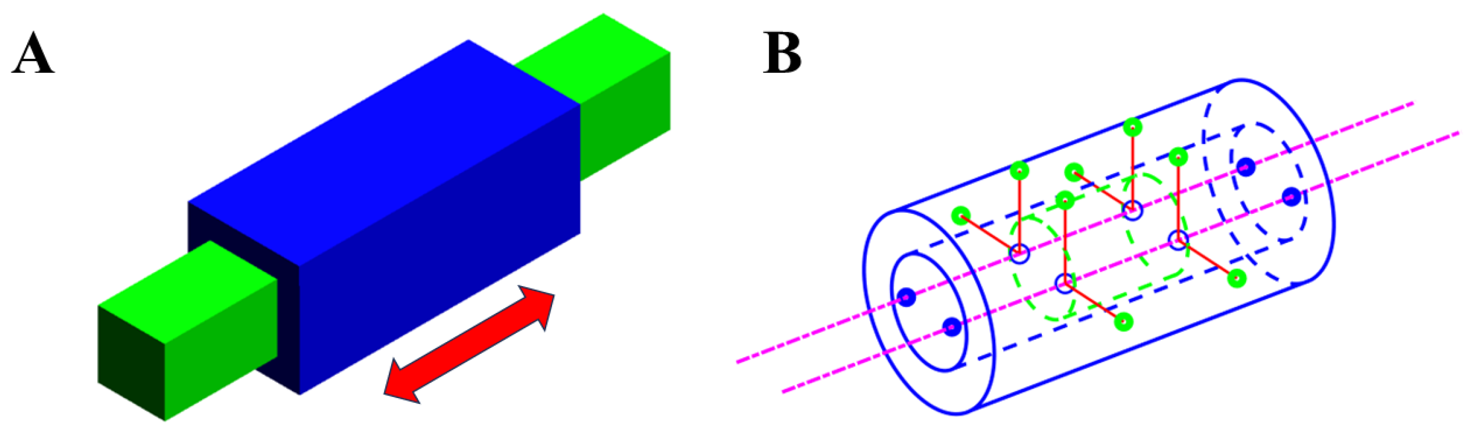
For a translational joint (Figure 8) that restricts around the translational axis, an additional vector (represented by the magenta dash-dotted line) is defined on the cylindrical body. Eight points are defined on the piston body, with four points located at each end of the piston (these points may extend beyond the geometric boundaries of the body). At each end, two points are connected to one of the translational axes, with the vectors linking these points to the translational axis being orthogonal to each other. All four points at each end are projected onto the adapted translational axis. This representation aligns with the numeric scheme of the DBD method, enabling the calculation of TSDA forces through element-wise products, as is done for all forces in the model.

3. Comparison Method

One of the advantages of the DBD method is its computational complexity, which is O(n) due to the independent resolution of each body. Conversely, a disadvantage of the DBD method lies in the requirement for a small time-step size due to the stiffness of the springs representing joints within the model. Thus, the effectiveness of the DBD method is most pronounced when dealing with models that consist of many bodies and constraints and when the joints are not excessively stiff. Stiff joints introduce high frequencies, necessitating a smaller time step size. Hence, an investigation into solver performance can delineate various scenarios based on the number of bodies and the natural frequencies of a dynamic system, tailoring them to suit each solver type (MBD or DBD). Additionally, the mechanism topology influences dynamic behavior and may affect the solver’s performance.

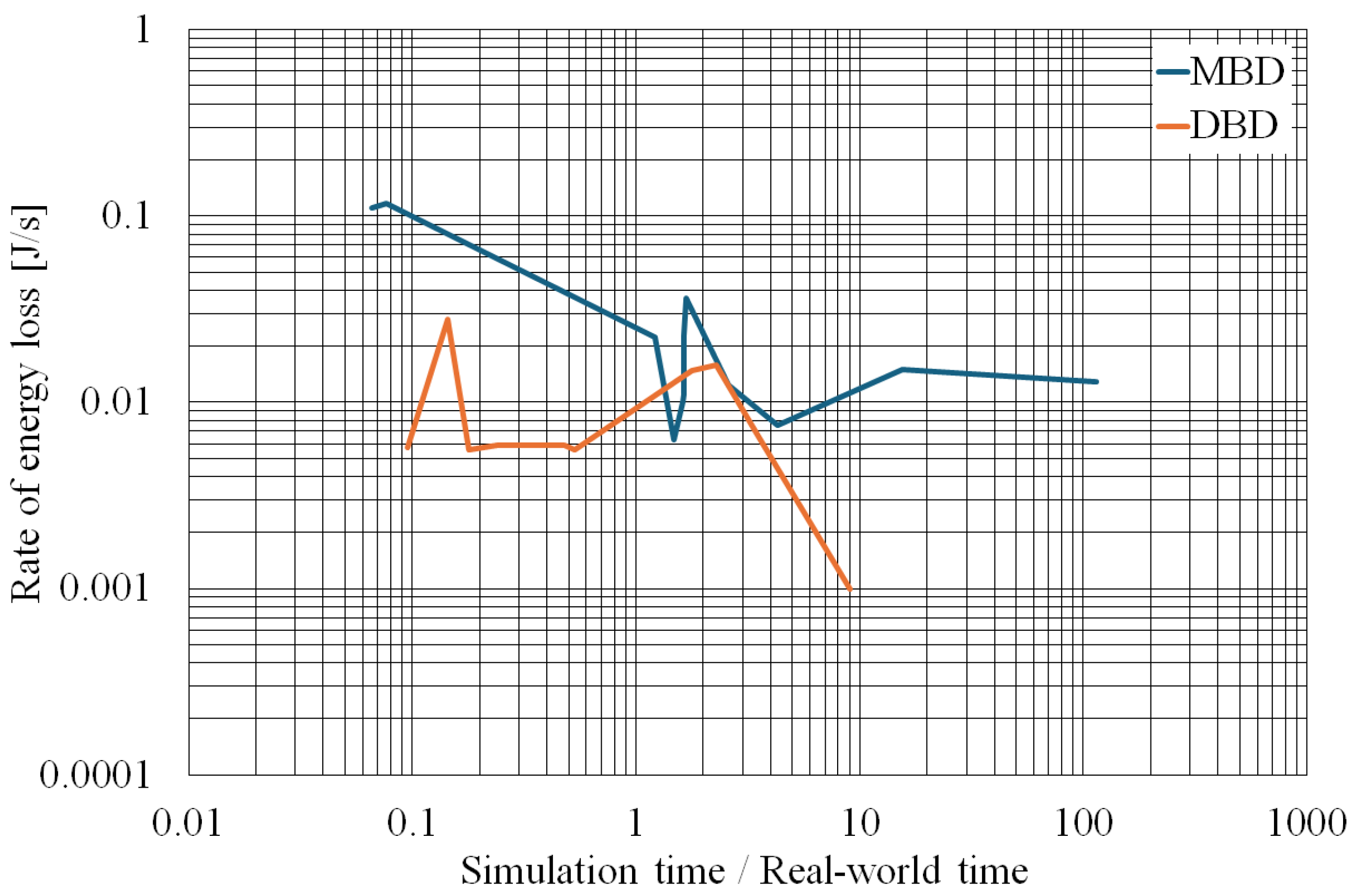
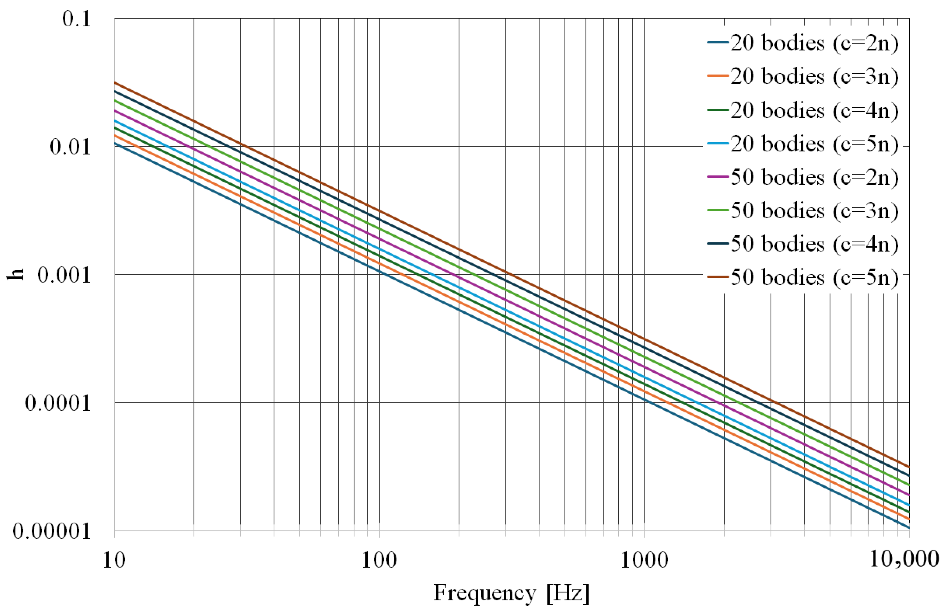
Solver performance can be estimated by accuracy and solution speed. In an energy-conservative system, the magnitude of energy change indicates the solution’s accuracy. Furthermore, as the stiffness of the springs representing the joints increases, the dynamic system behavior of the DBD model becomes more similar to that of the MBD model, where the joints are represented by constraints. Therefore, this comparison can serve as an indicator of the solution’s validity. The solution speed is affected by the time step size, h, and the actual duration to perform a single time step, τ. While h depends on the numerical scheme, system frequencies, and the number of bodies and constraints, τ also depends on the solver’s development environment.

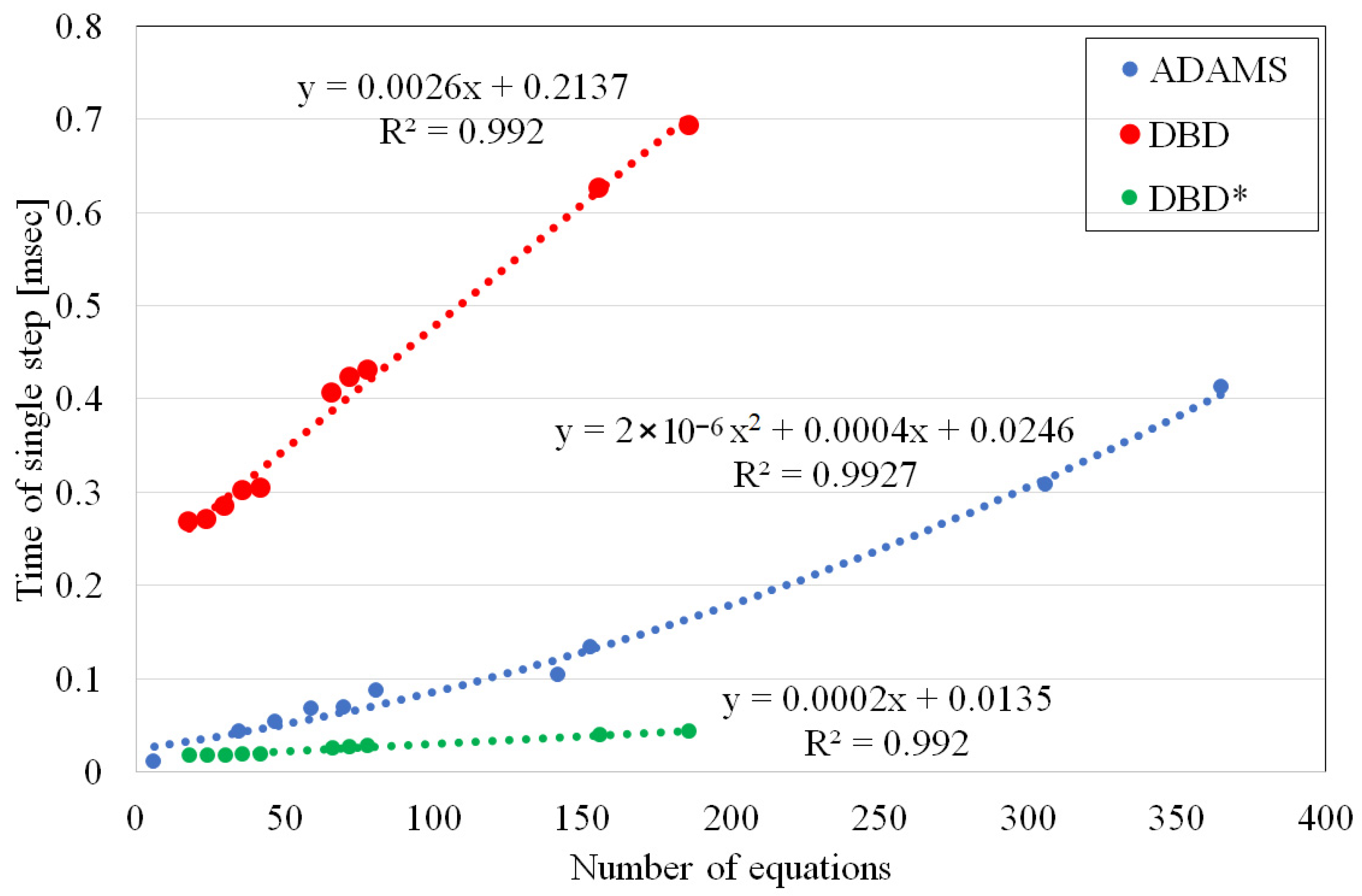
To compare these aspects, we investigated the influence of the number of bodies and constraints on the duration of a single time step, τ. This comparison is conducted on the systems detailed in Section 3.2, using different configurations to achieve ten different systems with varying numbers of bodies and constraints. To normalize the results and eliminate the influence of the programming language and program development efficiency, we divided the duration of a single time step by an adjusting factor F, detailed in Section 3.1.

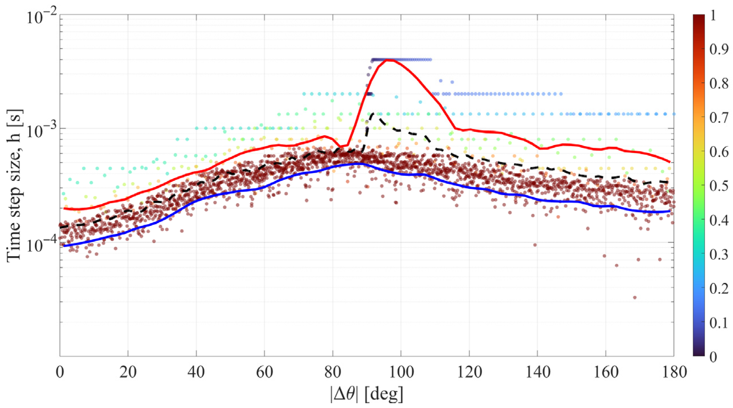
Another aspect under investigation is the influence of frequency on the time step size, h, in the DBD solver. In this analysis, we aim to determine the largest possible time step size without the solution becoming divergent. Subsequently, we explored the significance of two factors on the accuracy of the DBD method: the time step size and the stiffness of the joints. To assess the accuracy, we solved the model dynamics using the DBD method with very stiff joints and a very small step size.

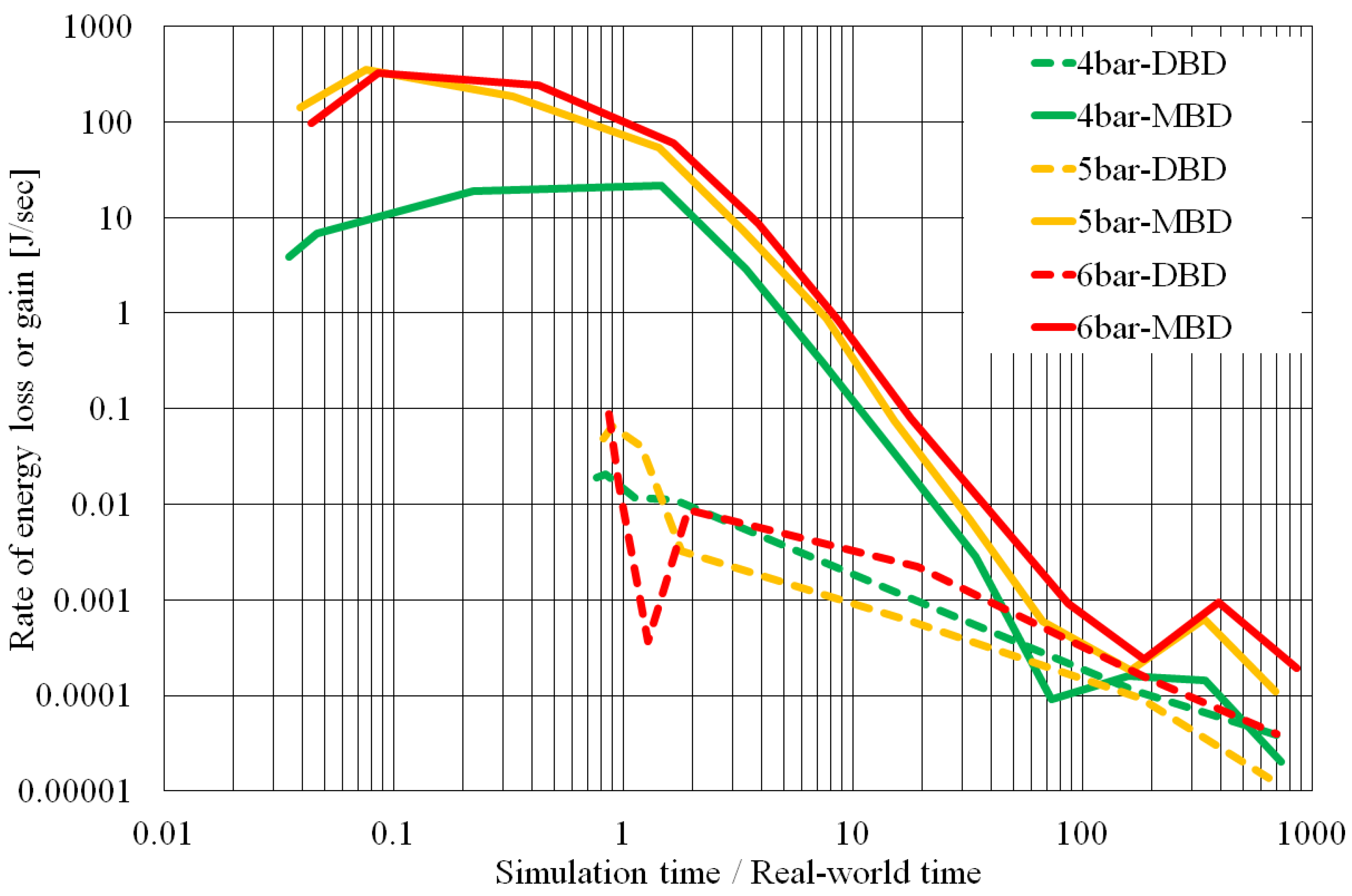
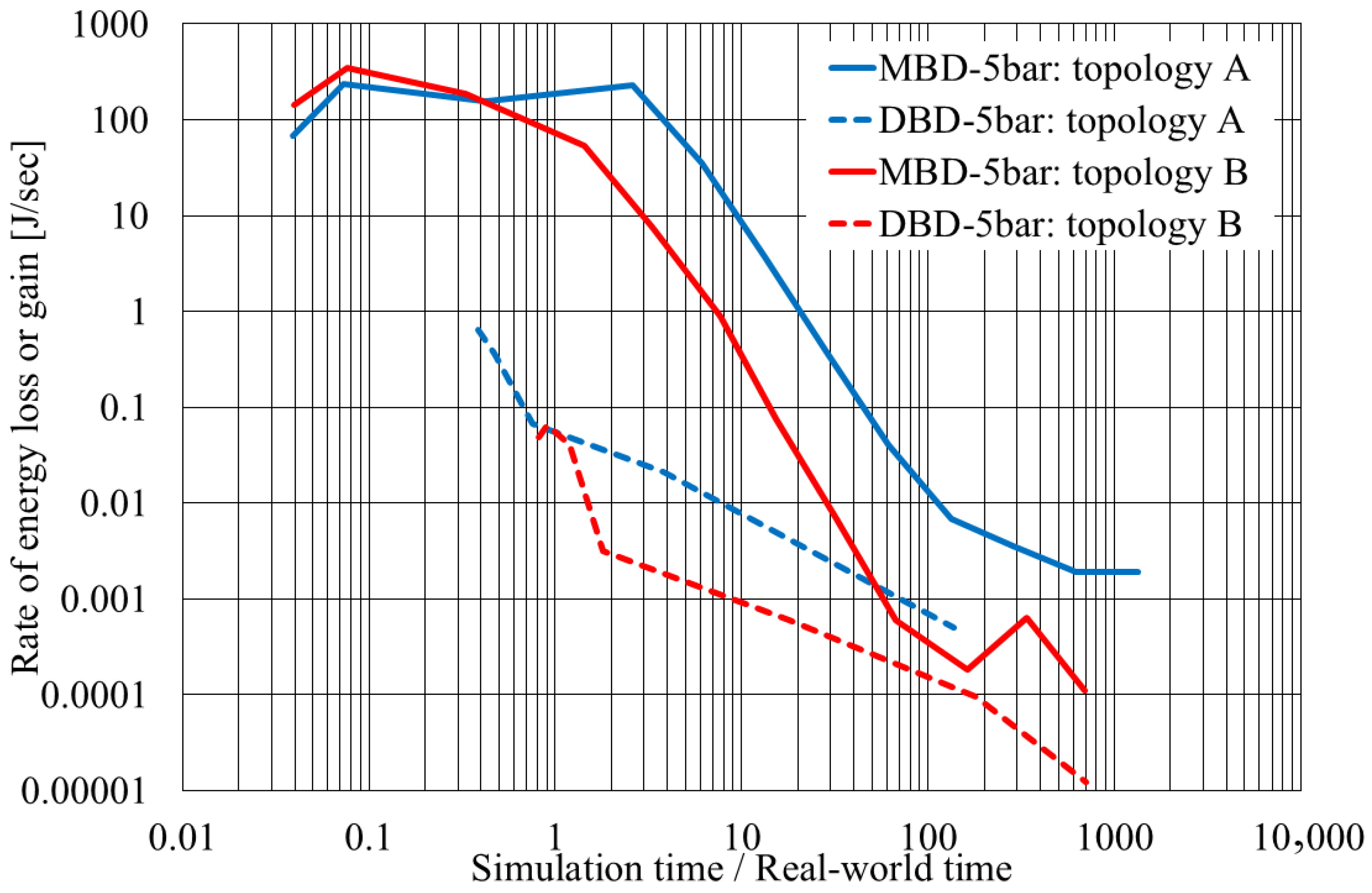
Integrating all these investigations, we compared the solver’s performance in terms of accuracy and solution speed. This comparison was conducted on conservation systems (without damping). Accuracy is defined as the rate of energy change, assuming that energy remains constant. Solution speed is defined as the simulation time to real-world time ratio (SRT). An SRT of one represents real-time (RT). An SRT greater than one indicates slower than RT, while an SRT less than one indicates faster-than-real-time (FTRT). This investigation includes the impact of the number of bodies and the topology of the mechanism.

3.1. Computing Environment

All simulations were performed on an Asus VivoBook laptop equipped with an 11th Gen Intel^® Core™ i7-1165G7 processor (4 cores, 8 threads, 2.80 GHz) and 16 GB RAM, and an SSD, running Windows 10 (Version 22H2). Numerical simulations were carried out using MATLAB R2021b and MSC Adams/View 2021.1. No parallel computing capabilities were employed.

All ADAMS simulations were performed using the GSTIFF SI2 integrator with adaptive step-size control and adaptive variable integration order. We performed a tolerance sweep starting from an error tolerance of 0.1 and progressively tightening it. The sweep was stopped when either (i) further tightening of the tolerance produced no observable change in the solution within the reported metrics or (ii) the solver failed to complete the simulation. Unless stated otherwise, all other ADAMS settings were kept unchanged across the sweep.

3.2. DBD and ADAMS/View Computing Time Adjustment

The DBD method was compared to the multibody dynamic method using ADAMS/View of MSC (version 2021.1) as the platform for the multibody dynamic simulations. ADAMS/View is implemented in a high-level, general-purpose programming language, making it efficient commercial software. For the MBD simulations, we employed the GSTIFF SI2 integrator in MSC ADAMS. This solver implements a variable-step, variable-order backward differentiation formula (BDF) scheme, which is widely recognized as the standard choice for stiff differential-algebraic equations (DAEs) [30]. The SI2 option (Stabilized Index-2) provides enhanced treatment of index-2 constraints, reducing numerical drift and ensuring more accurate velocity and acceleration histories, particularly in systems with smooth or high-frequency motions [31].

Numerically, GSTIFF SI2 is well suited for problems with stiff couplings and tightly constrained mechanisms. The stabilized index-2 formulation allows for larger effective time steps or higher error tolerances while maintaining solution accuracy, which is crucial when comparing with the DBD method, where time-step size and numerical stability are key factors.

Moreover, this selection follows both the explicit recommendations of the ADAMS/Solver User’s Guide [31] and the established practice in multibody dynamics research and industry applications, where GSTIFF SI2 is routinely applied to systems involving contacts, stiff joints, and high-frequency dynamics [32]. Choosing a non-stiff or stabilized solver could either fail to converge or require extensive parameter tuning, introducing a bias in the comparison. Therefore, GSTIFF SI2 provides both an industry-relevant and numerically fair baseline for evaluating the performance of the proposed DBD method.

At the same time, DBD is coded in MATLAB R2021b and is still undergoing development, so it is reasonable to expect significant performance differences. As a result, the objective was to identify a study-specific factor (F) that captures the dominant execution environment and implementation overhead of the current MATLAB prototype relative to ADAMS.

We expect reduced algorithmic differences when solving dynamic models without constraints, particularly when the inertia matrix of the EOM is diagonal. To evaluate this, a model simulating a spring-loaded ball under the influence of gravity was selected. The ADAMS solver’s error was adjusted to match the DBD solution. The solver utilized the GSTIFF integrator with SI2 formulation, with an integrator order of two, mirroring DBD’s integrator setting at this stage of development. The duration of a single time step in ADAMS was calculated by dividing the total wall-clock runtime by the number of accepted integration steps, accounting for the ADAMS solver’s adaptive step time feature. Both ADAMS and DBD simulations were executed with animation disabled.

For this calibration case, the resulting factor was F = 15.8. It is worth noting that previous work by Aruoba et al. indicated that MATLAB is approximately 9 to 11 times slower than the best C++ executable [33]. The variance between these findings may be attributed to the fact that the C++ vs. MATLAB comparison was conducted with an efficiently programmed code, while the ADAMS/View vs. MATLAB comparison occurred during the developmental phase of the MATLAB code, rendering it less efficient.

The factor F is used as a study-specific scaling to account for MATLAB prototype overhead and to provide an order-of-magnitude estimate of the expected runtime of an equivalent compiled implementation. F is not universal and may vary with compiler optimizations, implementation details, and hardware. Therefore, all runtime comparisons in this paper should be interpreted as approximate scaling trends rather than exact wall-clock predictions. Importantly, changing F only shifts the DBD curves horizontally on the runtime axis and does not affect the reported accuracy/stability/energy results.

To clarify, we define the average wall-clock duration of a single integration step as τ. For ADAMS, τ_MBD is estimated as the total wall-clock runtime divided by the number of accepted integration steps. For the present study we report DBD runtime after applying the scaling factor F (with F = 15.8 in the calibration case described above).

3.3. Case Studies

To explore the merits and drawbacks of the DBD method in comparison to MBD, we analyze its performance regarding the number of bodies and constraints in the model, affecting the number of equations and matrix size. Additionally, we aim to examine the impact of the frequency spectrum within the model on accuracy and time step size. For this investigation, four mechanisms with a different number of bodies and varying body weight ratios have been selected.

3.3.1. Crank-Slider Mechanism

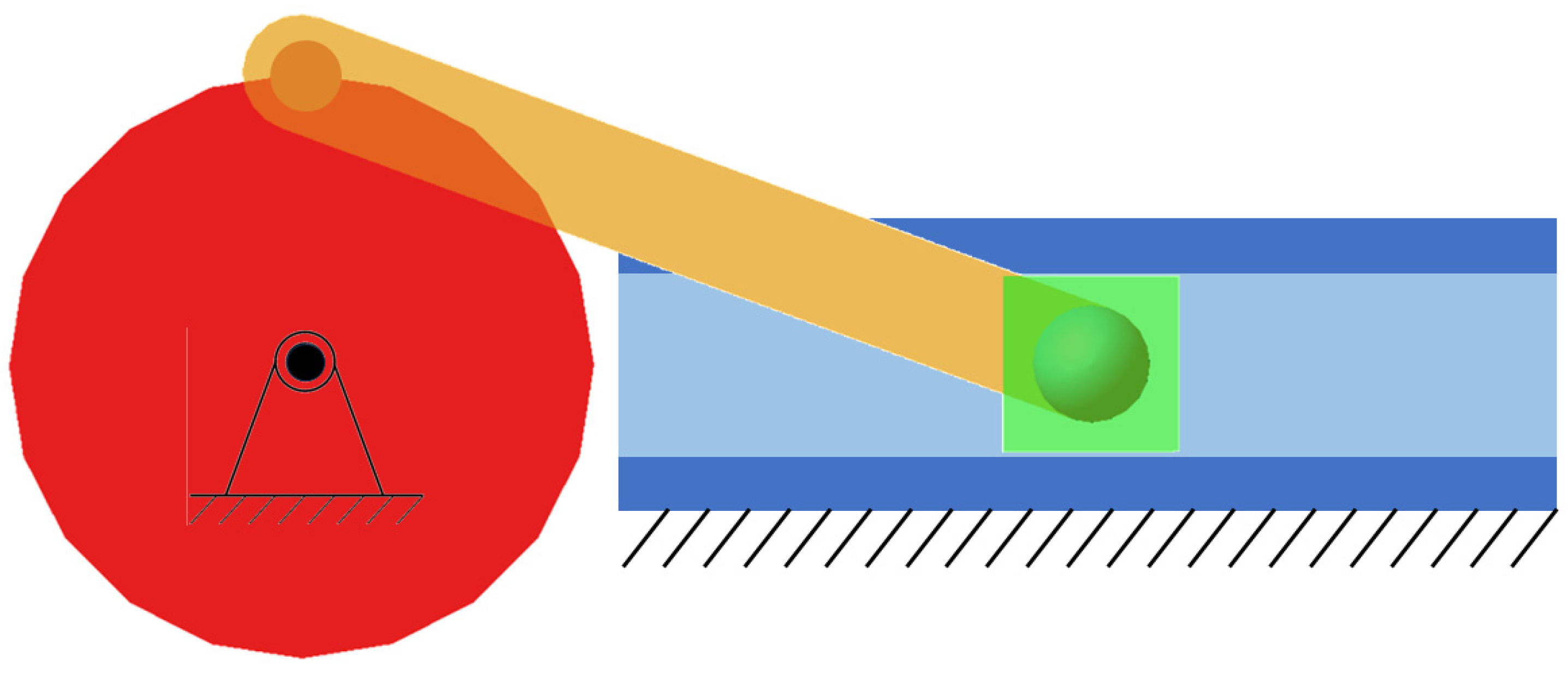
The crank–slider mechanism, illustrated in Figure 9, comprises four bodies: the frame, crank, connecting rod, and slider, with the frame expressed in the world reference frame. The mechanism includes one revolute joint, one spherical joint, one universal joint, and one translational joint, resulting in a single degree of freedom (DOF) according to the Chebychev–Grübler–Kutzbach criterion [34].

One of the objectives of this case study is to investigate the behavior of the translational joint. Therefore, although the DBD formulation does not suffer from over-constraint or singularity issues, identical joint types were selected for both the DBD and MBD models to ensure a consistent comparison. Since the universal joint is modeled as two revolute joints, a spider body was introduced, as described in Section 2.4.2. The revolute joint connects the crank to the frame, the spherical joint connects the connecting rod to the crank, and the universal joint connects the slider to the connecting rod through two revolute joints: one between the connecting rod and the spider body, and one between the spider body and the slider. The translational joint connects the slider to the frame.

The MBD model was constructed in two configurations. In the first configuration, all joints are represented as ideal kinematic constraints. In the second configuration, the joints are represented using the DBD formulation through sets of spring–damper elements, except for the translational joint, which remains modeled as a constraint. Representing the translational joint using the DBD formulation is non-trivial, and addressing this challenge may significantly increase the simulation time.

The mechanism is driven by a constant torque of 0.05 N·m applied to the crank during the first two seconds of the simulation. The properties of the bodies are summarized in

Table 1. Crank-slider mechanism’s body properties.

Body	Mass [kg]	Inertia [kg·m2]	Characteristic Dimensions [m]
Crank	1.2331	1.5413 × 10−3	Radius of 0.05
Connecting rod	0.113	1.9612 × 10−4	Length of 0.144
Slider	0.9813	4.0885 × 10−4	Cube, 0.03 × 0.03 × 0.03
Spider	0.025	4 × 10−6	Sphere, radius of 0.01

.

3.3.2. Four-Bar Mechanism

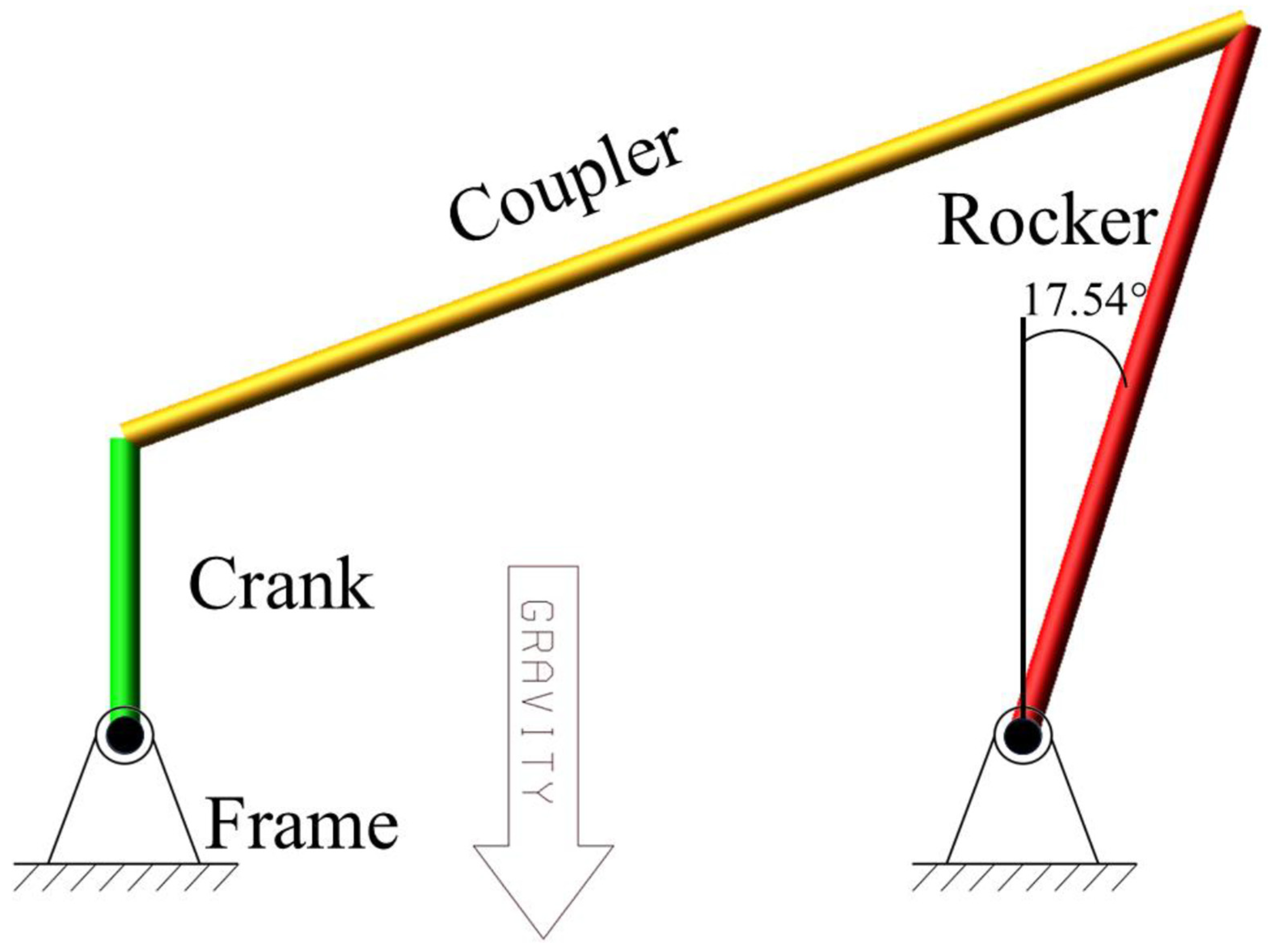
The four-bar mechanism, illustrated in Figure 10, comprises four bodies: frame, crank, coupler, and rocker, with the frame expressed in the world frame. The properties of these bodies are detailed in

Table 2. Four-bar mechanism’s body properties.

Body	Mass [kg]	Inertia [kg·m2]	Length [m]
Crank	1	8.333 × 10−2	1
Couple	1	1.333	4
Rocker	1	0.521	2.5

. In the MBD model, the mechanism consists of two revolute joints, one spherical joint, and one cylindrical joint, allowing for one degree of freedom as per the Chebychev–Grubler–Kutzbach criterion [34]. In contrast, all joints in the DBD model are revolute, as outlined in Section 2.4.1, due to the absence of over-constrained or singularity situations. In the DBD solver, joints are represented solely by forces generated through TSDAs, avoiding the need for traditional constraint equations.

A torsional spring of 50,000 Nm/rad is applied at both the crank-frame and rocker-frame joints. The crank-frame spring has a 10,000 Nm preload, while the rocker-frame spring has zero preload.

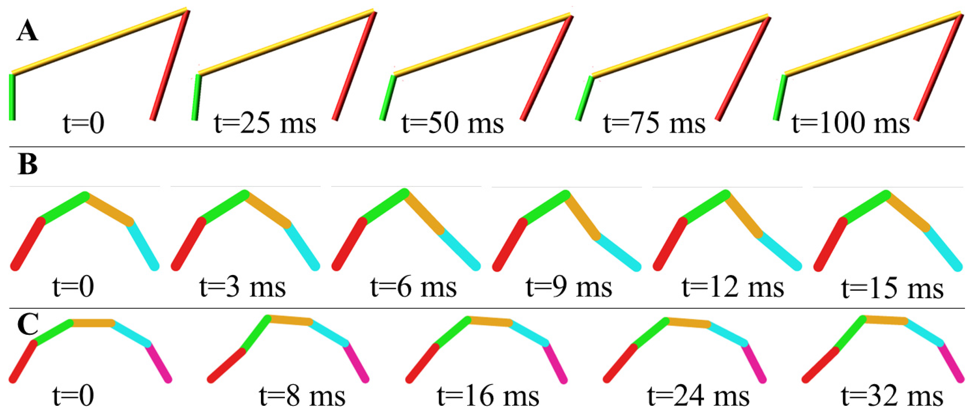
3.3.3. Five-Bar Mechanism (Topology A)

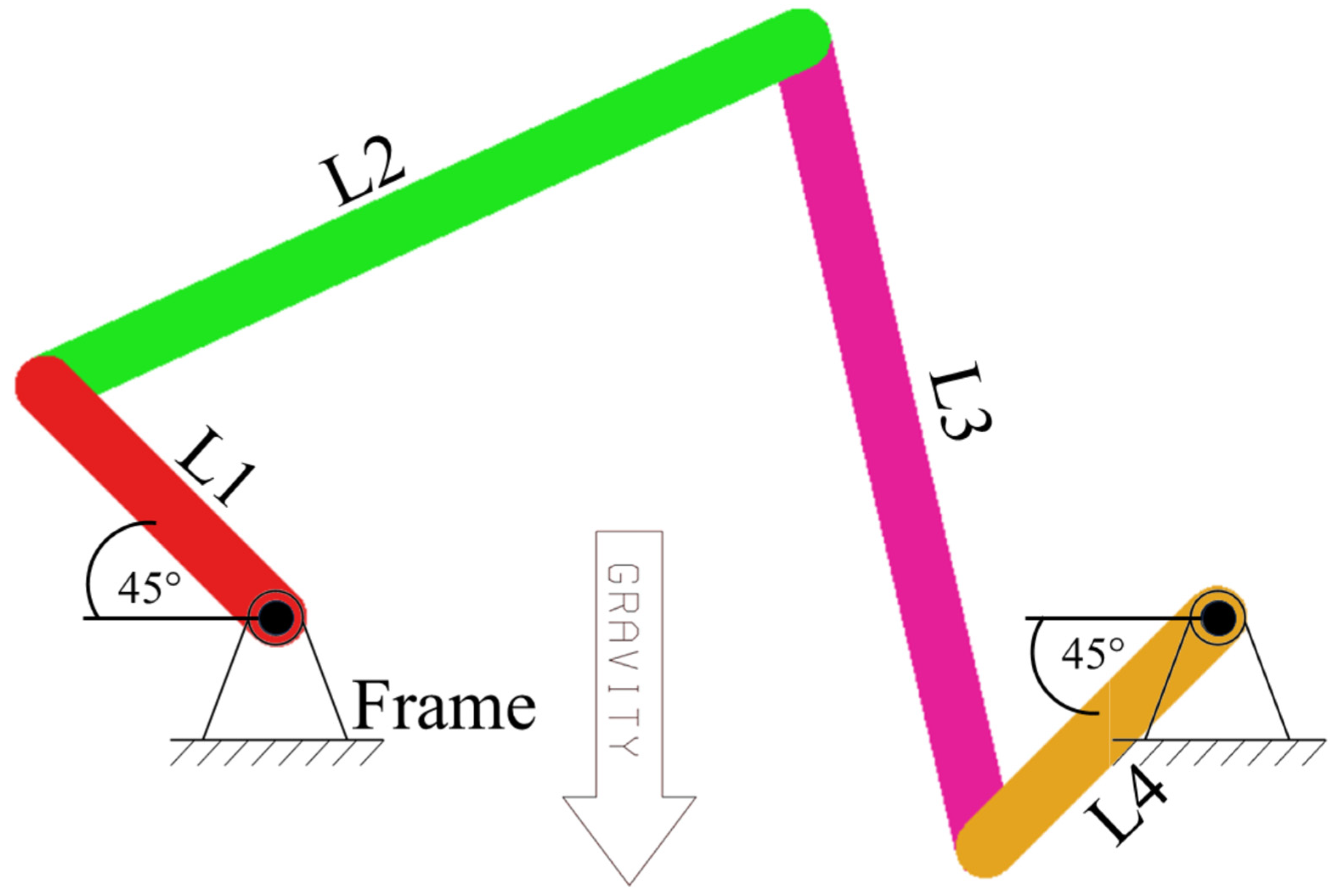
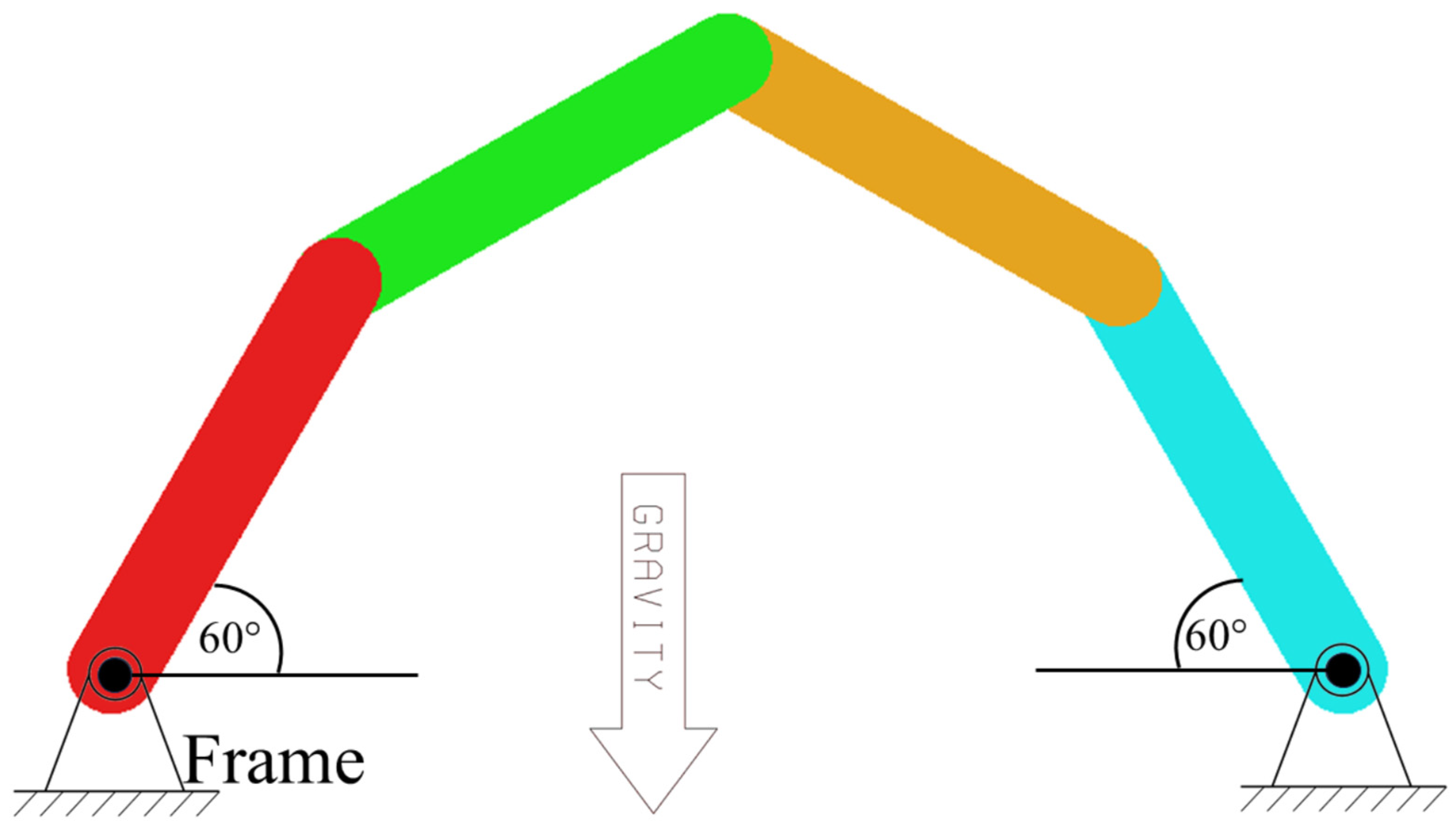
The five-bar mechanism, illustrated in Figure 11, consists of five rigid links, where the base link serves as the ground link, associated with the fixed world frame. This mechanism can be realized in two distinct topologies (see Figure 11 and Figure 12), which differ in the links’ lengths and in the spatial arrangement of the links relative to a horizontal reference line. In the first topology (topology A), the links extend across both sides of the reference line, resulting in an asymmetric structure. In the second topology (topology B), all links are positioned on the same side of the reference, forming a continuous, arc-like structure. These topological variations have a direct impact on the kinematic behavior, range of motion, and dynamic response of the mechanism. This subsection focuses on Topology A, while Topology B is discussed in the following subsection.

The properties of these bodies are detailed in

Table 3. Properties of the Five-bar mechanism in topology A.

Body	Mass [kg]	Inertia [kg·m2]	Length [m]
L1	1.286	3.7 × 10−3	0.16
L2	3.016	4.66 × 10−2	0.4064
L3	3.016	4.66 × 10−2	0.4064
L4	1.286	3.7 × 10−3	0.16

. In the MBD model, the mechanism consists of three revolute joints, one spherical joint, and one cylindrical joint, allowing for two DOF as per the Chebychev–Grubler–Kutzbach criterion [34]. To enable a direct comparison with the DBD formulation, the MBD model was also constructed using bushing elements at the joints, providing compliant behavior similar to the spring-damper representation used in the DBD approach. In contrast, all joints in the DBD model are revolute, as outlined in Section 2.4.1, due to the absence of over-constrained or singular configurations.

Torsional springs of 50,000 Nm/rad are applied at both the L1-frame and L4-frame joints. The L1-frame spring has a 10,000 Nm preload, while the L4-frame spring has zero preload.

3.3.4. Five-Bar Mechanism (Topology B)

The five-bar mechanism (topology B), illustrated in Figure 12, comprises five bodies with the frame belonging to the world. The properties of these bodies are detailed in

Table 4. Body properties: five-bar (topology B) and six-bar mechanisms.

Property	Value
Length [m]	0.3
Mass [kg]	6.5
Ixx = Izz [kg·m2]	0.07
Iyy [kg·m2]	0.003

. In the MBD model, the mechanism consists of three revolute joints, one spherical joint, and one cylindrical joint, allowing for two DOF as per the Chebychev–Grubler–Kutzbach criterion [34]. To enable a direct comparison with the DBD formulation, the MBD model was constructed using bushing elements at the joints. Each bushing was defined by linear translational springs, with a stiffness of 9 MN/m assigned to each individual spring component. No damping was included in the bushing definition. In contrast, all joints in the DBD model are modeled as revolute joints, as outlined in Section 2.4.1, since the mechanism does not involve over-constrained or singular configurations.

Torsional springs of 50,000 Nm/rad are applied at both the left bar-frame and right bar-frame joints. The left bar-frame spring has a 10,000 Nm preload, while the right bar-frame spring has zero preload.

3.3.5. Six-Bar Mechanism

The six-bar mechanism, illustrated in Figure 13, comprises six bodies with the frame belonging to the world. The properties of these bodies are detailed in Table 4. In the MBD model, the mechanism consists of three revolute joints, one spherical joint, and one cylindrical joint, allowing for two DOF as per the Chebychev–Grubler–Kutzbach criterion [34]. To enable a direct comparison with the DBD formulation, the MBD model was constructed using bushing elements at the joints. Each bushing was defined by linear translational springs, with a stiffness of 9 MN/m assigned to each individual spring component, and no damping was included. In contrast, all joints in the DBD model are modeled as revolute joints, as outlined in Section 2.4.1, since the mechanism does not involve over-constrained or singular configurations.

Torsional springs with a stiffness of 50,000 Nm/rad are applied at the leftmost (bar 1-frame) and rightmost (bar 5-frame) joints. The bar 1-frame spring is preloaded by 10,000 Nm, whereas the bar 5-frame spring has no preload. An additional torsional spring of 50,000 Nm/rad is connected between bars 4 and 5, while all other joints remain without torsional springs.

3.3.6. 3RRR Mechanism

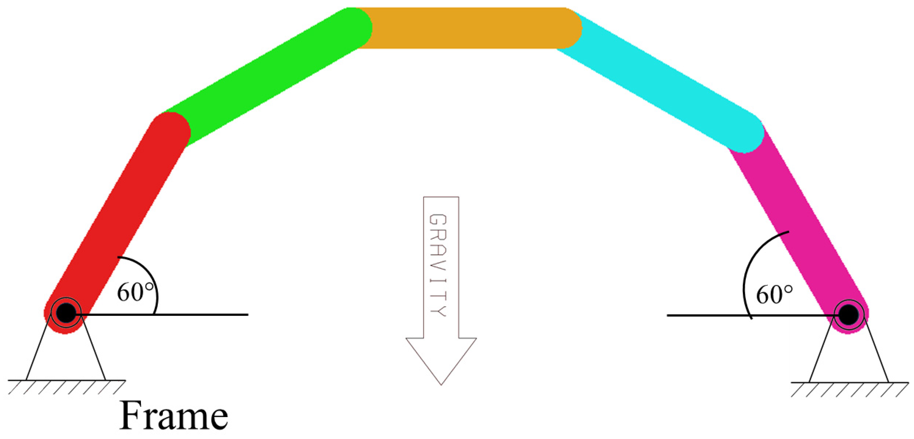
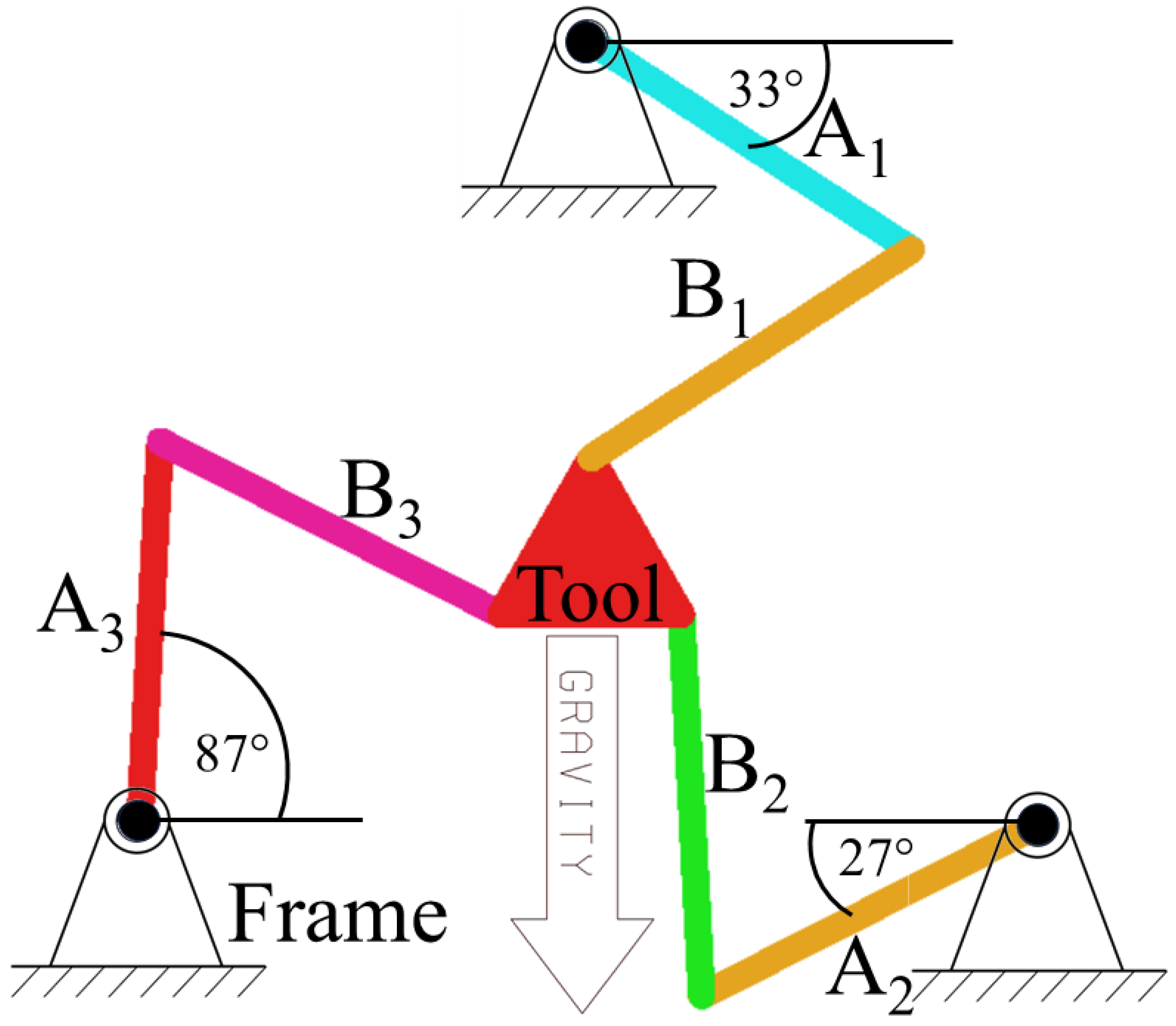
The 3RRR mechanism, illustrated in Figure 14, comprises eight bodies with the frame belonging to the world. The properties of these bodies are detailed in

Table 5. 3RRR mechanism’s body properties.

Body	Mass [kg]	Inertia [kg·m2]	Length [m]
A1	4	0.15	0.55
A2	4	0.15	0.55
A3	4	0.15	0.55
B1	4	0.15	0.55
B2	4	0.15	0.55
B3	4	0.15	0.55
Tool	23	0.015	0.26 side length

. In the MBD model, the mechanism consists of six revolute joints and three spherical joints, allowing for three DOF as per the Chebychev–Grubler–Kutzbach criterion [34]. In contrast, all joints in the DBD model are revolute, as outlined in Section 2.4.1, due to the absence of over-constrained or singular configurations.

Each frame-arm connection has a torsional spring with a stiffness of 50,000 Nm/rad. The torsional spring connecting arm A1 to the frame is preloaded by 10,000 Nm, whereas the torsional springs connecting arms A2 and A3 to the frame are unloaded.

To expand the mechanism types and to explore the impact of the number of bodies on the solver performance, this mechanism is also utilized with link A3 removed and link B3 connected to the world via a passive revolute joint at the original location, referred to as the 3RRR* mechanism. Further, when this modification is applied to link A2 as well, it is denoted as the 3RRR** mechanism.

3.3.7. 3RUU Mechanism (Delta Robot)

The 3RUU mechanism (typically known as the Delta robot [35]), illustrated in Figure 15, comprises 14 bodies with the frame belonging to the world. The properties of these bodies are detailed in

Table 6. 3RUU mechanism’s body properties.

Body	Mass [kg]	Ixx[kg·m2]	Iyy[kg·m2]	Izz[kg·m2]	Length [m]
A1	8.5	0.2	0.2	3 × 10−3	0.524
A2	8.5	0.2	0.2	3 × 10−3	0.524
A3	8.5	0.2	0.2	3 × 10−3	0.524
B1	20	2.5	2.5	6.5 × 10−3	1.244
B2	20	2.5	2.5	6.5 × 10−3	1.244
B3	20	2.5	2.5	6.5 × 10−3	1.244
Spider1A	0.5	1.4 × 10−4	1.4 × 10−4	1.4 × 10−4	-
Spider2A	0.5	1.4 × 10−4	1.4 × 10−4	1.4 × 10−4	-
Spider3A	0.5	1.4 × 10−4	1.4 × 10−4	1.4 × 10−4	-
Spider1B	0.5	1.4 × 10−4	1.4 × 10−4	1.4 × 10−4	-
Spider2B	0.5	1.4 × 10−4	1.4 × 10−4	1.4 × 10−4	-
Spider3B	0.5	1.4 × 10−4	1.4 × 10−4	1.4 × 10−4	-
Tool	1.5	8.2 × 10−4	8.2 × 10−4	1 × 10−3	-

. In the MBD model, the mechanism consists of 15 revolute joints (each universal joint modeled by two revolute joints), allowing for three DOF as per the Chebychev–Grubler–Kutzbach criterion [34]. The revolute joints in the DBD model are defined as outlined in Section 2.3.1, and the universal joints are defined as outlined in Section 2.4.2.

Each frame-arm connection, initially oriented horizontally with respect to the world frame, includes a torsional spring with a stiffness of 5000 Nm/rad. The torsional springs at the A1-frame and A2-frame connections are preloaded by 1000 Nm, while the torsional spring at the A3-frame connection is preloaded by −1000 Nm.

This mechanism is also utilized with link A3 removed and link B3 connected to the world via a passive revolute joint at the original location referred to as the 3RUU* mechanism. Further, when this modification is applied to link A2 as well, it is denoted as the 3RUU** mechanism.

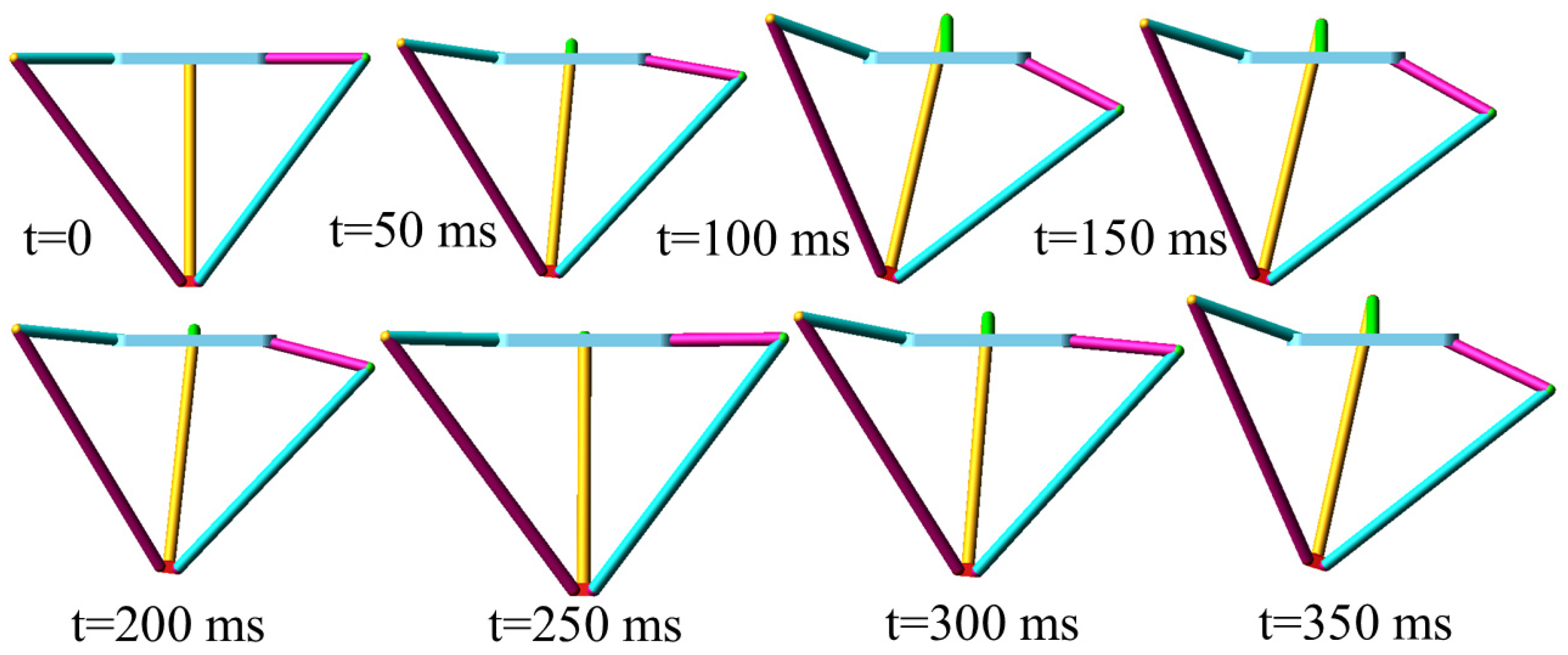
To provide a visual sanity check of the spatial topology and joint implementation, Figure 16 shows a pose montage of the 3RUU mechanism obtained in ADAMS at representative time instants. The snapshots illustrate the expected spatial motion and are provided for qualitative validation only.

4. Results and Discussion

4.1. Influence of the Number of Bodies and Constraints

The duration of a single time step, τ, is directly influenced by the number of bodies and constraints within the model. As the quantity of bodies and constraints increases, the duration of a single time step also increases. To provide a quantitative analysis of this phenomenon, we conducted time-step duration measurements across ten different systems (refer to

Table 7. (a) Number of equations of various systems. (b) Time of a single step as a function of the no. of bodies and TSDAs.

(a)
System Number	System Description	No. of Equations (MBD)	No. of Equations (DBD)
#1	Four-bar mechanism (the frame link expressed in the world frame)	35	18
#2	Five-bar (frame link expressed in the world frame)	46	24
#3	3RRR** (Section 3.3.6)	59	30
#4	3RRR* (Section 3.3.6)	70	36
#5	3RRR	81	42
#6	3RUU** (Section 3.3.7)	131	66
#7	3RUU* (Section 3.3.7)	142	72
#8	3RUU	153	78
#9	Two separate 3RUU systems	306	156
#10	Three separate systems: twice system #8 and one system #3	365	186
(b)
System Number	No. of Bodies	No. of TSDAs	τ [ms]
#1	3	24	0.267
#2	4	30	0.270
#3	5	42	0.284
#4	6	48	0.301
#5	7	54	0.304
#6	11	66	0.406
#7	12	78	0.423
#8	13	90	0.430
#9	26	180	0.626
#10	31	222	0.692

) that are various configurations of the four case-study mechanisms. The total number of equations in MBD is determined by the number of bodies and the constraints applied. Each body contributes six equations (three for translational motion and three for rotational motion), and additional equations are introduced based on the DOF restricted by the constraints. For example, consider the five-bar mechanism, which includes five bodies (four links and the frame, with the frame associated with the world body) and the following joints: three revolute joints, one spherical joint and one cylindrical joint. A revolute joint restricts five DOFs (allowing rotation about one axis), so for three revolute joints, 3 × 5 = 15 DOFs are constrained. A spherical joint restricts three DOFs (allowing free rotation about all three axes) and introduces three constraints. A cylindrical joint restricts four DOFs (allowing one translational and one rotational DOF), contributing four additional constraints. Thus, the total number of constrained DOFs is 15 (revolute) + 3 (spherical) + 4 (cylindrical) = 22 constrained DOFs. Thus, the total number of equations can be calculated as the sum of six equations for each body (6 per body for 4 bodies) plus the number of constrained DOFs: 6 × 4 (equations for bodies) + 22 (constrained DOFs) = 46 equations.

In contrast, with the DBD method, the system remains fully described by six equations for each body, as constraints are inherently handled by the interaction between elements. Therefore, the number of equations in DBD is 6 × 4 = 24 equations.

Figure 17 shows the duration of a single time step, τ, as a function of the number of equations for both ADAMS and the DBD method. Additionally, the figure displays τ for the DBD method after normalization by factor F (represented by the green line, DBD*). As expected, the duration of a single time step demonstrates a linear increase in the case of the DBD method, while the ADAMS formulation exhibits a second-order polynomial growth, as indicated by the red and blue lines in Figure 17. It is important to note that the complexity of solving the EOM in the MBD formulation is O(n³) regarding simplified numerical methods for solving linear systems of equations. To manage the computational load, sparse matrix techniques are often employed in solving large-scale linear systems of equations arising from MBD with constraints. However, as the number of coupling interactions between bodies increases, the sparsity of the matrix decreases, resulting in higher computational complexity.

Interestingly, the time-step duration for DBD initially surpasses that of ADAMS. Yet, when normalized by the previously identified factor, F (15.8, as found in Section 3.2), the time-step duration for DBD (represented by the green line, DBD*, in Figure 17) becomes shorter than that of ADAMS, even when considering the correction factor proposed by Aruoba et al. [33]. The total simulation time is given by τ·T/h where h is the time step size and T is the simulation end time. To accurately compare the efficiency of these methods, it is necessary to explore the factors influencing the time step size h, which we will address in a later section of this article.

To express the per-step runtime as a function of both problem size measures, we fitted a linear model $\tau =c+a n_{\mathrm{bodies}}+b n_{\mathrm{TSDAs}}$ using the benchmark data (Table 7b), obtaining $\tau \left[\mathrm{m}\mathrm{s}\right]=0.2175+0.0298 n_{\mathrm{bodies}}-0.0020 n_{\mathrm{TSDAs}}$ with RMSE $=0.0077$ ms (n = 10). The negative sign of $b$ is an artifact of the fit (strong correlation between $n_{\mathrm{bodies}}$ and $n_{\mathrm{TSDAs}}$ in this dataset); its small magnitude indicates that the TSDA contribution is negligible compared with the dominant $n_{\mathrm{bodies}}$ term, consistent with a linear scaling form $O(n_{\mathrm{bodies}}+n_{\mathrm{TSDAs}})$.

4.2. The Influence of Frequency on Time Step Size (In the DBD Method)

As expected, an increase in stiffness or the frequency spectrum within a dynamic system results in a smaller time step size. Our investigation involved various mechanisms with diverse body weight ratios (ranging from 1 to 40) and different frequencies (100–8000 Hz) achieved through a spectrum of spring constants (0.2–1000 MN/m). In Figure 18, the maximum allowable time step size is depicted as a function of frequency. Apart from the four-bar mechanism, all systems exhibit a favorable alignment with the relation h = ((2π)²f[Hz])⁻¹, showing an average error of 5.44% between the larger calculated time step size and the size obtained from the established relation.

On the other hand, the four-bar mechanism demonstrates a favorable alignment with the relation h = (2πf[Hz])⁻¹, showing an average error of 1.53% between the larger calculated time step size and the size obtained from the established relation. The distinction with the four-bar mechanism lies in the fact that each link’s movement is intricately tied to the movement of all other links. However, in the other systems, the movement of a specific link does not necessitate movement in all other links. Therefore, the convergence process in solving the dynamics of the four-bar mechanism is more efficient.

4.3. The Impact of Step Time Size and Stiffness on Accuracy

The computational challenges associated with solving the dynamics of closed-chain systems with more than three bodies using Lagrangian formulation or RNE have been recognized [18]. Accordingly, a high-accuracy numerical reference was defined as the DBD solution obtained with very high stiffness (k = 5 × 10⁸ N/m) and a very small time step (h = 5 × 10⁻⁹ s). To evaluate accuracy, an error metric was defined as the average offset of the tool body center position of the 3RRR mechanism (Figure 14), relative to the reference solution.

Table 8. The influence of time step size and system stiffness on the accuracy.

Spring Const. [N/m]	Frequency [Hz]	h	Error [mm]
2 × 106	337	7.52 × 10−5	3.1
2 × 106	337	1 × 10−5	3.1
2 × 106	337	1 × 10−6	3.1
2 × 106	337	1 × 10−7	3.1
5 × 106	524	4.85 × 10−5	1.2
5 × 106	524	1 × 10−5	1.2
5 × 106	524	1 × 10−6	1.2
5 × 106	524	5 × 10−7	1.2
5 × 106	524	1 × 10−7	1.2
5 × 107	1656	1.5 × 10−5	0.12
5 × 107	1656	1 × 10−6	0.11
5 × 107	1656	5 × 10−7	0.11
5 × 107	1656	1 × 10−7	0.11
5 × 108	5137	4.6 × 10−6	2.0 × 10−5
5 × 108	5137	1 × 10−6	5.6 × 10−6
5 × 108	5137	1 × 10−7	5.3 × 10−7
5 × 108	5137	5 × 10−8	2.5 × 10−7
5 × 108	5137	5 × 10−9	Reference

presents the errors in relation to the natural system frequency and time step size, h, of the 3RRR mechanism. The larger time step size corresponds to the maximum allowable, as outlined in Section 4.2.

Upon reviewing Table 8, it becomes evident that the time step size has a minimal impact on solution accuracy, whereas the system’s stiffness (frequency) exerts a significant effect.

4.4. Functional Evaluation of the Crank-Slider Mechanism and Its Joints

This section evaluates the performance of the crank–slider mechanism (Section 3.3.1) under the DBD formulation by examining both the global dynamic consistency of the system and the behavior of the mechanism’s joints during motion. The assessment includes a direct comparison with an equivalent multibody dynamics (MBD) model implemented in MSC ADAMS under two configurations. Specifically, ADAMS is used in two tiers: (i) an ideal-joint configuration using standard constraint-based joints (Section 4.4.1) and (ii) a model-equivalent configuration in which the joints are implemented to match the DBD TSDA (spring–damper) realizations as closely as possible (Section 4.4.2; the translational-joint exception is documented there).

All damping elements were removed to create an energy-conservative reference case. Under these conditions, the evolution of the total mechanical energy provides a global measure of numerical accuracy for both DBD and MBD solutions.

In addition to the energetic analysis, the local fidelity of the mechanism’s joints is evaluated using explicit kinematic measures, with particular attention to the translational joint behavior.

These findings indicate that the DBD method effectively preserves both the global dynamics and the intended joint relationships of the crank–slider mechanism, affirming its suitability for analyzing mechanisms with mixed joint types under dynamic loading.

To maximize the numerical accuracy of the ADAMS reference solution, the solver tolerance was set to Error = 1 × 10⁻¹⁰, which is the smallest tolerance value for which ADAMS successfully converged for the present model.

4.4.1. Comparison Between DBD and ADAMS with Ideal Constraint Joints

This subsection compares the performance of the DBD solver with the MSC ADAMS solver when the joints in the ADAMS model are represented as ideal kinematic constraints. Although the DBD method is inherently designed for compliant joint representations, this comparison provides an important reference case for assessing numerical accuracy and stability under extreme dynamic conditions.

In both models, all damping elements and frictional effects were removed, resulting in energy-conservative systems. Under these conditions, any variation in total mechanical energy reflects purely numerical dissipation or injection. The crank–slider mechanism was selected as a stress-test benchmark due to its severe operating conditions, including rapidly increasing velocities, large joint forces, and the presence of kinematic singular configurations.

During the simulation, the crank reaches angular velocities of approximately 30 rad/s (≈287 rpm), generating joint reaction forces of about 150 N. Since the mechanism includes bodies with very small mass and inertia, down to 0.04 kg, very stiff springs are required in the DBD formulation to closely approximate ideal joint behavior. Accordingly, a spring stiffness of 0.476 MN/m was assigned to each individual translational spring–damper element defining the joint, resulting in a dominant natural frequency of approximately 820 Hz for the joint representation.

Both simulations were executed for a total physical duration of 10 s. The driving torque was applied only during the first 2 s of the simulation, after which the system evolved freely under its inertial and elastic dynamics. The total computational runtime of the ADAMS simulation was 1.33 s. After applying the computational adjustment factor introduced in Section 3.2, the effective runtime of the DBD simulation was also 1.33 s, enabling a fair comparison in terms of numerical efficiency. The energy dissipation rate obtained with the ADAMS solver was approximately 0.2 mJ/s, whereas the DBD solver exhibited a higher dissipation rate of approximately 0.8 mJ/s. It is important to note, however, that the total mechanical energy introduced into the system during the simulation is approximately 1.8 J, exceeding the observed dissipation rates by more than three orders of magnitude in both cases.

A fundamental difference between the two approaches lies in their time-step control mechanisms. The ADAMS solver employs adaptive time stepping, where the step size is reduced in the vicinity of kinematic singularities and under rapid changes in joint forces. In contrast, the DBD solver is insensitive to singular configurations and force magnitudes, with its stability governed primarily by the dominant frequencies of the system.

Figure 19 presents the time-step size in the ADAMS simulation as a function of the crank angle. The red and blue curves represent the upper and lower envelopes of the scattered data, while the dashed black curve denotes the average time-step size. The color scale corresponds to the normalized crank angular velocity. The abrupt rise in the upper envelope reflects the adaptive step-size controller behavior around singular regions: the solver reduces the step near 0° and 180° but may increase it aggressively immediately after exiting these regions when the estimated local error drops. While this does not necessarily imply instability, it may reduce local fidelity (e.g., smoothing fast transients) and introduce convergence/phase artifacts; in practice it can be mitigated by imposing a maximum step-size bound (globally or within a crank-angle window), tightening the error tolerance, or adjusting integrator settings.

Overall, this comparison highlights a fundamental trade-off between constraint-based and constraint-free formulations. While the ADAMS solver achieves slightly lower numerical energy dissipation when ideal constraints are employed, this accuracy is obtained at the cost of adaptive time-step reductions driven by singular configurations and changing force levels. The DBD solver, although exhibiting somewhat higher numerical dissipation under extreme stiffness conditions, maintains stable integration without sensitivity to singularities. These results suggest that the DBD method is particularly well suited for systems operating under uncertain or highly variable conditions, as well as for mechanisms that inherently pass through singular configurations.

In this case, particular attention is given to evaluating the constraint fidelity of the translational joint within the DBD formulation. The root mean square (RMS) displacement of the slider from its nominal translation axis is 9.5 μm, while the RMS rotation about this axis is approximately 0.01 μrad.

These micrometer-scale deviations are consistent with typical clearance levels used in plain (sliding) bearings. According to ISO 12129-1 [36], recommended mean relative bearing clearances for plain bearings lie in the range ψ_m = 0.56–3.15‰. For representative sliding interface dimensions of 5 mm and 10 mm, this corresponds to absolute clearances of approximately 3–16 μm and 6–32 μm, respectively. The obtained RMS displacement therefore falls well within the range of physically realistic clearances for translational sliding interfaces.

4.4.2. Comparison Between DBD and ADAMS with Compliance Joints

Figure 20 presents a quantitative comparison between the DBD solver and the ADAMS (MBD) solver for the crank–slider mechanism investigated in this section, considering a system with compliant connections. The DBD values of simulation time/real-world time are reported after applying the study-specific scaling factor F (Section 3.2). Using a different F would shift the DBD curve horizontally along the SRT axis (right for smaller F, left for larger F), without changing the curve shape or the reported energy/accuracy trends. To ensure a consistent basis for comparison, the ADAMS model was constructed to resemble the DBD formulation as closely as possible: all connections were represented using linear springs, with no damping or friction included. Each spring defining the compliant connections was assigned a stiffness of k = 4 × 10⁵ N/m. The only modeling difference between the two approaches concerns the translational joint of the slider, which is naturally implemented in DBD using the same compliant formulation as the other connections, whereas in ADAMS it was defined as an ideal kinematic constraint due to practical limitations in defining an equivalent compliant representation.

As established in Section 4.2, the selection of the integration time step in DBD is based on a practical criterion derived from the dominant dynamic characteristics of the system. For the present mechanism, which is characterized by a dominant frequency of approximately 750 Hz, this criterion leads to a recommended time step of approximately 33.8 μs.

Figure 20 shows that in the vicinity of this recommended value, the DBD results exhibit a clear accuracy plateau, in which the rate of energy loss remains low and nearly constant over a relatively wide range of time steps. Within this plateau, the energy-loss rate obtained with DBD is on the order of ${\dot{E}}_{\mathrm{D}\mathrm{B}\mathrm{D}}\approx (5-7)\times {10}^{-3} J/s$, and displays only weak sensitivity to further reductions in the time step. This behavior defines a practically relevant operating region, where a favorable balance between numerical accuracy and computational cost is achieved.

However, Figure 20 also shows that in DBD, reducing the time step to values significantly smaller than the recommended one leads to a renewed increase in the measured energy-loss rate. This behavior is not unique to DBD but is also observed in ADAMS, indicating that beyond the plateau region the system dynamics are likely governed by mechanisms that are no longer associated with time-discretization errors. For very small time steps, the measured energy loss is influenced by the high sensitivity of the system to minute perturbations in the vicinity of kinematic singular configurations (dead-center positions), where the kinematic transmission ratio becomes ill-conditioned. As a result, the numerical response exhibits behavior that can be interpreted as effective stochasticity, in which numerical energy dissipation does not decrease monotonically with decreasing time step.

It should be noted, however, that in DBD a sufficiently large further reduction in the time step may, in some cases, lead to an additional decrease in the energy-loss rate, approaching nearly an additional order-of-magnitude reduction. This observation suggests that DBD retains the capability for further accuracy improvement through time-step refinement beyond the plateau, albeit at the cost of increased sensitivity to stochastic effects and higher computational effort.

In contrast, the ADAMS results do not exhibit a similarly well-defined plateau. As illustrated in Figure 20, reducing the effective time step or tightening solver settings in ADAMS does not result in a consistent improvement in energy conservation. Instead, the energy-loss rate tends to saturate at values of the same order of magnitude, often with larger variability, despite a substantial increase in computational cost. This behavior may be attributed to the enforcement of the translational joint as a kinematic constraint, which introduces additional stabilization mechanisms and associated algorithmic dissipation that are not directly controlled through the time-step size.

To make the ADAMS model equivalence and qualitative motion transparent, Figure 21 provides representative ADAMS snapshots exported from the same simulation run used to generate Figure 20.

Overall, Figure 20 demonstrates that for a stiff crank–slider mechanism with kinematic singularities, DBD provides a more favorable accuracy–efficiency trade-off. Near the recommended time step derived in the previous chapters, DBD achieves a stable low-dissipation plateau while also allowing for further accuracy improvements through time-step reduction. ADAMS, on the other hand, approaches comparable energy-loss levels only at significantly higher computational cost and without a systematic reduction in numerical dissipation as the time step is decreased.

4.5. MBD vs. DBD Solver Performance for Compliant Joints

For all comparisons in Section 4.5 and Section 4.6, the ADAMS models use the same compliant joint realizations as DBD (TSDA/spring-based), so that differences reflect solver behavior rather than joint idealization. This section evaluates solver performance for compliant joints in terms of accuracy and solution speed. Without a definitive analytical solution, the comparison will be based on energy loss. To achieve this, all dampers and external forces are removed to create an energy conservation system. In the following comparison, the rate of energy loss is calculated as the time derivative of the system’s total energy, where the total energy is the sum of the kinetic energy (based on the velocities of the bodies) and the potential energy (determined by the bodies’ heights and the energy stored in the springs).

This investigation was performed on the same topology to cancel the topology effect. The mechanisms examined include a four-bar mechanism (Section 3.3.1), a five-bar mechanism (Figure 12 and Table 4), and a six-bar mechanism (Figure 13 and Table 4). All mechanisms have a natural frequency of approximately 550 Hz. To provide a qualitative visualization of the three benchmark mechanisms and their motion, Figure 22 shows representative ADAMS snapshots for the four-bar (A), five-bar (Topology B) (B), and six-bar (C) mechanisms at selected time instants.

Figure 23 presents energy loss as a function of the SRT, where unity represents real-time execution and values below unity indicate FTRT simulation. Although MBD demonstrates superior FTRT performance, this advantage comes at the cost of solution accuracy, particularly when energy loss rates become substantial. Critically, this degradation occurs without explicit error indicators, potentially leading MBD to produce non-physical results. The three MBD curves show a very high rate of energy loss at high-speed solutions (low SRT). As SRT increases, the rate of energy loss decreases and eventually becomes constant at high SRT values. The maximum SRT for the MBD curves was obtained when the MBD solver failed, indicating a limit in the accuracy of the MBD solver. As the number of bodies increases, solver performance (both accuracy and solution speed) decreases.

However, the DBD solver demonstrates better performance, with the number of bodies having no direct influence on its performance. The DBD solver performs better when solving the five-bar mechanism compared to the four-bar mechanism, which may be explained by load path and distribution. The increased coupling between the mechanism bodies can make numerical challenges. As the number of bodies increases, this coupling effect weakens. Furthermore, the mechanism topology also influences coupling. This effect will be investigated in the following section.

The DBD solver achieves better performance than the MBD solver. The DBD solver yields good results even at the lowest possible SRT. Additionally, there is no lower boundary on the time step size for the DBD solver, and accuracy increases as the time step size decreases. When the SRT for the four-bar mechanism is 4310, the rate of energy gain decreases to 6.07 μJ/s.

4.6. The Topology Impact on the Solvers’ Performance

The topology of a mechanism, which refers herein to the arrangement of its components, plays a crucial role in determining its dynamic behavior. The arrangement of links in kinematic chains affects how motion and forces propagate through the mechanism. For instance, in a four-bar mechanism, the motion of one link predictably influences the entire mechanism due to full coupling. Additionally, the topology dictates the distribution of loads and forces across the mechanism, impacting both static and dynamic performance, including vibration propagation and response to external forces. To quantitatively characterize the impact of the mechanism topology, we introduce a new parameter called the Kinematic Topology (KT) value. This value is calculated using the root mean square (RMS) of the angular velocity ratio between the link connected to the frame without preloading, ${\omega }_{{out}_{rms}}$, and the link connected to the frame with preloading, ${\omega }_{{in}_{rms}}$:

$$KT={\displaystyle \frac{{\omega }_{{out}_{rms}}}{{\omega }_{{in}_{rms}}}}.$$

(11)

This investigation was performed on the five-bar mechanism with two different topologies. The first topology (Topology A) is the mechanism detailed in Section 3.3.2. Representative ADAMS pose snapshots of Topology A at selected time instants are provided in Figure 24 to visualize the qualitative motion used in this study. The second topology (Topology B) is shown in Figure 12 and Table 4. Both mechanisms have an approximate natural frequency of 550 Hz. The KT value for topology A is 2.77, while for topology B it is 1.13.

Figure 25 illustrates energy loss as a function of SRT. High KT decreases solver performance in both DBD and MBD methods. Additionally, high KT causes the constant rate of energy loss in MBD at high SRT to be higher. The DBD solver demonstrates better performance and can improve accuracy by increasing SRT.

This section highlights the significant impact of mechanism topology on solver performance, emphasizing the importance of considering KT in the analysis of dynamic behavior. The results indicate that mechanisms with higher KT values present more challenges for solvers, particularly for MBD, while the DBD solver shows greater robustness and accuracy under varying conditions.

4.7. Computational Trade-Offs Between DBD and MBD

Under what conditions does the DBD method have an advantage over the MBD method?

The answer depends on several factors. For both the DBD and MBD methods, of course, the number of bodies in the system is a crucial factor. For MBD, the number of constraints and the time step size used, and for the DBD, the system’s stiffness (or natural frequency). Since the time step in MBD is not known a priori and is dynamically updated during the simulation, it is challenging to provide a definitive answer. However, one can estimate the average time step in MBD that would result in an overall simulation time comparable to that of the DBD method.

Based on the curve-fitting equations shown in Figure 17 and Figure 18, a logarithmic graph was constructed (Figure 26). This graph was generated by applying the equations to a range of system parameters: natural frequencies from 10 Hz to 10,000 Hz; systems composed of 20 and 50 bodies; and varying numbers of constraints, ranging from an average of two constraints per body to five constraints per body.

The horizontal axis represents the natural frequency of the system (as modeled in DBD), while the vertical axis shows the MBD time step required to achieve the same total simulation duration as the DBD method. The graph exhibits a logarithmic slope, i.e., for each order-of-magnitude increase in frequency, the required MBD time step decreases accordingly to maintain equivalent computational effort. This implies that as the system’s natural frequency increases or as the number of bodies decreases, the MBD method can use smaller time steps.

These results suggest that the DBD method is more suitable for systems characterized by a large number of bodies and relatively low natural frequencies. For example, in the case of a MacPherson suspension system, the first natural mode of the bushings is approximately 20 Hz, while the sixth mode reaches about 250 Hz [37]. An MBD model of such a suspension system comprising 20 bodies would require an average time step of approximately 0.55 ms to match the total simulation time of an equivalent DBD simulation.

Further examples of stiffer systems include four-, five-, and six-bar mechanisms (see Figure 10, Figure 11, Figure 12 and Figure 13), where the system stiffness results in vibrations around 500 Hz. For these mechanisms, the MBD method requires a time step of approximately 0.13 ms to achieve the same simulation duration as DBD. However, if the goal is to preserve the same rate of energy dissipation, the MBD time step would need to be reduced to approximately 2 μs.

5. Conclusions

This paper investigates the performance of the DBD solver for closed-chain mechanisms and compares it with the ADAMS/View solver. Previous research on open-chain mechanisms reported improved accuracy for the DBD solver under the tested conditions [18]. In the present closed-chain benchmark suite, DBD shows a favorable accuracy-efficiency trade-off, reflected by lower energy drift over a broad range of time-step sizes and stiffness values.

In the tested cases, the main observed advantages of the DBD solver, particularly under pronounced dynamic effects, are:

• Accuracy (energy drift): Across the examined cases, DBD generally exhibits lower numerical dissipation than ADAMS/View at comparable computational effort and provides a practical time-step selection criterion based on the system’s dominant natural frequency.
• Runtime behavior: For a given accuracy target, DBD can achieve favorable simulation speed; however, the advantage depends on system stiffness (dominant natural frequency), problem size, and constraint density.
• Time-step refinement: DBD can attain very high accuracy by decreasing the time step, with the practical limitation being computational cost and available hardware resources.
• Applicability and stiffness regime: The advantage of DBD is most pronounced in compliant (flexible) joint/system realizations (e.g., rubber bushings), where the dynamics are governed by spring-based interactions. As the system becomes increasingly stiff and approaches an ideal-constraint regime, variable-step MBD solvers can become comparatively more efficient.

Overall, the results suggest that the relative benefit of DBD tends to increase with the model size and constraint density in the examined benchmarks and that DBD can offer an attractive option for complex closed-chain systems with significant dynamics.

Based on the benchmark suite presented in this paper, the DBD formulation is most suitable for:

• Closed-chain mechanisms with compliant joint realizations, where joints are naturally represented by spring/TSDA elements (e.g., bushings, elastokinematic suspensions, clearance-like behavior, and mechanisms where small compliance is physically justified).
• Systems dominated by moderate natural frequencies, for which an explicit time step satisfying the dominant-frequency criterion (Section 4.2) remains practical, including cases that benefit from uniform fixed-step integration and predictable stability behavior.
• Highly constrained topologies where constraint-driven solver behavior (adaptive step reductions, constraint stabilization, and sensitivity near singularities) can dominate the runtime/accuracy trade-off in classical DAE-based MBD solvers.
• At the same time, DBD has clear limitations:
• High-frequency/hyper-stiff regimes: If joint stiffness is increased to approach ideal constraints, the dominant natural frequencies rise and explicit integration requires very small time steps, making runtime potentially prohibitive; in such cases, variable-step stiff DAE solvers can be more efficient.
• Real-time constraints: Real-time or faster-than-real-time execution with DBD is feasible primarily when the dominant frequencies are sufficiently low (or the compliance is sufficiently high) so that the required stable time step is not overly small.
• Modeling intent: DBD replaces ideal constraints by compliant realizations; therefore, when the physical system is truly rigid and high-frequency dynamics are essential, this compliant representation may be an approximation that must be justified (or complemented by an MBD reference).

Future work will explore the scalability of the DBD solver for contact and friction problems and their application in even more complex systems and its potential applications in various engineering fields, especially in the automotive and off-road fields.