AC Series Arc Fault Detection Method Based on Composite Multiscale Entropy and MRMR-RF

Abstract

Series arc faults often occur in aging or faulty electrical systems due to insulation degradation, poor contact, or corrosion. These faults typically generate low current signatures, which are difficult to detect with traditional overcurrent protection methods. To address this measurement challenge, this paper proposes a systematic fault detection framework that combines discriminative feature extraction, statistical validation, and optimized classification. To comprehensively characterize arc fault signals, a diverse set of time- and frequency-domain features is extracted, and composite multiscale entropy is introduced to quantify nonlinear and transient fault dynamics more effectively. The MRMR (Maximum Relevance Minimum Redundancy) algorithm is applied to select features with high information content and low redundancy, thereby improving model generalization. A random search algorithm is used to adaptively optimize the random forest hyperparameters, establishing a high-accuracy fault diagnosis model. The experimental setup was established based on the UL1699B standard using a 115 V/400 Hz arc fault platform, and 1800 sets of data under nine different load types were collected for training and validation. Experimental results show that the proposed method outperforms five mainstream machine learning algorithms in terms of fault detection accuracy and performance. The results confirm its metrological robustness and its potential for deployment in waveform-based fault electrical monitoring systems.

1. Introduction

With the increasing complexity of modern electrical systems across various sectors, including transportation and industrial applications, the risk of series arc faults is growing. These faults are commonly caused by insulation degradation, corrosion, or mechanical wear, and they can lead to overheating, equipment damage, or even fires. Among various arc types, series arc faults are particularly difficult to detect due to their low current characteristics, making them a significant focus in electrical safety and fault measurement research. In recent years, researchers have explored a variety of arc fault detection approaches, including methods based on physical arc phenomena, mathematical arc modeling, and signal analysis in the time and frequency domains. For example, Vasile and Ioana [1] introduced a dual-dimensional arc fault detection system based on electromagnetic and acoustic waves, enhancing fault detection accuracy and localization capability. Ge and Liu [2] used MATLAB to establish the Cassie arc model and, through differential equations, simulated the voltage and current waveforms, arc conductance, and heat dissipation power of arc faults under different types of loads to achieve accurate identification of such faults. Yang et al. [3] proposed a ring-shaped arc sensor based on electric field measurement, which detects arc faults through non-contact near-field induction, achieving an accuracy of approximately 80%. Miao et al. [4] established a multi-feature arc model to simulate arc current accurately and proposed an arc fault detection technique based on magnetic field induction and an autocorrelation algorithm.

Although sensor-based technologies and arc mathematical models can achieve high accuracy in detecting arc occurrences, they are often susceptible to environmental disturbances, making them less reliable in complex electrical environments. Consequently, detection methods based on time–frequency-domain features of current waveforms have been more widely adopted in academic research, as they are effective in capturing transient signal patterns caused by arc faults under controlled experimental conditions. Koziy, Kim and Zhang et al. [5,6,7] detect arc faults by comparing the time–frequency-domain features of fault current waveforms with predefined thresholds. For example, Reference [6] extracts peak-to-peak value and spectral integration as feature indicators and compares them with adaptive thresholds to detect arc faults. Zhang et al. [7] employs a discrete wavelet transform (DWT) for voltage transient event detection and current drop pattern recognition. By combining adaptive thresholding, peak detection, and repetition frequency calculation, these methods achieve efficient arc fault identification.

With the development of artificial intelligence, researchers have conducted diversified analyses and fusion of current data in both the time and frequency domains. The accuracy and reliability of arc fault detection have been significantly enhanced by training and recognizing patterns using machine learning classifiers and improved neural network models. For example, Cui, Zhao, and Yu et al. [8,9,10] employ classical support vector machine (SVM) methods. Fault features are extracted by integrating even and odd harmonic components with signal magnitude and optimizing VMD parameters. Fault diagnosis is performed using SVM optimized by particle swarm optimization (PSO) and least squares support vector machine (LSSVM) models, achieving fault identification accuracy exceeding 95%. However, SVM performs poorly in handling multi-class problems and struggles with high-dimensional feature scenarios.

As a result, the random forest model [11,12,13,14,15,16], which performs well in complex feature classification has been widely applied. Guo et al. [14] proposes a method based on multi-feature fusion and random forest, in which the parameters of the random forest algorithm are optimized to efficiently identify series arc faults. Tong et al. [15] proposes a random forest (RF) model optimized using the Time-Variance-Accuracy (TVA) coefficient to address the issue of feature aliasing in series arc fault identification under low-voltage power scenarios, achieving an accuracy of 98.096%. Dai et al. [16] introduces an effective L2/L1 norm to quantify the fluctuation of current signals during arc fault occurrences, and combines it with a random forest classifier to achieve an accuracy of 98.74% under varying load conditions.

In addition, various improved neural network models [17,18,19,20,21] have also been widely applied. Among them, Liu et al. [18] proposes an AC arc fault detection method based on FCM-LSTM-CNN. By introducing fuzzy C-means (FCM) clustering, the training complexity of the neural network is reduced, resulting in faster convergence and improved detection efficiency, achieving a detection accuracy of 96.95%. He et al. [21] proposes a series DC arc fault detection method that combines load classification with a lightweight convolutional neural network (CNN). This approach effectively addresses the issue of feature aliasing caused by different load types, achieving an accuracy of 96.67%. Although convolutional neural networks (CNNs) possess powerful feature extraction capabilities and can achieve high classification accuracy, their effectiveness often relies heavily on large-scale, high-quality labeled datasets and careful architecture tuning. In arc fault scenarios with limited data and high waveform variability, their performance may become unstable or overly sensitive to load diversity and noise, leading to higher measurement uncertainty. Additionally, CNNs typically require longer training times compared to traditional machine learning models. Therefore, when classification accuracy is comparable, random forest models offer a more metrologically robust and computationally efficient alternative [16].

In summary, existing research typically applies time–frequency-domain analysis to current waveforms and utilizes handcrafted or fused features as inputs to classifiers such as Support Vector Machines, Random Forests, and Convolutional Neural Networks, achieving high detection accuracy in conventional residential and industrial AC systems. However, these methods often assume ideal operating environments and may not generalize well to complex AC power systems. In such systems, strong electromagnetic interference, compact circuit layouts, and diverse load conditions cause arc current waveforms to exhibit high nonlinearity and variability. This significantly challenges fixed or manually designed feature selection strategies, often leading to feature redundancy, overfitting, increased measurement uncertainty, and limited generalization across diverse operating conditions.

To address these challenges, this paper proposes a structured detection framework for AC series arc faults that integrates composite multiscale entropy (CMSE), MRMR-based feature selection, and a Random Search–optimized Random Forest classifier. The CMSE representation enhances sensitivity to nonlinear and dynamic waveform characteristics, while MRMR reduces feature redundancy and improves generalization. Cross-validated hyperparameter optimization further ensures robustness and practical computational efficiency. The framework is applicable to quasi-periodic AC current signals with localized disturbances, covering both conventional 50/60 Hz systems and higher-frequency applications such as 400 Hz power networks.

Although entropy-based features and Random Forest classifiers have been previously employed in arc fault detection, most studies apply these techniques independently without systematically coupling multiscale representation, redundancy-aware selection, and classifier optimization within a unified pipeline. In contrast, the proposed CMSE–MRMR–RF framework establishes an integrated and interpretable measurement strategy tailored to complex arc current signals. This structured methodological integration, rather than the isolated use of entropy itself, constitutes the principal novelty of this study. The main contributions of this paper are summarized as follows:

(1)

A novel composite multiscale entropy approach is proposed, which integrates time- and frequency-domain features to comprehensively capture the dynamic and nonlinear characteristics of arc currents. Compared with traditional entropy measures, this method improves sensitivity to waveform complexity and enhances detection robustness, thereby reducing the uncertainty associated with fault signature measurement under variable operating conditions.

(2)

The Maximum Relevance Minimum Redundancy (MRMR) algorithm is adopted to perform data-driven feature selection, effectively reducing dimensionality and eliminating irrelevant or redundant features. This enhances the generalization ability and computational efficiency of the detection model in the presence of noise and varying load characteristics.

(3)

A Random Forest classifier is fine-tuned using a Random Search optimization strategy, employing stratified 5-fold cross-validation with F1-score as the objective function. This improves the model’s robustness, accuracy, and training efficiency, particularly under complex electrical environments with limited labeled data, ensuring consistent and reliable measurement outcomes.

(4)

The proposed method serves as a representative and effective example of a broader class of arc fault detection techniques that integrate time–frequency feature fusion with interpretable machine learning models. Unlike black-box neural networks, this framework combines transparent feature construction, statistical separability analysis (via Cohen’s d), and redundancy-aware selection, enabling both high detection performance and strong measurement interpretability. Its modular and computationally efficient design makes it suitable for academic exploration as well as practical deployment in real-time or resource-constrained fault monitoring systems, addressing the practical need for efficient measurement tools.

The remainder of this paper is organized as follows. Section 2 introduces the theoretical background, including the features in the time domain and in the frequency domain, the composite multiscale entropy, the MRMR algorithm, the Random Forest classifier, and the Random Search optimization method. Section 3 details the implementation of the proposed method. Section 4 presents experimental validation and analysis. Section 5 concludes the study.

2. Theoretical Background

2.1. Traditional Time- and Frequency-Domain Feature

Time-domain feature analysis is the most intuitive method in signal processing and forms the foundation for quantifying waveform characteristics. It primarily includes quantitative features (such as maximum, minimum, mean, peak-to-peak value, and variance) and dimensionless features (such as kurtosis, skewness, pulse factor, and margin factor). Quantitative features are sensitive to signal variations and can capture subtle differences, but their stability is relatively poor, often leading to higher measurement variance under noisy conditions. In contrast, dimensionless features exhibit stronger anti-interference capability and greater stability, providing more robust and reproducible metrics, making them more effective in reflecting the essential characteristics of the signal for diagnostic purposes.

The Pulse Factor (PF) effectively captures transient changes in the signal, as defined in Equation (1), where X_p is the peak value, X_i is the discrete sample value, and N is the total number of sampling points. The Margin Factor (MF) measures waveform fluctuation and distortion, as shown in Equation (2). Kurtosis (Kur) is highly sensitive to spike components in the signal and is commonly used to analyze waveform distortions and assess the presence of anomalous impulses, and its expression is shown in Equation (3), where X_i represents the sampled value of the signal, and N is the total number of sampling points. The Waveform Factor (WF) indicates how much the signal deviates from an ideal sinusoidal waveform, as presented in Equation (4). The time-domain features are summarized in

Table 1. Time-domain characteristic indexes.

Name	Formula	Serial Number
Pulse Factor	$PF={\displaystyle \frac{X_p}{\frac{1}{N}{\displaystyle \sum _{i=1}^N\left|x_i\right|}}}$	(1)
Margin factor	$MF={\displaystyle \frac{X_p}{{(\frac{1}{N}{\displaystyle {\sum }_{i=1}^N\sqrt{\left|X_i\right|}})}^2}}$	(2)
Kurtosis	$Kur={\displaystyle \frac{\frac{1}{N}{\displaystyle \sum _{i=1}^N{\left(x_i-\overline{x}\right)}^4}}{{\left(\frac{1}{N}{\displaystyle \sum _{i=1}^N{\left(x_i-\overline{x}\right)}^2}\right)}^2}}$	(3)
Waveform Factor	$WF={\displaystyle \frac{\sqrt{\frac{1}{N}{\displaystyle \sum _{i=1}^N{x_i}^2}}}{\frac{1}{N}{\displaystyle \sum _{i=1}^N\left|x_i\right|}}}$	(4)

.

Frequency-domain analysis of signals typically involves transforming time-domain signals into frequency spectra using the Fourier Transform or further deriving different frequency-domain representations such as energy spectrum, power spectrum, and cepstrum. Based on these representations, frequency-domain features listed in

Table 2. Frequency-domain characteristic indexes.

Name	Formula	Serial Number
Frequency Center	$FC={\displaystyle \frac{{\displaystyle \sum _{k=1}^N{f}_{k}P(f_k)}}{{\displaystyle \sum _{k=1}^{N}P(f_k)}}}$	(5)
Mean Square Frequency	$MSF={\displaystyle \frac{{\displaystyle \sum _{k=1}^N{f_k}^{2}P(f_k)}}{{\displaystyle \sum _{k=1}^{N}P(f_k)}}}$	(6)
Root Variance Frequency	$RVF=\sqrt{{\displaystyle \frac{{\displaystyle \sum _{k=1}^N{(f_k-FC)}^{2}P(f_k)}}{{\displaystyle \sum _{k=1}^{N}P(f_k)}}}}$	(7)

can be extracted. Among them, the frequency center (FC) indicates the dominant frequency component of the signal, representing where the signal power is concentrated (Equation (5)), providing a concise measure of the spectral centroid. The Mean Square Frequency (MSF) focuses on the signal’s energy distribution, reflecting its concentration and dispersion in the frequency domain (Equation (6)), which is crucial for assessing the stability of harmonic components. The Root Variance Frequency (RVF) measures the dispersion in the power spectral energy distribution, indicating the deviation of each frequency component from the FC (Equation (7)), where f_k denotes the frequency value, P (f_k) represents the power spectral density, and N is the total number of frequency points. RVF is particularly valuable for measuring the spectral broadening caused by transient faults, thereby quantifying the instability introduced into the system.

2.2. Composite Multiscale Entropy Feature

Entropy is a concept from thermodynamics used to describe the degree of chaos or disorder in a system. Based on this, Shannon proposed information entropy to quantify the uncertainty of information. Information entropy can measure signal complexity, where a higher entropy value indicates greater uncertainty. However, traditional information entropy only analyzes the characteristics of the original signal on a single time scale. For non-stationary signals like arc fault signals, which may exhibit rapid fluctuations over short time scales and slower trends over longer scales, traditional methods may overlook important signal information, resulting in incomplete characterization and high measurement uncertainty. To address this issue, Liu et al. 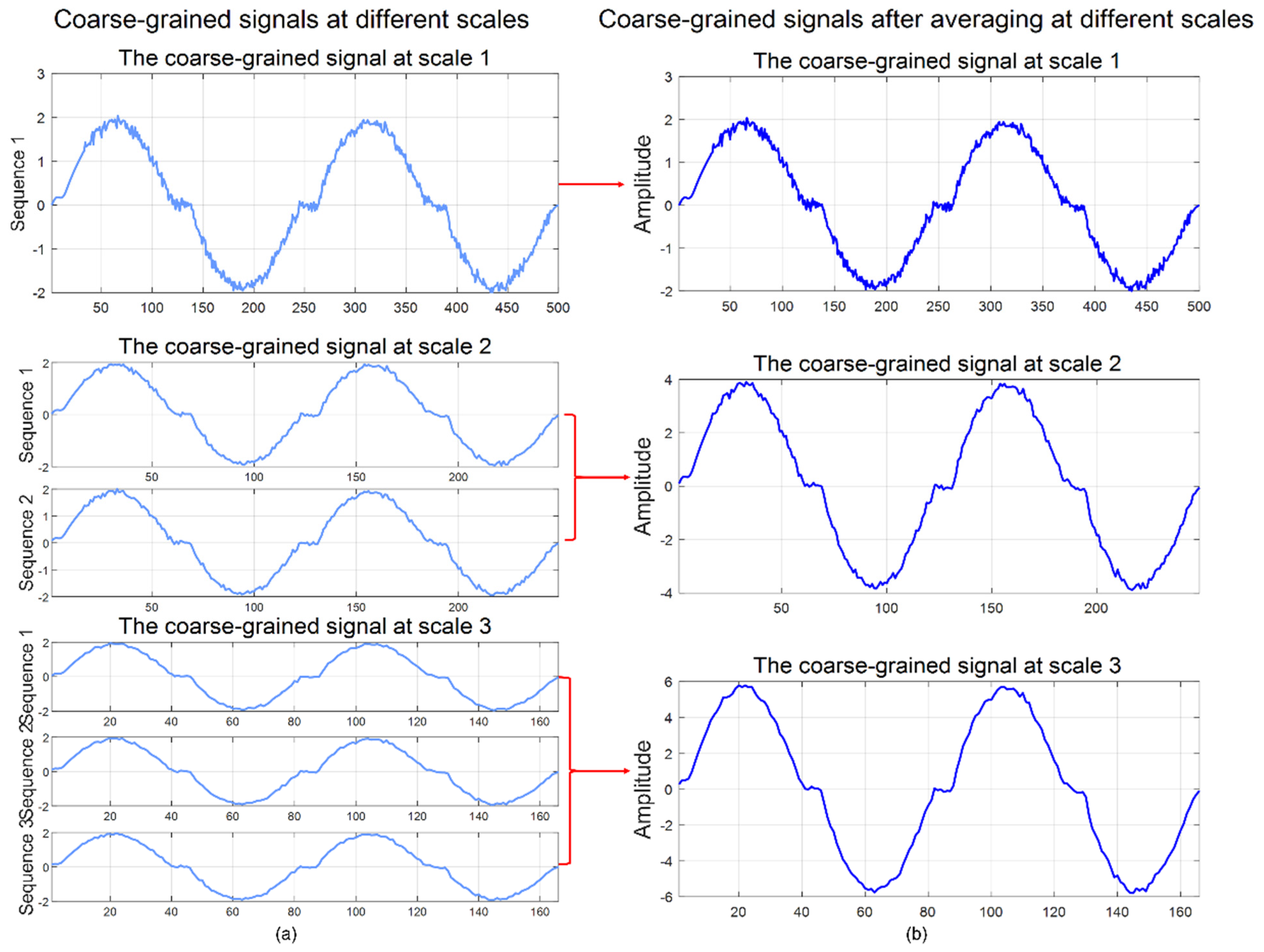[22] proposed a circuit fault feature extraction method based on Empirical Mode Decomposition (EMD) and Composite Multiscale Entropy. The method first performs coarse-graining on the original signal selecting a scale factor τ = n to generate n different coarse-grained sequences. Then, the entropy of each sequence is calculated, and the average of these values is taken as the composite multiscale entropy. This approach enhances both the precision of fault information extraction and the accuracy of entropy computation by providing a multi-resolution perspective, which significantly improves the robustness and stability of complexity measurement against noise and non-stationary behavior.

The calculation process of composite multiscale power spectrum entropy is as follows: First, perform a Fourier transform of the sub-signal at each scale to obtain its spectrum, and then calculate the power spectrum of the signal. Then, determine the proportion of the energy of each frequency point to the total energy to obtain the power spectral density P(f_k). Next, calculate the entropy of the power spectrum at each scale from the power spectral density, as shown in Equation (8). Finally, average the power spectral entropy across all scales to obtain the composite multiscale power spectrum entropy. This multi-scale averaging process yields a more reliable metric for the disorderliness of the power distribution across frequencies, reducing the volatility inherent in single-scale analysis.

$$H=-{\displaystyle \sum _{K=1}^{N}P(f_k)}\ln P(f_k).$$

(8)

The process of composite multiscale sample entropy extraction is as follows:

(1) Construct an m-dimensional vector X_m(i) = {p(i), p(i + 1), …, p(i + m − 1)} from the given data sequence {p(i), i =1, 2, …, N}. The distance d between vectors X_m(i) and X_m(j) is defined as the maximum absolute difference between their elements, as shown in Equation (9):

$$d={\max }_{k=0,1,\dots ,m-1}\left|p(i+k)-p(j+k)\right|$$

(9)

(2) For each i, count the number of instances where the distance between vectors X_m(i) and X_m(j) is less than or equal to the threshold r, and denote this count as B_i^m (r), and compute the average as B_i^m. For 1 ≤ i ≤ N − m, define B_i^m (r) and B_i^m as Equation (10):

$${B_i}^m(r)={\displaystyle \frac{1}{N-m-1}}{\displaystyle \sum _{j=1,j\ne i}^{N-m}\mathsf{\Theta }(r-d)}, B^m(r)={\displaystyle \frac{1}{N-m}}{\displaystyle \sum _{i=1}^{N-m}{B_i}^m(r)}.$$

(10)

where Θ (⋅) is the unit step function.

(3) Set m = m + 1 and repeat steps (1) to (4) to calculate B_{m + 1}(r). Then, the sample entropy of the original sequence is Equation (11):

$$SampEn(m,r,N)=-\ln {\displaystyle \frac{B^{m+1}(r)}{B^m(r)}}$$

(11)

(4) For multiple different scale sequences, repeat the above steps to obtain the sample entropy sequence {SampEn(τ)}. Perform averaging on the sample entropy across all scales to obtain the composite multiscale sample entropy. This composite measure effectively quantifies the temporal irregularity of the signal across multiple time resolutions, mitigating the risk of drawing conclusions from a single, potentially misleading, scale and thus enhancing the trustworthiness of the measurement.

The size of the sample entropy is mainly related to the dimension m and the threshold r. When m takes 1 or 2 and r takes 0.1–0.25 times the standard deviation (Std) of the data series, it has more reasonable statistical characteristics, offering a good trade-off between measurement accuracy and computational feasibility. In this paper, m = 2 and r = 0.2Std are selected as the parameters for calculating sample entropy to ensure statistically valid and reproducible entropy estimates.

2.3. Maximum Relevance Minimum Redundancy (MRMR) Feature Selection Algorithm

Maximum Relevance Minimum Redundancy (MRMR) is a mutual information-based filter method that selects features with strong relevance to the target class and low redundancy among themselves. In complex electrical systems, arc fault signals exhibit high nonlinearity and uncertainty due to environmental noise, circuit designs, and load variations, which complicate feature extraction and can degrade the performance of the measurement system. MRMR, which makes no assumptions about data distribution, provides a principled approach to quantifying the relevance to class labels and suppresses redundancy through mutual information, thereby improving model discrimination and generalization. This process is essential for constructing an efficient and reliable measurement feature set that minimizes information overlap and maximizes diagnostic signal, ultimately reducing the model’s complexity and vulnerability to overfitting. The implementation process is as follows [23]:

(1)

First, the mutual information I (f_i, f_j) between the i-th feature and the j-th feature is calculated, where each feature vector f_i = [f(i,1), f(i,2), …. f(i,m)] ^T contains m samples. The mutual information is defined as shown in Equation (12):

$$I(f_i,f_j)={\displaystyle \sum _{f_i,f_j}p(f_i,f_j)\log \frac{p(f_i,f_j)}{p(f_i)p(f_j)}}$$

(12)

where p (f_i, f_j) is the joint probability distribution of features f_i and f_j, p(f_i) and p(f_j) are their respective marginal probability distributions.

(2)

Let the output class be defined as O = [O₁, O₂, O₃, … O_m] ^T. The mutual information I (f_i, O) between each feature f_i and the output class O is calculated. For the current feature subset S, the average mutual information with the output is given by Equation (13):

$$D(S,O)={\displaystyle \frac{1}{\left|S\right|}}{\displaystyle \sum _{f_i\in S}I(f_i,O)}$$

(13)

(3)

Next, according to the minimum redundancy criterion, the average mutual information R(S) among features within the subset is computed, as shown in Equation (14):

$$R(S)={\displaystyle \frac{1}{{\left|S\right|}^2}}{\displaystyle \sum _{f_i,f_j\in S}I(f_i,f_j)}$$

(14)

(4)

By combining the objectives of maximum relevance and minimum redundancy, the optimized objective function in Equation (15) searches for an optimal feature subset $S$ from the original feature pool $F$. The maximization is performed over candidate subsets $S\subset F$, aiming to maximize the relevance $D\left(S,O\right)$ to the output labels while minimizing the redundancy $R\left(S\right)$ among the selected features.

In this study, a forward selection strategy is adopted to iteratively construct the feature subset that maximizes the objective function. The resulting subset represents a parsimonious yet highly informative feature space, effectively balancing measurement accuracy and computational efficiency for subsequent classification.

$$MRMR(S)=\max (D(S,O)-R(S))$$

(15)

2.4. Basic Framework of Random Forest

Random Forest is a commonly used ensemble learning algorithm that combines the Bagging strategy with Classification and Regression Trees (CART) to improve prediction accuracy and robustness, making it particularly suitable for measurement applications requiring high stability and repeatability. Its core idea is to build multiple decision trees trained on different subsets of the data and to make predictions through majority voting, thereby reducing model variance and enhancing generalization capability. This ensemble approach effectively averages out the uncertainties and errors of individual trees, leading to more consistent and reliable measurement outcomes. Specifically, given a training dataset with N samples and Y features, the algorithm first generates K data subsets of size M ≤ N using bootstrap sampling (i.e., sampling with replacement), and constructs one decision tree for each subset. During the construction of each tree, at each node, a random subset of X ≤ Y features is selected to determine the optimal split. Each decision tree grows independently until a stopping condition is met, such as a maximum tree depth or a minimum number of samples per leaf node. After training, all trees are used to predict the test samples, and the final output is determined by majority voting across all trees. By introducing randomness in both sample selection and feature selection, Random Forest effectively mitigates overfitting and improves its adaptability to various data distributions, ensuring robust performance even when measurement conditions or input data vary.

2.5. Random Search Algorithm Optimization Parameter Process

To achieve optimal model performance, hyperparameter tuning plays a crucial role. Among various tuning strategies, random search algorithms have shown higher efficiency in exploring high-dimensional parameter spaces due to their uniform sampling mechanism. Compared with traditional grid search, random search significantly reduces computational overhead while often discovering superior hyperparameter configurations within limited computational resources [24]. By randomly sampling combinations of hyperparameters, this approach minimizes reliance on specific parameter values and enhances the generalization capability of the model.

The implementation of random search involves first defining a range or a list of candidate values for each hyperparameter. Then, multiple hyperparameter combinations are sampled randomly from the defined space. For each combination, model performance is assessed using cross-validation or a separate validation set, commonly based on metrics such as accuracy or F1-score, thereby providing a statistically rigorous estimate of the model’s predictive performance. This process is repeated either for a predetermined number of iterations or until a set time constraint is met. Finally, the parameter set that achieves the best performance on the validation set is selected as the optimal configuration. This systematic tuning process minimizes the risk of suboptimal model configuration, ensuring that the final model delivers consistent and accurate measurements.

3. Methodological Implementation

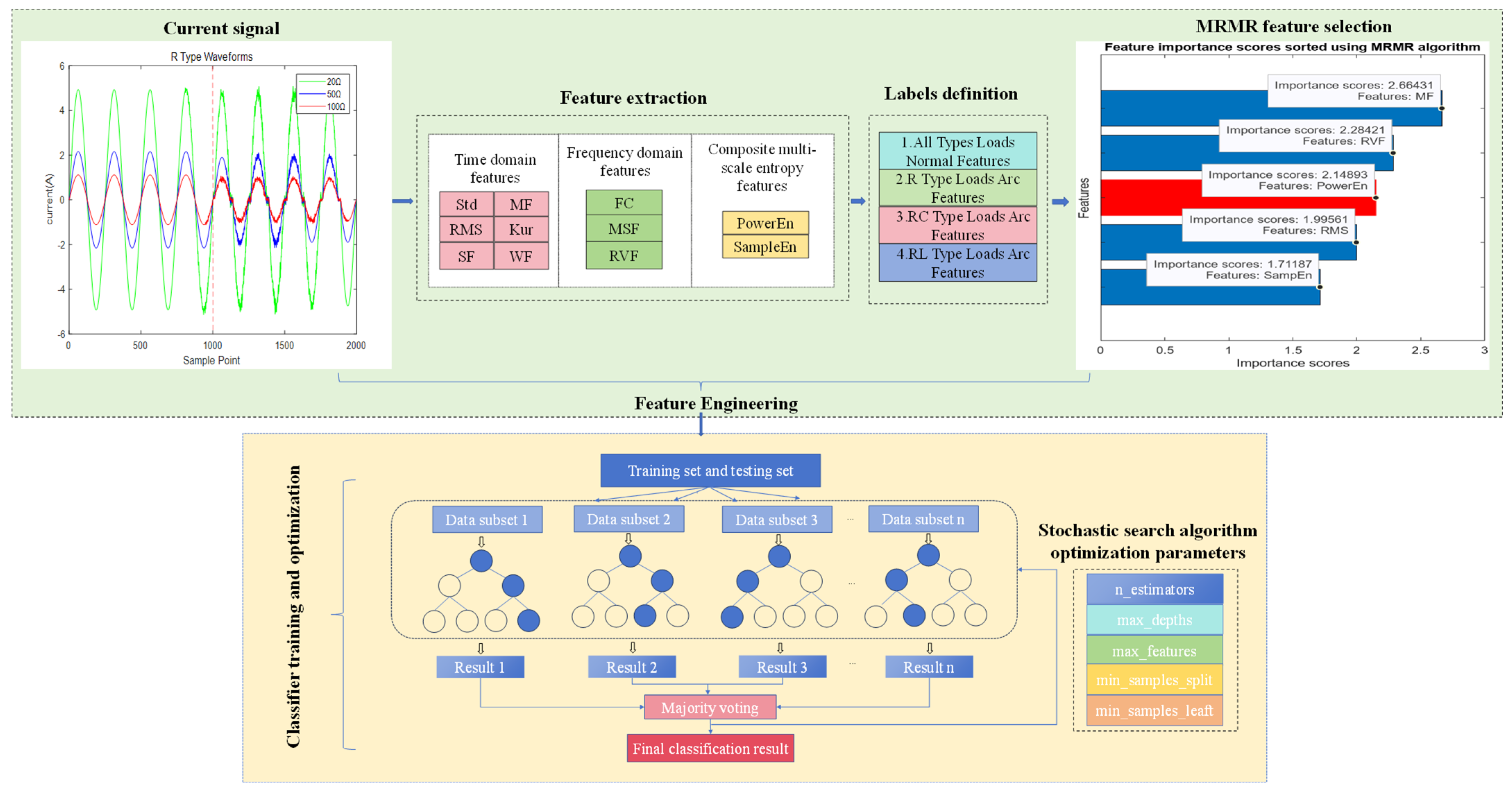
To accurately and efficiently identify series arc faults in complex electrical AC systems, this paper proposes a comprehensively improved arc fault detection method. The framework of the proposed method is shown in Figure 1. To comprehensively capture the dynamic characteristics of fault currents, multidimensional signal features are extracted and then filtered using the MRMR algorithm to construct a high-quality dataset. The random forest is then trained and tested on this dataset, and its key hyperparameters are optimized using random search to achieve not only accurate but also robust and reproducible arc fault identification.

3.1. Experimental Platform Construction

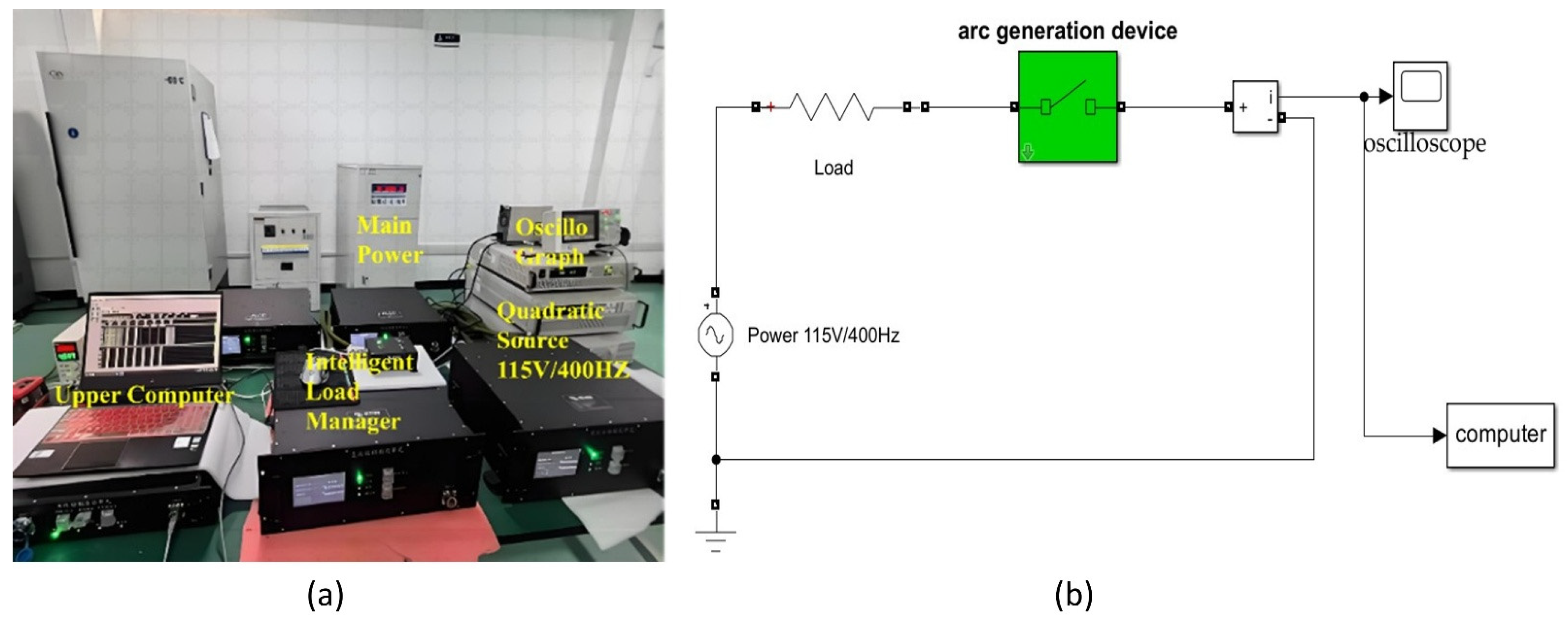
Considering the practical application requirements of intelligent power supply systems and the need for standardized and repeatable experimental measurements, this study establishes an arc fault experimental platform based on the UL1699B standard under controlled laboratory conditions to simulate arc faults under real-world conditions. The main components of the experimental platform include a power supply, an arc generation device, an intelligent load manager, an oscilloscope, and a computer, as shown in Figure 2. The AC power source is connected in series with the arc generation device and the adjustable load module. The current sensor is installed in series between the arc generator and the load to measure the line current waveform. The measured signal is transmitted to the digital oscilloscope and subsequently transferred to a computer for storage and analysis.

To comprehensively replicate actual application scenarios, the experiments are conducted under a power supply condition of 115 V/400 Hz using three primary load types: purely resistive loads simulating lighting and heating equipment, resistive–inductive loads representing motor-driven devices such as electric pumps, and resistive–capacitive loads representing switch-mode power supplies. These three load categories are selected as representative fundamental components of typical electrical systems and serve to characterize the essential transient behaviors of arc faults under both linear and partially nonlinear conditions. In particular, resistive–capacitive loads were selected to approximate the input characteristics of switch-mode power supplies as defined in UL1699B. To further enhance experimental realism, future work will incorporate actual nonlinear power electronic modules—such as AC-DC rectifiers, PWM inverters, and digitally controlled DC-DC converters—to emulate switching transients, harmonic distortion, and dynamic load behaviors more accurately. The specific load parameters are defined according to the UL1699B standard, as shown in

Table 3. Load types and parameter values.

Load Type	Parameter Size
Resistive Load	20 Ω ± 1%, 50 Ω ± 1%, 100 Ω ± 1%
Resistive–inductive Load	3 mH ± 10% + 30 Ω ± 1%, 3 mH ± 10% + 50 Ω ± 1%, 3 mH ± 10%H + 80 Ω ± 1%
Resistive–capacitive load	45 μF ± 5% + 20 Ω ± 1%, 45 μF ± 5% + 50 Ω ± 1%, 45 μF ± 5% + 100 Ω ± 1%

.

3.2. Data Collection

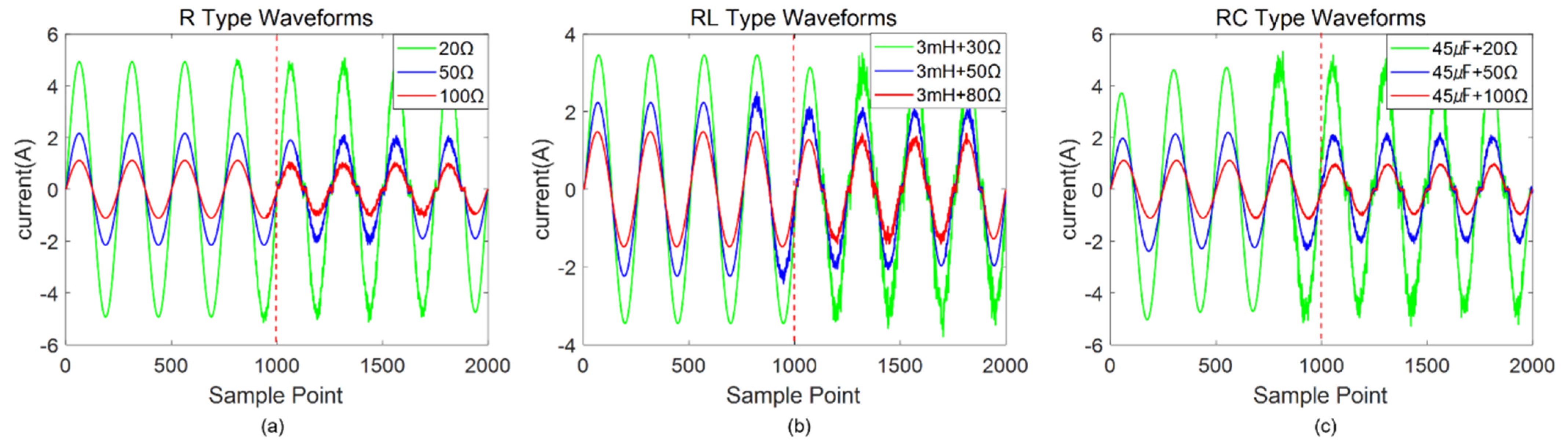
According to the setting of the experimental platform, the frequency of AC voltage is 400 Hz, and the period of the current waveform is 0.0025 s. In order to completely reflect the current signal characteristics, 500 sample points within two complete periods (0.005 s) are taken as one sample. The sampling frequency is set to 100 kHz, the sampling time of each load is set to 0.5 s, and a total of 100 samples is collected, and the signal is divided into two states: normal and faulty, so there is a total of 2 (states) × 9 (loads) × 100 (samples) = 1800 samples, while adding random noise to simulate the actual interference. As each load condition is equally sampled under both normal and fault states, the resulting dataset is balanced and does not require additional class imbalance handling or data augmentation. Figure 3 shows the sampled waveforms under the above nine different loads with different parameters. The left side of the red dotted line in the figure indicates the time-domain signal of the normal state, and the right side indicates the time-domain signal of the fault state. It can be seen that when a fault occurs, the peak current fluctuates and is accompanied by a ‘flat shoulder’ phenomenon, providing a visual validation of the distinct measurable characteristics induced by arc faults.

Although the time-domain signals show visible perturbations, it should be emphasized that the overall RMS current variation remains moderate and does not correspond to a high-current short-circuit condition. The pronounced “flat shoulder” phenomenon does not indicate an excessive current magnitude but rather reflects waveform distortion caused by the nonlinear voltage–current characteristics of arc discharge. Such nonlinearity introduces harmonic redistribution and temporal irregularity within each half-cycle.

While harmonic distortion indices (e.g., THD) are not explicitly calculated in this study, the increased signal complexity associated with harmonic redistribution is quantitatively captured through composite multiscale entropy and power spectrum entropy features. Therefore, the interpretability of the flat-shoulder phenomenon is supported not only by visual waveform observation but also by entropy-based complexity metrics embedded within the proposed framework.

3.3. Feature Extraction

3.3.1. Traditional Time- and Frequency-Domain Feature Extraction

To comprehensively and stably quantify the irregular fluctuations of waveforms during faults, this paper combines the advantages of both quantitative and dimensionless features and extracts the commonly used quantitative features such as standard deviation (Std) and root-mean-square (RMS), and the dimensionless features such as pulse factor (PF), margin factor (MF), kurtosis factor (Kur), and waveform factor (WF) as the time-domain features.

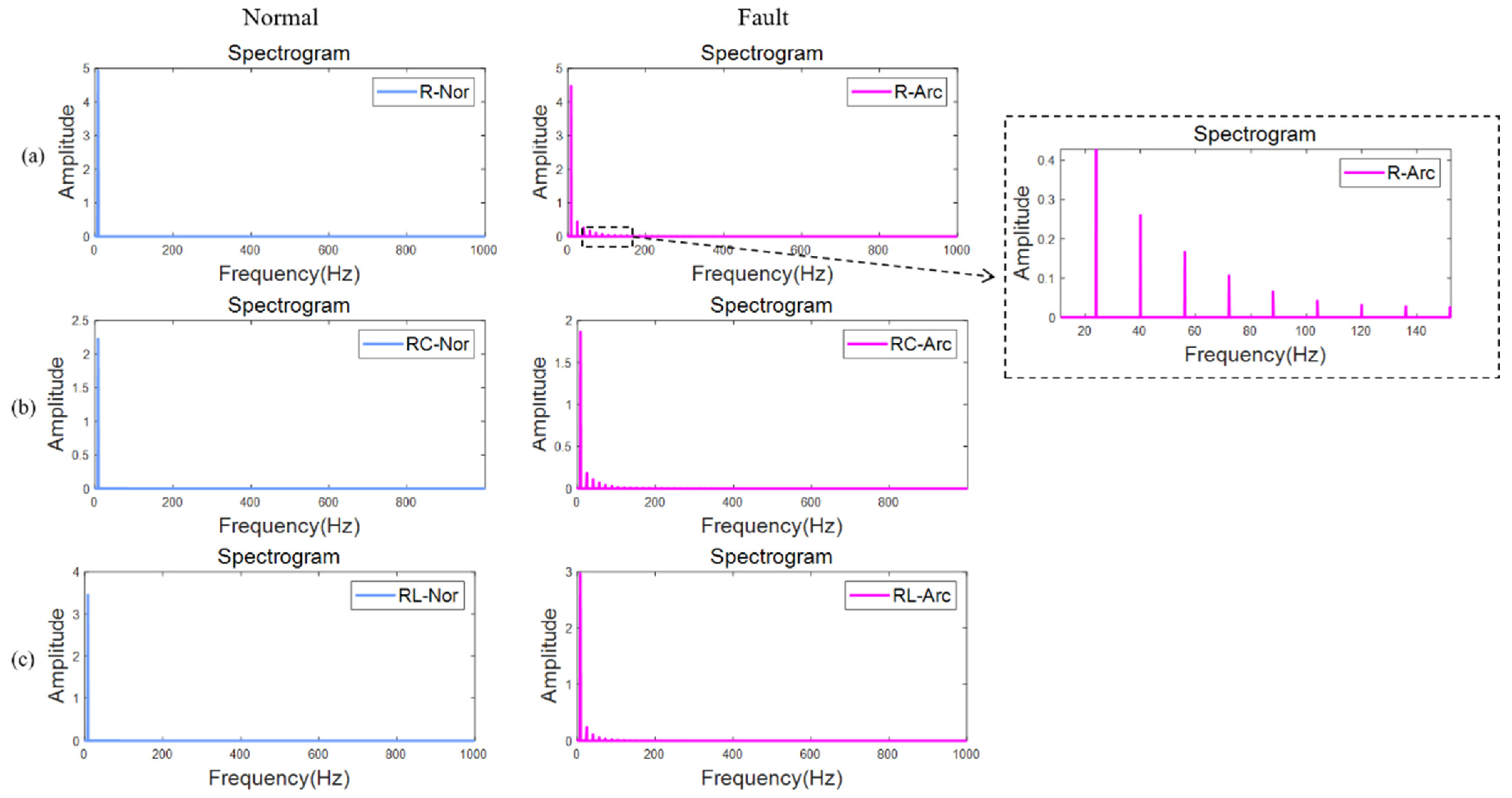
By analyzing the frequency spectra of the processed current signals under normal and fault conditions (Figure 4), it can be observed that the plotted spectra correspond to the preprocessed signals used for feature extraction rather than the raw 400 Hz supply waveform. To emphasize arc-induced fluctuations, the dominant 400 Hz fundamental component was attenuated during preprocessing. As a result, the remaining spectral energy is primarily distributed in the lower-frequency region (below approximately 150 Hz), where modulation effects and stochastic variations introduced by arc discharge become more pronounced.

It should be noted that the spectral resolution in Figure 4 is determined by the finite analysis window length (Δf = 1/T). The approximately 20 Hz component corresponds to the first non-zero frequency bin of the FFT and therefore reflects the discretization of the spectral analysis rather than a physical oscillation frequency of the arc process.

Under fault conditions, additional spectral components emerge and the energy distribution becomes more dispersed across the frequency band, demonstrating a clear spectral broadening effect. This redistribution of spectral energy is consistently observed across different load types, indicating the general nonlinear and time-varying characteristics induced by arc faults. Such behavior directly motivates the selection of frequency-domain indicators. Specifically, features such as Frequency Center (FC), Mean Square Frequency (MSF), and Root Variance Frequency (RVF) provide quantitative measures for characterizing spectral shift and dispersion. These indicators effectively capture the redistribution of harmonic energy while maintaining robustness under varying load conditions, thereby enhancing the reliability of the diagnostic framework.

3.3.2. Composite Multiscale Entropy Feature Extraction

To conduct a more comprehensive and detailed analysis of arc fault signal information, this paper will extract two key features: the composite multiscale power spectral entropy, which quantifies the complexity of energy distribution in the frequency domain and reflects changes in spectral structure caused by arc faults, and the composite multiscale sample entropy, which quantifies the irregularity of time-domain signals and captures the transient variation processes of arc faults. Compared with conventional statistical features, these entropy indicators offer a more comprehensive characterization of arc fault signals. Traditional features often operate on a single scale or fixed window, which may fail to capture the time-varying, nonlinear nature of arc discharges, leading to incomplete feature extraction and higher measurement uncertainty under variable operating conditions. In contrast, multiscale entropy aggregates information across multiple resolutions, enabling detection of both transient bursts and longer-term waveform fluctuations, thereby offering a more holistic and stable measurement of signal complexity. The dual use of sample and spectral entropy further enhances robustness by jointly reflecting temporal irregularity and spectral complexity, creating a more fault-resilient feature set.

Given the microsecond-level transient characteristics of arc pulses (ranging from 0.05 to 0.5 ms) and a sampling rate of 100 kHz, the scale factor τ was initially set within the range of 3 to 10 to ensure effective coverage of typical arc dynamic features. Under identical load parameters, nine sample groups were randomly selected from both normal and fault conditions. For each sample, composite multiscale power spectral entropy and composite multiscale sample entropy were computed across scale factors from τ = 3 to τ = 10.

To quantitatively assess the discriminative power and statistical significance of entropy features at different scales, this study introduces Cohen’s d, a widely used effect size metric. Cohen’s d measures the standardized difference between two means. It is defined as Equation (16):

$$d={\displaystyle \frac{\left|{\mu }_1-{\mu }_2\right|}{s_p}},s_p=\sqrt{{\displaystyle \frac{{s_1}^2+{s_2}^2}{2}}}$$

(16)

where μ₁ and μ₂ represent the mean values of a given feature under normal and fault states, respectively, and S₁ and S₂ denote their corresponding standard deviations. The pooled standard deviation S_p serves as a normalization factor. A higher value of Cohen’s d indicates a stronger discriminative capability of the feature at that specific scale [25]. As shown in

Table 4. Composite Multiscale Power Spectral Entropy Summary of Cohen’s d Calculations.

Scale (τ)	Normal Group Mean (M1)	Fault Group Mean (M2)	Cumulative Standard Deviation	Cohen’s d
Scale 3	1.1839	1.2922	0.048	2.26
Scale 4	0.2009	0.3028	0.052	1.96
Scale 5	0.9125	1.0126	0.042	2.38
Scale 6	1.1874	1.2830	0.045	2.13
Scale 7	1.3272	1.4204	0.039	2.39
Scale 8	1.4260	1.5178	0.038	2.42
Scale 9	1.5583	1.6493	0.040	2.28
Scale 10	1.6689	1.7555	0.041	2.11

and

Table 5. Composite Multiscale Sample Entropy Summary of Cohen’s d Calculations.

Scale (τ)	Normal Group Mean (M1)	Fault Group Mean (M2)	Cumulative Standard Deviation	Cohen’s d
Scale 3	0.1175	0.1614	0.012	3.66
Scale 4	0.1626	0.2148	0.016	3.26
Scale 5	0.2180	0.2704	0.018	2.91
Scale 6	0.2526	0.3093	0.021	2.70
Scale 7	0.2686	0.3333	0.023	2.81
Scale 8	0.2790	0.3482	0.025	2.77
Scale 9	0.2748	0.3624	0.028	3.13
Scale 10	0.2639	0.4122	0.042	3.53

, Cohen’s d effect sizes for both the composite multiscale power spectral entropy and sample entropy are significantly greater than 0.8 across all scales (τ = 3–10), with the minimum d = 1.96 and the maximum d = 3.66, far exceeding the threshold for a “large effect”. This statistically confirms that both types of features possess strong discriminative power for arc fault detection. Among all tested scales, τ = 3 yields the highest Cohen’s d value (3.66), indicating the strongest class separability. Furthermore, larger-scale factors require more intensive computation during the coarse-graining and entropy estimation processes, leading to increased time complexity. Therefore, selecting τ = 3 not only maximizes feature discriminability, but also ensures computational efficiency. Based on this comprehensive trade-off between measurement performance (discriminability) and operational cost (computational efficiency), τ = 3 is selected as the optimal scale for signal coarse-graining, as shown in Figure 5. Subsequently, composite multiscale entropy features are extracted from each sequence at different scales.

3.4. Definition of Class Labels

In order to achieve the classification and identification of different loads and fault states, the experimental data on each load and fault state are labeled in this paper, and the specific labels are shown in

Table 6. Label definition.

Label	Classes
1	All-Type Loads Normal Features
2	R-Type Load Arc Features
3	RC-Type Load Arc Features
4	RL-Type Load Arc Features

.

3.5. Feature Selection

To comprehensively and accurately capture the dynamic characteristics of fault arc currents, this paper combines time-domain, frequency-domain, and multiscale entropy methods to extract 11 features from fault arc signals across multiple dimensions. Although multidimensional features can improve the model’s recognition accuracy, the increase in feature quantity also significantly raises the computational complexity of the model. This not only extends the model’s training time but also requires more computational resources and storage space. Furthermore, some features may exhibit high correlations, leading to feature redundancy, which could potentially cause overfitting in the model and reduce the generalizability and interpretability of the measurement model.

Therefore, before training the model, this paper first employs the MRMR (Minimum Redundancy Maximum Relevance) algorithm for feature selection. In this study, the MRMR algorithm was applied to rank features by maximizing relevance to the target class while minimizing redundancy with already-selected features. Features were then progressively selected from one dimension upward, with validation performed at each step. The selection process was terminated once the inclusion of additional features no longer improved classification performance, and the resulting subset was used as the input to the final classifier. This strategy reduces redundant features and decreases training complexity and time cost, while maintaining or even improving detection accuracy and model generalizability.

3.6. Classifier Training and Optimization

The dataset was divided into training and testing subsets at a 7:3 ratio. The training set was used to build the Random Forest classifier, while the test set was used to evaluate its performance. To optimize the model, a randomized search algorithm was employed to fine-tune five key hyperparameters: the number of trees (n estimators), the maximum depth of the trees (max depth), the maximum number of features considered at each split (max features), the minimum number of samples required to split an internal node (min samples split), and the minimum number of samples required at a leaf node (min samples leaf). Given the dual requirement of high accuracy and strong fault detection capability in arc fault detection tasks, a total of 100 hyperparameter combinations were evaluated using 5-fold cross-validation with the F1-score selected as the objective function to guide the optimization process. This scale of search was chosen to ensure a balance between performance and computational cost while remaining practical for typical diagnostic systems. The search was terminated once all 100 combinations were tested, and the configuration with the highest average F1-score was selected as the optimal model. This setup ensured a balance between optimization quality and computational efficiency, while remaining practical for diagnostic systems with real-time constraints.

4. Experimental Verification and Analysis

In order to independently evaluate the effectiveness of the proposed composite multiscale entropy features, the MRMR feature selection algorithm, and the random search-based hyperparameter optimization of the Random Forest classifier, this section conducts a series of targeted experiments:

While recent advances in lightweight deep learning and time-series modeling approaches (e.g., MobileNet, TinyCNN, LSTM, and Transformer) have shown strong performance in various classification tasks, they typically require large-scale annotated datasets, extensive training time, and significant computational resources. These constraints may limit their applicability in practical arc fault detection scenarios where datasets are limited and real-time processing is required, and where model interpretability and computational efficiency are often critical measurement system design constraints. In contrast, traditional machine learning models such as Random Forest offer a favorable trade-off between accuracy, interpretability, and computational efficiency, making them more suitable for implementation in resource-constrained diagnostic systems. Therefore, this study prioritizes classical models to demonstrate performance under practical constraints.

The dataset is divided into three different subsets: an 11-dimensional feature dataset that includes two composite multiscale entropy features, a 9-dimensional feature dataset without the composite multiscale entropy features, a feature dataset processed using the MRMR feature selection algorithm. To ensure the robustness of the results, all experiments were conducted using 5-fold cross-validation, and the reported metrics are the average values over the 5 folds. This validation strategy helps mitigate overfitting risks inherent in small-sample datasets and ensures that the obtained performance metrics are generalizable and reproducible.

Firstly, five commonly used classifiers—Naive Bayes (NB), Support Vector Machine (SVM), K-Nearest Neighbors (KNN), Decision Tree (DT), and Random Forest (RF)—are employed to train and test the dataset containing all 11 features, with all classifier parameters set to their default values. As shown in

Table 7. Recognition accuracy of 5 machine learning algorithms.

Number	Algorithm	Accuracy	Precision	Recall	F1-Score
1	Naïve Bayes	82.96%	0.849	0.830	0.839
2	SVM	93.89%	0.948	0.939	0.944
3	KNN	96.67%	0.976	0.967	0.971
4	DT	95.35%	0.969	0.954	0.961
5	RF	97.41%	0.992	0.974	0.983

, the Random Forest classifier outperformed the others with the highest accuracy (97.41%), precision (0.992), recall (0.974), and F1-score (0.983), establishing it as a superior baseline model for this specific measurement task.

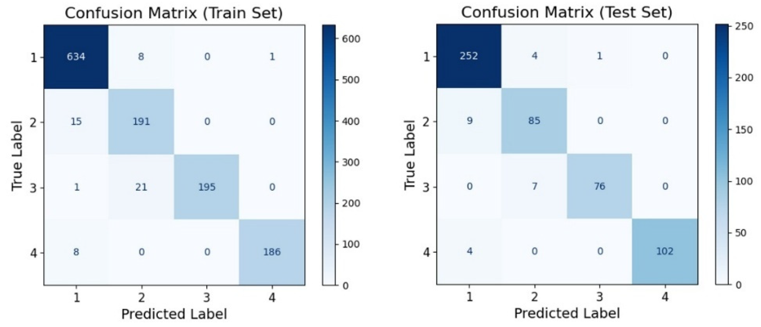
Next, the 9-dimensional feature dataset without composite multiscale entropy features is used as the input of the random forest model and compared with the experimental results of the 11-dimensional feature dataset containing composite multiscale entropy features to verify the effectiveness of the composite multiscale entropy features. The experimental results are shown in the confusion matrix in Figure 6, The training set accuracy of the 9-dimensional feature dataset is only 95.71%, and the test set accuracy is 95.37%. By comparing the experimental results of the 9-dimensional and 11-dimensional feature datasets, the validity and significant contribution of the composite multiscale entropy feature to the discriminative power of the measurement model can be proved initially.

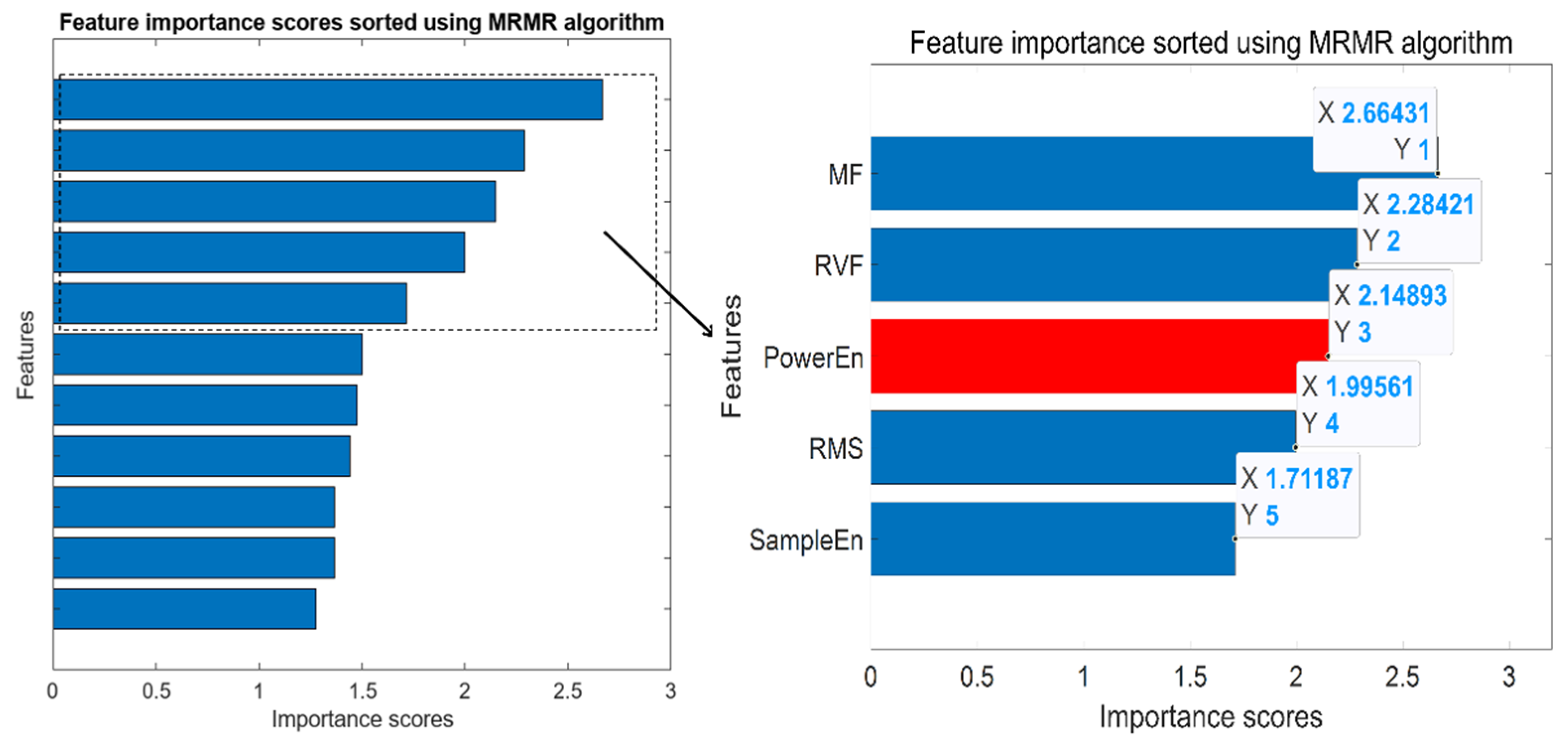
The importance of 11-dimensional features is ranked using the MRMR algorithm. After obtaining the feature importance ranking, we sequentially select features from high to low, from one dimension to multidimensional, using the Random Forest algorithm for classification training experiments. The experiments show that the highest accuracy of 98.15% is achieved when the features are selected up to 5 dimensions, whereas the selection of features in 6 dimensions and above leads to a gradual decrease in the accuracy due to feature redundancy. Thus, the iteration is stopped when the subset size reaches five features, which serves as the preset termination condition, and these top five ranked features are taken as inputs to the final algorithm, and the results are shown in Figure 7. We can see that the top five features are the time-domain feature margin factor (MF), root-mean-square (RMS), the frequency-domain feature standard frequency difference (RVF), and our newly proposed composite multiscale power spectral entropy (PowerEn) and composite multiscale sample entropy (SampleEn). This result not only further proves the high efficiency of our newly proposed composite multiscale power spectral entropy and composite multiscale sample entropy, but also demonstrates the ability of the MRMR algorithm to identify a compact yet highly discriminative feature set that is optimal for measurement.

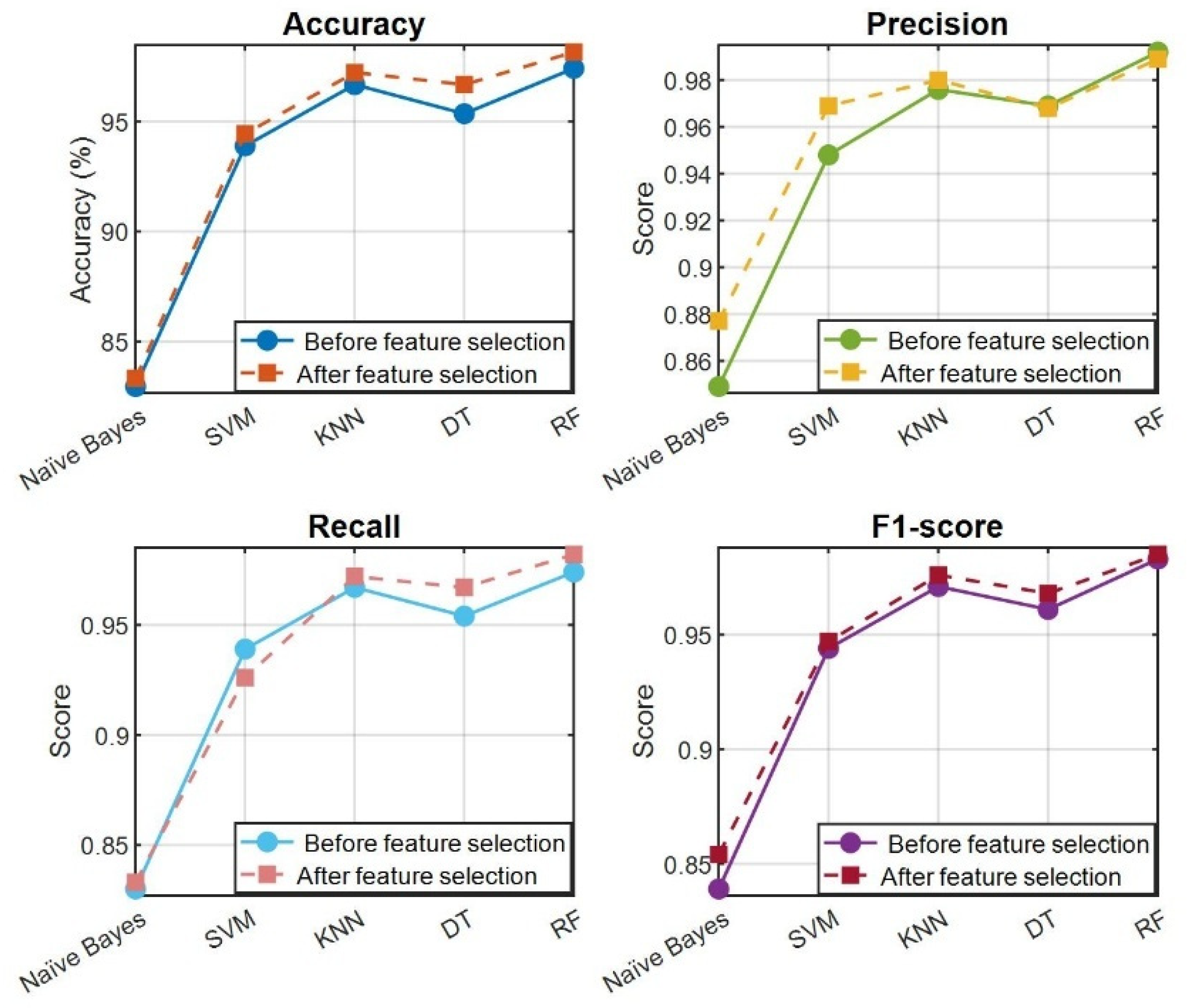
In order to verify the stability and generalizability of the feature selection results, a 5-dimensional feature dataset is used as the input of the other four algorithms in this paper, and the results are shown in

Table 8. Test results after feature selection.

Number	Algorithm	Accuracy	Precision	Recall	F1-Score
1	Naïve Bayes	83.33%	0.877	0.833	0.854
2	SVM	94.44%	0.916	0.887	0.884
3	KNN	97.22%	0.980	0.972	0.976
4	DT	96.67%	0.968	0.967	0.968
5	RF	98.15%	0.989	0.982	0.985

and Figure 8. The experimental results demonstrate that the performance metrics of all five algorithms have improved to varying degrees when using the MRMR-selected subset, which further confirms the stability, portability and effectiveness of the proposed feature selection method across different classification paradigms.

After completing feature selection using the MRMR algorithm, this study employs the random search algorithm to optimize the hyperparameters of the random forest. The initial parameter ranges and the corresponding optimal values are presented in

Table 9. Parameter ranges and optimal values.

Parameter Name	Parameter Range	Optimal Value
n_estimators	10~200	94
max_depths	1~30	13
max_features	1~20	2
min_samples_split	1~20	3
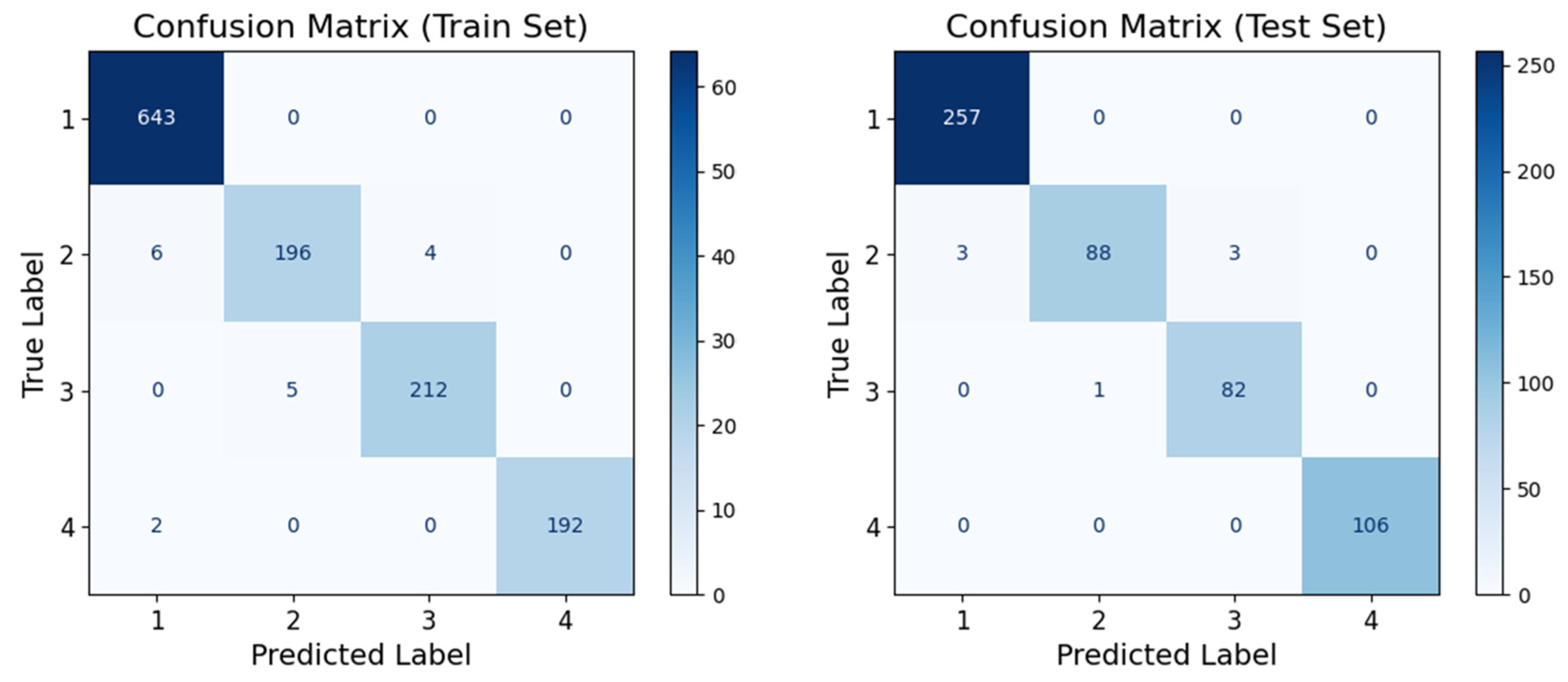
min_samples_leaf	1~20	2

. The confusion matrix for the training and testing results based on the optimal parameter combination is shown in Figure 9. The parameter boundaries used in the random search (Table 9) were selected based on empirical guidelines, prior literature, and considerations of dataset size and feature dimensionality. The chosen ranges strike a balance between model flexibility and computational cost, while avoiding overfitting given the small sample size, and the performance metrics of the optimized model are summarized in

Table 10. Comparison of detection time and accuracy before and after optimization.

Performance Indicators	Before Parameter Optimization	After Parameter Optimization
Accuracy	98.15%	98.70%
Precision	0.989	1
Recall	0.973	0.986
F1-score	0.986	0.993
Time	7 ms	10 ms

. The results indicate that except for a slight increase in computation time by 3 ms—caused by the optimized parameters being generally larger than the default values—all performance metrics have improved, culminating in a final model accuracy of 98.70%. This represents a 0.55% improvement over the unoptimized version. Although the absolute accuracy gain may appear modest, the optimization consistently enhanced other critical metrics such as precision (reaching 1.000), recall, and F1-score (0.993), which are paramount for minimizing false alarms and missed detections in safety-critical measurement applications. Considering that typical arc fault detection response time requirements in electrical systems are on the order of tens to hundreds of milliseconds, this additional latency remains well within acceptable limits and does not compromise the practical utility of the measurement system. Therefore, the hyperparameter optimization is justified as it yields a more reliable and robust classifier without incurring prohibitive computational costs. These experimental findings demonstrate that the random search algorithm can effectively optimize the hyperparameters of the random forest, thereby enhancing model performance and enabling more efficient arc fault detection.

5. Conclusions

This paper proposes an interpretable and robust AC series arc fault detection framework integrating composite multiscale entropy (CMSE) features, MRMR-based feature selection, and a random search-optimized random forest classifier. The results demonstrate that multiscale entropy features effectively capture nonlinear waveform distortions induced by arc faults, while redundancy-aware feature selection enhances discriminability and reduces model complexity. The optimized model achieves a final detection accuracy of 98.70%, confirming the effectiveness of the integrated feature–selection–classification strategy.

Although the present validation is conducted on a 400 Hz experimental platform representative of aerospace and marine power systems, the proposed framework is not inherently frequency-dependent. Since the entropy-based complexity measures and structural feature selection operate on normalized quasi-periodic signal characteristics rather than absolute frequency values, the method can be extended to conventional 50/60 Hz residential and industrial AC systems with appropriate retraining and parameter adaptation, demonstrating promising cross-frequency scalability.

Nevertheless, this study remains limited to offline laboratory validation using 1800 samples across nine load types. Future work will focus on real-time embedded implementation, validation under more complex and interference-prone environments, and the incorporation of transfer learning strategies to enhance cross-system adaptability and large-scale deployment feasibility.