Layered Multi-Objective Optimization of Permanent Magnet Synchronous Linear Motor Considering Thrust Ripple Suppression

Abstract

In this study, a layered multi-objective optimization design method is proposed for a segmented skewed pole permanent magnet synchronous linear motor (PMSLM), considering thrust ripple suppression. Based on a 2-D analytical model, the effects of end force, cogging force, and winding asymmetry force on thrust ripple in PMSLM are analyzed, and the correctness is verified using finite element analysis and experiments. On this basis, a layered multi-objective optimization method is proposed. The whole optimization is divided into three layers. Metamodels of optimal prognosis are established to optimize the structural parameters in a layered manner, achieving a compromise between reducing thrust ripple and increasing average thrust. The effectiveness of the layered multi-objective optimization method is verified through simulation and prototype experiments. The layered structure aims to improve efficiency while ensuring computational accuracy.

1. Introduction

Electric machines continue to attract strong research and development interest due to the ongoing electrification of industry and transportation, as well as the demand for higher efficiency, reliability, and accuracy in motion systems. Recent studies have highlighted continuous advances in mathematical modeling and experimental validation for induction motor dynamics, emerging trends and developments in permanent magnet motor technologies, and fault detection and diagnostic methodologies for synchronous motors, reflecting broad and active research directions in the motor community [1,2,3]. In parallel, high-precision direct-drive applications have made thrust ripple suppression and computationally efficient design optimization of permanent magnet linear machines increasingly important, motivating mechanism-oriented modeling and surrogate-assisted multi-objective optimization frameworks.

Permanent magnet synchronous linear motors (PMSLMs) are commonly used in high-precision computer numerical control machines, laser cutting machines, etc., eliminating intermediate mechanical parts and offering the advantages of high precision, high efficiency, and strong reliability [4,5]. However, the end effect force, cogging force, and winding asymmetry effect force in PMSLMs can cause thrust ripple, resulting in speed fluctuations, increased servo control burden, degraded motion stability and dynamic response, and consequently reduced positioning and control precision. In [6], an auxiliary tooth is designed in which the end force was greatly weakened by changing its height and width. The influence of different winding forms on the cogging force is studied [7]. In [8], the researchers pointed out that the existence of winding asymmetry caused magnetic coupling between the d-axis and the q-axis, which directly caused the thrust ripple of the motor. Therefore, to achieve the best performance of the PMSLM, motor design optimization is a crucial step and always deserves attention, with both single-objective and multi-objective optimization design methods being proposed and realized.

For single-objective optimization, it can be achieved by optimizing the structural parameters of the PMSLM. However, motor design optimization is a high-dimensional problem with strong coupling of multiple physical fields and nonlinearity, where optimization objectives often conflict with each other under constraints. Traditional single-objective optimization methods cannot meet the requirements [9,10]. For this reason, multi-objective optimization methods are used to achieve an optimal balance among different performance objectives.

For multi-objective optimization, various optimization algorithms have been widely used to enhance the overall performance of electrical machines [11]. Although different optimization algorithms employ different search mechanisms, they share a common goal: efficiently exploring the trade-offs among multiple competing objectives under constraints, such as reducing mass while increasing average thrust or reducing iron loss while suppressing thrust ripple [12,13,14,15]. For PMSLMs serving as precision direct-drive actuators, improving the average thrust and suppressing thrust ripple typically constitute one of the most fundamental trade-off pairs in multi-objective optimization. This trade-off directly affects industrial performance: reducing thrust ripple improves positioning accuracy, while increasing average thrust improves energy efficiency. However, it is computationally intensive when too many motor parameters are involved in the optimization. This leads to a large number of iterations and convergence difficulties, which decrease the efficiency of the optimization process. Therefore, layered multi-objective optimization methods are proposed to meet optimization demands and achieve a balanced design [16,17,18,19].

In the current research on layered optimization, design variables are typically screened and stratified according to sensitivity ranking [20,21,22,23], which is effective for variable selection. However, from the perspective of PMSLM thrust ripple mechanisms, sensitivity-based stratification does not explicitly reflect the physical sources of thrust ripple. As a result, variables related to the end-effect force, cogging force, and winding asymmetry-induced force can be placed in the same layer, which may retain cross-mechanism coupling and weaken the interpretability and targeted effectiveness of the optimization process. Nevertheless, layered optimization remains a practical way to handle high-dimensional motor design problems, especially when combined with appropriate modeling and search strategies.

Research indicates that optimizing parameters across different design layers can address the optimization problems of motors with a large number of design parameters. However, optimization algorithms based on offline data-driven approaches cannot actively generate new samples during the optimization process. Therefore, in order to reduce computational costs, surrogate models are widely applied in optimization algorithms. For example, neural network models are used to predict the performance parameters of motors [24,25]. The response surface method involves a central composite design to optimize the single-sided, flat-tooth, unequal-width permanent magnet synchronous linear motor [26]. Kriging models are used in the three-level optimization strategy for the multi-objective optimization design of interior permanent magnet synchronous motors (IPMSMs) to analyze IPMSMs in order to achieve lower torque ripple and higher power output [22]. A modified particle swarm optimization algorithm with an embedded extreme learning machine is used to improve accuracy and efficiency for global optimization of a micro-joint motor with multiple modes [27]. Although online data-driven optimization greatly improves the efficiency of multi-objective optimization for motors, the accuracy of the surrogate model is limited by the number of selected structural parameters and is also closely related to the choice of surrogate model type [28]. If a single surrogate model is fixed in advance, its adaptability to different problem characteristics is limited, which can readily increase prediction errors. Therefore, it is crucial to reconcile the trade-off between high model accuracy and high optimization efficiency.

In order to solve these issues, a layered multi-objective optimization design method for a segmented skewed pole PMSLM, considering thrust ripple suppression, is proposed in this study based on a 2-D analytical model. The proposed layering is guided by the thrust ripple source mechanisms: the design parameters are classified into different layers according to their dominant influence on the end effect force, cogging force, winding asymmetry effect force, and skew design, thereby weakening coupling and improving physical interpretability. In addition, the Metamodel of Optimal Prognosis (MOP) is employed to evaluate and compare the prognosis quality of multiple candidate surrogate models, and the best-performing surrogate is automatically selected for the subsequent multi-objective optimization. This improves surrogate reliability under a limited sample budget. Overall, the proposed method partially decouples the structural parameters from the performance indicators, which is important for maintaining surrogate accuracy and improving computational efficiency. This study is organized as follows. In Section 2, the motor topology is introduced, and the effect of the three forces on thrust ripple is analyzed. Then, a layered multi-objective optimization method is proposed in Section 3. Section 4 analyzes the performance of the motor after optimization. In Section 5, the prototype is manufactured, and the experimental platform is set up. Finally, Section 6 concludes this study.

2. Thrust Ripple Analysis of PMSLM

The original design of the segmented skewed pole PMSLM is a three-phase, 12 s/14 p, Y-connected motor as shown in Figure 1. Compared with the continuous skew pole, the segmented skewed pole is equally effective in reducing the thrust ripple.

2.1. End Force Analysis

The end force F_end is caused by primary core disconnection and is the sum of left end force F_l and right end force F_r. The relationship between F_l and F_r can be expressed as

$${\left.F_{\mathrm{l}}\right|}_{x=x^{\prime }}=-{\left.F_{\mathrm{r}}\right|}_{x=-\left(x^{\prime }+\delta \right)},\delta =k\tau -L_{\mathrm{s}},$$

(1)

where x is the primary core displacement, k is an integer, τ is the pole pitch of the permanent magnet, L_s is the primary core length. τ = 10 mm and L_s = kτ = 150 mm are the first set.

In (1), F_r can be expressed using a Fourier series as follows:

$$F_{\mathrm{r}}=F_0+{\displaystyle \sum _{n=1}^n}\left(f_{\mathrm{s}n}\sin {\displaystyle \frac{2n\mathrm{\pi }}{\tau }}x+f_{\mathrm{c}n}\cos {\displaystyle \frac{2n\mathrm{\pi }}{\tau }}x\right)$$

(2)

where F₀ is the DC component, f_sn is the amplitude of the nth harmonic sine series, and f_cn is the amplitude of the nth harmonic cosine series, n = 1, 2, 3….

In (1), F_l can be expressed using a Fourier series as follows:

$$F_{\mathrm{l}}=-F_0+{\displaystyle \sum _{n=1}^n}\left(f_{\mathrm{s}n}\sin {\displaystyle \frac{2n\mathrm{\pi }}{\tau }}\left(x+\delta \right)-f_{\mathrm{c}n}\cos {\displaystyle \frac{2n\mathrm{\pi }}{\tau }}\left(x+\delta \right)\right)$$

(3)

Therefore, F_end can be expressed as the sum of Equations (2) and (3):

$$F_{\mathrm{end}}=F_{\mathrm{r}}+F_{\mathrm{l}}={\displaystyle \sum _{n=1}^{\infty }}2\left(f_{\mathrm{s}n}\cos {\displaystyle \frac{n\mathrm{\pi }}{\tau }}\delta +f_{\mathrm{c}n}\sin {\displaystyle \frac{n\mathrm{\pi }}{\tau }}\delta \right)\sin {\displaystyle \frac{2n\mathrm{\pi }}{\tau }}\left(x+{\displaystyle \frac{\delta }{2}}\right)$$

(4)

From (4), it can be seen that a DC component is not included in F_end. F_end varies in magnitude at different positions, being a periodic function of τ, and is related to L_s. F_end can be reduced by decreasing the fundamental wave. A fourth-order Fourier series is used to perform nonlinear regression on F_r and F_l, respectively:

$$\begin{array}{c}{F}_{\mathrm{r}}=12.383+8.4724\sin \left({\displaystyle \frac{2\mathrm{\pi }}{10}}x\right)+0.8003\sin \left({\displaystyle \frac{4\mathrm{\pi }}{10}}x\right)+0.0807\sin \left({\displaystyle \frac{6\mathrm{\pi }}{10}}x\right)+0.0865\sin \left({\displaystyle \frac{8\mathrm{\pi }}{10}}x\right)++0.444\cos \left({\displaystyle \frac{2\mathrm{\pi }}{10}}x\right)+\\ +0.8751\cos \left({\displaystyle \frac{4\mathrm{\pi }}{10}}x\right)+0.2537\cos \left({\displaystyle \frac{6\mathrm{\pi }}{10}}x\right)+0.2491\cos \left({\displaystyle \frac{8\mathrm{\pi }}{10}}x\right)\end{array}$$

(5)

$$\begin{array}{c}{F}_{\mathrm{l}}=-12.383+8.4724\sin \left({\displaystyle \frac{2\mathrm{\pi }}{10}}x\right)+0.8003\sin \left({\displaystyle \frac{4\mathrm{\pi }}{10}}x\right)+0.0807\sin \left({\displaystyle \frac{6\mathrm{\pi }}{10}}x\right)+0.0865\sin \left({\displaystyle \frac{8\mathrm{\pi }}{10}}x\right)-0.444\cos \left({\displaystyle \frac{2\mathrm{\pi }}{10}}x\right)\\ -0.8751\cos \left({\displaystyle \frac{4\mathrm{\pi }}{10}}x\right)-0.2537\cos \left({\displaystyle \frac{6\mathrm{\pi }}{10}}x\right)-0.2491\cos \left({\displaystyle \frac{8\mathrm{\pi }}{10}}x\right)\end{array}$$

(6)

From (5) and (6), it can be seen that f_s1 = 8.4724 N, f_c1 = 0.444 N, so the optimal fundamental wave length δ_opt can be expressed as

$${\delta }_{\mathrm{opt}}={\displaystyle \frac{\tau }{\mathrm{\pi }}}\arctan \left(-{\displaystyle \frac{f_{\mathrm{s}1}}{f_{\mathrm{c}1}}}\right)={\displaystyle \frac{10}{\mathrm{\pi }}}\mathrm{a}\mathrm{r}\mathrm{c}\mathrm{t}\mathrm{a}\mathrm{n}\left({\displaystyle \frac{8.4724}{0.444}}\right)=4.833\approx 5$$

(7)

Considering the symmetry of the PMSLM windings, take δ_opt = 5 mm; thus, the optimized primary core length L′_s = 15τ − δ_opt = 145 mm. With this optimized δ_opt, it can be seen that compared with F_end, F′_end does not contain the odd terms of the sine series and the even terms of the cosine series, leaving only the high-order harmonics with a period at 2τ and above. Therefore, by optimizing δ, and thereby optimizing L_s, the harmonic content of the end force can be significantly reduced.

2.2. Cogging Force Analysis

The cogging force of the PMSLM is affected by slot numbers, which in turn are related to the winding forms. When single-layer winding or double-layer overlapping integral pitch winding is used, the actual slot number N_s′ of the linear motor is consistent with the effective slot number N_s, but when double-layer overlapping short pitch winding is used, it is one more than N_s.

The cogging force f_s1 produced by a single slot fluctuates periodically with pole pitch and contains numerous harmonics. The Fourier series expansion of f_s1 can be expressed as

$$f_{s1}={\displaystyle \sum _{n=1}^{\infty }}{F}_n\cos \left({\displaystyle \frac{2n\mathrm{\pi }}{\tau }}x+{\displaystyle \frac{{\phi }_n}{180°}}\mathrm{\pi }\right),n=\mathrm{1,2},3,\dots$$

(8)

The Fourier series expansion of f_s1 produced by different slots is the same. Due to the different initial positions of each slot, the initial phase is different. Ignoring the interaction between the slots, the cogging force f_s produced by all the slots can be regarded as the superposition of multiple f_s1.

The pole number of the motor is N_p, the distance between the slots is N_pτ/N_s. In order to simplify the analysis, the slots are rearranged in two cases. First, if N_s and N_p are prime, the slots are evenly distributed, and the angular position difference between the slots is 2π/N_s. Second, if N_s and N_p have the greatest common divisor l, then the slots are evenly distributed l times, and the angular position difference between the slots is 2lπ/N_s.

When N_s’ is equal to N_s, the f_s can be expressed as

$$f_{\mathrm{s}}={\sum }_{i=1}^{N_{\mathrm{s}}}{\sum }_{n=1}^{\infty }{F}_n\left[\cos {\displaystyle \frac{2n\mathrm{\pi }}{\tau }}\left(x+{\displaystyle \frac{(i-1)\tau l}{N_{\mathrm{s}}}}\right)+{\displaystyle \frac{{\phi }_n}{180°}}\mathrm{\pi }\right]=N_{\mathrm{s}}{\sum }_{n=1}^{\infty }{F}_{n{N}_{\mathrm{s}}/l}\cos \left({\displaystyle \frac{2n{N}_{\mathrm{s}}\mathrm{\pi }}{l\tau }}x+{\displaystyle \frac{{\phi }_{\frac{n{N}_{\mathrm{s}}}{l}}}{180°}}\mathrm{\pi }\right)$$

(9)

It can be seen from (9) that the f_s′ is composed of f_s and f_s1, which contains not only the N_s/l order harmonic, but also numerous low-order harmonics.

The winding form used in this paper is shown in Figure 1, where N_s′ is equal to N_s, resulting in low harmonic content. Consequently, the cogging force of the motor is f_s″.

The finite element analysis (FEA) verification of the cogging force analysis is shown in Figure 2. It can be seen from Figure 2a that the peak-to-peak value of f_s1 is large because it contains numerous harmonics. The peak-to-peak value of f_s′ is very close to that of a single slot, and the peak-to-peak value of f_s″ is relatively small. It can be seen from Figure 2b that f_s1 is mainly composed of first harmonic, second harmonic, and third harmonic; f_s′ is mainly composed of first harmonic, second harmonic, third harmonic, and sixth harmonic; and the first harmonic amplitude of the f_s″ is smaller than the first two cases.

2.3. Winding Asymmetry Force Analysis

Primary core disconnection also causes the winding to be asymmetrical. Under three-phase sinusoidal current excitation, additional voltage components are generated, which can be expressed as

$$\left\{\begin{array}{c}{e}_{\mathrm{SA}1}={\displaystyle \frac{\mathrm{d}{\psi }_{\mathrm{SA}}}{\mathrm{d}t}}={\displaystyle \frac{\mathrm{d}\left(0\cdot i_{\mathrm{A}}+M_{\mathrm{k}}{i}_{\mathrm{B}}+0\cdot i_{\mathrm{C}}\right)}{\mathrm{d}t}}={\displaystyle \frac{\mathrm{d}\left(M_{\mathrm{k}}{i}_{\mathrm{B}}\right)}{\mathrm{d}t}}\\ e_{\mathrm{SB}1}={\displaystyle \frac{\mathrm{d}{\psi }_{\mathrm{SB}}}{\mathrm{d}t}}={\displaystyle \frac{\mathrm{d}\left(M_{\mathrm{k}}{i}_{\mathrm{A}}+0\cdot i_{\mathrm{B}}+0\cdot i_{\mathrm{C}}\right)}{\mathrm{d}t}}={\displaystyle \frac{\mathrm{d}\left(M_{\mathrm{k}}{i}_{\mathrm{A}}\right)}{\mathrm{d}t}}\\ e_{\mathrm{SC}1}={\displaystyle \frac{\mathrm{d}{\psi }_{\mathrm{SC}}}{\mathrm{d}t}}={\displaystyle \frac{\mathrm{d}\left[{\psi }_k\cos (\frac{\mathrm{\pi }}{\tau }x+\frac{2\mathrm{\pi }}{3})+0\cdot i_{\mathrm{A}}+0\cdot i_{\mathrm{B}}+L_{\mathrm{k}}{i}_{\mathrm{C}}\right]}{\mathrm{d}t}}\\ ={\displaystyle \frac{\mathrm{d}\left[{\psi }_k\cos (\frac{\mathrm{\pi }}{\tau }x+\frac{2\mathrm{\pi }}{3})+L_{\mathrm{k}}{i}_{\mathrm{C}}\right]}{\mathrm{d}t}}\end{array}\right.$$

(10)

where e_SA1, e_SB1, e_SC1 are the voltage component generated by winding asymmetry; Ψ_SA, Ψ_SB, Ψ_SC are the flux linkage component generated by winding asymmetry; i_A, i_B, i_C are the three-phase sinusoidal current; L_k is the DC component difference in self-inductance between phase C, phase A, and phase B; M_k is the DC component difference in mutual inductance between phase C, phase A, and phase B; and Ψ_k is the DC component difference in flux linkage between the phase C, phase A, and phase B.

When the motor is running at uniform speed, the thrust f_em can be expressed as

$$f_{\mathrm{em}}={\displaystyle \frac{m{e}_{\mathrm{A}}{i}_{\mathrm{A}}}{v}}$$

(11)

where m is the number of phases, e_A is the no-load back electromotive force (EMF) of phase A.

It can be seen from (11) that the winding asymmetric force f_wa can be expressed as

$$f_{\mathrm{wa}}={\displaystyle \frac{\left(e_{\mathrm{SA}1}{i}_{\mathrm{A}}+e_{\mathrm{SB}1}{i}_{\mathrm{B}}+e_{\mathrm{SC}1}{i}_{\mathrm{C}}\right)}{v}}={\displaystyle \frac{\mathrm{\pi }{\psi }_{\mathrm{k}}{I}_0}{2\tau }}+{\displaystyle \frac{\mathrm{\pi }{\psi }_{\mathrm{k}}{I}_0}{2\tau }}\cos \left({\displaystyle \frac{2\mathrm{\pi }}{\tau }}x-{\displaystyle \frac{2\mathrm{\pi }}{3}}\right)-{\displaystyle \frac{\mathrm{\pi }{L}_{\mathrm{k}}{I}_0^2}{2\tau }}\sin \left({\displaystyle \frac{2\mathrm{\pi }}{\tau }}x-{\displaystyle \frac{2\mathrm{\pi }}{3}}\right)-{\displaystyle \frac{\mathrm{\pi }{M}_{\mathrm{k}}{I}_0^2}{\tau }}\sin \left({\displaystyle \frac{2\mathrm{\pi }}{\tau }}x+{\displaystyle \frac{\mathrm{\pi }}{3}}\right)$$

(12)

It can be seen from Equation (12) that f_wa is related to Ψ_k, L_k and M_k, all of which are related to the number of turns in the three-phase winding.

3. Layered Multi-Objective Optimization of PMSLM

3.1. Layered Multi-Objective Optimization Principle Analysis

To further balance the relationship between thrust ripple and average thrust of the PMSLM and enhance its overall performance, multi-objective optimization is conducted on it. Considering the large number of structural parameters, slow convergence, and the large amount of computation involved, a method of optimizing the variables in layers is adopted to improve the efficiency of the optimization process.

3.1.1. Objective Function

The average thrust and thrust ripple are taken as optimization objectives in this study. The numerical scale of the average thrust and the thrust ripple are significantly different, so the normalization is carried out.

The objective function can be expressed as

$$\left\{\begin{array}{c}{f}_{\mathrm{m}\mathrm{i}\mathrm{n}}{=\lambda }_1{\displaystyle \frac{F_{avg}\left(x_i\right)}{F_{avg}^{°}\left(x_i\right)}}+{\lambda }_2{\displaystyle \frac{R_{ripple}^{°}\left(x_i\right)}{R_{ripple}\left(x_i\right)}}\\ {\lambda }_1={\lambda }_2=0.5\\ {\lambda }_1+{\lambda }_2=1\end{array}\right.$$

(13)

where F°_avg(x_i) is the optimized average thrust, R°_ripple(x_i) is the optimized thrust ripple, F_avg(x_i) is the average thrust before optimization, R_ripple(x_i) is the thrust ripple before optimization, and λ₁ and λ₂ are weight coefficients. According to the objective function f_min(x_i), the optimized initial value for average thrust F_avg(x_i) is placed on the numerator, while the optimized initial value for thrust ripple R_ripple(x_i) is placed on the denominator. As the optimized average thrust F°_avg(x_i) increases, F_avg(x_i)/F°_avg(x_i) decreases. Meanwhile, as the optimized thrust ripple R°_ripple(x_i) decreases, R°_ripple(x_i)/R_ripple(x_i) will also decrease. Therefore, according to the requirements of motor design, it is necessary to seek the minimum value of the multi-objective optimization function f_min(x_i). Due to the equal importance of the requirements for average thrust and thrust ripple, the weight coefficients λ₁ and λ₂ in the objective function are both set to 0.5, satisfying the relationship of λ₁ + λ₂ = 1.

3.1.2. Optimization Variable

The optimal variables of the PMSLM are listed in

Table 1. Optimal variables of PMSLM.

Items	Symbol
Permanent magnet width	τm
Permanent magnet height	hm
Slot width	ws
Slot height	hs
End width	we
Number of turns in phase A	tA
Number of turns in phase B	tB
Number of turns in phase C	tC
Number of skew pole segments	N
Skew pole angle	θ

.

3.1.3. Constraint Condition

The structural parameters of the motor are constrained by conditions such as the working scene, mechanical size and safe operation, and should be within a reasonable range. Value ranges of 10 optimization parameters can be expressed as

$$\begin{array}{cc}8.2 \mathrm{mm}\le {\tau }_{\mathrm{m}}\le 9.3 \mathrm{mm}& 1.5 \mathrm{mm}\le h_{\mathrm{m}}\le 2.5 \mathrm{mm}\\ 5.3 \mathrm{mm}\le w_{\mathrm{s}}\le 6.3 \mathrm{mm}& 10.5 \mathrm{mm}\le h_{\mathrm{s}}\le 11.5 \mathrm{mm}\\ 2.435 \mathrm{mm}\le w_{\mathrm{e}}\le 3.435 \mathrm{mm}& 67\le t_{\mathrm{A}}\le 71\\ 67\le t_{\mathrm{B}}\le 71& 67\le t_{\mathrm{C}}\le 71\\ 3\le N\le 6& 30°\le \theta \le 75°\end{array}$$

(14)

3.1.4. Mechanism of Layered Multi-Objective Optimization Method

Based on the analysis of the three forces causing thrust ripple, τ_m, h_m, w_s, h_s, and w_e are parameters related to the cogging force and the end force of the PMSLM. t_A, t_B, and t_C affect the winding asymmetry effect force of the PMSLM, while N and θ themselves are means of reducing the thrust ripple of the PMSLM. Therefore, according to these considerations, the parameters are divided into three layers for optimization. It can be seen from Figure 3 that this method consists of five steps.

Step 1: Determine the objective function, specify the optimization variables, and set the corresponding constraints.

Step 2: According to the layering rules, the motor structure parameters are divided into three layers.

Step 3: The first layer optimization. The structural parameters of the first layer are about the end and the tooth groove. An orthogonal table is established using the Taguchi method to calculate the signal-to-noise ratio (SNR) of thrust ripple in each group. The most sensitive parameters are identified through analysis of variance (ANOVA). The advanced Latin hypercube (ALH) method is used to sample, and the metamodels of optimal prognosis (MOPs) are constructed using calculated average thrust and thrust ripple. The multi-objective PSO is finally used to find the Pareto solution set. The selected optimal values are then fixed as the final first layer outcomes, and they serve as fixed inputs for the subsequent second layer optimization.

Step 4: The second layer optimization. The second layer structure parameter is the number of winding turns. The process is similar to the first layer optimization; the MOPs are established, and the multi-objective PSO is used to find the Pareto solution set. The selected optimal t_A, t_B, and t_C are then fixed as the final second layer result.

Step 5: The third layer optimization. The structural parameters of the third layer are segmented skew pole structure parameters. The orthogonal table is established by the multi-objective Taguchi method, and the thrust ripple and average thrust of each group are substituted into the objective function to solve and compare, and the final structural parameters are determined.

3.2. The First Layer Optimization Considering Sensitivity

3.2.1. Parameter Sensitivity Analysis

The first layer has many structural parameters, which affect the accuracy and efficiency of the model, so the sensitivity analysis of the parameters should be carried out. To improve computational efficiency, the L25 Taguchi method is used to establish the sample database and calculate the corresponding thrust ripples instead of the traversal method. Detailed parameters and their levels are shown in

Table 2. Parameters and their levels.

Items	Level 1	Level 2	Level 3	Level 4	Level 5
ws (mm)	5.3	5.55	5.8	6.05	6.3
hs (mm)	10.5	10.75	11	11.25	11.5
hm (mm)	1.5	1.75	2	2.25	2.5
τm (mm)	8.2	8.45	8.7	9.05	9.3
we (mm)	2.435	2.685	2.935	3.185	3.435

.

The SNR is used to quantitatively assess the extent to which noise factors affect motor characteristics. In the multi-objective optimization of a motor, the thrust ripple is taken as the optimization objective, and the SN_i has the characteristics of low expectation. It can be expressed as

$$S{N}_i=-10\log \left({\displaystyle \frac{1}{n}}{X}_i^2\right)$$

(15)

where i corresponds to group i, n is the number of samples, and X_i is the thrust ripple corresponding to group i.

The SNR of thrust ripples of each group is calculated, and then the sensitivity analysis is performed by ANOVA. The sensitivity S_X of parameter x can be expressed as

$$S_{\mathrm{x}}={\displaystyle \frac{1}{t}}{\displaystyle \sum _{j=1}^t}{\left(M_{\mathrm{x}j}\left(S{N}_i\right)-M_{\mathrm{x}}\left(S{N}_i\right)\right)}^2$$

(16)

where t is the number of levels of x, M_x(SN_i) is the average of SN_i, M_xj(SN_i) is the average of SN_i when the number of levels of x is j.

M_x(SN_i), M_xj(SN_i) can be expressed as

$$\left\{\begin{array}{c}{M}_{\mathrm{x}}(S{N}_i)={\displaystyle \frac{1}{n}}{\displaystyle \sum _{i=1}^n}S{N}_i\\ M_{\mathrm{x}j}\left(S{N}_i\right)={\displaystyle \frac{1}{m}}{\displaystyle \sum _{i=1}^m}S{N}_i\end{array}\right.$$

(17)

After calculation, the sensitivity of the first layer parameters is shown in Figure 4. Figure 4a shows the SNR of thrust ripple, where the greater the dispersion of the points, the higher the sensitivity of the parameter to thrust ripple. It can be seen that the three parameters with the highest sensitivity are the w_e, h_m, and w_s. In order to more intuitively represent the degree of influence of the first layer parameters on thrust ripple, the sensitivity analysis results are given as shown in Figure 4b. From the figure, it can be seen that the sensitivity analysis results are consistent with the SNR results at each level.

3.2.2. Establishment of the MOPs

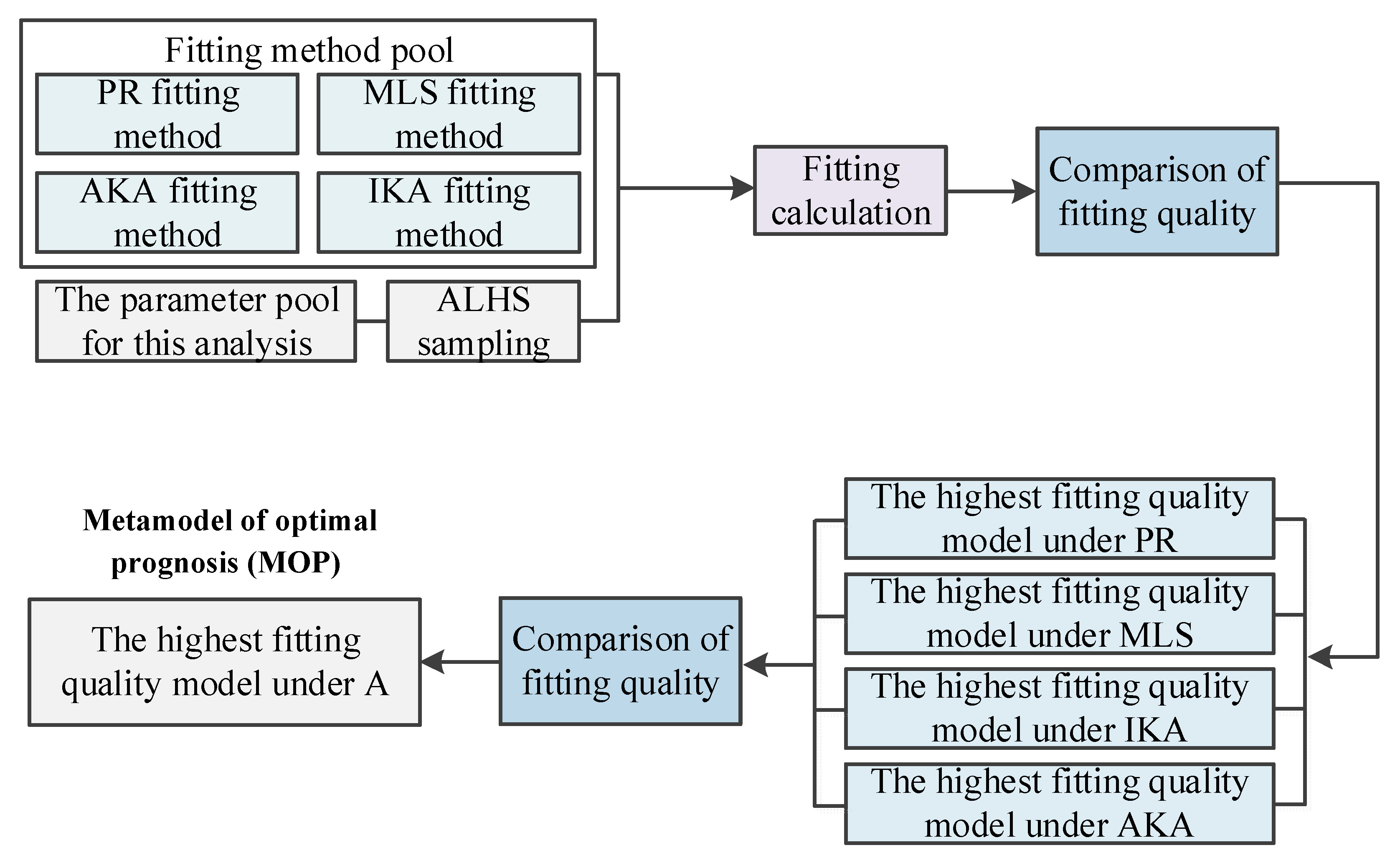
At present, the commonly used methods for establishing surrogate models include Polynomial Regression (PR), Gaussian Process Regression (GPR), and Moving Least Squares (MLS). In GPR, the commonly used methods include Anisotropic Kriging Approximation (AKA) and Isotropic Kriging Approximation (IKA). The accuracy of the surrogate model is the basis for optimizing the motor. Based on the above method of establishing the surrogate model, the MOP has been proposed in recent years. The generation process of the MOP is shown in Figure 5. Firstly, the fitting models under the four fitting methods are established, and then the fitting quality is compared to select the best fitting model, and finally, the model is determined as the MOP. The MOP does not create a new fitting method. On the basis of the original fitting method, the screening mechanism is introduced to find the best surrogate model.

The ALH method is used for sampling. This method can not only ensure the global sample, but also reduce the number of samples and ensure the computational efficiency of the surrogate model. 120 sample points were collected. The samples are substituted into the FEA, corresponding thrust ripple and average thrust are obtained, and MOPs are established based on these data.

To evaluate the quality of MOP, the model prediction accuracy coefficient is defined, which can be expressed as

$${\delta }_{\mathrm{P}}=1-{\displaystyle \frac{E_{\mathrm{P}}}{E_{\mathrm{T}}}}$$

(18)

where E_P is the sum of squares of the prediction error of the MOP, and E_T is the sum of squares of the difference between a sample and the mean of all samples.

The E_P can be expressed as

$$E_{\mathrm{P}}={{\displaystyle \sum _{i=1}^N}\left(\widehat{g_i}-g_i\right)}^2$$

(19)

where $\widehat{g_i}$ is the fitting results based on MOP of group i, and $g_i$ is the actual result for group i.

The E_T can be expressed as

$$E_{\mathrm{T}}={{\displaystyle \sum _{i=1}^N}\left(g_i-u_{\mathrm{g}}\right)}^2$$

(20)

where u_g is the average of the actual results.

The prediction accuracy of the MOP is the highest when δ_P equals 1. Combined with practice, to improve the calculation accuracy of the MOP, the datum δ_PS is set to 95%, and the error between the fitting model and the actual model does not exceed 5% of the actual model.

In the first layer optimization, MOPs of average thrust and thrust ripple are shown in Figure 6 and Figure 7. It can be seen from Figure 6 and Figure 7 that the prediction accuracy coefficient of MOPs of average thrust is 99%, and the prediction accuracy coefficient of MOPs of thrust ripple is 91%.

3.2.3. Multi-Objective Optimization Based on PSO

The MOPs are optimized using a multi-objective PSO. The detailed parameter settings of the PSO are summarized in

Table 3. PSO parameter settings.

Item	Value
Swarm size	40
Max iterations	120
Archive size	150
Grid divisions	12
Inertia weight	Adaptive
Acceleration coefficients	2

. Optimization processes and Pareto frontiers are shown in Figure 8. Figure 8a shows the first layer optimization process and Pareto frontier. The solution that minimizes this composite objective is selected as the final design. On the basis of taking into account the average thrust, this design reduces the thrust ripple as much as possible. After the first layer optimization, the thrust ripple of the motor is 5.1%, and the average thrust is 211.4 N.

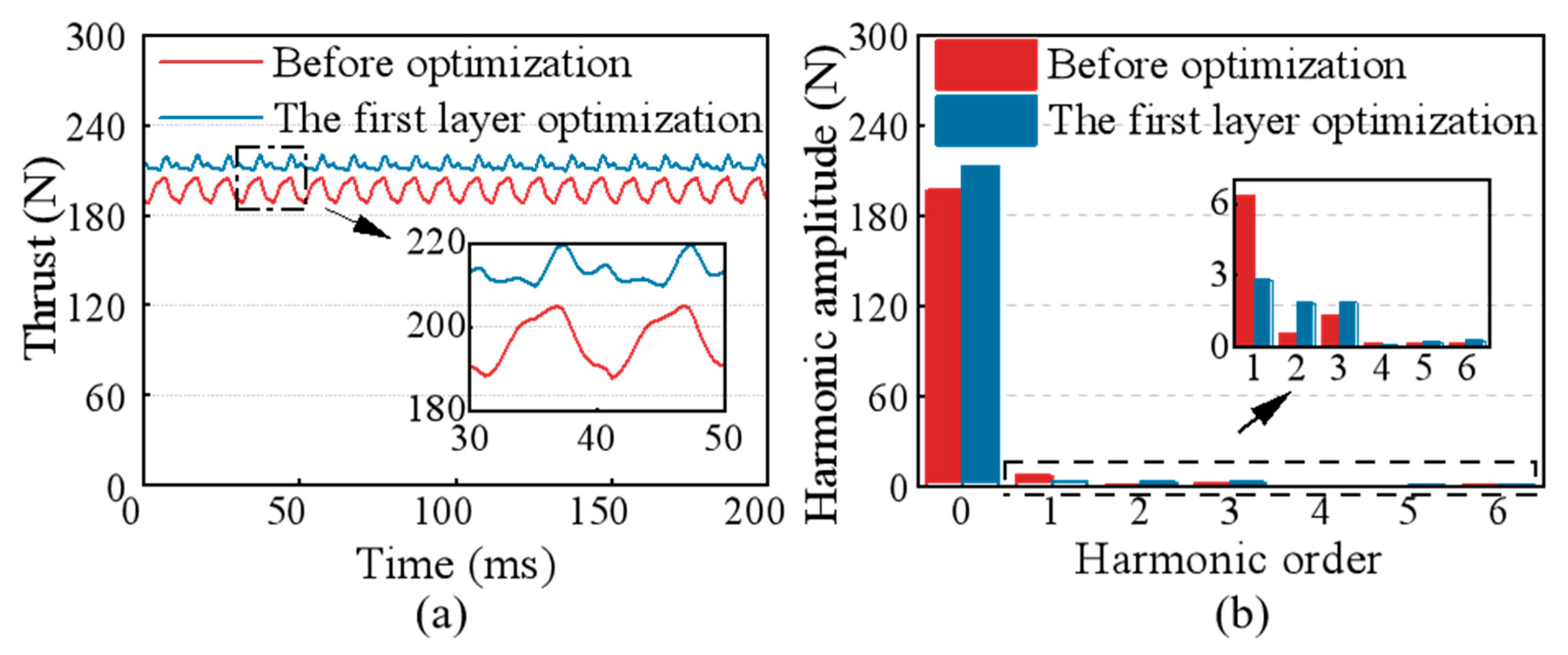
Comparing the motor thrust before and after the first layer optimization, the results are shown in Figure 9. Figure 9a shows the thrust before and after optimization. It can be seen from Figure 9a that the thrust ripple is 8.6% and the average thrust is 196.8 N before optimization. Due to the increase in permanent magnets after optimization, the average thrust is increased, but the thrust ripple is reduced by 40.7%. To further explore the change in harmonic content before and after optimization, the motor thrust is decomposed by Fourier, and the results are shown in Figure 9b. It can be seen from Figure 9b that after optimization, the DC component increases, the first harmonic content decreases significantly, and the second and third harmonic contents increase a little. According to (4), the fundamental component of the end force F_end depends on the Fourier coefficients f_s1 and f_c1. Optimizing w_e changes the end field distribution, thereby reducing the fundamental related coefficients in (4), which causes the decrease in the 1st harmonic in Figure 9b.

3.3. The Second Layer Optimization Based on MOPs

The second optimization process is similar to the first optimization process, which will not be described here. MOPs of average thrust and thrust ripple are shown in Figure 10 and Figure 11. It can be seen from Figure 10 and Figure 11 that the prediction accuracy coefficient of the MOPs of the average thrust is 93%, and the prediction accuracy coefficient of the MOPs of the thrust ripple model is 95%.

Multi-objective PSO is used to optimize the MOPs. The second layer optimization process and Pareto frontier are shown in Figure 8b. A low thrust ripple design scheme is selected: the numbers of turns in phases A, B, and C are 70, 71, and 67, respectively, resulting in a thrust ripple of 3.4% and an average thrust of 214.4 N. Compared with the motor thrust before and after the second layer parameter optimization, the results are shown in Figure 12. As shown in Figure 12a, the average thrust increases and the thrust ripple decreases after optimization. It can be seen from Figure 12b that after optimization, the DC component increases, the primary harmonic content decreases significantly, and other harmonics are almost unchanged.

3.4. The Third Layer Optimization Based on Multi-Objective Taguchi Method

The structural parameters of the third layer optimization are N and θ. Considering that the calculation time is too long and it is inconvenient to modify the parameters of the 3-D finite element model and the rated low-to-medium operating speed of the proposed PMSLM, the segmented skewed pole design method based on the 2-D analytical model is adopted. The residual 3-D discrepancy is therefore neglected in this study. In order to achieve both optimization effect and optimization efficiency, the multi-objective Taguchi method was used for optimization. By superimposing the simulation results of 2-D models, the performance indexes of the segmented skewed pole PMSLM are approximated. The structural parameters of the sub-motor are first determined, and then the thrust of the sub-motor is obtained by changing the primary position of the motor according to the value of N. Finally, the thrust of the motor is obtained by superposing the thrust of the sub-motor.

Considering that the third layer optimization involves the superposition of 2-D finite element models, the multi-objective Taguchi optimization method is adopted in order to achieve both optimization effect and optimization efficiency. An orthogonal table with two parameters and four levels is established, and each set of parameters in the table is substituted into the offset distance calculation formula to find the offset distance x under different oblique pole designs. It can be expressed as

$$x=\tau \cdot {\displaystyle \frac{A}{(N-1)\cdot 180^{°}}}$$

(21)

The thrust ripple and average thrust corresponding to different segmented-skew parameters are evaluated and substituted into the objective function. The candidate design that yields the minimum objective value is selected as the final scheme. It should be noted that the skew design introduces an explicit trade-off between thrust ripple and average thrust. Compared with the result of the second layer optimization, 214.4 N average thrust with 3.4% ripple, the final skewed design significantly suppresses the ripple to 1.2% but reduces the average thrust to 196.1 N. In the final design, N = 4 and θ = 75°, representing a balanced compromise solution under the equal-weight objective.

Compared with the motor thrust before and after the third layer parameter optimization, the results are shown in Figure 13. It can be seen from Figure 13a that after the inclined pole design, the average thrust is significantly reduced, but the thrust ripple is also significantly reduced. It can be seen from Figure 13b that after optimization, the DC component decreases and the first harmonic content increases, but the second and third harmonic contents significantly decrease, and the higher harmonics are almost completely weakened.

The structural parameters of the motor before and after optimization are shown in

Table 4. The structural parameters of the motor before and after optimization.

Items	Initial Value	Optimization Results
Primary core height (mm)	14	14
Primary core length (mm)	150	145
Tooth width (mm)	5.87	6.37
Slot width (mm)	5.8	5.3
Slot height (mm)	11	11
Air gap (mm)	1	1
Secondary core yoke thickness (mm)	3	3
Secondary core length (mm)	140/modular	140/modular
Pole pitch of permanent magnet (mm)	10	10
Permanent magnet width (mm)	8.7	8.7
Pole height of permanent magnet (mm)	2	2.5
Effective length (mm)	55	55

. The average thrust of the motor changes from 196.8 N to 196.1 N, and the thrust ripple decreases from 8.6% to 1.2%, which decreases by 86.0%.

4. Performance Analysis of Optimization Design

4.1. No-Load Performance

4.1.1. No-Load EMF

The comparison of the no-load EMF waveform and its harmonic distribution before and after optimization is shown in Figure 14. It can be seen from Figure 14a that the amplitude of the EMF is basically unchanged before and after optimization. It can be seen from Figure 14b that the first harmonic amplitude is 23.49 V, which slightly increases compared with that before optimization. The third harmonic amplitude is 0.44 V, which is significantly reduced compared with that before optimization, and other harmonics are almost completely weakened.

4.1.2. Detent Force

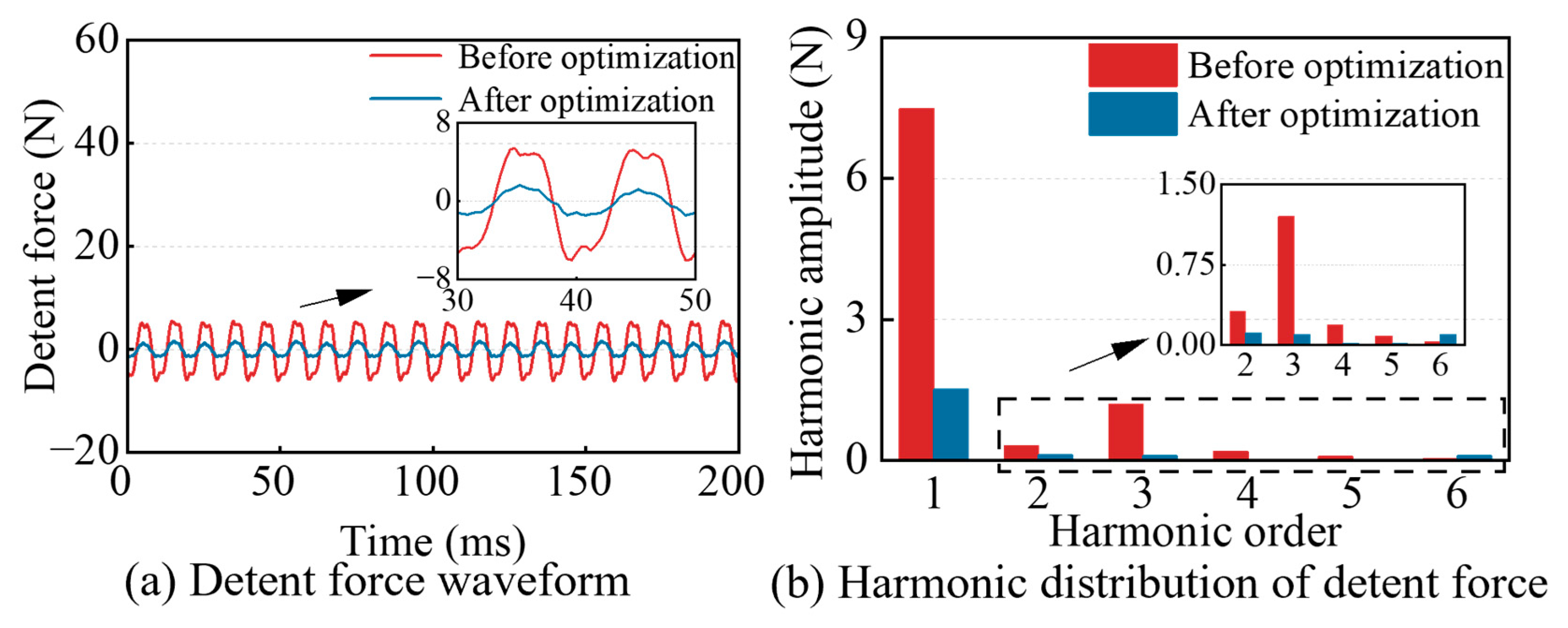
The end force and cogging force of PMSLM are collectively referred to as detent force. The comparison of the detent force waveform and its harmonic distribution before and after optimization is shown in Figure 15. It can be seen from Figure 15a that the peak value of detent force after optimization decreases from 11.69 N to 1.99 N, so the thrust ripple is greatly weakened. It can be seen from Figure 15b that after optimization, the amplitudes of the first, second, and third harmonics are 1.39 N, 0.12 N, and 0.10 N, respectively, and the harmonic content is greatly reduced.

4.2. Load Performance

The comparison of the load thrust waveform and its harmonic distribution before and after optimization is shown in Figure 16. It can be seen from Figure 16a that the peak-to-peak value of thrust after optimization is 2.35 N, which is greatly reduced compared with that before optimization. It can be seen from Figure 16b that after optimization, the amplitudes of the DC component, the first harmonic, and the third harmonic are 195.97 N, 1.20 N, and 0.10 N, respectively. The DC component is almost unchanged, but the first and third harmonic amplitudes are reduced by 5.14 N and 1.17 N, respectively, so the thrust ripple is reduced from 8.6% to 1.2%.

5. Experimental Verification

5.1. Prototype Motor and Experimental Platform

A three-closed-loop control strategy of position, speed, and current is adopted, and the system experiment platform is built on this basis, as shown in Figure 17. It can be seen from Figure 17 that the experimental platform is mainly composed of an industrial personal computer, hardware in the loop controller (National Instruments, Austin, TX, USA), transfer port, power supply (Uni-trend Technology Co., Ltd., Dongguan, China), auxiliary power (Shenzhen Mastech Electronics Co., Ltd., Shenzhen, China), drive circuit, segmented skewed pole PMSLM, weighing sensor (Bengbu Dayang Sensing System Engineering Co., Ltd., Bengbu, China), weighing transmitter (Bengbu Dayang Sensing System Engineering Co., Ltd., Bengbu, China), and oscilloscope (Shide Technology Co., Ltd., Santa Rosa, CA, USA). The software used is EasyGo PESuite 22.0.0.1. The primary is connected to a force weighing sensor.

5.2. No-Load Experiment

To improve the accuracy of the no-load experiment, the motor is controlled to move at 4 different speeds v, and the line no-load EMF is shown in Figure 18. It can be seen from Figure 18 that the sinusoidal properties of line no-load EMF are good when running with 4 different v.

The effective values of the motor EMF under different v are obtained. The EMF constant is the ratio of the root mean square (RMS) of the EMF to the velocity, and the average value of the EMF constant of the motor is obtained. The results are shown in

Table 5. No-load EMF at different v.

	Experimental Results		Simulation Results
	EMF (V)	EMF Constant (V/m/s)	EMF (V)	EMF Constant (V/m/s)
70 mm/s	1.11	15.86	1.18	16.86
85 mm/s	1.35	15.88	1.41	16.59
100 mm/s	1.56	15.60	1.67	16.70
115 mm/s	1.79	15.57	1.92	16.70
Average	/	15.73	/	16.71

. It can be seen from Table 5 that the average value of the EMF constant in the experiment is 15.73 V/m/s, while the average value of the EMF constant in the simulation is 16.71 V/m/s, with an error of 5.86%. There are two main reasons for the error: one is that during the processing and installation process, the air gap between the primary and secondary is not completely uniform, and the other is that the permanent magnet is not completely uniform.

5.3. Load Experiment

To measure the thrust of the motor, the primary is energized to a uniform motion and connected with load F_L. The thrust of the motor is the resultant force measured by the weighing sensor and the friction force exerted by the movement of the motor, which has been measured by a no-load experiment and is 9.90 N in forward motion. To improve the accuracy of the load test, the motor A is connected with the F_L of 1 kg, 2 kg, 3 kg, and 5 kg, and runs at 50 mm/s. The three-phase current i_A, i_B, and i_C of the motor under different loads are shown in Figure 19. It can be seen from Figure 19 that the RMS I of the phase current under the F_L of 1 kg, 2 kg, 3 kg, and 5 kg is 0.61 A, 0.80 A, 1.07 A, and 1.52 A, respectively, and the amplitude of the three-phase current is different because the primary end of the motor is disconnected.

The thrust measured by load sensors under different loads is shown in Figure 20, Figure 21, Figure 22 and Figure 23. It can be seen from Figure 20, Figure 21, Figure 22 and Figure 23 that the periodicity of thrust under different loads is the same. When the load is moving forward, the average force measured by the weighing sensor under the F_L of 1 kg, 2 kg, 3 kg, and 5 kg is 19.88 N, 28.97 N, 43.07 N, and 64.00 N, respectively.

Therefore, when the F_L is 1 kg, 2 kg, 3 kg, and 5 kg, the average thrust of motor A is 29.78 N, 38.87 N, 52.97 N, and 73.90 N, respectively. The thrust constant is the ratio of the average thrust to I of the three-phase winding current of motor A. The average value of the thrust constant is shown in

Table 6. Thrust under different F_L.

	Experimental Results		Simulation Results
	Thrust (N)	Thrust Constant (N/A)	Thrust (N)	Thrust Constant (N/A)
0.61 A	29.78	48.82	31.32	51.19
0.80 A	38.87	48.59	40.56	50.70
1.07 A	52.97	49.50	55.15	51.54
1.52 A	73.90	48.62	77.31	50.86
Average	/	48.88	/	51.07

. It can be seen from Table 6 that the average value of the thrust constant in the experiment is 48.88 N/A, and that in the simulation is 51.07 N/A, with an error of 4.29%. It is mainly caused by the error generated during processing and the error generated by the measuring instrument.

From Figure 20b, Figure 21b, Figure 22b, and Figure 23b, it can be seen that the variation trend of PMSLM speed waveform is the same when the load F_L is 1 kg, 2 kg, 3 kg, and 5 kg, the thrust ripples are 2.64%, 2.86%, 3.10%, and 3.50%, respectively. Compared with the no-load operation, as the load F_L increases, the thrust ripple gradually increases. In addition to the influence of measurement error, the asymmetric effect of PMSLM winding intensifies with the increase in current under load, which leads to an increase in thrust ripple.

6. Conclusions

This study proposes a layered multi-objective optimization design method based on the analysis of the thrust ripple of the segmented skewed pole PMSLM. The influence patterns of end force, cogging force, and winding asymmetry force on thrust ripple are analyzed and obtained by using a 2-D analytical model. On the basis of determining the key structural parameters, a three-layered multi-objective optimization is conducted for the PMSLM. The simulation results indicate that the thrust ripple is reduced from 8.6% to 1.2%, corresponding to an 86.0% reduction. Subsequently, the prototype experiment is carried out by building a test platform. The no-load EMF constant and thrust constant are obtained based on the experimental data, and the errors between them and the simulation results are 5.86% and 4.29%, respectively. The experimental results verify that the thrust ripple analysis and the layered multi-objective optimization method presented in this study are correct and effective. In addition, this method shows potential for other devices.

References

1. Konuhova, M. Induction motor dynamics regimes: A comprehensive study of mathematical models and validation. Appl. Sci. 2025, 15, 1527. [Google Scholar] [CrossRef]
2. Vlachou, V.; Sakkas, G.; Xintaropoulos, F.; Pechlivanidou, M.; Kefalas, T.; Tsili, M.; Kladas, A. Overview on permanent magnet motor trends and developments. Energies 2024, 17, 538. [Google Scholar] [CrossRef]
3. Gherghina, I.; Bizon, N.; Iana, G.; Vasilică, B. Recent advances in fault detection and analysis of synchronous motors: A review. Machines 2025, 13, 815. [Google Scholar] [CrossRef]
4. He, Z.; Dong, F.; Zhao, J.; Wang, L.; Song, J.; Song, X. Thrust Ripple Reduction in Permanent Magnet Synchronous Linear Motor Based on Electromagnetic Damping-Spring System. IEEE Trans. Energy Convers. 2018, 33, 2122–2132. [Google Scholar] [CrossRef]
5. Lei, G.; Liu, C.; Li, Y.; Chen, D.; Guo, Y.; Zhu, J. Robust Design Optimization of a High-Temperature Superconducting Linear Synchronous Motor Based on Taguchi Method. IEEE Trans. Appl. Supercond. 2019, 29, 1–6. [Google Scholar] [CrossRef]
6. Guo, R.; Yu, H.; Guo, B. Analysis of a Tubular Linear Permanent Magnet Oscillator With Auxiliary Teeth Configuration for Energy Conversion System. IEEE Trans. Transp. Electrif. 2020, 6, 602–611. [Google Scholar] [CrossRef]
7. Hu, H.; Zhao, J.; Liu, X.; Guo, Y.; Zhu, J. No-Load Magnetic Field and Cogging Force Calculation in Linear Permanent-Magnet Synchronous Machines with Semiclosed Slots. IEEE Trans. Ind. Electron. 2017, 64, 5564–5575. [Google Scholar] [CrossRef]
8. Xie, Z.; Lu, Q.; Mei, W.; Li, Y. Improved Analytical Modeling of a Novel Ironless Linear Synchronous Machine with Asymmetrical Double-Layer Winding Topology. IEEE Trans. Ind. Appl. 2021, 57, 1411–1419. [Google Scholar] [CrossRef]
9. Cisse, K.M.; Nasr, A.; Chareyron, B.; Abdelli, A.; Milosavljevic, M. Surrogate model-based optimization methodology for high torque and power density permanent magnet assisted synchronous reluctance motor. In Proceedings of the 2022 International Conference on Electrical Machines (ICEM), Valencia, Spain, 5–8 September 2022; IEEE: New York, NY, USA, 2022; pp. 295–301. [Google Scholar]
10. Sun, C.; Li, Q.; Fan, T.; Wen, X.; Li, Y. Multi-objective optimization design of external rotor permanent magnet machine for in-wheel applications. In Proceedings of the 2023 24th International Conference on the Computation of Electromagnetic Fields (COMPUMAG), Kyoto, Japan, 22–26 May 2023; IEEE: New York, NY, USA, 2023; pp. 1–4. [Google Scholar]
11. Liu, X.; Hu, C.; Li, X.; Gao, J.; Huang, S. An Online Data-Driven Multi-Objective Optimization of a Permanent Magnet Linear Synchronous Motor. IEEE Trans. Magn. 2021, 57, 1–4. [Google Scholar] [CrossRef]
12. Hasanien, H.M. Particle swarm design optimization of transverse flux linear motor for weight reduction and improvement of thrust force. IEEE Trans. Ind. Electron. 2011, 58, 4048–4056. [Google Scholar]
13. Lei, G.; Xu, W.; Hu, J.; Zhu, J.; Guo, Y.; Shao, K. Multilevel design optimization of a FSPMM drive system by using sequential subspace optimization method. IEEE Trans. Magn. 2014, 50, 685–688. [Google Scholar] [CrossRef]
14. Xia, C.; Guo, L.; Zhang, Z.; Shi, T.; Wang, H. Optimal designing of permanent magnet cavity to reduce iron loss of interior permanent magnet machine. IEEE Trans. Magn. 2015, 51, 1–9. [Google Scholar] [CrossRef]
15. Mei, J.; Zuo, Y.; Lee, C.H.T.; Kirtley, J.L. Modeling and optimizing method for axial flux induction motor of electric vehicles. IEEE Trans. Veh. Technol. 2020, 69, 12822–12831. [Google Scholar] [CrossRef]
16. Lei, G.; Wang, T.; Zhu, J.; Guo, Y.; Wang, S. System-level design optimization method for electrical drive systems—Robust approach. IEEE Trans. Ind. Electron. 2015, 62, 4702–4713. [Google Scholar] [CrossRef]
17. Pu, W.; Quan, L.; Xiang, Z.; Zhu, X.; Xue, G. Multiharmonic-layered design and optimization of a flux-concentrated PM vernier motor considering harmonic sensitivity. IEEE Trans. Transp. Electrif. 2024, 10, 648–659. [Google Scholar] [CrossRef]
18. Huang, X.; Tan, Q.; Wang, Q.; Li, J. Optimization for the pole structure of slot-less tubular permanent magnet synchronous linear motor and segmented detent force compensation. IEEE Trans. Appl. Supercond. 2016, 26, 1–5. [Google Scholar] [CrossRef]
19. Zhu, X.; Yang, J.; Xiang, Z.; Jiang, M.; Zheng, S.; Quan, L. Robust-Oriented Optimization Design for Permanent Magnet Motors Considering Parameter Fluctuation. IEEE Trans. Energy Convers. 2020, 35, 2066–2075. [Google Scholar] [CrossRef]
20. Zhu, X.; Fan, D.; Xiang, Z.; Quan, L.; Hua, W.; Cheng, M. Systematic multi-level optimization design and dynamic control of less-rare-earth hybrid permanent magnet motor for all-climatic electric vehicles. Appl. Energy 2019, 253, 113549. [Google Scholar] [CrossRef]
21. Ma, B.; Lei, G.; Zhu, J.; Guo, Y.; Liu, C. Application-oriented robust design optimization method for batch production of permanent-magnet motors. IEEE Trans. Ind. Electron. 2018, 65, 1728–1739. [Google Scholar] [CrossRef]
22. Sun, X.; Shi, Z.; Lei, G.; Guo, Y.; Zhu, J. Multi-objective design optimization of an IPMSM based on multilevel strategy. IEEE Trans. Ind. Electron. 2021, 68, 139–148. [Google Scholar] [CrossRef]
23. Xiang, Z.; Zhu, X.; Quan, L.; Du, Y.; Zhang, C.; Fan, D. Multilevel design optimization and operation of a brushless double mechanical port flux-switching permanent-magnet motor. IEEE Trans. Ind. Electron. 2016, 63, 6042–6054. [Google Scholar] [CrossRef]
24. Zhao, S.; Blaabjerg, F.; Wang, H. An overview of artificial intelligence applications for power electronics. IEEE Trans. Power Electron. 2021, 36, 4633–4658. [Google Scholar] [CrossRef]
25. Gu, J.; Hua, W.; Yu, W.; Zhang, Z.; Zhang, H. Surrogate model-based multiobjective optimization of high-speed PM synchronous machine: Construction and comparison. IEEE Trans. Transp. Electrif. 2023, 9, 678–688. [Google Scholar] [CrossRef]
26. Zhang, J.; Yan, J.; Chi, S.; Zhou, Y.; Ying, Z. Multi-objective optimization design of single side flat tooth unequal width permanent magnet synchronous linear motor based on layered strategy. J. Nanjing Univ. Sci. Technol. 2023, 47, 571–578. [Google Scholar]
27. Li, B.; Zhang, Z.; Gao, P.; Yuan, Y.; Li, G. Optimized design of micro-joint motors using MPSO with embedded ELM indirect surrogate. IEEE Trans. Energy Convers. 2024, 39, 1314–1324. [Google Scholar] [CrossRef]
28. Ibrahim, I.; Silva, R.; Lowther, D.A. Application of surrogate models to the multiphysics sizing of permanent magnet synchronous motors. IEEE Trans. Magn. 2022, 58, 1–4. [Google Scholar] [CrossRef]
Figure 1. The topology of the segmented skewed pole PMSLM.
Applsci 16 00969 g001
Figure 2. The FEA verification of cogging force analysis. (a) Waveforms. (b) Harmonics.
Applsci 16 00969 g002
Figure 3. The mechanism of the layered multi-objective optimization method.
Applsci 16 00969 g003
Figure 4. Parameter sensitivity. (a) Thrust ripple SNR. (b) Sensitivity analysis showing the three most sensitive parameters are we, hm, and ws.
Applsci 16 00969 g004
Figure 5. The generation process of the MOP.
Applsci 16 00969 g005
Figure 6. MOPs of average thrust in the first layer optimization. (a) we = 2.935 mm. (b) ws = 5.8 mm. (c) hm = 2 mm.
Applsci 16 00969 g006
Figure 7. MOPs of thrust ripple in the first layer optimization. (a) we = 2.935 mm. (b) ws = 5.8 mm. (c) hm = 2 mm.
Applsci 16 00969 g007
Figure 8. Optimization processes and Pareto frontiers. (a) First layer. (b) Second layer.
Applsci 16 00969 g008
Figure 9. The motor thrust before and after the first layer optimization. (a) Time-domain waveforms showing reduction in oscillation. (b) Harmonic spectra showing strong suppression of 1st harmonic.
Applsci 16 00969 g009
Figure 10. MOPs of average thrust in the second layer optimization. (a) tC = 69 turns. (b) tB = 69 turns. (c) tA = 69 turns.
Applsci 16 00969 g010
Figure 11. MOPs of thrust ripple in the second layer optimization. (a) tC = 69 turns. (b) tB = 69 turns. (c) tA = 69 turns.
Applsci 16 00969 g011
Figure 12. The motor thrust before and after the second layer optimization. (a) Time-domain waveforms showing an increase in average thrust and a reduction in oscillation. (b) Harmonic spectra showing an increase in DC component and strong suppression of the 1st harmonic.
Applsci 16 00969 g012
Figure 13. The motor thrust before and after the third layer optimization. (a) Time-domain waveforms showing a reduction in both the average thrust and thrust oscillations. (b) Harmonic spectra showing suppression of the DC, 2nd-, 3rd-, and higher-order components, while the 1st harmonic slightly increases.
Applsci 16 00969 g013
Figure 14. The comparison of no-load EMF waveform and its harmonic distribution before and after optimization. (a) Time-domain waveforms showing a basically unchanged EMF. (b) Harmonic spectra showing a slight increase in 1st harmonic and a reduction in other harmonics.
Applsci 16 00969 g014
Figure 15. The comparison of the detent force waveform and its harmonic distribution before and after optimization. (a) Time-domain waveforms showing a significant reduction in thrust ripple. (b) Harmonic spectra showing strong suppression of all harmonics.
Applsci 16 00969 g015
Figure 16. The comparison of the load thrust waveform and its harmonic distribution before and after optimization. (a) Time-domain waveforms showing a significant reduction in thrust ripple. (b) Harmonic spectra showing a basically unchanged DC component and a reduction of the 1st and 3rd harmonics.
Applsci 16 00969 g016
Figure 17. Experimental platform. (a) Overall structure of the experimental platform. (b) Loading plan.
Applsci 16 00969 g017
Figure 18. Characteristics of no-load EMF under different v. (a) v = 70 mm/s. (b) v = 85 mm/s. (c) v = 100 mm/s. (d) v = 115 mm/s.
Applsci 16 00969 g018
Figure 19. Three-phase current under different FL. (a) FL = 1 kg. (b) FL = 2 kg. (c) FL = 3 kg. (d) FL = 5 kg.
Applsci 16 00969 g019
Figure 20. Thrust measured by the weighting sensor when FL = 1 kg. (a) Thrust measured by the weighting sensor. (b) Local enlarged drawing.
Applsci 16 00969 g020
Figure 21. Thrust measured by the weighting sensor when FL = 2 kg. (a) Thrust measured by the weighting sensor. (b) Local enlarged drawing.
Applsci 16 00969 g021
Figure 22. Thrust measured by the weighting sensor when FL = 3 kg. (a) Thrust measured by the weighting sensor. (b) Local enlarged drawing.
Applsci 16 00969 g022
Figure 23. Thrust measured by the weighting sensor when FL = 5 kg. (a) Thrust measured by the weighting sensor. (b) Local enlarged drawing.
Applsci 16 00969 g023