Research on a Wave Elevation Reconstruction Method at Fixed Positions

Abstract

Accurate wave detection is essential for reliable ship motion prediction and the safety of offshore operations. Wave buoys are widely deployed as key instruments for capturing wave characteristics. However, buoys drift due to the waves and currents, resulting in errors in reconstructed wave elevation. To address this challenge, a fixed-position wave-elevation reconstruction method is proposed in this paper. First, a temporal convolutional network (TCN) module is integrated with a gated recurrent unit (GRU) network to efficiently capture the nonlinear relationship between buoy motion and wave elevation, enabling simultaneous wave elevation reconstruction and dynamic deviation compensation. Second, a static deviation compensation algorithm developed from wave theory is introduced to convert the spatial deviation into temporal misalignment. The proposed method is evaluated in both time and frequency domains across various sea conditions. Results demonstrate that the proposed method effectively compensates for deviations and achieves accurate reconstruction of wave elevation at the target position. In higher sea states, accurate reconstruction is maintained even at large static deviations, with relative errors typically within 10–15%. Frequency-domain analysis shows that coherence approaches 1 near the spectral peak and below 0.3 at higher frequencies, indicating that the dominant wave components are accurately reconstructed and that high-frequency noise has a limited impact on overall accuracy.

1. Introduction

The motion response of a ship mainly depends on the instantaneous attitude and incident waves to the hull. During offshore operations, the attitude of the ship varies instantaneously due to the wind and waves, directly affecting operational stability and safety [1]. Accurate detection and characterization of ocean waves can enhance the efficiency of maritime operations and reduce the risk of accidents [2]. Reliable wave reconstruction techniques are thus needed for selecting appropriate operational strategies and compensating for ship motion.

Waves are a fundamental component of the ocean environment that are generated by natural factors such as wind forcing and the Earth’s rotation [3]. Advanced wave detection technologies enable real-time acquisition of wave height, frequency, direction, and other critical parameters [4,5]. By integrating the ship motion, more precise and longer-term motion forecasting models can be developed [6]. In a complex and dynamic marine environment, the ability to issue timely warnings for excessive ship motions not only reduces operational risk but also improves operational efficiency. However, the temporal evolution of wave elevation at a fixed position cannot be directly measured and must instead be inferred through ocean-sensing devices in practical ocean settings.

Wave buoys, which measure sea-surface motion by following the vertical displacements of waves, are widely used to obtain wave height, peak periods, and wave spectra. Equipped with accelerometers or inclinometers, wave buoys record vertical acceleration or attitude variations and estimate significant wave height, mean period, and spectral properties through spectral analysis in the frequency domain, typically using the fast Fourier transform (FFT) [7]. Previous studies have demonstrated the feasibility of estimating the spatial wave field by deploying multiple buoys to collect time series observations [8,9,10]. Additional research has further integrated drifting buoys and GNSS-based techniques to enable real-time wave measurements. Liu et al. conducted high-precision real-time online reconstruction of waves based on the segmented wave parameter method of Global Navigation Satellite System (GNSS) wave buoys [11]. Herbers et al. monitored wave surfaces using a Global Positioning System (GPS)-assisted Datawell buoy, finding that Datawell GPS buoys could better estimate wave frequency and directional spectra under benign swell conditions compared to traditional accelerometer–compass Datawell buoys [12].

In recent years, several studies have combined machine learning techniques with physics-based models to reconstruct and predict wave fields from sparse or simulated observations [13,14,15]. More generally, physics-informed neural network approaches provide a principled way to embed governing equations and boundary conditions into learning architectures [16]. These works demonstrate the theoretical and practical feasibility of using machine learning when coupled with physical knowledge to recover wave elevation time histories from limited measurements. Treating buoy motion responses as a viable data source for fixed-position wave reconstruction is well supported by recent hybrid physics–ML advances. Some neural network methods have been applied to wave reconstruction tasks. Desouky et al. used a nonlinear autoregressive neural network model (NARX), combined with the Waverider buoy, to predict the wave elevation [17]. Qin et al. used artificial neural networks (ANNs) to reconstruct wave elevation time series based on a self-navigating buoy, and achieved good results [18]. Nielsen et al. used three different machine learning models to process the motion response data of the buoy, and characterized the sea state in different ways [19].

Despite the advantages, wave buoys are susceptible to positional deviations caused by the combined influence of waves and ocean currents. Wind or current forcing can induce drift, while wave-induced motions lead to vertical oscillations and horizontal displacements [20]. Such deviations introduce amplitude and phase errors into the wave-reconstruction process, thereby reducing the accuracy of wave-height reconstruction.

To address this challenge, a wave elevation reconstruction method specifically designed for fixed-position is proposed. This method estimates the wave elevation time series at a target geographical position from the measured motion response of a drifting buoy. The deviation for buoys is divided into two parts: dynamic deviation and static deviation. The proposed framework assumes that, within the limited drift range typically encountered, dominant wave characteristics remain effectively unchanged across the spatial domain. First, a TCN module is integrated with a GRU network to efficiently capture the nonlinear relationship between buoy motion and wave elevation, enabling simultaneous wave elevation reconstruction and dynamic deviation compensation. Second, based on wave theory under the premise of smooth spatial evolution of the wave field, a static deviation compensation model is developed to convert the spatial displacement into temporal misalignment. A time series prediction model is then employed to reconstruct the incident wavefront. The overall framework of the proposed method is illustrated in Figure 1.

2. Materials and Methods

2.1. Wave-Induced Buoy Motion Response

When subjected to wave action, a buoy exhibits multi-degree-of-freedom (multi-DOF) motions. Typically, the wave-induced forces manifest as time-varying loads that depend on wave height and period, causing the buoy’s response to exhibit pronounced frequency dependence and nonlinear features. The generalized displacement vector of the buoy is determined using Equation (1):

$$\begin{array}{c}q\left(t\right)={\left[\begin{array}{cc}\begin{array}{ccc}x\left(t\right)& y\left(t\right)& z\left(t\right)\end{array}& \begin{array}{ccc}\varphi \left(t\right)& \theta \left(t\right)& \psi \left(t\right)\end{array}\end{array}\right]}^T\end{array}$$

(1)

Under the small-amplitude motion assumption, the mooring line restoring force can be linearized into an equivalent stiffness form. Accordingly, the mooring-induced forces can be represented as a combination of added mass M, damping C, and stiffness K. For a single-anchor gravity-type buoy, the mooring force $F_m$ generally depends on the buoy displacement and velocity in Equation (2).

$$\begin{array}{c}{F}_m\approx -K_{m}q\left(t\right)-C_m\dot{q}\left(t\right)\end{array}$$

(2)

where $K_m\in {\mathbb{R}}^{6\times 6}$ and $C_m\in {\mathbb{R}}^{6\times 6}$ denote the equivalent mooring stiffness and damping matrices, respectively. By retaining the wave excitation, the linearized motion equation of a single-anchor gravity-type buoy can be expressed as Equation (3).

$$\begin{array}{c}{M}_b\ddot{q}\left(t\right)+C\left(\omega \right)\dot{q}\left(t\right)+Kq\left(t\right)=F_w\left(t\right)\end{array}$$

(3)

where $M_b\in {\mathbb{R}}^{6\times 6}$ is the buoy mass matrix including added mass; $C\in {\mathbb{R}}^{6\times 6}$ is the frequency-dependent matrix combining radiation and viscous damping; $K\in {\mathbb{R}}^{6\times 6}$ is the effective stiffness matrix resulting from both mooring line and hydrostatic restoring forces; and $F_w\in {\mathbb{R}}^{6\times 1}$ represents the wave-induced forces and moments in 6-DOF. All major symbols used in this study are defined and summarized in

Table 1. Table of symbols.

Symbol	Description	Symbol	Description
$q\left(t\right)$	Buoy generalized displacement vector	$\overline{u}$	Mean horizontal fluid speed
$F_m$	Mooring force	$ϵ$	Dimensionless wave amplitude
$K_m$	Equivalent mooring stiffness	c	Wave speed
$C_m$	Equivalent damping matrices	L	Wave length
$C\left(\omega \right)$	Frequency-dependent matrix	$k$	Wave number
$M_b$	Buoy mass matrix	$C_0$, $C_2$, $C_4$	Dimensionless coefficients
$F_w\left(t\right)$	Wave-induced forces/moments	${\tau }_{od}$	Time steps for prediction
${\overrightarrow{R}}_{od}$	Static deviation	$h_o$	Wave elevation at the target position
${\overrightarrow{R}}_{da}$	Dynamic deviation	$c_E$	Eulerian time mean fluid velocity
$\delta$	Attenuation coefficient	$f_s$	Sampling frequency
$U_r$	Ursell number	$f_k$	Discrete frequency

.

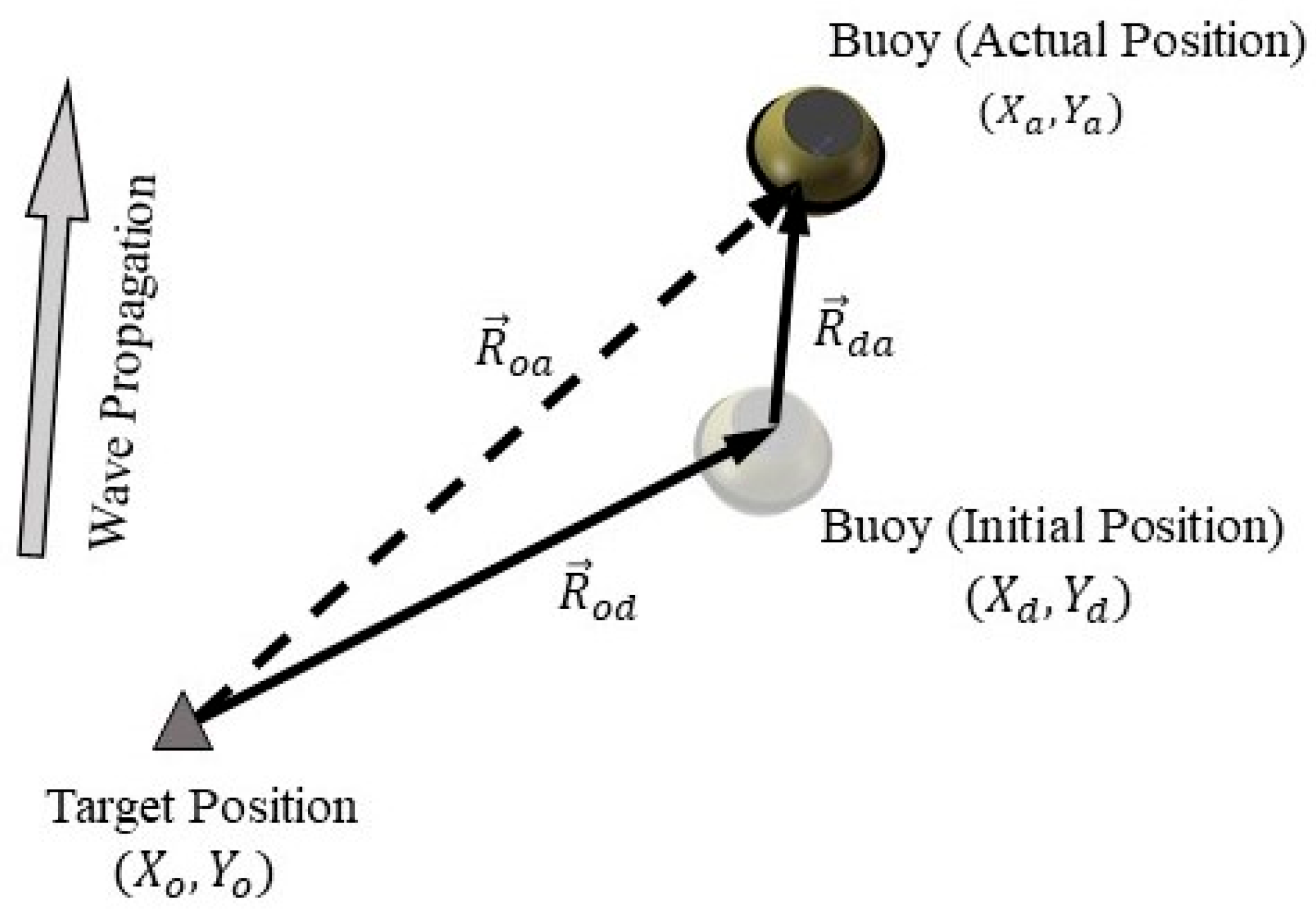
Affected by waves and currents, the position of a buoy constantly changes, resulting in positional deviations between the buoy and the target position. When monitoring waves with a gravitational moored buoy, the actual position of the buoy $(X_a,Y_a)$ always deviates from the target position $(X_o,Y_o)$ by a certain deviation ${\overrightarrow{R}}_{oa}$. As shown in Figure 2 and Equation (4), the deviation can be divided into two parts: static deviation ${\overrightarrow{R}}_{od}$ and dynamic deviation ${\overrightarrow{R}}_{da}$. Static deviation refers to the difference between the buoy’s still-water position $(X_d,Y_d)$ and the target position $(X_o,Y_o)$, caused by operational errors during deployment or the environmental conditions. Dynamic deviation refers to the buoy’s position changes under the influence of waves, wind, and other external environmental factors, which is a time variable. Positional deviation causes amplitude and phase errors in the reconstructed wave elevation.

$$\begin{array}{c}{\overrightarrow{R}}_{oa}={\overrightarrow{R}}_{od}+{\overrightarrow{R}}_{da}\end{array}$$

(4)

To achieve accurate wave elevation reconstruction at a target spatial position, it is necessary to compensate for the positional deviation of the drifting buoy. The proposed deviation compensation framework consists of two components: static deviation compensation and dynamic deviation compensation.

The static deviation compensation relies on several physical assumptions that are reasonable over short spatial scales and limited time intervals. First, within the buoy drift range, the local water depth d and seabed topography are assumed to vary slowly, such that their influence on the linear wave dispersion relation can be neglected. As a result, the dispersion characteristics of the wave field are approximately identical at the buoy position $(X_d,Y_d)$ and the target position $(X_o,Y_o)$. Second, the dominant wave propagation direction and phase speed are assumed to remain approximately constant over the short prediction horizon considered in this study. Under this assumption, the spatial offset between the buoy and the target location can be equivalently mapped to a temporal delay through the local wave phase speed. Finally, the wave field is assumed to be dominated by low- to moderate-frequency components, for which linear or weakly nonlinear wave theory provides an adequate first-order description of wave phase evolution and amplitude attenuation over short propagation distances. Based on these assumptions, the wave speed c, wavelength L, and wave period T at the buoy location are taken to be identical to those at the target position during static deviation compensation. Affected by wave viscous dissipation, the wave height at the target position $H_o$ is given by Equation (5):

$$\begin{array}{c}{H}_o=H_d{e}^{-\delta \left|{\overrightarrow{R}}_{od}\right|}\end{array}$$

(5)

where $H_d$ is the wave height obtained from the reconstruction at the initial position, and $\delta$ is the attenuation coefficient. The Stokes wave theory used in this paper is based on the potential flow theory, ignoring the influence of fluid viscosity. Therefore, for shallow water regular waves, it is also necessary to compensate for the wave loss along the way caused by viscous dissipation. According to the experimental results of Yayi et al., wave attenuation along the path follows an exponential decay, and the attenuation coefficient $\delta$ in regular waves is empirically related to the Ursell number, as shown in Equations (6) and (7) [21].

$$\begin{array}{c}\delta =0.0071U_r^{-0.196}\end{array}$$

(6)

$$\begin{array}{c}{U}_r={\displaystyle \frac{H{L}^2}{d^3}}\end{array}$$

(7)

where the Ursell number comes from the Stokes expansion of nonlinear periodic waves and is a dimensionless parameter measuring wave nonlinearity. The mean horizontal fluid speed $\overline{u}$ for constant-length waves can be obtained from Equation (8):

$$\begin{array}{c}\overline{u}{\left({\displaystyle \frac{k}{g}}\right)}^{{\displaystyle \frac{1}{2}}}=C_0+C_2{ϵ}^2+C_4{ϵ}^4+O\left({ϵ}^6\right)\end{array}$$

(8)

where g is the gravitational acceleration, $ϵ=kH/2$ is the dimensionless wave amplitude. $O\left({ϵ}^6\right)$ is a Landau order symbol, denoting the neglected sixth-order term of $ϵ$. $C_0$, $C_2$, and $C_4$ are dimensionless coefficients of the mean fluid speed, which can be solved using Equations (9)–(11) [22].

$$\begin{array}{c}{C}_0=\sqrt{\tanh \left(kd\right)}\end{array}$$

(9)

$$\begin{array}{c}{C}_2=C_0{\displaystyle \frac{7S^2+2}{4{\left(S-1\right)}^2}}\end{array}$$

(10)

$$\begin{array}{c}{C}_4=C_0{\displaystyle \frac{146S^5-71S^4-400S^3-116S^2+32S+4}{32{\left(S-1\right)}^5}}\end{array}$$

(11)

where $S=\mathrm{s}\mathrm{e}\mathrm{c}\mathrm{h}\left(2kd\right)$. According to Fenton’s theory, the Eulerian time mean fluid velocity $c_E$ is influenced by both the wave speed c and the mean horizontal fluid speed $\overline{u}$ [23]. Wave characteristics can be solved using the fifth-order Stokes wave equation, with wave speed c and Eulerian time mean fluid velocity $c_E$ given by Equations (12) and (13):

$$\begin{array}{c}{c}_E=c-\overline{u}\end{array}$$

(12)

$$\begin{array}{c}c={\displaystyle \frac{2\pi }{kT}}\end{array}$$

(13)

Substituting Equations (9)–(13) into Equation (8), and ignoring the higher-order terms related to ${ϵ}^6$, the transcendental nonlinear equation for the wave number k is derived. By solving Equation (14), the wave speed c can be solved.

$$\begin{array}{c}{c}_E{\left({\displaystyle \frac{k}{g}}\right)}^{{\displaystyle \frac{1}{2}}}={\displaystyle \frac{2\pi }{T{\left(gk\right)}^{\frac{1}{2}}}}-C_0-C_2{\left({\displaystyle \frac{kH}{2}}\right)}^2-C_4{\left({\displaystyle \frac{kH}{2}}\right)}^4\end{array}$$

(14)

In the absence of $c_E$, the wave speed can be approximated using the first-order Stokes wave equation as Equation (15). Assuming $c_E$ is zero due to the relatively small mean current in deep water compared to the typical wave speed. The static deviation is compensated according to the non-attenuated irregular waveform.

$$\begin{array}{c}c={\displaystyle \frac{gT}{2\pi }}\tanh \left(kd\right)\end{array}$$

(15)

Similarly, irregular wave fields are generally parameterized using significant wave height and peak period. The wavelength distribution is essentially determined by the wave energy spectrum through the linear wave dispersion relation. The frequency $\omega$ corresponding to each wavelength L in the wave spectrum can be obtained from Equation (16):

$$\begin{array}{c}\omega =gk\tanh \left(kd\right)\end{array}$$

(16)

The wave elevation and time series are discretized by the sampling time $t_s$ to meet practical engineering needs. The time step length ${\tau }_{od}$ for waves to propagate from the target position to the initial position is determined using Equation (17):

$$\begin{array}{c}{\tau }_{od}=round\left({\displaystyle \frac{{\overrightarrow{R}}_{oa}·{\overrightarrow{R}}_{od}}{c{t}_s·\left|{\overrightarrow{R}}_{oa}\right|}}\right)\end{array}$$

(17)

Under the premise that the dynamic deviation ${\overrightarrow{R}}_{oa}$ direction along the wave propagation, the wave at the target position at time $t$ can be regarded as the wave at the buoy after $t_s{·\tau }_{od}$ with viscous dissipation. Therefore, the deviation compensation for the target wave elevation can be regarded as a time series prediction task from the wave elevation at the initial position. The reconstruction at the target position at $t$ is converted into the prediction of the wave elevation at the initial position after ${\tau }_{od}$ time steps. The wave elevation $h_o$ at the target position at time $t$ can be obtained using Equation (18):

$$\begin{array}{c}{h}_o\left(t\right)=Y\left({\tau }_{od}\right)·e^{-\delta \left|{\overrightarrow{R}}_{od}\right|}\end{array}$$

(18)

where $Y$ is the time series prediction model, and $Y\left({\tau }_{od}\right)$ is the time series prediction result with ${\tau }_{od}$ time steps. The time series prediction is performed based on the wave elevation at the initial position, which is obtained by dynamic deviation compensation.

2.2. TCN-GRU Network

The static deviation compensation for wave elevation is based on the results of dynamic deviation compensation. Effective dynamic deviation compensation is crucial. Since the wave buoy is always in a moving state, the position for measurement is constantly changing. The persistent mobility of the buoys increases the complexity of data processing. Artificial neural networks are able to automatically learn complex patterns and features in time series, offering powerful nonlinear modeling capabilities that can adapt to time series of varying lengths and frequencies. In this section, a TCN-GRU multi-input model is used to reconstruct wave elevation and compensate for the dynamic deviation based on the 3-DOF motion series of the buoy. The architecture of the TCN-GRU model is shown in Figure 3.

The gated recurrent unit (GRU) is an enhanced version of the recurrent neural network (RNN) [24]. As illustrated in Figure 4a, GRU addresses the long-term dependency and gradient vanishing inherent in traditional RNNs by incorporating two gating mechanisms: the reset gate and the update gate. The reset gate controls the combination of the current input with the previous memory, while the update gate determines the extent to which the previous memory is retained in the current state.

Compared to the long short-term memory (LSTM) model shown in Figure 4b [25], which includes three gating mechanisms, the GRU model offers higher computational efficiency and faster processing speed. However, GRU has certain limitations when dealing with long sequences and complex pattern series. Additionally, GRU’s relatively fixed receptive field limits the ability to process multi-scale information. To address these issues, a temporal convolutional network (TCN) is introduced to construct the TCN-GRU model. TCN uses causal convolution and dilated convolution to flexibly control the receptive field, enabling better capture of information across different time scales in the sequence [26].

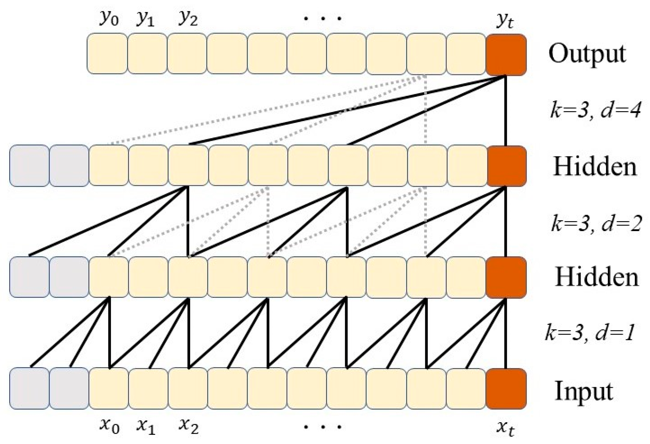
TCN uses causal convolution to restrict the direction of information transfer. Causal convolution is a strictly time-constrained model that ensures the current output is only related to historical data through one-sided padding, avoiding symmetric operations of the convolution kernel. Additionally, each convolutional layer uses dilated convolution to expand the receptive field, as shown in Figure 5. Dilated convolution allows the filter to cover an area larger than its length by skipping certain inputs, enhancing the model’s ability to extract features over long time scales. The mathematical form of dilated convolution is shown in Equation (19).

$$\begin{array}{c}F\left(s\right)=(x \ast d)f\left(s\right)={\displaystyle \sum _{i=0}^{k-1}}f\left(i\right)·x_{s-d·i}\end{array}$$

(19)

where s is the input sequence information, d is the dilation coefficient, k is the filter size, and s − d·i is the direction of the formal sequence.

Combining TCN and GRU leverages the strengths of both models: TCN aids GRU in better capturing global information, while parameter sharing and sparse connection structure in TCN help manage the size of parameters. The TCN-GRU model effectively enhances the efficiency and performance of time series data processing, improving the accuracy of wave elevation reconstruction. Therefore, a three-channel TCN-GRU model is used to simultaneously perform wave elevation reconstruction and dynamic deviation compensation. In this model, the TCN has a filter size of 3 and 16 filters. The number of hidden units in the two-layer GRU is 128 and 64, respectively. The output layer is a fully connected layer with a dimension of 1, producing the wave elevation at the buoy’s initial position.

3. Experiments and Results

3.1. Numerical Simulation

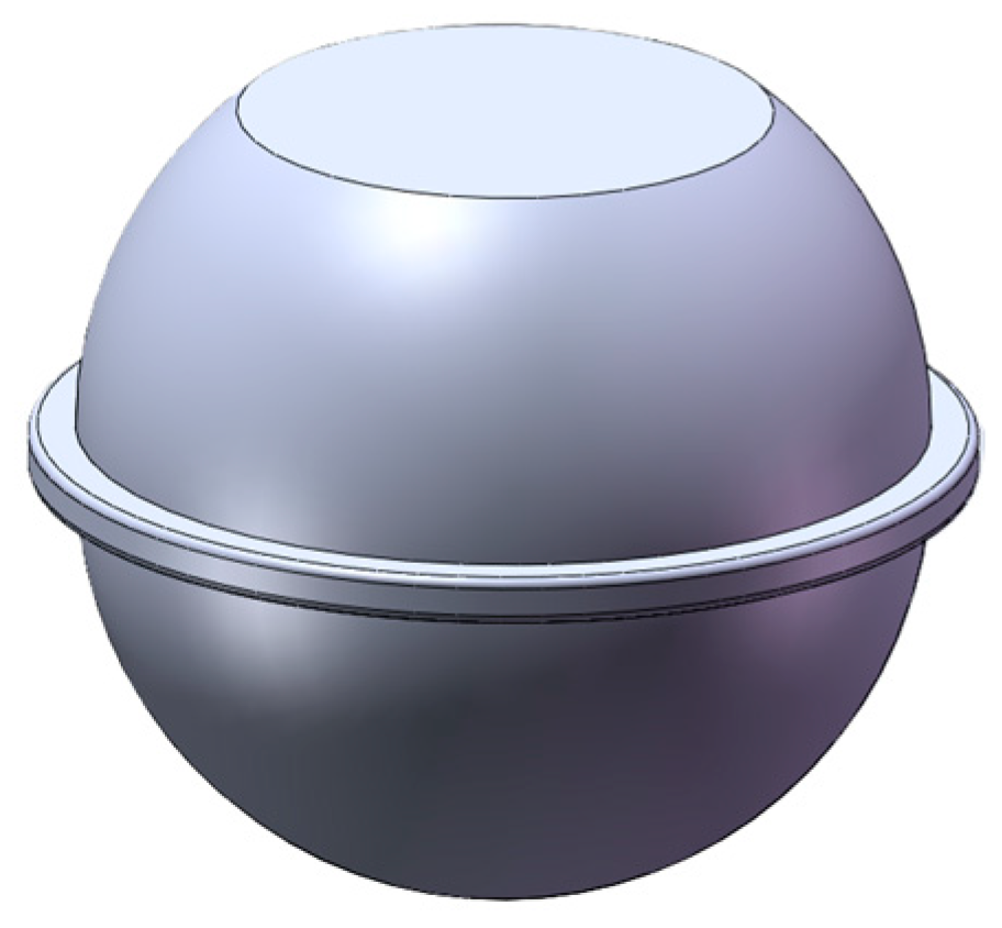
To evaluate the proposed method, experiments were conducted using a wave buoy model with a scale ratio of 10. Numerical simulations were performed under various wave conditions, during which the buoy motion and the wave elevation at different spatial locations were recorded. The measured buoy motion time series were subsequently used for wave elevation reconstruction, and the effects of both static and dynamic deviations on the reconstruction accuracy were analyzed. The buoy model is presented in Figure 6, and the main parameters are listed in

Table 2. Size and parameters of the buoy under simulation.

	Hull Diameter (m)	Weight (kg)	Draught (m)	Scale
Full Scale	0.98	220	0.462	-
Model	0.098	0.216	0.046	10

.

Grids of the numerical tank and the buoy model are shown in Figure 7. To make adequate fluid flow, the inlet of the numerical tank was set at 10 times the hull diameter from the buoy, and the outlet was set at 20 times the hull diameter from the buoy. An overset mesh technique was employed, consisting of a background mesh and a body-fitted volume mesh around the buoy. Local mesh refinement was applied in the vicinity of the free surface using an adaptive mesh refinement (AMR) strategy. The wave direction aligned along the positive X-axis in the global coordinate system.

In computational fluid dynamics (CFD) simulations, a grid independence verification was conducted [27]. The results of the hydrodynamic resistance coefficient for three different grid densities in still water are presented in

Table 3. Results of mesh independence analysis.

Case	Current	Mesh Quantity	Resistance Coefficient	Relative Difference
Sparse	0.05 m/s	1.19 million	0.09201	-
Medium		1.59 million	0.09226	0.27%
Dense		2.23 million	0.09307	1.15%

.

From the independence verification, it can be seen that with the increase in grids, the resistance coefficient does not change significantly. This indicates that when the number of grids reaches 1.59 million, further increasing the grid density does not significantly affect the numerical results. Considering both computational accuracy and cost, subsequent simulations were conducted using a medium grid density of 1.59 million.

Numerical simulations were conducted under irregular wave conditions, and four representative cases were designed based on different sea states; each case corresponds to specific significant wave heights and peak periods. For consistency between the model scale and the full-scale sea state, all wave conditions used in the simulations were derived through Froude similarity. The resulting wave parameters implemented in the numerical model are summarized in

Table 4. Irregular wave parameters.

	Sea State	Significant Wave Height (m)	Peak Period (s)	Wave Spectrum
Case 1	1	0.01	1.265	Pierson-Moskowitz
Case 2	2	0.05	1.613
Case 3	3	0.125	1.938
Case 4	4	0.25	2.277

.

Referring to the 6-DOF motion definition for ships, it was assumed that the buoy was in still water heading along the positive X-axis in the global coordinate system. Affected by a single-flow-direction wave, the buoy primarily exhibits heave, pitch, and surge. In still water, the center of mass of the buoy coincides with the origin of the coordinate system, located directly above the anchor point at the free surface. Therefore, the initial position of the buoy was set at $X=0$.

In the static deviation compensation, multiple wave probes were deployed to investigate how different horizontal deviations affect compensation accuracy. In full-scale conditions, probes were arranged at 1-m intervals along the wave propagation direction, covering positions from $X=0$ to $X=5 \mathrm{m}$. To minimize the hydrodynamic influence of the buoy on the measured wave elevation, all probes were positioned at a lateral offset equal to three times the buoy diameter along the Y-axis. The overall probe arrangement is illustrated in Figure 8. Simultaneously, the 3-DOF buoy motions of pitch, heave, and surge were monitored [28,29]. The surge was considered a dynamic deviation, while the distance between the target position and the initial position was regarded as a static deviation. The buoy’s motion and wave elevation series at the initial position were used to train the TCN-GRU network for wave elevation reconstruction and dynamic deviation compensation. The remaining five wave elevation series were used to evaluate the adaptability of the compensation model for different static deviations.

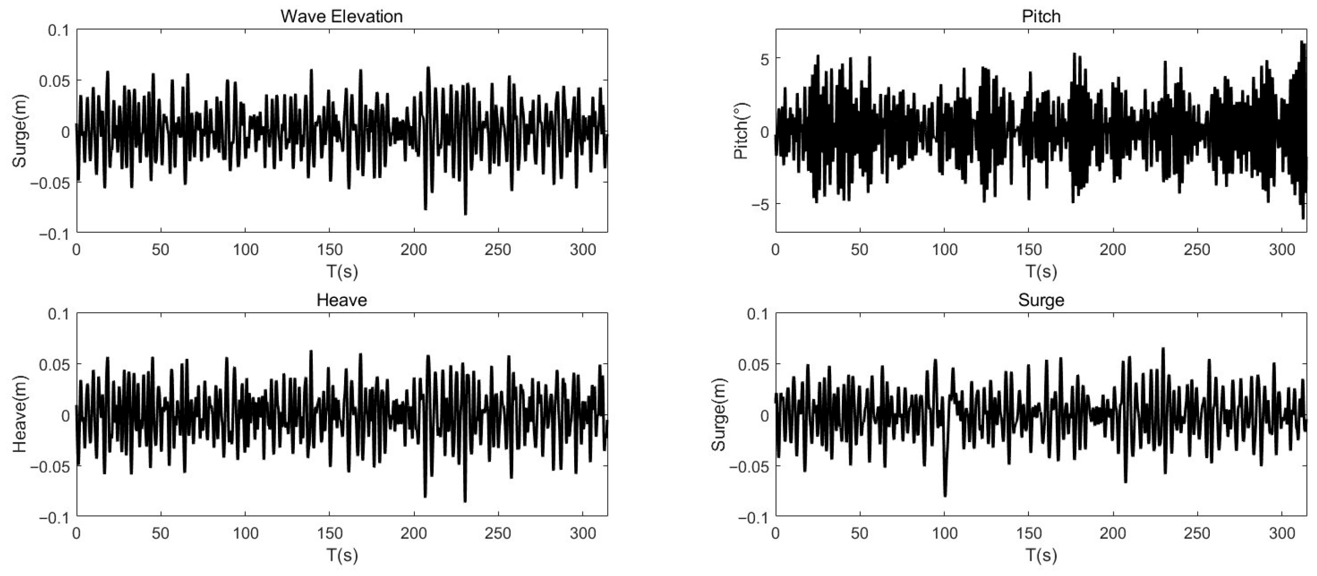
Free surfaces for the four cases are shown in Figure 9. To enable comparison with full-scale offshore conditions, all wave elevation and 3-DOF buoy motion data were converted to full scale using a geometric scale of 10. The restored full-scale wave elevation and buoy motion time series are presented in Figure 10, Figure 11, Figure 12 and Figure 13.

3.2. Dynamic Deviation Compensation

3.2.1. Baseline Performance Under Idealized Conditions

The full-scale wave elevation and 3-DOF buoy motion response for each case were split in time order: the first 80% of each time series was used as the training set, and the remaining 20% was reserved as the test set. The time window for input sequences was set to half of the spectral peak period. The training objective was defined in terms of root mean square error (RMSE) implemented via minimization of mean squared error during optimization, and the trained model performance is reported using RMSE on the held-out test set. Model development and parameter tuning were carried out on the training portion, while final evaluation was performed on the test data.

Training was performed on a GPU-enabled platform using the Adam optimizer in MATLAB R2022b. Models were trained for up to 100 epochs with a batch size of 256. The initial learning rate was 0.005 and was updated with a piecewise schedule, reducing by a factor of 0.5 every 30 epochs to stabilize convergence. To prevent gradient explosion, a gradient threshold of 1 was applied. Input channels were normalized prior to training. Training was run in non-verbose mode and convergence monitored via the recorded loss evolution.

Wave elevation reconstruction and dynamic deviation compensation were performed on the test set. To comprehensively evaluate the performance of the TCN-GRU model in extracting features between buoy motion and wave elevation, comparison experiments were conducted. Both the LSTM and GRU models are widely used deep learning models in time series prediction [30]. Compared to the GRU model, the structure of the LSTM model is more complex. Therefore, GRU, LSTM, and TCN-LSTM were selected in comparison experiments to also validate the effectiveness of the TCN module. In order to comprehensively evaluate the performance of the model in the time domain, mean absolute error (MAE), RMSE, and Spearman’s rank correlation coefficient ($R_s$) were used as indicators. The formulas for the three indicators are shown in Equations (20)–(22).

$$\begin{array}{c}MAE={\displaystyle \frac{1}{n}}{\displaystyle \sum _{i=1}^n}\left|y_i-{\widehat{y}}_i\right|\end{array}$$

(20)

$$\begin{array}{c}RMSE=\sqrt{{\displaystyle \frac{1}{n}}{\displaystyle \sum _{i=1}^n}{\left(y_i-{\widehat{y}}_i\right)}^2}\end{array}$$

(21)

$$\begin{array}{c}{R}_s=1-{\displaystyle \frac{6\sum _{i=1}^n{d}_i^2}{n(n^2-1)}}\end{array}$$

(22)

where $y_i$ is the actual value, ${\widehat{y}}_i$ is the predicted value, and $d_i$ is the rank difference between the predicted and actual values.

Table 5. Time-domain metrics in dynamic deviation compensation.

		LSTM	GRU	TCN-LSTM	TCN-GRU
Case 1	MAE	0.0059	0.0054	0.0032	0.0025
	RMSE	0.0069	0.0067	0.0041	0.0031
	${\mathrm{R}}_{\mathrm{s}}$	0.9639	0.9661	0.9881	0.9940
Case 2	MAE	0.0295	0.0286	0.0243	0.0237
	RMSE	0.0366	0.0352	0.0316	0.0309
	${\mathrm{R}}_{\mathrm{s}}$	0.9566	0.9591	0.9796	0.9765
Case 3	MAE	0.0646	0.0617	0.0544	0.0519
	RMSE	0.0914	0.0844	0.0753	0.0711
	${\mathrm{R}}_{\mathrm{s}}$	0.9618	0.9679	0.9765	0.9829
Case 4	MAE	0.1359	0.1210	0.0875	0.0859
	RMSE	0.1872	0.1792	0.1247	0.1203
	${\mathrm{R}}_{\mathrm{s}}$	0.9679	0.9709	0.9852	0.9862
Model Size		116.5 k	87.2 k	126.3 k	92.4 k

shows the time-domain metrics for the four cases and the optimal results are indicated in bold.

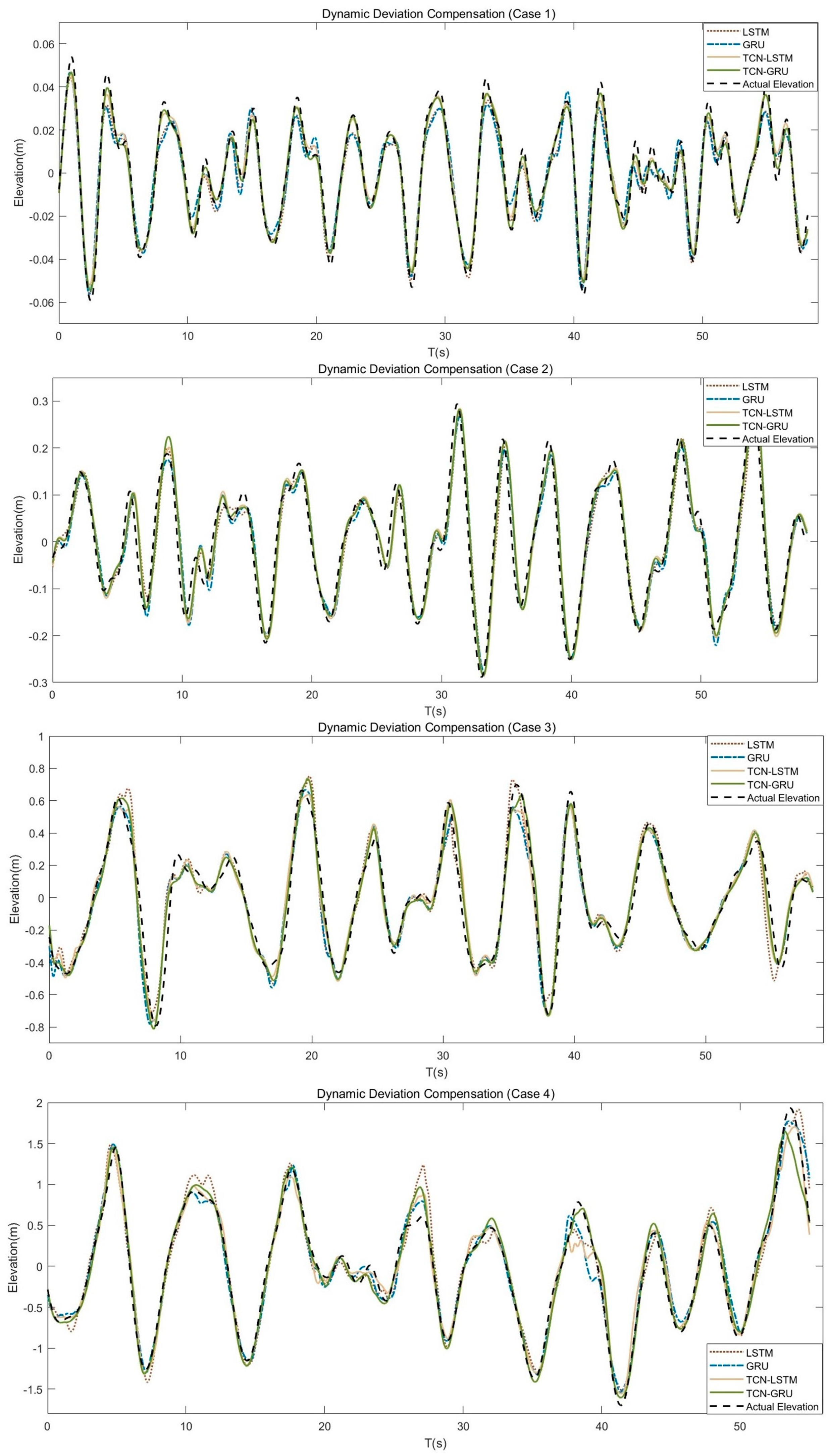
The introduction of the TCN module leads to a consistent and significant improvement in dynamic deviation compensation across all four test cases. Compared with the LSTM and GRU models, the TCN-enhanced networks achieve substantially lower MAE and RMSE values, together with modest but consistent increases in the $R_s$. In Case 1, the MAE and RMSE are reduced by approximately 55–58% relative to the LSTM model and by about 53–54% relative to the GRU model. In Cases 2–4, although the reduction magnitudes are smaller, the TCN-based models still exhibit clear advantages, with MAE reductions ranging from approximately 17% to 37% compared with the LSTM baseline, while $R_s$ increases by roughly 2% to 3% in most cases.

A comparison between the two TCN-based models shows that the TCN-GRU configuration generally provides slightly better performance than TCN-LSTM in terms of MAE and RMSE, and achieves comparable or higher $R_s$ in three of the four cases. From the perspective of model complexity, TCN-GRU requires significantly fewer parameters (approximately 92.4 k) than TCN-LSTM (approximately 126.3 k), while delivering equal or superior compensation accuracy. Although the plain GRU model has the smallest number of parameters (approximately 87.2 k), its compensation accuracy is notably lower than that of the TCN-GRU model.

Figure 14 shows the compensation results on test sets in four cases. The results demonstrate that the TCN module effectively enhances the network’s ability to capture the nonlinear and non-stationary characteristics of buoy motion induced by irregular waves. The TCN-GRU model achieves the best balance between accuracy and model complexity, making it well-suited for wave elevation reconstruction and dynamic deviation compensation. The dynamic compensation results obtained using the TCN-GRU model are therefore adopted as the input for the subsequent static deviation compensation analysis.

3.2.2. Sensitivity Analysis for Motion Measurement Errors

In practical applications, buoy motion measurements are inevitably affected by sensor noise, positioning errors, and low-frequency drift, which may degrade the accuracy of wave elevation reconstruction. To quantitatively evaluate the robustness of the proposed wave elevation reconstruction method against buoy motion measurement errors, a sensitivity analysis for measurement noise is conducted in this section.

The buoy motion responses used in the previous experiments were generated by computational fluid dynamics simulations and are therefore ideal and noise-free. Consequently, synthetic measurement errors are introduced only into the test dataset, while the trained reconstruction model remains unchanged. It is assumed that the buoy observation signals are contaminated by static bias, random measurement noise, and low-frequency drift [31]. The generalized displacement vector of the buoy $\tilde{q}\left(t\right)$ as Equation (23).

$$\begin{array}{c}\tilde{q}\left(t\right)=q\left(t\right)+\tilde{b}+\epsilon \left(t\right)+\tilde{d}\left(t\right)\end{array}$$

(23)

In Equation (22), $\tilde{b}={\left[\begin{array}{cc}\begin{array}{cc}{b}_1& b_2\end{array}& \begin{array}{cc}\cdots & b_n\end{array}\end{array}\right]}^T$ represents the static bias, which accounts for constant offsets caused by sensor zero drift or installation errors. The term $\epsilon \left(t\right)~\mathcal{N}(0, {\sigma }^2\mathrm{I})$ denotes Gaussian measurement noise, where $\sigma$ is the noise intensity, and $\mathrm{I}$ is the identity matrix. The low-frequency drift term $\tilde{d}\left(t_k\right)$ is introduced to simulate slowly varying deviations arising from accumulated positioning errors or low-frequency environmental disturbances. The low-frequency drift is modeled as a random walk process, as expressed in Equation (24).

$$\begin{array}{c}\tilde{d}\left(t_k\right)=\tilde{d}\left(t_{k-1}\right)+\xi \left(t_k\right), \xi \left(t_k\right)~N\left(0, {\sigma }_d^2\mathrm{I}\right)\end{array}$$

(24)

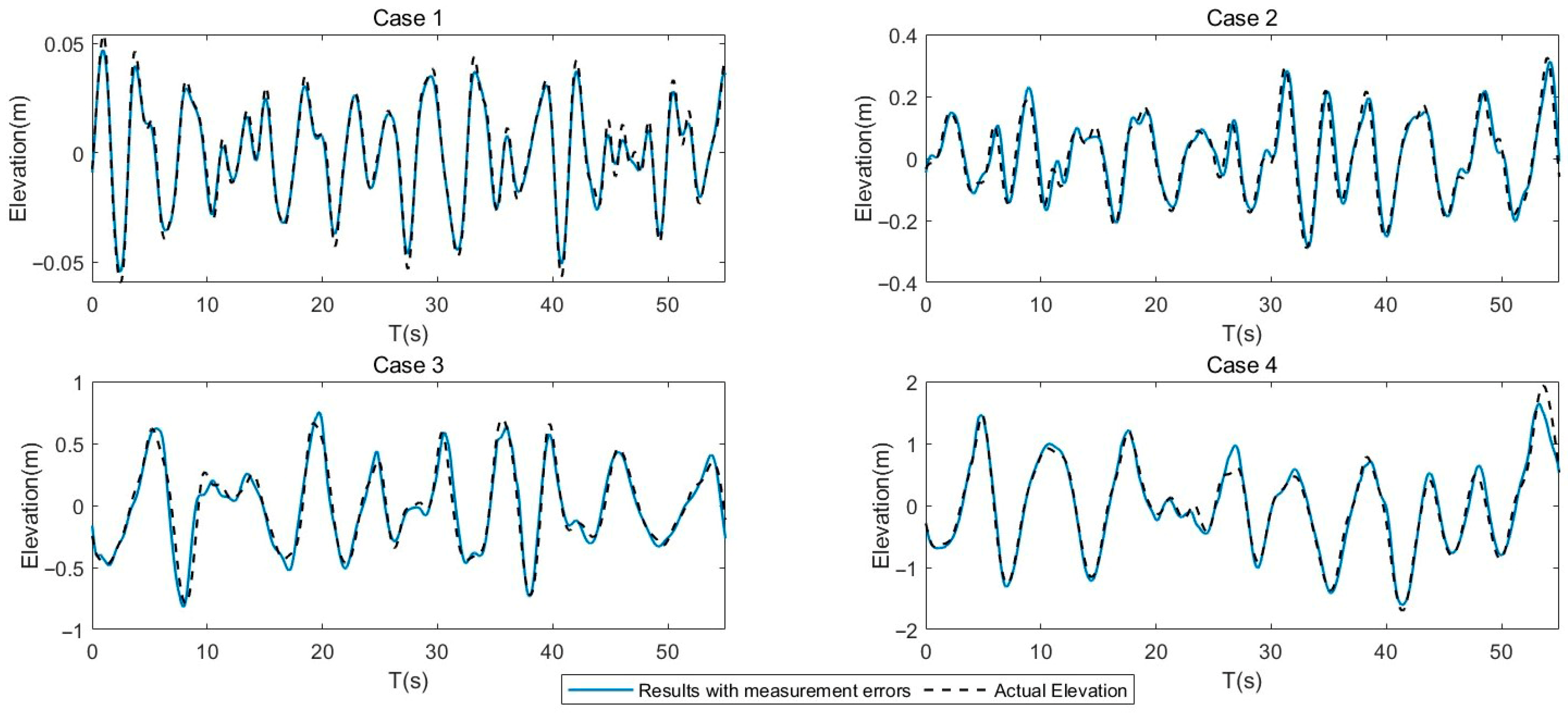
The buoy motion signals contaminated by measurement errors are then fed into the TCN-GRU model to reconstruct the wave elevation at the fixed reference position. The reconstructed results obtained from error-contaminated inputs are compared with those obtained from clean inputs under the same four wave cases, enabling a direct assessment of the influence of buoy motion measurement errors on reconstruction accuracy. The dynamic deviation compensation results and the corresponding error evaluation metrics for the four cases under measurement error conditions are presented in Figure 15 and

Table 6. Time-domain metrics with measurement errors.

	Case 1	Case 2	Case 3	Case 4
MAE	0.0105	0.0308	0.0557	0.0863
RMSE	0.0112	0.0398	0.0777	0.1219
${\mathrm{R}}_{\mathrm{s}}$	0.9891	0.9562	0.9726	0.9859

.

The results indicate that buoy motion measurement errors cause a moderate degradation in reconstruction accuracy across all four wave cases. Compared with the clean-input results, both MAE and RMSE increase when synthetic measurement errors are introduced; however, the overall agreement between the reconstructed and reference wave elevations remains high. In relative terms, the MAE increases by 320.0%, 30.0%, 7.3%, and 0.5% for Case 1 to Case 4, respectively. This trend indicates that the relative impact of measurement errors is most pronounced under mild sea conditions (Case 1), where the wave amplitude is small, and the signal-to-noise ratio is consequently low.

Despite these degradations, the Spearman rank correlation coefficients remain above 0.95 for all cases, demonstrating that the proposed TCN–GRU-based framework effectively preserves the temporal evolution and phase structure of the wave elevation under realistic measurement perturbations. Overall, these quantitative results demonstrate that the proposed wave elevation reconstruction and dynamic deviation compensation method exhibits satisfactory robustness in absolute terms for the tested conditions, while also highlighting an increased sensitivity in low-amplitude wave regimes, where careful sensor calibration and noise mitigation become particularly critical.

3.2.3. Sensitivity Analysis for Wave Propagation Direction Uncertainty

In realistic sea states, the instantaneous propagation direction fluctuates around a dominant direction. To assess the robustness of the proposed reconstruction and dynamic deviation compensation framework to such directional uncertainty, we model the directional variability of the incoming waves and propagate it to the buoy motion inputs used for testing. The two-dimensional wave spectrum is represented as the product of a frequency spectrum and a normalized directional spreading function in Equation (25) [32].

$$\begin{array}{c}{S}_D\left(f,\theta \right)=S_w\left(f\right)D_n\left(\theta -{\theta }_0\right)\end{array}$$

(25)

where $S_w\left(f\right)$ is the wave spectrum, ${\theta }_0$ denotes the dominant incident direction, and $D_n$ is a normalized directional spreading function satisfying ${\int }_{-\pi }^{\pi }{D}_n\left(\varphi \right)d\varphi =1$. In this section, we adopt a commonly used parametric form for the directional spreading in Equation (26).

$$\begin{array}{c}{D}_n\left(\mathsf{\Delta }\theta \right)=C_s{\cos }^{2s}\left({\displaystyle \frac{\mathsf{\Delta }\theta }{2}}\right), \mathsf{\Delta }\theta \in \left[-\pi , \pi \right]\end{array}$$

(26)

where $\mathsf{\Delta }\theta$ is the angular deviation from the dominant direction, $s\ge 0$ is the spreading parameter controlling the angular concentration, and $C_s$ is a normalization constant chosen such that $D_n$ integrates to unity. Based on the prescribed directional spreading function, a continuous angular deviation time series $\mathsf{\Delta }\theta \left(t\right)$, as shown in Figure 16, is constructed whose length matches that of the test dataset. Larger significant wave heights tend to be associated with more directionally concentrated wave fields. The resulting $\mathsf{\Delta }\theta \left(t\right)$ therefore represents a physically plausible realization of continuous wave direction variability consistent with the assumed directional spectrum.

The influence of wave direction uncertainty on buoy motion is introduced by mapping the continuous angular deviation $\mathsf{\Delta }\theta \left(t\right)$ onto the original inputs. Under the assumption of small angular deviations, the effect of a change in incident direction can be approximated through a geometric projection of the horizontal and angular motion components in Equation (27), which corresponds to a first-order approximation of the rotation of the motion components with respect to the dominant direction [33].

$$\begin{array}{c}{q_{xy}}^{\left(\mathsf{\Delta }\theta \right)}\left(t\right)\approx q_{xy}\left(\mathrm{t}\right)cos\mathsf{\Delta }\theta \left(t\right)\end{array}$$

(27)

The heave response is primarily associated with vertical wave-induced motion; it is assumed to be weakly dependent on the incident direction for small angular deviations and is therefore retained unchanged in analysis [34].

Figure 17 presents the dynamic deviation compensation results under continuous wave propagation direction uncertainty. Under the directional spreading constraint, the instantaneous wave direction fluctuates slowly and remains within a limited angular range around the dominant direction. This effect becomes more pronounced for moderate to high sea states, in which wave energy is more directionally concentrated, and deviations from the principal direction are statistically less significant. As a result, the induced variations in the surge and pitch responses are relatively small, while the heave response remains essentially unaffected.

Despite the presence of continuous directional variability, the wave elevation reconstruction accuracy shows no significant degradation within the considered time window and angular deviation range when compared with the ideal unidirectional case. Consequently, the proposed reconstruction and dynamic deviation compensation framework exhibits strong robustness to realistic, slowly varying wave direction uncertainty, supporting its applicability in practical sea conditions dominated by a prevailing wave direction.

3.3. Static Deviation Compensation

The compensation for static deviation is based on the results of dynamic deviation compensation. Figure 18 shows the wave elevation series at different positions in irregular waves. Wave elevations at the six positions exhibit general consistency, with the waves propagating from $X=-5 \mathrm{m}$ to $X=0$. During propagation, the wave deformation increases. The larger the static deviation, the greater the waveform deforms. By substituting the deviation values into Equation (17), the number of time steps required for static deviation compensation is calculated. Figure 19 shows the number of forecast durations needed to compensate for static deviation in the four cases.

In this section, time series prediction models are used for static deviation compensation. The autoregressive model and neural network models are selected to compensate for static deviations in four cases on the test set. The performance of different models is compared in terms of accuracy and efficiency. The advantages of each model in the task are discussed. An auto-regressive integrated moving average (ARIMA) model, which includes autoregressive terms p, differencing terms d, and moving average terms q, can be expressed as Equation (28) [35]. When the ARIMA model is used for multi-step prediction, the result of each prediction will be used as input for the next prediction.

$$\begin{array}{c}{∆}^d{y}_t={ϵ}_t+{∆}^d{\displaystyle \sum _{i=1}^p}{r}_i{y}_{t-i}+{\displaystyle \sum _{i=1}^q}{\theta }_i{ϵ}_{t-i}\end{array}$$

(28)

where $r_i$ and ${\theta }_i$ are the coefficients for the autoregressive part and moving average part, respectively, ${ϵ}_t$ is the white noise error term, $y_t$ is the time series, and ${∆}^d$ is the differencing operator.

Referring to the comparison results of the reconstruction models in the previous section, GRU models are selected in the model comparison experiments. Multi-step predictions by time series forecasting models are achieved through multiple recursive single-step predictions. As shown in Equation (29), the result ${\widehat{y}}_{t+1}$ at time step $t$ is used as the input for step $t+1$. The process will be repeated until the prediction duration $T$ are reached.

$$\begin{array}{c}{\widehat{y}}_{t+k}=f\left(x_{t+k-1},\dots ,{\widehat{y}}_{t+k-1}\right), for k=1, 2, \dots , T\end{array}$$

(29)

For each of the four cases, the static deviation reconstruction used the corresponding dynamic deviation compensation results as inputs. The network models were trained using the wave elevation at the initial reference ($X=0$) from the training dataset. The compensated wave elevations predicted by the three models were then compared against the reference samples at five downstream target positions ranging from $X=-1 \mathrm{m}$ to $X=-5 \mathrm{m}$. The reconstruction results for all four cases at five target positions are presented in Figure 20 and Figure 21.

4. Discussion

To comprehensively evaluate the proposed wave reconstruction and deviation compensation method, a systematic analysis in both time and frequency domains is conducted. The time-domain analysis focuses on quantifying the overall error magnitude and correlation, while the frequency-domain analysis aims to reveal how the reconstruction errors are distributed across different frequency bands, thereby assessing the reliability and limitations of the method in both the dominant energy band and the higher-frequency range.

4.1. Error Evaluation in the Time Domain

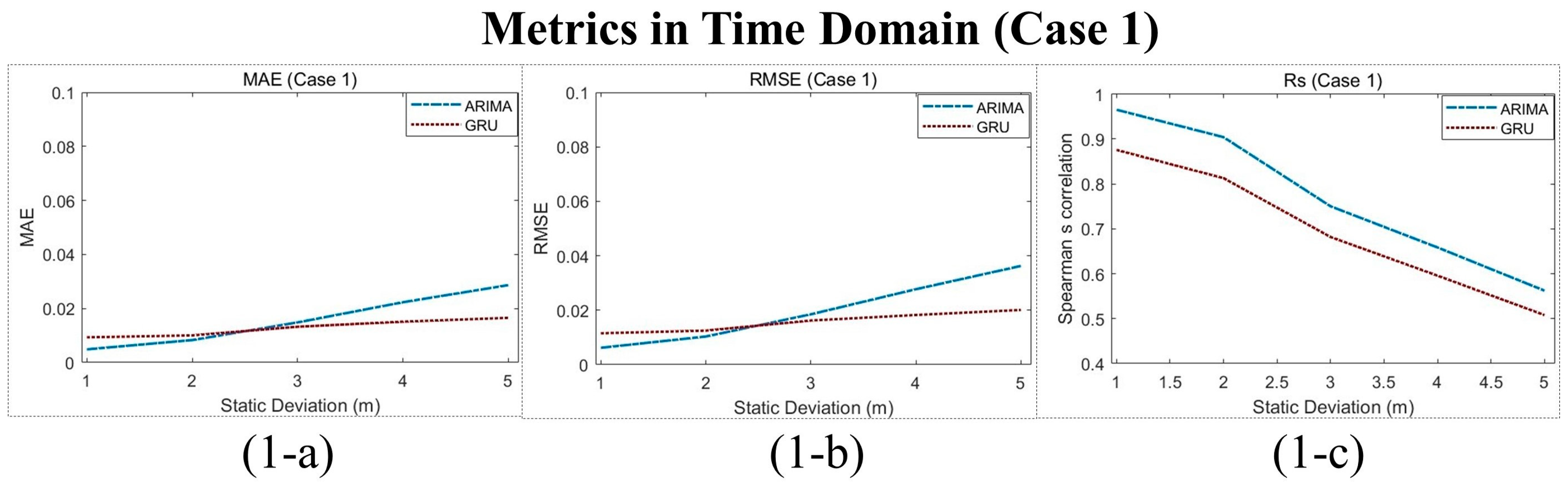
The time-domain evaluation results of the reconstruction errors under four different operating conditions are shown in Figure 22, Figure 23, Figure 24 and Figure 25. The absolute errors generally increase from Case 1 to Case 4 due to the increase in significant wave height, which amplifies the magnitude of reconstruction errors. The variation of $R_s$ exhibits a different and more insightful pattern. For higher sea states, $R_s$ remains relatively high over a wide range of static deviations, particularly for the ARIMA model. This behavior can be attributed to the increase in peak period under severe sea conditions, which reduces the effective prediction time corresponding to a given spatial deviation. As a result, although the absolute reconstruction error increases, the temporal structure and phase evolution of the wave elevation are better preserved, leading to higher rank correlation between the reconstructed and actual waves [36,37].

A comparative analysis of the ARIMA and GRU models demonstrates that ARIMA consistently provides more stable performance across all sea states, especially under medium to large static deviations. Increasing static deviation leads to systematic amplitude error amplification for both ARIMA and GRU; however, the growth characteristics differ markedly. GRU generally exhibits smaller MAE and RMSE at short compensation distances, but these advantages diminish rapidly as deviation increases, with relative error growth often exceeding 150% in moderate sea states. In contrast, ARIMA shows a more gradual increase in normalized MAE and RMSE, typically remaining within 10–15% of significant wave height at large deviations for energetic conditions, indicating better control of long-horizon error accumulation.

This difference in amplitude-error behavior is closely reflected in the evolution of temporal accuracy. While GRU’s rolling multi-step prediction strategy results in sharp declines in $R_s$ as compensation distance increases, ARIMA maintains high rank correlation in higher sea states (e.g., $R_s\gtrsim 90\mathrm{\%}$ at 5 m deviation in Case 4), demonstrating superior preservation of phase and temporal ordering even when MAE and RMSE increase. Together, these MAE/RMSE and $R_s$ trends indicate that, while the GRU model occasionally achieves lower MAE and RMSE at small deviations, the rolling multi-step prediction strategy leads to rapid error accumulation as the compensation distance increases, causing a pronounced degradation in $R_s$. This effect is particularly evident in higher sea states, where long-range temporal dependencies become more critical. As sea states intensify, the wave spectrum becomes increasingly dominated by low-frequency components, which are well captured by linear autoregressive models. Consequently, ARIMA maintains better trend and phase consistency over extended prediction horizons. These results indicate that, for static deviation compensation involving variable prediction steps and wave-dominated signals, ARIMA offers superior stability and practical reliability compared to rolling GRU-based approaches. Compared with neural network-based methods such as GRU, ARIMA offers a notable practical advantage in that it does not require offline pre-training, thereby simplifying model deployment and reducing dependence on large historical training datasets [38].

These results demonstrate that, although both methods exhibit error amplification with increasing compensation distance, ARIMA better preserves the temporal structure and phase consistency of the reconstructed wave elevation, particularly under energetic sea conditions. More critically from an operational standpoint, ARIMA offers significant practical advantages: it is computationally lightweight, can be effectively fitted using short data windows, and requires no offline pre-training. These attributes simplify deployment in real-world offshore monitoring systems and reduce reliance on extensive historical datasets and substantial computational resources. For static deviation compensation tasks involving variable prediction horizons and predominantly wave-driven signals, ARIMA thus represents a robust and readily deployable alternative to rolling-window GRU-based approaches.

4.2. Error Evaluation in Frequency Domain

Based on the time-domain analysis presented above, the ARIMA model demonstrates superior overall accuracy and applicability for static deviation compensation compared with the neural networks. The Welch power spectral density (PSD) estimation method is used to analyze the PSD and cross-spectra of the reconstructed and actual wave elevation time series [39]. Let the actual wave elevation at a given location be denoted as $y\left(n\right)$, and the reconstructed elevation be $\widehat{y}\left(n\right)$. A window function $w\left(n\right)$ of length L is applied to the series, with an overlap of D samples between adjacent segments. Equations (30) and (31) are the wave series after the discrete Fourier transform (DFT).

$$\begin{array}{c}{Y}_m\left(k\right)={\displaystyle \sum _{n=0}^{L-1}}y\left[n+m\left(L-D\right)\right]w\left(n\right)e^{-{\displaystyle \frac{j2\pi kn}{L}}}\end{array}$$

(30)

$$\begin{array}{c}{\widehat{Y}}_m\left(k\right)={\displaystyle \sum _{n=0}^{L-1}}\widehat{y}\left[n+m\left(L-D\right)\right]w\left(n\right)e^{-{\displaystyle \frac{j2\pi kn}{L}}}\end{array}$$

(31)

Cross-spectral analysis is performed between the actual and reconstructed wave elevation sequences. The auto-PSD and cross-PSD estimates of $y\left(n\right)$ and $\widehat{y}\left(n\right)$ are obtained from Equations (32)–(34).

$$\begin{array}{c}{S}_{yy}\left(f_k\right)={\displaystyle \frac{1}{M{f}_s{\sum }_0^{L-1}{w}^2\left(n\right)}}{\displaystyle \sum _{m=0}^{M-1}}{\left|{\displaystyle \sum _{n=0}^{L-1}}{y}_m\left(n\right)e^{-{\displaystyle \frac{j2\pi kn}{L}}}\right|}^2\end{array}$$

(32)

$$\begin{array}{c}{S}_{\widehat{y}\widehat{y}}\left(f_k\right)={\displaystyle \frac{1}{M{f}_s{\sum }_0^{L-1}{w}^2\left(n\right)}}{\displaystyle \sum _{m=0}^{M-1}}{\left|{\displaystyle \sum _{n=0}^{L-1}}{\widehat{y}}_m\left(n\right)e^{-{\displaystyle \frac{j2\pi kn}{L}}}\right|}^2\end{array}$$

(33)

$$\begin{array}{c}{S}_{y\widehat{y}}\left(f_k\right)={\displaystyle \frac{1}{M{f}_s{\sum }_0^{L-1}{w}^2\left(n\right)}}{\displaystyle \sum _{m=0}^{M-1}}{Y}_m\left(k\right){{\widehat{Y}}^{\mathrm{*}}}_m\left(k\right)\end{array}$$

(34)

where ${{\widehat{Y}}^{*}}_m\left(k\right)$ denotes the complex conjugate of the reconstructed elevation spectrum. $f_s$ is the sampling frequency, M is the total number of segments, and $f_k=k{f}_s/L$ denotes the discrete frequency corresponding to the k-th frequency bin in the FFT output.

Based on the above, the coherence function between the actual and reconstructed elevations is defined as Equation (35) [40].

$$\begin{array}{c}{\gamma }_{y\widehat{y}}^2\left(f_k\right)={\displaystyle \frac{{\left|S_{y\widehat{y}}\left(f_k\right)\right|}^2}{S_{yy}\left(f_k\right)S_{\widehat{y}\widehat{y}}\left(f_k\right)}}\end{array}$$

(35)

The squared coherence ${\gamma }_{y\widehat{y}}^2$ is used to quantify the linear correlation between the reconstructed wave elevation time series and the actual wave elevation at each frequency. A coherence value close to unity indicates that the reconstructed wave preserves the amplitude and phase characteristics of the actual wave at the corresponding frequency. Conversely, a coherence value approaching zero implies weak linear correlation in that frequency band, where the reconstructed wave is mainly dominated by noise or prediction errors.

Figure 26 shows the reference wave spectral densities of the four cases derived from the Pierson–Moskowitz spectrum. It can be observed that the dominant wave energy is concentrated within the frequency range of 0.01–0.5 Hz. Even though the four cases share similar frequency ranges, the spectral energy distribution naturally spans a range of wavelengths rather than a single value. The power spectral density confirms that the simulations represent broadband irregular waves, for which changing the spectral parameters would directly alter the effective wavelength distribution. Accordingly, the frequency-domain performance evaluation in this section is focused on this low-frequency band.

For each case, the coherence functions between the ARIMA-corrected reconstructed wave elevations and the corresponding actual wave elevations were computed under different static deviations. The coherence results over the full frequency range and within the dominant frequency band are shown in Figure 27, Figure 28, Figure 29 and Figure 30. As illustrated by the coherence curves, all cases exhibit pronounced coherence peaks in the vicinity of the dominant wave frequency, with coherence values approaching unity. This indicates that the ARIMA-based static deviation compensation is capable of accurately reconstructing the principal dynamic characteristics of the wave within the main energy band. These observations are consistent with the time-domain error analysis presented earlier and further confirm the effectiveness of the proposed compensation methods for low-frequency-dominated wave reconstruction tasks. With increasing frequency, the coherence gradually decreases in the range of approximately 0.15–0.5 Hz and drops to relatively low levels at higher frequencies. It suggests a significant reduction in linear correlation between the reconstructed and actual wave elevations at high frequencies.

It is also worth noting that the reconstruction inevitably introduces additional high-frequency components superimposed on the true wave elevation time series. In frequency-domain results, these high-frequency contributions generally exhibit very low coherence (typically below 0.3), although occasional narrow-band frequencies with somewhat higher coherence are observed. Such behavior mainly arises from random phase alignment or noise interference in low-energy high-frequency bands and does not indicate a stable or physically meaningful reconstruction capability [41]. Practically, this has two consequences: (1) parameters and phenomena governed by the dominant spectral band (e.g., significant wave height and peak period) are largely unaffected because coherence near the spectral peak remains near unity; (2) applications that require faithful high-frequency detail (for example short-crested wave detection, breaking crest resolution, or high-frequency structural load estimation) may be degraded by the introduced noise. In engineering practice, appropriate low-pass filters or spectral masks can be applied to suppress irrelevant high-frequency components. Overall, while high-frequency noise is an unavoidable by-product of the reconstruction, it does not materially reduce the method’s effectiveness for recovering the dominant wave components that are most relevant to offshore monitoring and operational decision making.

A further comparison of the coherence results under different static deviations reveals that, although the overall trends of the coherence curves remain similar as the static deviation increases from 1 m to 5 m, the peak coherence values within the dominant frequency band exhibit a gradual decline with increasing deviation, while the dominant frequency location remains essentially unchanged. Meanwhile, the coherence within the low-frequency main energy band generally remains at a relatively high level, indicating that the ARIMA-based static deviation compensation retains a certain degree of robustness against varying static deviations.

5. Conclusions

The primary objective of this study is to achieve accurate reconstruction of wave elevation time series at a fixed spatial position using measurements from drifting wave buoys. To address this challenge, a fixed-position wave-elevation reconstruction framework is proposed that (1) employs a TCN–GRU hybrid network for wave elevation reconstruction and dynamic deviation compensation to remove motion-induced effects, and (2) applies a physics-informed static-deviation compensation strategy that maps spatial offsets into temporal misalignment, followed by time series prediction to recover the incident wavefront.

Extensive numerical experiments with four representative sea states demonstrate the effectiveness of the combined approach. Reconstruction errors in higher-energy seas typically remain within approximately 10–15% even at large static deviations. Frequency domain analysis shows that the static-compensation strategy preserves near-unity coherence at the spectral peak, while coherence typically falls below about 0.3 at higher frequencies, indicating that the method reliably reconstructs the dominant wave components, although limited high-frequency noise may be introduced. Sensitivity analyses further show that the proposed method remains robust to realistic buoy measurement errors and slowly varying wave-direction uncertainty, with reconstruction accuracy only moderately affected.

Despite these strengths, the method has limitations under conditions of strong spatial inhomogeneity or when faithful high-frequency reconstruction is required. First, large bathymetric gradients, strong mean currents, or rapidly varying directional seas can violate the local-invariance assumptions underlying the static compensation. Then, these high-frequency components, which typically exhibit low coherence, may degrade performance in applications requiring accurate high-frequency details, such as breaking-crest detection or high-frequency structural-load estimation. In engineering practice, these effects can be mitigated by applying modest low-pass or spectral masking to suppress incoherent high-frequency content. Future work will focus on further enhancing model adaptability by incorporating advanced learning strategies or hybrid physics–data-driven approaches, with the aim of improving long-horizon compensation accuracy under severe sea states.

References

1. Bielicki, S. Prediction Of Ship Motions In Irregular Waves Based On Response Amplitude Operators Evaluated Experimentally In Noise Waves. Pol. Marit. Res. 2021, 28, 16–27. [Google Scholar] [CrossRef]
2. Cademartori, G.; Oneto, L.; Valdenazzi, F.; Coraddu, A.; Gambino, A.; Anguita, D. A review on ship motions and quiescent periods prediction models. Ocean Eng. 2023, 280, 114822. [Google Scholar] [CrossRef]
3. Aoki, Y.; Sasaki, K.; Nakamura, R.; Ishibashi, K.; Yamamoto, K.; Inagaki, N.; Shibayama, T. Laboratory study on effect of vegetation in reducing wave overtopping under wind effect. Ocean Eng. 2024, 311, 118984. [Google Scholar] [CrossRef]
4. Li, J.; Zhang, H.; Hou, P.; Fu, B.; Zheng, G. Mapping the bathymetry of shallow coastal water using single-frame fine-resolution optical remote sensing imagery. Acta Oceanol. Sin. 2016, 35, 60–66. [Google Scholar] [CrossRef]
5. Molfetta, M.G.; Bruno, M.F.; Pratola, L.; Rinaldi, A.; Morea, A.; Preziosa, G.; Pasquali, D.; Di Risio, M.; Mossa, M. A Sterescopic System to Measure Water Waves in Laboratories. Remote Sens. 2020, 12, 2288. [Google Scholar] [CrossRef]
6. Tian, X.M.; Song, Y. Machine Learning for Short-Term Prediction of Ship Motion Combined with Wave Input. Appl. Sci. 2023, 13, 5298. [Google Scholar] [CrossRef]
7. Rossi, G.B.; Cannata, A.; Iengo, A.; Migliaccio, M.; Nardone, G.; Piscopo, V.; Zambianchi, E. Measurement of Sea Waves. Sensors 2022, 22, 78. [Google Scholar] [CrossRef]
8. Saetre, C.; Tholo, H.; Hovdenes, J.; Kocbach, J.; Hageberg, A.A.; Klepsvik, I.; Aarnes, O.J.; Furevik, B.R.; Magnusson, A.K. Directional wave measurements from navigational buoys. Ocean Eng. 2023, 268, 113161. [Google Scholar] [CrossRef]
9. Raghukumar, K.; Chang, G.; Spada, F.; Jones, C.; Janssen, T.; Gans, A. Performance Characteristics of “Spotter,” a Newly Developed Real-Time Wave Measurement Buoy. J. Atmos. Ocean. Technol. 2019, 36, 1127–1141. [Google Scholar] [CrossRef]
10. Fisher, A.; Thomson, J.; Schwendeman, M. Rapid deterministic wave prediction using a sparse array of buoys. Ocean Eng. 2021, 228, 108871. [Google Scholar] [CrossRef]
11. Liu, Y.; Li, M.H.; Liu, Y.X.; Wang, Y.F.; Jiang, S.M.; Wang, Y.B.; Tian, L.; Qiao, F.L. Real-time precise measurements of ocean surface waves using GNSS variometric approach. Int. J. Appl. Earth Obs. Geoinf. 2022, 115, 103125. [Google Scholar] [CrossRef]
12. Herbers, T.; Jessen, P.F.; Janssen, T.T.; Colbert, D.B.; Macmahan, J.H. Observing Ocean Surface Waves with GPS-Tracked Buoys. J. Atmos. Ocean. Technol. 2012, 29, 944–959. [Google Scholar] [CrossRef]
13. Saviz Naeini, S.; Snaiki, R. A physics-informed machine learning model for time-dependent wave runup prediction. Ocean Eng. 2024, 295, 116986. [Google Scholar] [CrossRef]
14. Ehlers, S.; Stender, M.; Hoffmann, N. Bridging ocean wave physics and deep learning: Physics-informed neural operators for nonlinear wavefield reconstruction in real-time. Phys. Fluids 2025, 37, 107119. [Google Scholar] [CrossRef]
15. Lv, C.; Song, N.; Nie, J.; Ye, M.; Liang, X.; Jia, D.; Ni, X. Hybrid wave height forecasting via integrated physics-based simulation and data-driven correction with contrastive feature fusion. Appl. Ocean Res. 2025, 162, 104729. [Google Scholar] [CrossRef]
16. Raissi, M.; Perdikaris, P.; Karniadakis, G.E. Physics-informed neural networks: A deep learning framework for solving forward and inverse problems involving nonlinear partial differential equations. J. Comput. Phys. 2019, 378, 686–707. [Google Scholar] [CrossRef]
17. Desouky, M.; Abdelkhalik, O. Wave prediction using wave rider position measurements and NARX network in wave energy conversion. Appl. Ocean Res. 2019, 82, 10–21. [Google Scholar] [CrossRef]
18. Qin, Y.; Huang, L.; Wang, X.; Ma, X.; Duan, W.; Hao, W. Feasibility of Wave Measurement by Using a Sailing Buoy and the Artificial Neural Network Technique. J. Shanghai Jiaotong Univ. 2022, 56, 498–505. [Google Scholar]
19. Nielsen, U.D.; Iwase, K.; Mounet, R.E.G. Comparing machine learning-based sea state estimates by the wave buoy analogy. Appl. Ocean Res. 2024, 149, 104042. [Google Scholar] [CrossRef]
20. Ding, Y.; Taylor, P.H.; Zhao, W.; Dory, J.; Hlophe, T.; Draper, S. Oceanographic wave buoy motion as a 3D-vector field: Spectra, linear components and bound harmonics. Appl. Ocean Res. 2023, 141, 103777. [Google Scholar] [CrossRef]
21. Yayi, L.; Aifeng, T.; Haiming, Z.; Wei, X.; Xiao, X.; Zhenyao, Z. Fast Calibration and Wave Making Method Based on Wave Attenuation Analysis. Res. Explor. Lab. 2020, 39, 25–28. [Google Scholar]
22. Skjelbreia, L.; Hendrickson, J. Fifth order gravity wave theory. Coast. Eng. Proc. 1960, 1, 10. [Google Scholar] [CrossRef]
23. Fenton, J.D. A Fifth-Order Stokes Theory for Steady Waves. J. Waterw. Port Coast. Ocean. Eng. 1985, 111, 216–234. [Google Scholar] [CrossRef]
24. Cho, K.; van Merrienboer, B.; Gulcehre, C.; Bahdanau, D.; Bougares, F.; Schwenk, H.; Bengio, Y. Learning Phrase Representations using RNN Encoder-Decoder for Statistical Machine Translation. arXiv 2014, arXiv:1406.1078. [Google Scholar] [CrossRef]
25. Yu, Y.; Si, X.S.; Hu, C.H.; Zhang, J.X. A Review of Recurrent Neural Networks: LSTM Cells and Network Architectures. Neural Comput. 2019, 31, 1235–1270. [Google Scholar] [CrossRef] [PubMed]
26. Bai, S.; Zico Kolter, J.; Koltun, V. An Empirical Evaluation of Generic Convolutional and Recurrent Networks for Sequence Modeling. arXiv 2018, arXiv:1803.01271. [Google Scholar] [CrossRef]
27. Lee, M.; Park, G.; Park, C.; Kim, C. Improvement of Grid Independence Test for Computational Fluid Dynamics Model of Building Based on Grid Resolution. Adv. Civ. Eng. 2020, 2020, 8827936. [Google Scholar] [CrossRef]
28. Fernandes, A.C.; de Araujo, J.B.; de Almeida, J.; Matos, R. Torpedo anchor installation hydrodynamics. J. Offshore Mech. Arct. Eng. Trans. ASME 2006, 128, 286–293. [Google Scholar] [CrossRef]
29. Li, M.; Wu, R.K.; Wu, B.J.; Yang, Z.H.; Li, G. Hydrodynamic performance and optimization of a pneumatic type spar buoy wave energy converter. Ocean Eng. 2022, 254, 111334. [Google Scholar] [CrossRef]
30. Chung, J.; Gulcehre, C.; Cho, K.; Bengio, Y. Empirical Evaluation of Gated Recurrent Neural Networks on Sequence Modeling. arXiv 2014, arXiv:1412.3555. [Google Scholar] [CrossRef]
31. Ashton, I.G.C.; Johanning, L. On errors in low frequency wave measurements from wave buoys. Ocean Eng. 2015, 95, 11–22. [Google Scholar] [CrossRef]
32. Sanil Kumar, V.; Deo, M.C.; Anand, N.M.; Ashok Kumar, K. Directional spread parameter at intermediate water depth. Ocean Eng. 2000, 27, 889–905. [Google Scholar] [CrossRef]
33. Tucker, M.J. Interpreting directional data from large pitch-roll-heave buoys. Ocean Eng. 1989, 16, 173–192. [Google Scholar] [CrossRef]
34. Barstow, S.; Krogstad, H. General Analysis of Directional Ocean Wave Data from Heave Pitch Roll Buoys. Model. Identif. Control. A Nor. Res. Bull. 1984, 5, 47–70. [Google Scholar] [CrossRef]
35. Tarmanini, C.; Sarma, N.; Gezegin, C.; Ozgonenel, O. Short term load forecasting based on ARIMA and ANN approaches. Energy Rep. 2023, 9, 550–557. [Google Scholar] [CrossRef]
36. Kontopoulou, V.I.; Panagopoulos, A.D.; Kakkos, I.; Matsopoulos, G.K. A Review of ARIMA vs. Machine Learning Approaches for Time Series Forecasting in Data Driven Networks. Future Internet 2023, 15, 255. [Google Scholar] [CrossRef]
37. Zhang, G.P. Time series forecasting using a hybrid ARIMA and neural network model. Neurocomputing 2003, 50, 159–175. [Google Scholar] [CrossRef]
38. Siami-Namini, S.; Siami Namin, A. Forecasting Economics and Financial Time Series: ARIMA vs. LSTM. arXiv 2018, arXiv:1803.06386. [Google Scholar] [CrossRef]
39. Welch, P. The use of fast Fourier transform for the estimation of power spectra: A method based on time averaging over short, modified periodograms. IEEE Trans. Audio Electroacoust. 1967, 15, 70–73. [Google Scholar] [CrossRef]
40. Gardner, W.A. A unifying view of coherence in signal processing. Signal Process. 1992, 29, 113–140. [Google Scholar] [CrossRef]
41. Gujral, H.; Kushwaha, A.K.; Khurana, S. Utilization of Time Series Tools in Life-sciences and Neuroscience. Neurosci. Insights 2020, 15, 1489261083. [Google Scholar] [CrossRef] [PubMed]
Figure 1. Method framework.
Applsci 16 00898 g001
Figure 2. Static and dynamic deviation.
Applsci 16 00898 g002
Figure 3. Architecture of the TCN-GRU: (a) TCN-GRU model; (b) TCN model; (c) GRU model.
Applsci 16 00898 g003
Figure 4. GRU & LSTM units: (a) GRU unit; (b) LSTM unit.
Applsci 16 00898 g004
Figure 5. Dilated convolution.
Applsci 16 00898 g005
Figure 6. Buoy model.
Applsci 16 00898 g006
Figure 7. Computational domain and buoy mesh.
Applsci 16 00898 g007
Figure 8. Wave Elevation Monitoring (In Still Water).
Applsci 16 00898 g008
Figure 9. Free surface of the four cases in numerical simulation: (a) Case 1; (b) Case 2; (c) Case 3; (d) Case 4.
Applsci 16 00898 g009
Figure 10. Wave elevation and buoy motions in Case 1.
Applsci 16 00898 g010
Figure 11. Wave elevation and buoy motions in Case 2.
Applsci 16 00898 g011
Figure 12. Wave elevation and buoy motions in Case 3.
Applsci 16 00898 g012
Figure 13. Wave elevation and buoy motions in Case 4.
Applsci 16 00898 g013
Figure 14. Dynamic deviation compensation in the four Cases.
Applsci 16 00898 g014
Figure 15. Compensation results with measurement errors.
Applsci 16 00898 g015
Figure 16. Angular deviation from the dominant direction.
Applsci 16 00898 g016
Figure 17. Compensation results with angular deviation.
Applsci 16 00898 g017
Figure 18. Wave elevation with different static deviation (Case 4).
Applsci 16 00898 g018
Figure 19. Forecast duration in four cases.
Applsci 16 00898 g019
Figure 20. Static deviations in Case 1 and Case 2.
Applsci 16 00898 g020
Figure 21. Static deviations in Case 3 and Case 4.
Applsci 16 00898 g021
Figure 22. Static deviation compensation in Case 1: (1-a) MAE; (1-b) RMSE; (1-c) Spearman’s correlation.
Applsci 16 00898 g022
Figure 23. Static deviation compensation in Case 2: (2-a) MAE; (2-b) RMSE; (2-c) Spearman’s correlation.
Applsci 16 00898 g023
Figure 24. Static deviation compensation in Case 3: (3-a) MAE; (3-b) RMSE; (3-c) Spearman’s correlation.
Applsci 16 00898 g024
Figure 25. Static deviation compensation in Case 4: (4-a) MAE; (4-b) RMSE; (4-c) Spearman’s correlation.
Applsci 16 00898 g025
Figure 26. P–M spectrum for the four cases.
Applsci 16 00898 g026
Figure 27. Coherence function for Case 1.
Applsci 16 00898 g027
Figure 28. Coherence function for Case 2.
Applsci 16 00898 g028
Figure 29. Coherence function for Case 3.
Applsci 16 00898 g029
Figure 30. Coherence function for Case 4.
Applsci 16 00898 g030