Abstract
The accurate calculation of gear time-varying mesh stiffness is of significant importance for the dynamic modeling of gear systems. Currently, research on calculation methods for helical gear mesh stiffness is relatively limited, with the primary approaches being finite element methods and analytical methods. This paper proposes an optimized helical gear meshing stiffness model. Building upon the slice potential method, this approach comprehensively accounts for the effects of tooth-surface friction and local contact deformation. Results indicate that tooth surface friction causes abrupt changes in meshing stiffness values, while local contact deformation leads to an overall decrease in meshing stiffness values. To validate the application value of the optimized calculation method, the contact line method was replaced with the optimized slice potential energy method for simulating the external sound field of locomotive traction transmission systems. Comparisons with actual measurement data revealed that the sound pressure level data from this study’s meshing stiffness model align more closely with experimental results than those from the contact line method model, with the maximum error decreasing from 5% to 2.2%, effectively enhancing the accuracy of the rapid modeling method.
1. Introduction
The formation of time-varying mesh stiffness originates from the change in deformation of a tooth pair along the meshing line as the meshing position varies, while the meshing position itself is time-dependent. The fluctuation of time-varying mesh stiffness is one of the primary internal excitations in gear transmission systems and may induce undesirable dynamic responses such as vibration and noise [1,2]. Therefore, accurate calculation of gear mesh stiffness has become a crucial foundation for establishing reliable dynamic models of gear systems.
While spur gears serve as a fundamental model, helical gears introduce greater complexity. The inclusion of the helix angle significantly increases the total contact ratio. Furthermore, helical gears possess more intricate time-varying meshing parameters. These factors make calculating TVMS for helical gears considerably more challenging than for their spur gear counterparts.
Numerous methodologies for calculating TVMS have been established and refined. The predominant techniques include the Finite Element Method (FEM) [3,4], the Analytical Method [5,6,7], hybrid approaches combining FEM and analytical solutions [8,9], Empirical Formula Methods [10,11], and approximate algorithms based on ISO standards [12]. Despite this diversity, experimental techniques face significant hurdles in achieving precise direct measurements of mesh stiffness. Therefore, the Finite Element Method and the Analytical Method remain the two principal tools for the accurate computation of gear tooth mesh stiffness [13].
Current research on mesh stiffness calculation methods is predominantly focused on spur gears, with studies on helical gears being relatively limited. Within this context, the Finite Element Method is still a primary means for calculating helical gear TVMS [14]. Dell’Accio and Guessab et al. [15] proposed a polynomial enhancement strategy that improves approximation accuracy while maintaining a low condition number of the stiffness matrix. However, FEM requires the construction of detailed three-dimensional finite element models, which involves considerable computational expense. To balance computational efficiency and accuracy, an analytical approach known as the Slicing Method based on the Principle of Potential Energy has been widely adopted. Extensively validated, this method has proven effective in calculating the mesh stiffness of both helical and spur gears, even under conditions such as misalignment, tooth profile errors, and localized cracks [7,16,17].
On the basis of the classical slice potential energy method, Yang and Chen et al. [18] proposed an improved potential energy method applicable to spur gears. The improvement lies in accounting for the difference between the base circle radius and the tooth root radius, thereby enhancing calculation accuracy. For helical gears, researchers integrated spur gear mesh stiffness theory into the traditional slice method and introduced time-varying inter-tooth effects, leading to the development of new time-varying mesh stiffness calculation methods for helical gears. Wan et al. [19] proposed an improved time-varying mesh stiffness algorithm based on the slice potential energy method. A coupled transverse-torsional dynamic model was adopted to simulate the vibration response of a geared rotor system with cracked teeth. The effects of geometric transmission error (GTE), bearing stiffness, and gear mesh stiffness on the dynamic model were analyzed. Experimental validation was conducted on a test rig, demonstrating close agreement between experimental and simulation results.
Subsequent studies have further extended the applicability and accuracy of these methods: Wu et al. [20] proposed a novel method for evaluating the effect of tooth-surface pitting with curved-bottom characteristics on the time-varying mesh stiffness of helical gears. Li et al. [21] proposed an analytical method based on Hertz contact theory, half-space theory, and the principle of minimum potential energy, enabling accurate calculation of local contact stiffness. Zhao et al. [22] proposed a method based on a modified fractal contact model to calculate mesh stiffness while accounting for friction effects. Li and Chen et al. [23] proposed a method for calculating mesh stiffness that incorporates sliding friction effects based on the Ishikawa model. Regarding the tooth-surface friction coefficient, Marjanovic and Ivkovic et al. [24] defined a tribological research procedure for identifying the dependency of the friction coefficient on sliding velocity and contact pressure. Dai et al. [25] developed an innovative model that simultaneously considers two critical factors: tip relief and variable loading conditions. Flek et al. [26] assessed the applicability of an analytical model by conducting an objective comparison of its results against high-fidelity finite element analysis outcomes. Yu et al. [27] enhanced the traditional slicing principle by distributing parabolic-shaped weighting factors along the tooth width on the sliced segments. This modification accounts for coupling effects, yielding more accurate results in single-tooth-pair stiffness calculations. Hou et al. [28] enhanced the traditional calculation method by incorporating structural coupling and slice-coupling effects between adjacent tooth segments. Their established comprehensive helical gear mesh stiffness model also accounts for the influence of the axial component of the meshing force. Tang et al. [29], based on the potential energy method, proposed a comprehensive mesh stiffness calculation method for spur gears and further developed single-coupling and dual-coupling models to compute the mesh stiffness of helical gear pairs.
In summary, compared to spur gears, the research framework for analytical methods of helical gear mesh stiffness remains significantly underdeveloped. As shown in the preceding literature review, although some scholars have explored the influence of tooth-surface friction and local contact effects on helical gear stiffness calculation, few studies have systematically considered tooth-surface parameters based on the slice potential energy method. While the current slice potential energy method for helical gears demonstrates high accuracy and reliability, its integration of factors such as tooth-surface friction and local contact deformation is still incomplete. To address this research gap, this study incorporates the fundamental mechanism of tooth-surface friction and the deformation logic of contact points into the slice potential energy method. We propose an optimized slicing potential energy method that holistically incorporates these critical factors. By preserving the high reliability and accuracy of the original method while introducing considerations for additional tooth-surface phenomena, the proposed approach yields mesh stiffness values that align more closely with real-world operating conditions than those obtained by the original method. This enhancement ultimately improves the practical application value and fidelity of the method in dynamic analysis and gear design.
2. An Optimized Model for Determining Time-Varying Engagement Stiffness Based on the Slice Potential Energy Method
This section introduces a method for calculating the normal flexibility and meshing stiffness of helical gear tooth surfaces. It combines the energy method and the slicing method while incorporating tooth-surface friction and local contact deformation. Building upon the high accuracy and reliability of the slicing potential energy method, this approach accounts for friction and deformation, resulting in calculation outcomes that align more closely with actual conditions than those from the original method. All theoretical calculations of mesh stiffness in this study are performed using MATLAB [30].
2.1. Method for Determining Engagement Stiffness Based on the Energy Approach and Slicing Method
The slicing potential energy method discretizes the helical gear along its face width into a succession of independent, equally thick cantilever-beam slices, as illustrated in the schematic diagram of the helical gear slice model (Figure 1). Each of these resulting gear slices can be conceptually modeled as a thin spur gear, with each retaining an identical transverse tooth profile to that of the original helical gear.
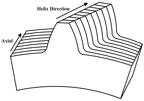
Figure 1.
Schematic Diagram of Helical Gear Cross-Section Model.
In current slice potential energy methods, the total gear meshing potential energy is typically calculated based on bending potential energy , shear potential energy , axial compression potential energy , and Hertz contact potential energy . Among these, Hertz contact potential energy refers to the expression, according to Hertz contact theory, of the relationship between the normal elastic approach deformation and the contact force at the contact point of two elastic bodies in the form of a potential energy function [31]. This study adopts classical assumptions by simplifying the tooth as a cantilever beam fixed on the base circle. Under this simplified premise and based on energy conservation, the bending stiffness , shear stiffness , axial compression stiffness , and Hertz contact stiffness can be derived. Correspondingly, Hertz contact stiffness is defined as the reciprocal of the normal contact deformation induced by a unit contact force when two tooth surfaces undergo local elastic deformation due to contact stress at the contact point during gear meshing [31]. The expressions for , , , and are given as follows:
In the expressions above, denotes the resultant force acting on the meshing teeth at the contact point, represents the radial force, represents the tangential force, is the shear modulus, is Young’s modulus, denotes the area moment of inertia of the gear tooth at a distance from the tooth root, and denotes the cross-sectional area of the gear tooth at a distance from the tooth root. The mathematical expressions for these parameters are given as follows:
Here, and correspond to the tooth width and Poisson’s ratio, respectively. The remaining parameters are shown in Figure 2.
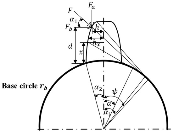
Figure 2.
Tooth-Surface Parameters Diagram.
Based on the parameters in Figure 2 and the geometric characteristics of the involute tooth profile, the parameters , , and in Equation (1) can be expressed as:
By combining Equation (1) with Equations (5)–(9), a formula for bending stiffness expressed in terms of the tooth profile parameters , , and can be derived. To facilitate calculation using angular variables , Equation (10) is substituted into the aforementioned bending stiffness formula. After simplification, the expression for bending meshing stiffness is obtained as follows:
Similarly, the shear engagement stiffness and axial compression stiffness can be expressed as:
By applying the principle of superposition, the total potential energy of the system during gear meshing can be determined:
Among them:
denotes the total equivalent meshing stiffness; subscripts 1 and 2 represent the driving gear and driven gear, respectively.
In addition to tooth deformation, based on the gear body deformation formula derived by Sainsot et al. [6], the partial deformation of the gear body at the contact point under unit load is:
In the equation, and are shown in Figure 3. The coefficients , , , and are approximated by the following polynomials:
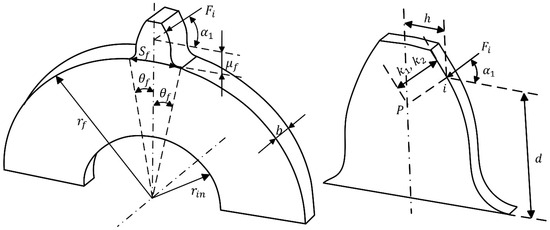
Figure 3.
Wheel Body Deformation Parameters Diagram and Tooth-Surface Parameters Diagram.
In the equation, represents , , , and ; ; and the values of , , , , , and are shown in Table 1.

Table 1.
Coefficient Values in Equation (17).
In summary, the total equivalent meshing stiffness of a single pair of meshing gears can be obtained by superimposing the bending stiffness, shear stiffness, axial compression stiffness, Hertzian contact stiffness of the driving and driven gears, and the equivalent stiffness of the gear body section. The calculation formula is:
Subscripts 1 and 2 denote the driving wheel and driven wheel, respectively.
Based on the slice potential method described above, the meshing stiffness of the gears in Table 2 was calculated. The results are shown in Figure 4. The left diagram illustrates the variation in single-tooth meshing stiffness as the position of the meshing line changes. The right diagram shows the trend of time-varying meshing stiffness as the number of teeth alternates between two and three. The load condition for the calculation results in the figure corresponds to the rated load, i.e., a driven wheel torque of 20,233 Nm. Subsequent comparative calculations of results are also based on the rated load.
Table 2.
Basic parameters of gears.
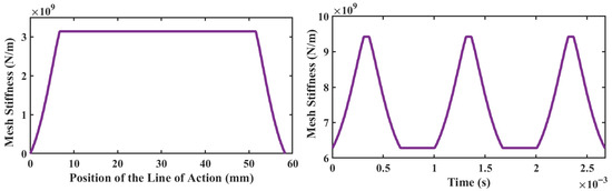
Figure 4.
Engaging stiffness curves obtained using the slice potential method (Left: single-tooth engaging stiffness curve; Right: multi-tooth engaging stiffness curve).
Compared to traditional finite element simulation methods, the potential-based approach for calculating meshing stiffness can effectively reduce computational time while maintaining high accuracy and reliability.
2.2. Analytical Method for Gear Pair Engagement Stiffness Considering Time-Varying Friction
The slice potential energy method described earlier calculates the normal stiffness of gear teeth. Considering that tooth-surface contact involves a combination of rolling and sliding rather than pure rolling, friction occurs during gear meshing, introducing the influence of tangential stiffness. Consequently, tooth-surface friction exerts a certain effect on meshing stiffness. To enhance the accuracy of time-varying meshing stiffness calculations, friction must be corrected based on Equations (11)–(13) [15]. The assumptions underlying the tooth-surface friction correction method align with those in the preceding section, continuing to simplify the gear as a cantilever beam on the base circle. Similarly, the approach incorporates tooth-surface friction effects into the bending potential energy, shear potential energy, and axial compression potential energy, thereby deriving the meshing stiffness that accounts for tooth-surface friction.
Taking the driving gear as an example, the meshing phase extends from the root engagement point D to the node, as shown in Figure 5a. The disengagement phase spans from the node engagement to the tooth tip B, where the friction force direction is tangential to the tooth surface and diverges from the node, as illustrated in Figure 5b.
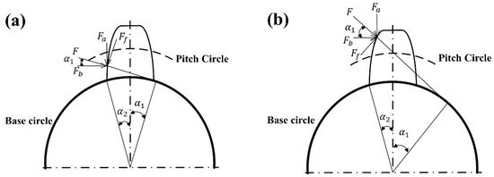
Figure 5.
Direction of Friction Force on the Drive Gear.
For the driven gear, the engagement phase extends from the tooth crest B to the node, while the disengagement phase spans from the node to the tooth root D. The direction of friction force is tangential to the tooth surface and points toward the node. Neither the driving nor driven gear experiences friction at the node.
As shown in Figure 5, during the meshing stage of the drive gear, the components of the tooth-surface contact force in the and directions, due to tooth-surface friction, are:
During the bite-out phase, the tooth-surface contact force component is:
In the equation, represents the tooth-surface friction force, calculated as , where is the coefficient of friction. The friction coefficient is dependent on sliding velocity and contact pressure, representing a parameter with complex computational characteristics [24]. To simplify the analysis, this study introduces only tangential stiffness for the qualitative assessment of friction effects, with the friction coefficient defined as a constant of appropriate magnitude.
Substituting Equations (19) and (20), which account for tooth-surface friction, into Equations (1)–(3), and performing the same simplifications as before, the bending stiffness, shear stiffness, and axial compression stiffness of the driving and driven gears can be expressed as:
Among the various types of teeth, the upper teeth are in the biting-in phase, while the lower teeth are in the biting-out phase.
Figure 6 shows the meshing stiffness curve with friction correction applied to a single tooth compared to the curve without friction. Analysis and comparison using Equations (21)–(23) and Figure 6 reveal that during the meshing of a single gear pair, tooth-surface friction causes changes in the values of the three potential energies during the meshing phase, thereby increasing the meshing stiffness during this phase. Conversely, during the disengagement phase, a sudden change in the direction of tooth-surface friction causes the changes in the three potential energies to be opposite to those during the meshing phase, resulting in a decrease in meshing stiffness. When this abrupt change occurs at the node, the friction direction at the node undergoes a sudden shift, causing the magnitude of the meshing stiffness to change abruptly. The meshing stiffness calculated without considering tooth-surface friction does not exhibit abrupt changes in the friction correction value, and thus does not show abrupt changes in meshing stiffness.
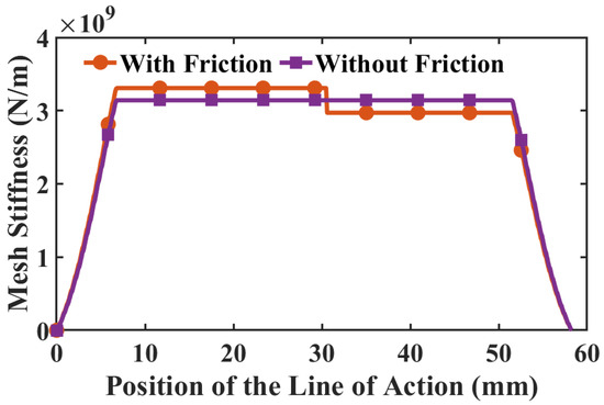
Figure 6.
Comparison of Single-Tooth Friction Engagement Stiffness (Under rated load).
Figure 7 shows the comprehensive variation curve of meshing stiffness under multi-tooth engagement conditions. Analysis reveals that regardless of whether tooth-surface friction is considered, the minimum value of the comprehensive meshing stiffness curve for helical gears remains identical. Since tooth-surface friction increases stiffness during the meshing initiation phase, the stiffness curve accounting for friction exhibits higher values than the friction-free curve during both the ascending and amplitude phases. During the disengagement phase, a sudden change in friction direction causes the meshing stiffness to decrease. Consequently, in the descending phase, the curve considering friction initially exceeds the curve without friction consideration. Subsequently, a sudden change occurs, causing the friction-considered curve to fall below the friction-excluded curve. Finally, as the curves approach their minimum values, they converge toward consistency.
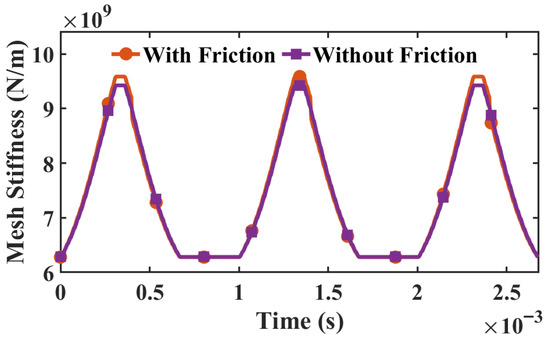
Figure 7.
Comparison of Multi-Tooth Friction Engagement Stiffness (Under rated load).
2.3. Analytical Method for Engagement Stiffness Considering Contact Deformation at Contact Points
The contact deformation is illustrated in Figure 8. During the meshing phase of a gear pair, the meshing line can be considered as composed of multiple contact points based on the slicing method. Under load, the tooth surfaces of each slice undergo elliptical contact patch deformation, which similarly affects the time-varying meshing stiffness of each slice.
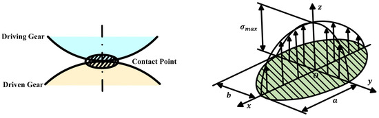
Figure 8.
Local elliptical deformation and stress distribution at the tooth-surface contact point.
Based on the slice potential energy method and under the premise that a nonlinear coupling relationship exists between tooth-surface load and local deformation, the local deformation at a contact point on any slice during gear meshing can be obtained by calculating Equation (24).
In Equation (24), denotes the normal force at contact point , is the thickness of a single slice, is the elastic modulus, is Poisson’s ratio, and represent the distances from the contact point to point , the intersection of the normal line and the tooth centerline, on the driving and driven gears, respectively, and is the half-width of contact along the tooth profile direction, expressed as . and are the curvature radii of the driving and driven gears at the contact point, respectively. According to the properties of involute gears, the curvature radius at a contact point equals the distance from that point to the tangent point on the base circle. Given the meshing angle at the contact point and the base circle radius, its curvature radius can be readily calculated. The schematic of the parameters is shown in Figure 3.
By combining the aforementioned calculation formulas, it can be seen that the normal flexibility of the tooth surface can be obtained by superimposing the Hertzian contact flexibility, bending flexibility, shear flexibility, axial compression flexibility of the driving and driven gears, and the equivalent flexibility of the gear body section. The calculation formula is:
In the formula, denotes the driving wheel, and denotes the driven wheel.
The macroscopic linear deformation at contact point is:
The elastic deformation coordination condition for contact point is:
In the equation, represents the actual convergence amount generated at contact point between the two gears, i.e., the transmission error; is the original error at contact point . The schematic diagram of and is shown in Figure 9. In the right-hand inequality, when , it takes a value greater than zero, indicating contact at point , where . When , it takes a value equal to zero, indicating no contact at point , where .
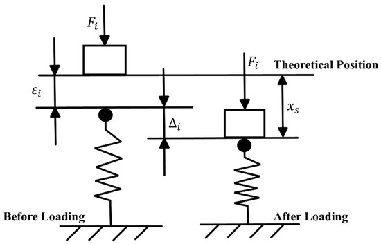
Figure 9.
Schematic Diagram of Deformation Before and After Loading at Tooth-Surface Contact Point .
The matrix form of Equation (27) is:
At the same time, load-balancing conditions must be satisfied during contact:
By solving Equations (28) and (29) iteratively, the contact point load vector and transmission error can be obtained. Summing the stiffness at each contact point yields the meshing stiffness of the gear pair, accounting for local tooth-surface deformation: .
The above steps can be summarized as a two-level iterative solution procedure, as follows:
- (1)
- Set and assign an initial transmission error .
- (2)
- Sequentially evaluate the deformation at each contact point ; if it is less than 0, set it to 0.
- (3)
- Use the golden-section method to iteratively solve the nonlinear Equation (28), obtaining the load distribution vector , and calculate the total load .
- (4)
- Check whether holds (where is the allowable tolerance). If not, update , with being the average macroscopic deformation coefficient of all contact points, set , and return to step (2); if it holds, terminate the iteration and output , .
- (5)
- The mesh stiffness of the gear pair is obtained by summing the stiffness at each contact point: .
Figure 10 shows the meshing stiffness curves for a single tooth, comparing those with and without local deformation iteration. Comparative analysis reveals that while the peak meshing stiffness decreases when local deformation iteration is incorporated, the overall trend remains largely unchanged.
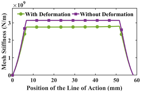
Figure 10.
Iterative Comparison of Local Deformation in a Single Tooth (Under rated load).
Figure 11 shows the variation curve of meshing stiffness under multi-tooth engagement conditions. Comparative analysis reveals that the conclusion remains consistent with single-tooth engagement: the effect of local deformation is limited to reducing overall meshing stiffness. The overall meshing stiffness decreases by approximately 10%, with no significant impact on the fluctuation trend of the meshing stiffness curve.
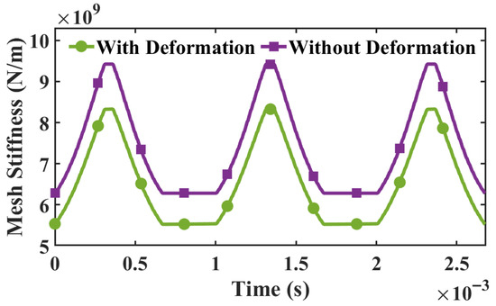
Figure 11.
Comparison of Iterative Local Deformation for Multi-Tooth Components (Under rated load).
2.4. Analytical Method for Engagement Stiffness Considering Tooth-Surface Friction and Local Contact Deformation
Figure 12 presents the variation curve of meshing stiffness that comprehensively considers tooth-surface friction and contact point deformation. Comparative analysis reveals that the analytical method incorporating both tooth-surface friction and local contact deformation yields the same conclusion as the previous analysis: the meshing stiffness curve obtained from the optimized analytical method is approximately 10% lower overall than that from the slice potential energy method. During meshing, abrupt changes in the direction of frictional forces cause numerical discontinuities in the meshing stiffness curve.
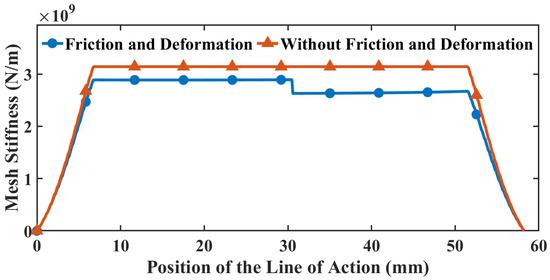
Figure 12.
Comparison of Single-Tooth Engagement Stiffness Curves Using the Optimized Analytical Method (Under rated load).
Figure 13 presents the variation curve of meshing stiffness under multi-tooth engagement, accounting for tooth-surface friction and contact point deformation. Comparative analysis reveals that the overall meshing stiffness curve exhibits a noticeable numerical decrease due to the influence of contact deformation. The range of meshing stiffness fluctuations derived from the slice potential energy method spans from to , whereas the optimized analytical method accounting for tooth-surface friction and contact point deformation yields a fluctuation range of to . Additionally, due to the abrupt change in friction direction at nodes caused by tooth-surface friction, the meshing stiffness curve calculated by the proposed optimized analytical method exhibits a distinct abrupt change during its decline phase. The original slicing potential energy method does not exhibit this abrupt change phenomenon. Additionally, this paper compares the meshing stiffness curves obtained from the optimization analysis method with those from the finite element method. It can be observed that both the amplitude and fluctuation trends of the meshing stiffness are identical, demonstrating the accuracy and reliability of the proposed method.
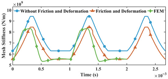
Figure 13.
Comparison of Multi-Tooth Engagement Stiffness Curves Using the Optimized Analytical Method (Under rated load).
Based on the above analysis, it can be seen that the proposed optimization analytical method, building upon the highly reliable slice potential energy approach, incorporates additional tooth-surface factors, thereby making the theoretical calculation method more closely aligned with practical conditions.
3. Application of Optimized Time-Varying Meshing Stiffness Models in Sound Field Calculations for Gear Reducers
To validate the reliability of the proposed optimized meshing stiffness calculation method, this study applied it to a rapid acoustic radiation prediction model for locomotive traction drive systems based on the contact line method [32]. By replacing the stiffness algorithm in the original model and conducting acoustic simulations, the predicted sound pressure level results before and after optimization were compared and analyzed, thereby providing evidence for the effectiveness of the proposed method. The acoustic simulations in this study are conducted based on COMSOL [33].
3.1. Contact Line Method
Reference [32] employs the contact line method to calculate time-varying mesh stiffness and subsequently establishes a rapid acoustic radiation modeling approach for locomotive traction transmission systems. During gear pair meshing, the tooth contact zone generally appears as a band-shaped region whose length is substantially greater than its width. Hence, the contact line method simplifies these band-shaped regions into contact lines distributed along the tooth width. Relying on the assumption that mesh stiffness is proportional to the contact line length, the time-varying mesh stiffness is derived from the variation in contact line length and the average mesh stiffness.
Figure 14 illustrates the variation in the contact line length during the meshing of a single tooth pair. When , the maximum contact line length is ; when , the maximum contact line length is . Since the contact line length undergoes three distinct phases, increasing, constant, and decreasing, during a single tooth meshing cycle, it can be expressed as the product of the maximum contact line length and a piecewise function , as given below:
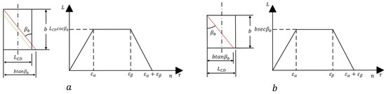
Figure 14.
Variation in Contact Length on Single-Pair Teeth (a) ; (b) [32].
The meshing process of a gear pair involves multiple-tooth engagement; thus, after obtaining the expression for the single-tooth contact line length, the total contact line length at any instant can be derived by superposition, as follows:
where , with being the ceiling function, is the total contact ratio, , and denote the angular velocity and base circle radius of the driving gear, respectively, and is the base pitch of the helical gear.
The theoretical single-tooth stiffness can be calculated using an empirical formula based on ISO standards, as follows:
In the formula, and represent the equivalent tooth numbers of the driving and driven gears, calculated as . and denote the normal displacement coefficients of the driving and driven gears.
Considering actual operating conditions, the theoretical stiffness must be modified to obtain the maximum single-tooth stiffness :
In the formula, represents the gear pair modification coefficient, reflecting the stiffness enhancement effect of profile and directional modifications; denotes the blank structure coefficient, accounting for the stiffness reduction due to blank flexibility; and signifies the tooth width coefficient, considering the reduction in effective stiffness caused by uneven load distribution resulting from large tooth width.
Considering the influence of overlap, the formula for calculating the average stiffness per tooth pair within one meshing cycle is:
Convert the average single-tooth stiffness into contact stiffness per unit length , establishing a mapping relationship between stiffness and geometric length:
In the formula, represents the maximum contact line length, and denotes the tooth width.
Based on the core assumptions of the contact method, the instantaneous meshing stiffness of a gear pair is proportional to the instantaneous total contact line length , expressed as:
3.2. Comparison of the Optimized Slice Potential Method and the Contact Line Method
To compare whether the optimized slice potential method and the contact line method yield significantly different results in solving meshing stiffness, both methods must be applied to calculate the gear pair used in the locomotive traction transmission system. Detailed gear parameters are provided in Table 2.
As shown in Figure 15, the engagement stiffness curve calculated using the optimized potential energy method exhibits no difference in its overall trend compared to the engagement stiffness fluctuation curve obtained from the contact line method. The values are only slightly lower than those from the contact line method, with a numerical difference of approximately 5%. Since the contact line method relies on empirical formulas, which generally yield values higher than the actual engagement stiffness, it can be concluded that the optimized method achieves higher accuracy compared to the contact line method.
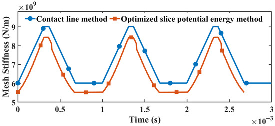
Figure 15.
Comparison of the optimized slice potential energy method and the contact line method.
3.3. Comparison of Acoustic Simulation Results Between the Optimized Slicing Potential Method and the Contact Line Method
In the rapid modeling method for sound radiation in locomotive traction transmission systems, the core computational data consists of three components: gear meshing noise, bearing force excitation on the housing generated by gear meshing, and motor operating noise. These three datasets are input into an acoustic simulation model to calculate the average sound pressure level in the external sound field [32].
Based on the analysis of locomotive traction transmission systems, it is evident that operating conditions significantly influence bearing force excitation. As one of the most critical nonlinear factors in gear systems, variations in meshing stiffness substantially affect bearing force excitation. Therefore, while keeping other parameters in the model constant, such as bearing stiffness and damping, operating conditions, and load, a comparison between the acoustic calculation results obtained before and after replacing the meshing stiffness calculation method in the theoretical model and the actual acoustic measurement data from locomotive traction transmission systems can determine whether the optimized meshing stiffness calculation method offers higher accuracy and reliability.
Figure 16 shows the near-field sound pressure level distribution of the traction drive system under operating condition 5. Similar to the results obtained using the original meshing stiffness calculation method, the figure reveals that the highest sound pressure levels occur within the enclosure. Within the air domain, the peak sound pressure level distribution is located between the motor and the transmission. Applying the same calculation procedure to the remaining five operating conditions demonstrates that variations in operating conditions do not alter the near-field distribution of sound pressure levels. This indicates that changes in meshing stiffness do not influence the near-field distribution of sound pressure levels.
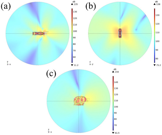
Figure 16.
Near-field sound pressure level distribution under operating condition 5 ((a) XY plane; (b) YZ plane; (c) XZ plane).
Figure 17 presents the average sound pressure level measured at 4 m from the traction transmission system under six operating conditions, calculated using two theoretical models with different mesh stiffness methods. The six operating conditions are 20 km/h, 30 km/h, 40 km/h, 50 km/h, 60 km/h, and 114 km/h, respectively. To validate the reliability of the method, acoustic test data from actual vehicle measurements were compared with theoretical acoustic calculation results. Analysis shows that as train speed increases, the total sound pressure level obtained by both stiffness calculation methods exhibits a trend of first increasing and then decreasing: the sound pressure level from the contact line method rises from 81.3 dB to 88 dB before falling to 77.3 dB, while that from the optimized slice potential energy method increases from 80 dB to 88.6 dB and then declines to 77.3 dB. Observation reveals that the experimentally measured sound pressure level rises from 80.5 dB to 88.3 dB before decreasing to 85.56 dB, matching both the magnitude and trend of the two theoretical methods. Notably, the maximum discrepancy between the contact line method and the measured data occurs under operating condition 3, where the theoretical value is 84.2 dB and the measured value is 88.3 dB, with a maximum error within 5%. In contrast, the maximum deviation for the optimized slice potential energy method appears under operating condition 2, with a theoretical value of 82.76 dB and a measured value of 80.97 dB, resulting in a maximum error of only 2.2%. Beyond this, the results of the optimized slice potential energy method align more consistently with the actual trend, and its sound pressure level peak occurs under operating condition 3, consistent with the real-vehicle test data. Combined with the comparative results in Section 3.2, the overall decrease in mesh stiffness will lead to a reduction in natural frequency, implying that the locomotive operating speed corresponding to the resonance peak will also decrease. This inference aligns with the observation in Figure 17 that the sound pressure level peak shifts from condition 5 (contact line method) to condition 3 (slice potential energy method), supporting that the optimized slice potential energy method proposed in this study achieves higher accuracy in mesh stiffness calculation than the contact line method. In summary, the optimized slice potential method exhibits higher accuracy than the contact line method in modeling locomotive traction transmission systems.
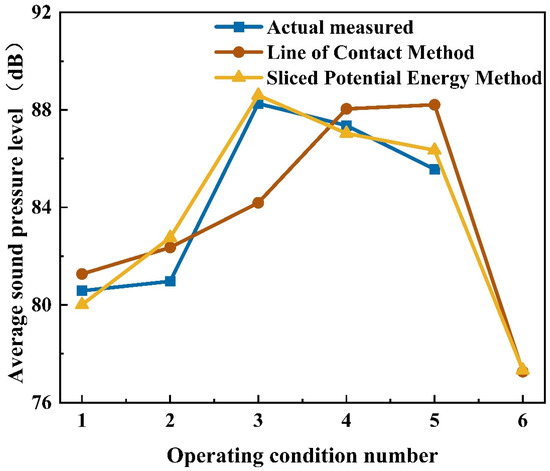
Figure 17.
Average Sound Pressure Level at 4 m from the Traction Drive System under Different Operating Conditions [32].
4. Conclusions
This paper proposes an optimized analytical method for meshing stiffness. Based on the slice potential energy approach, this method accounts for tooth-surface friction and local deformation, enabling the calculated results to follow the variation trend of meshing stiffness during gear engagement more closely than those from the conventional method. As shown in the comparative analysis of Section 2.4, the calculated results exhibit high consistency with finite element simulation outcomes, with a maximum amplitude error not exceeding 1%, thereby validating the data reliability. When applied to a rapid modeling method for acoustic radiation in locomotive traction transmission systems, the maximum error in sound pressure level data decreased from approximately 5% using the contact method to 2.2%. Furthermore, the peak distribution aligns with experimental data, confirming the accuracy and reliability of this optimized approach in practical applications. This optimization facilitates more dependable analysis results when using rapid modeling methods to investigate the intrinsic relationship between design parameters and dynamic responses.
Calculation results indicate that the optimization method differs from the traditional slice potential method primarily in the overall reduction of meshing stiffness values and the presence of abrupt changes in the curve. As analyzed in Section 2.2, abrupt changes in the direction of tooth-surface friction cause corresponding abrupt changes in the meshing stiffness curve, resulting in higher stiffness during the meshing phase and lower stiffness during the disengagement phase. As analyzed in Section 2.3, considering local deformation of the tooth surfaces does not significantly alter the trend of the meshing stiffness curve, but the values decrease by approximately 10%.
Author Contributions
Z.Y.: conceptualization, methodology, software, investigation, formal analysis, writing—original draft. K.Y.: data curation, writing—original draft, visualization, investigation. J.Z.: conceptualization, resources, supervision, writing—review and editing. All authors have read and agreed to the published version of the manuscript.
Funding
This research received no external funding.
Institutional Review Board Statement
Not applicable.
Informed Consent Statement
Not applicable.
Data Availability Statement
The original contributions presented in this study are included in the article. Further inquiries can be directed to the corresponding author.
Conflicts of Interest
The authors do not have any conflicts of interest with other entities or researchers.
Nomenclature
| Bending potential energy | |
| Shear potential energy | |
| Axial compressive potential energy | |
| Hertzian contact potential energy | |
| Bending stiffness | |
| Shear stiffness | |
| Axial compressive stiffness | |
| Hertzian contact stiffness | |
| Resultant force acting on the meshing teeth at the contact point | |
| Radial force | |
| Tangential force | |
| Shear modulus | |
| Young’s modulus | |
| Area moment of inertia | |
| Cross-sectional area | |
| Distance from the tooth root | |
| Tooth width | |
| Poisson’s ratio | |
| Distance from gear contact point to tooth root | |
| Half of the tooth thickness at the contact point | |
| Total equivalent meshing stiffness | |
| Meshing angle at the start of engagement | |
| Meshing angle at the end of engagement | |
| Amount of deformation in the wheel body | |
| Wheel body deformation stiffness | |
| Distance from the intersection point of the contact point normal line and the tooth centerline to the tooth root | |
| Tooth root thickness | |
| Calculation function for wheel body deformation | |
| Half of the tooth thickness angle | |
| Tooth root radius | |
| Gear inner radius | |
| Ratio of tooth root radius to gear inner radius | |
| Coefficient of friction | |
| Contact half-width in the profile direction | |
| Curvature radius of the driving and driven gears at the contact point | |
| Slice width | |
| Distance from the contact point along the normal direction to the gear centerline | |
| Hertzian contact flexibility | |
| Bending flexibility | |
| Shear flexibility | |
| Axial compression flexibility | |
| Total flexibility | |
| Macroscopic linear deformation | |
| Actual convergence amount | |
| Original error | |
| Local contact deformation | |
| Total load | |
| Time-varying contact line length for a single tooth pair | |
| Periodic piecewise linear function | |
| Total contact line length | |
| Theoretical single-tooth stiffness | |
| Maximum single-tooth stiffness | |
| Average stiffness | |
| Contact stiffness per unit length | |
| Instantaneous meshing stiffness |
References
- Li, Z.; Li, H.; Ren, C.; Deng, Y.; Cao, J.; Xiong, J.; Zhou, B.; Bai, H.; Zhang, H.; Wang, S.; et al. Low-Velocity Impact Resistance of All Composite Cylindrical Shell Panels with a Foam Filled Honeycomb Core: Theoretical and Experimental Investigation. Int. J. Impact Eng. 2023, 182, 104765. [Google Scholar] [CrossRef]
- Chang, L.; Liu, G.; Wu, L. A Robust Model for Determining the Mesh Stiffness of Cylindrical Gears. Mech. Mach. Theory 2015, 87, 93–114. [Google Scholar] [CrossRef]
- Kiekbusch, T.; Sappok, D.; Sauer, B.; Howard, I. Calculation of the Combined Torsional Mesh Stiffness of Spur Gears with Two- and Three-Dimensional Parametrical FE Models. J. Mech. Eng. 2011, 57, 810–818. [Google Scholar] [CrossRef]
- Zhan, J.; Fard, M.; Jazar, R. A CAD-FEM-QSA Integration Technique for Determining the Time-Varying Meshing Stiffness of Gear Pairs. Measurement 2017, 100, 139–149. [Google Scholar] [CrossRef]
- Tian, X.; Zuo, M.J.; Fyfe, K.R. Analysis of the Vibration Response of a Gearbox with Gear Tooth Faults. In Proceedings of the ASME International Mechanical Engineering Congress and Exposition, Anaheim, CA, USA, 13–19 November 2004; pp. 785–793. [Google Scholar]
- Sainsot, P.; Velex, P.; Duverger, O. Contribution of Gear Body to Tooth Deflections—A New Bidimensional Analytical Formula. J. Mech. Des. 2004, 126, 748–752. [Google Scholar] [CrossRef]
- Han, L.; Xu, L.; Qi, H. Influences of Friction and Mesh Misalignment on Time-Varying Mesh Stiffness of Helical Gears. J. Mech. Sci. Technol. 2017, 31, 3121–3130. [Google Scholar] [CrossRef]
- Huangfu, Y.; Chen, K.; Ma, H.; Li, X.; Han, H.; Zhao, Z. Meshing and Dynamic Characteristics Analysis of Spalled Gear Systems: A Theoretical and Experimental Study. Mech. Syst. Signal Process. 2020, 139, 106640. [Google Scholar] [CrossRef]
- Chen, K.; Huangfu, Y.; Ma, H.; Xu, Z.; Li, X.; Wen, B. Calculation of Mesh Stiffness of Spur Gears Considering Complex Foundation Types and Crack Propagation Paths. Mech. Syst. Signal Process. 2019, 130, 273–292. [Google Scholar] [CrossRef]
- Cai, Y. Simulation on the Rotational Vibration of Helical Gears in Consideration of the Tooth Separation Phenomenon (A New Stiffness Function of Helical Involute Tooth Pair). J. Mech. Des. 1995, 117, 460–469. [Google Scholar] [CrossRef]
- Umezawa, K.; Suzuki, T.; Sato, T. Vibration of Power Transmission Helical Gears: Approximate Equation of Tooth Stiffness. Bull. JSME 1986, 29, 1605–1611. [Google Scholar] [CrossRef]
- Velex, P. On the Modelling of Spur and Helical Gear Dynamic Behaviour. In Mechanical Engineering; Gokcek, M., Ed.; InTech: Rijeka, Croatia, 2012. [Google Scholar]
- Qin, Y.; Li, Q.; Wang, S.; Cao, P. Dynamics Modeling of Faulty Planetary Gearboxes by Time-Varying Mesh Stiffness Excitation of Spherical Overlapping Pittings. Mech. Syst. Signal Process. 2024, 210, 111162. [Google Scholar] [CrossRef]
- Hedlund, J.; Lehtovaara, A. A Parameterized Numerical Model for the Evaluation of Gear Mesh Stiffness Variation of a Helical Gear Pair. Proc. Inst. Mech. Eng. C 2008, 222, 1321–1327. [Google Scholar] [CrossRef]
- Dell’Accio, F.; Guessab, A.; Nudo, F. New quadratic and cubic polynomial enrichments of the Crouzeix–Raviart finite element. Comput. Math. Appl. 2024, 170, 204–212. [Google Scholar] [CrossRef]
- Chen, Z.; Zhai, W.; Shao, Y.; Wang, K.; Sun, G. Analytical Model for Mesh Stiffness Calculation of Spur Gear Pair with Non-Uniformly Distributed Tooth Root Crack. Eng. Fail. Anal. 2016, 66, 502–514. [Google Scholar] [CrossRef]
- Yu, W.; Shao, Y.; Mechefske, C.K. The Effects of Spur Gear Tooth Spatial Crack Propagation on Gear Mesh Stiffness. Eng. Fail. Anal. 2015, 54, 103–119. [Google Scholar] [CrossRef]
- Yang, H.; Shi, W.; Chen, Z.; Guo, N. An Improved Analytical Method for Mesh Stiffness Calculation of Helical Gear Pair Considering Time-Varying Backlash. Mech. Syst. Signal Process. 2022, 170, 108882. [Google Scholar] [CrossRef]
- Wan, Z.; Cao, H.; Zi, Y.; He, W.; He, Z. An improved time-varying mesh stiffness algorithm and dynamic modeling of gear-rotor system with tooth root crack. Eng. Fail. Anal. 2014, 42, 157–177. [Google Scholar] [CrossRef]
- Wu, X.; Luo, Y.; Li, Q.; Shi, J. A New Analytical Model for Evaluating the Time-Varying Mesh Stiffness of Helical Gears in Healthy and Spalling Cases. Eng. Fail. Anal. 2022, 131, 105842. [Google Scholar] [CrossRef]
- Li, F.; Li, H.; Zhai, J.; Yuan, M.; Sun, B.; Dong, Z. Improved analytical model of gear mesh stiffness considering free end effect and contact gap variation. Appl. Math. Model. 2025, 151, 116460. [Google Scholar] [CrossRef]
- Zhao, Z.; Han, H.; Wang, P.; Ma, H.; Zhang, S.; Yang, Y. An improved model for meshing characteristics analysis of spur gears considering fractal surface contact and friction. Mech. Mach. Theory 2021, 158, 104219. [Google Scholar] [CrossRef]
- Li, Z.; Chen, H.; Chen, J.; Zhu, R. Analytical impact of the sliding friction on mesh stiffness of spur gear drives based on Ishikawa model. Vibroengineering Procedia 2014, 4, 29–33. [Google Scholar]
- Marjanovic, N.; Ivkovic, B.; Blagojevic, M.; Stojanovic, B. Experimental determination of friction coefficient at gear drives. J. Balk. Tribol. Assoc. 2010, 16, 517–526. [Google Scholar]
- Dai, H.; Long, X.; Chen, F.; Xun, C. An Improved Analytical Model for Gear Mesh Stiffness Calculation. Mech. Mach. Theory 2021, 159, 104262. [Google Scholar] [CrossRef]
- Flek, J.; Dub, M.; Kolář, J.; Lopot, F.; Petr, K. Determination of Mesh Stiffness of Gear—Analytical Approach vs. FEM Analysis. Appl. Sci. 2021, 11, 4960. [Google Scholar] [CrossRef]
- Yu, W.; Mechefske, C.K. A New Model for the Single Mesh Stiffness Calculation of Helical Gears Using the Slicing Principle. Iran. J. Sci. Technol. Trans. Mech. Eng. 2019, 43, 503–515. [Google Scholar] [CrossRef]
- Hou, S.; Wei, J.; Zhang, A.; Zhang, C.; Yan, J.; Wang, C. A Novel Comprehensive Method for Modeling and Analysis of Mesh Stiffness of Helical Gear. Appl. Sci. 2020, 10, 6695. [Google Scholar] [CrossRef]
- Tang, X.; Zou, L.; Yang, W.; Huang, Y.; Wang, H. Novel Mathematical Modelling Methods of Comprehensive Mesh Stiffness for Spur and Helical Gears. Appl. Math. Model. 2018, 64, 524–540. [Google Scholar] [CrossRef]
- MATLAB, version R2023b; Software for Numerical Computing; The MathWorks, Inc.: Natick, MA, USA, 2023.
- Ma, H.; Song, R.; Pang, X.; Wen, B. Time-varying mesh stiffness calculation of cracked spur gears. Eng. Fail. Anal. 2014, 44, 179–194. [Google Scholar] [CrossRef]
- Li, C.; Liu, X.; Yu, K.; Yang, Z.; Zhang, J.; Li, P. A Rapid Modeling Method for Sound Radiation of China’s Locomotive Traction Drive Systems in Railways. Appl. Sci. 2025, 15, 10597. [Google Scholar] [CrossRef]
- COMSOL Multiphysics, version 6.2; Software for Multiphysics Simulation; COMSOL AB: Stockholm, Sweden, 2023.


Disclaimer/Publisher’s Note: The statements, opinions and data contained in all publications are solely those of the individual author(s) and contributor(s) and not of MDPI and/or the editor(s). MDPI and/or the editor(s) disclaim responsibility for any injury to people or property resulting from any ideas, methods, instructions or products referred to in the content. |
© 2026 by the authors. Licensee MDPI, Basel, Switzerland. This article is an open access article distributed under the terms and conditions of the Creative Commons Attribution (CC BY) license.