Research on TID Controller Design for Fractional-Order Time-Delay Systems

Abstract

Fractional-order time-delay systems boast better dynamic performance than integer-order ones in optimally controlling industrial design objects. However, in lack of commendable methodologies, designing proper controllers for these systems confronts a plurality of challenges. This study puts forth an innovative design approach that merges frequency-domain analysis with time-domain optimization concepts, so that fractional-order Tilt-Integral-Derivative (TID) controllers can be acquired. To pursue a stable control system loop, the tilted and integral gains of fractional-order TID controllers are identified as per frequency-domain specifications, including gain crossover frequency and phase margin. In light of these specifications (e.g., the integral of time-weighted absolute error (ITAE)), the differential gain and fractional-order operator $\lambda$ of the controller are determined, which accomplishes a desirable dynamic performance in the time domain. This article expounds on the procedure of how to develop the proposed fractional-order TID controller and furnishes illustrative examples for the research steps. As manifested by the simulation results, the proposed controller dramatically upgrades the control performance of the system in contrast to conventional PID, FOPI, and FOPID controllers. Moreover, it outperforms PID and fuzzy PID in terms of responding to the demand variations in step signals.

1. Introduction

Fractional-order operators provide enhanced modeling flexibility and more accurate dynamic representation for industrial time-delay systems compared to integer-order approaches [1,2]. Such systems exhibit overdamped or critically damped behavior, which complicates controller design in industrial process control [3]. The introduction of fractional-order elements in the Laplace domain boosts the degrees of freedom in system representation, enabling more precise modeling under varied damping conditions and supporting the design of higher-performance controllers [4].

To fully exploit these advantages, fractional-order controllers—such as the TID controller—have been developed. The fractional-order TID controller extends conventional PID control by incorporating fractional-order operators, thereby offering additional tuning parameters and improved regulation capability [5,6,7]. Current tuning methods for fractional-order controllers mainly fall into two categories: frequency-domain techniques, which ensure stability through specifications like gain crossover frequency and phase-margin [8], and time-domain optimization approaches, which target optimal transient response [9,10]. However, recent advances reveal a persistent gap between these two philosophies. Methods that strictly enforce frequency-domain specifications, such as fixed phase margin or gain crossover frequency [11], ensure robust stability but often lack explicit guarantees on transient performance. Conversely, strategies focused on optimizing time-domain indices like ITAE can achieve excellent dynamic response but may compromise robustness margins. While integrated approaches utilizing flat-phase constraints or D-partition methods have been attempted [12,13], they typically address stability, robustness, and performance objectives in a sequential or decoupled manner. This leaves the unified co-design of these critical attributes—particularly for fractional-order TID control of time-delay systems—inadequately explored.

To address this gap, we propose a unified design method for fractional-order TID controllers that simultaneously satisfies both frequency- and time-domain specifications. The main contributions are as follows:

(1) A systematic design procedure for fractional-order TID controllers is developed, integrating both frequency- and time-domain requirements to enhance the dynamic performance of fractional-order time-delay systems.

(2) The D-partition method is employed to delineate the parameter space that ensures closed-loop stability.

(3) A complete design workflow is presented and validated through simulation case studies, demonstrating that the proposed controller outperforms conventional PID, FOPI, and FOPID controllers in both set-point tracking and disturbance rejection. Additionally, the controller’s response to step-signal variations across different time intervals is evaluated and compared with PID and fuzzy PID strategies.

The structure of this article is as follows: Section 2 introduces the fractional-order time-delay system model and the transfer function of the fractional-order TID controller. Section 3 hinges on the D-partition method to derive control system parameters and dissect the parameter space for system stability. Section 4 delineates the design process for the optimal fractional-order TID controller based on fractional-order time-delay systems, and the simulation findings in Section 5 imply the more favorable control performance of the designed controller than PID, FOPI, and FOPID controllers. Compared with the PID and fuzzy PID control strategies, the control strategy of fractional-order TID has a better and faster response effect to the demand-based variations in step signals.

2. System Controller and Design Process

2.1. Mathematical Model of Fractional-Order Time-Delay (FOTD) Systems

In industrial control processes, there are commonly time delays in the mathematical transfer functions of real controlled systems, and mathematical models of time-delay systems represent real-world controlled systems in a more accurate manner [14]. Previous efforts have affirmed that, regarding industrial control, the time-delay system models involving fractional-order operators better procure the dynamic characteristics of system control processes than traditional integer-order ones. So far, these fractional-order operator-based time-delay systems have been broadly applied to mathematical modeling and simulation processes in industrial engineering [4].

The mathematical transfer function model of this fractional-order time-delay (FOTD) system can be given as below:

$$G_p\left(s\right)={\displaystyle \frac{K}{T{s}^{\mu }+1}}{e}^{-Ls}$$

(1)

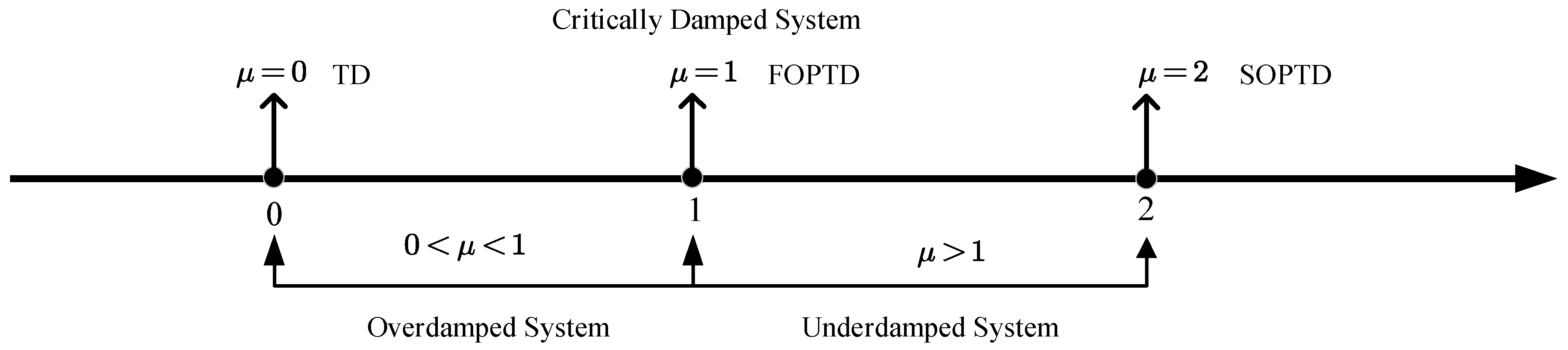
where $\mu$ signifies the fractional-order operator, the value of $\mu$ ranges within $0<\mu <2$; $T$ denotes the time scalar (where $T$ is a fractional-order time constant possessing the dimension of $s^{\mu }$); $K$ symbolizes the system gain; and $L$ means the time-delay parameter. When $\mu =0$, the foregoing controlled system evolves into a simple time-delay (TD) one; for $\mu =1$, the controlled system is a first-order plus time-delay (FOPTD) system [15]; in the case of $\mu =2$, the controlled system is a second-order plus time-delay (SOPTD) system [12]; and when $\mu >2$, the system turns into a higher-order time-delay one, which deteriorates the complexity of control system computation and stability analysis in industrial control engineering [16]. When fractional-order values are taken for $\mu$, the fractional-order time-delay systems with various damping conditions are garnered, as illustrated in Figure 1.

2.2. Mathematical Model of Fractional-Order TID Controller

For the fractional-order TID controller proposed in this study, the mathematical model of the transfer function is expressed as:

$$G_t\left(s\right)={\displaystyle \frac{K_t}{s^{\lambda }}}+{\displaystyle \frac{K_i}{s}}+K_{d}s$$

(2)

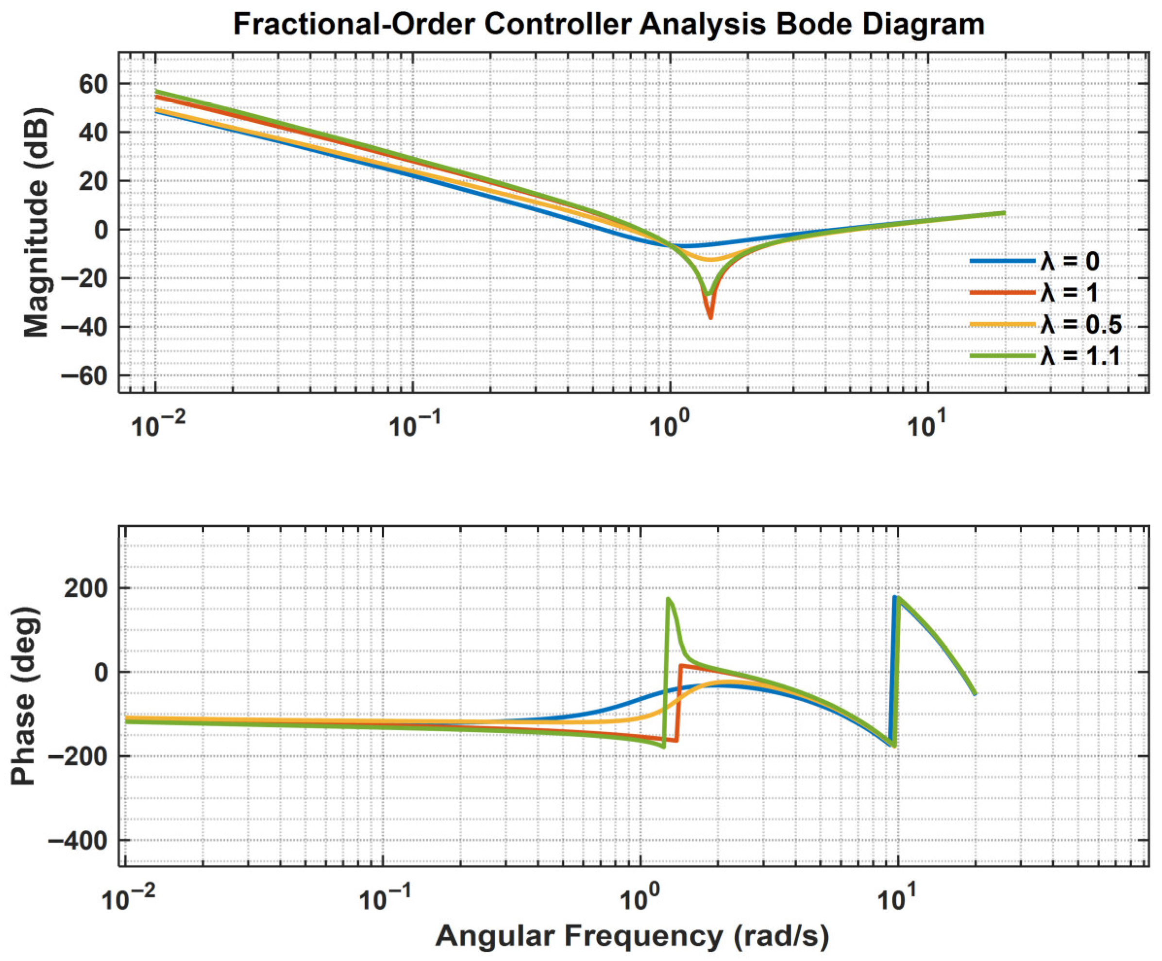
where $K_t$, $K_i$, $K_d$, stand for the tilt gain, integral gain, and differential gain, respectively. $\lambda$ designates the fractional-order operator of the controller to be designed, whose value range is $\lambda \in \left(0,2\right)$. When $\lambda =0$, the foregoing controller model represents a traditional PID controller; In the case of $\lambda$ as an integer-order, the controller model implies an integer-order TID controller; when $\lambda =1$, it acts as a traditional first-order TID controller; When $0<\lambda <2$, the controller model represents the fractional-order TID controller to be designed. Given $K_t=1$, $K_i=1$, $K_d=1$, when $\lambda$ varies, the Bode plots illustrating these controller types are depicted in Figure 2.

.

2.3. Design Procedure of TID Controller Based on Fractional-Order Time-Delay Systems

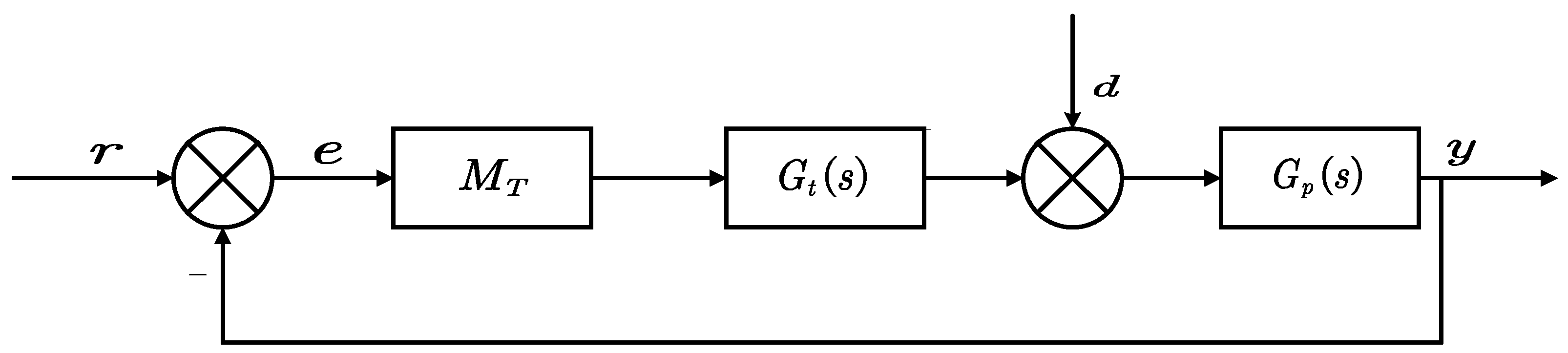
Figure 3 portrays the closed-loop fractional-order TID control system based on the fractional-order time-delay system. Where $r$, $d$, $y$ denotes the actual input signal, actual disturbance signal, and actual output signal, respectively, and $e$ signifies the actual error signal. In addition, $M_T$ means a gain-phase margin tester involved for plotting controller parameter boundaries and establishing the system’s phase margin $\varphi$ and gain margin $A$, where the expression for $M_T$ is $M_T\left(A,\varphi \right)=A{e}^{-j\varphi }$. $G_t\left(s\right)$ stands for the controlled fractional-order time-delay system, and $G_p\left(s\right)$ symbolizes the fractional-order TID controller to be designed.

The procedure for computing the transfer function of closed-loop system in Figure 3 is exhibited as below:

$${\displaystyle \frac{Y\left(s\right)}{R\left(s\right)}}={\displaystyle \frac{M_T{G}_p\left(s\right)G_t\left(s\right)}{1+M_T{G}_p\left(s\right)G_t\left(s\right)}}$$

(3)

where $R\left(s\right)$, $U\left(s\right)$, $Y\left(s\right)$ serve as the Laplace transforms of $r$, $u$, $y$, respectively. Substituting each expression into Equation (3) yields:

$$\varphi \left(s\right)={\displaystyle \frac{Y\left(s\right)}{R\left(s\right)}}={\displaystyle \frac{AK{e}^{-j\varphi -Ls}\left(K_t{s}^{1-\lambda }+K_i+K_d\cdot s^2\right)}{s\cdot \left(T{s}^{\mu }+1\right)+AK{e}^{-j\varphi -Ls}\left(K_t{s}^{1-\lambda }+K_i+K_d\cdot s^2\right)}}$$

(4)

From Equation (4), the characteristic polynomial of the closed-loop system is garnered as:

$$D\left(s\right)=s\cdot \left(T{s}^{\mu }+1\right)+AK{e}^{-j\varphi -Ls}\left(K_t{s}^{1-\lambda }+K_i+K_d\cdot s^2\right)$$

(5)

The relationship between the distribution positions of these characteristic roots and the stability of the closed-loop control system can be determined based on all characteristic roots of the closed-loop system’s characteristic polynomial $D\left(s\right)=0$ and the Laplace final value theorem [17]. According to prior research, if all characteristic roots of the closed-loop system’s characteristic polynomial $D\left(s\right)=0$ lie within the left half-plane of the s-domain, it can be deduced that the closed-loop control system is stable [18]. In this study, when $A=1$, $\varphi =0$, the closed-loop control system is stable within a bounded-input bounded-output region, provided all roots of $D\left(s\right)=0$ are situated in the left half-plane of the s-domain.

The four unknown parameters of the closed-loop system’s characteristic polynomial $D\left(s\right)$ are continuous numerical values, so the root locus of the polynomial $D\left(s\right)=0$ is also continuous within the parameter space where the stability of the closed-loop system is retained. Characteristic roots of the closed-loop system cross the imaginary axis of the s-domain in three ways: $s=0, s=j\omega , s=\infty$. By means of D-partition [19], unknown parameters ensuring system stability can be identified, so as to construct the stable parameter space bounded by Real Root Boundary (RRB, $s=0$), Complex Root Boundary (CRB, $s=j\omega$) and Infinite Root Boundary (IRB, $s=\infty$).

The three characteristic root crossings through the imaginary axis in the s-domain can be defined as follows:

• RRB: $D\left(s=0\right)=0$, substituting into Equation (5) and solving yields the unknown parameter $K_i$

  $$K_i=0$$

  (6)
• CRB: $D\left(s=j\omega \right)=0$, substituting into Equation (5) and solving gains the following equations:

  $$\left\{\begin{array}{l}{K}_t\cdot {\omega }^{1-\lambda }\cdot \left(C_2\cdot C_3+S_2\cdot S_3\right)+C_3\cdot K_i-C_3\cdot K_d\cdot {\omega }^2-T\cdot {\omega }^{1+\mu }\cdot S_1=0\hfill \\ K_t\cdot {\omega }^{1-\lambda }\cdot \left(S_2\cdot C_3-C_2\cdot S_3\right)-S_3\cdot K_i+S_3\cdot K_d\cdot {\omega }^2+T\cdot {\omega }^{1+\mu }\cdot C_1+\omega =0\hfill \end{array}\right.$$

  (7)

Part of the polynomial equations in Equation (7) are defined as:

$$\begin{gathered} C_1=\cos \left({\displaystyle \frac{\pi }{2}}\mu \right)\hspace{0.33em}\hspace{0.33em};\hspace{0.33em}\hspace{0.33em}{S}_1=\sin \left({\displaystyle \frac{\pi }{2}}\mu \right) \\ {C}_2=\cos \left({\displaystyle \frac{\pi }{2}}\cdot \left(1-\lambda \right)\right)\hspace{0.33em}\hspace{0.33em};\hspace{0.33em}\hspace{0.33em}{S}_2=\sin \left({\displaystyle \frac{\pi }{2}}\cdot \left(1-\lambda \right)\right) \\ {C}_3=K\cdot \cos \left(\varphi +\omega L\right)\hspace{0.33em}\hspace{0.33em};\hspace{0.33em}\hspace{0.33em}{S}_3=K\sin \left(\varphi +\omega L\right) \end{gathered}$$

The values of the unknown parameters $K_t$, $K_i$ acquired are given as below:

$$\left\{\begin{array}{l}{K}_t={\displaystyle \frac{T\cdot {\omega }^{1+\mu }\left(S_1\cdot S_3-C_1\cdot C_3\right)-\omega \cdot C_3}{S_2\cdot w^{1-\lambda }\cdot {\left(K\right)}^2}}\hfill \\ K_i={\displaystyle \frac{T\cdot {\omega }^{1+\mu }\cdot S_1\cdot \left(C_3\cdot S_2-S_3\cdot C_2\right)+\left(T\cdot {\omega }^{1+\mu }\cdot C_1+\omega \right)\cdot \left(C_2\cdot C_3+S_2\cdot S_3\right)}{S_2\cdot {\left(K\right)}^2}}+K_d\cdot {\omega }^2\hfill \end{array}\right.$$

(8)

In the resulting Equation (8), $C_3^2+S_3^2={\left(K\right)}^2$.

• IRB: $D\left(s=\infty \right)=0$, substituting into Equation (5) and solving produces the following equations:

  $$\left\{\begin{array}{l}(j\omega )\cdot \left(T\cdot {(j\omega )}^{\mu }+1\right)=-K{e}^{-j(\varphi +\omega L)}\cdot \left(K_t\cdot {(j\omega )}^{1-\lambda }+K_i+K_d\cdot {(j\omega )}^2\right)\hfill \\ (-j\omega )\cdot \left(T\cdot {(-j\omega )}^{\mu }+1\right)=-K{e}^{-j(\varphi -\omega L)}\cdot \left(K_t\cdot {(-j\omega )}^{1-\lambda }+K_i+K_d\cdot {(-j\omega )}^2\right)\hfill \end{array}\right.$$

  (9)

When $\omega \to \infty$, $\left|e^{j\varphi }\right|=1$, the following can be generated by multiplying the upper and lower equations in Equation (9) and retaining merely the highest-order polynomial terms on both sides $\omega$:

$${\omega }^2\cdot T^2\cdot {\left({\omega }^{\mu }\right)}^2={\left(K{e}^{-j\varphi }\right)}^2\cdot K_d^2\cdot {\omega }^4$$

(10)

Solving Equation (10) results in the value of the unknown parameter $K_d$:

$$K_d=\pm {\displaystyle \frac{T\cdot {\omega }^{\mu }}{K}}$$

(11)

Given $A=1$, $\varphi =0°$, the values of relevant unknown parameters are confirmed through the foregoing calculation process. The parameter space region where the closed-loop control system is stable can thus be drawn, which is divided into stable and unstable areas. Verification of a randomly selected test point within the region ascertains the stable area [20], and all parameters of the fractional-order TID controller simultaneously falling into a stable area convey that the closed-loop control system is basically stable.

3. Fractional-Order TID Controller Design Method Based on Combined Time-Domain and Frequency-Domain Analysis

In pursuit of more robust dynamic performance of fractional-order time-delay systems, frequency-domain analysis is merged with time-domain design methods, in order to develop fractional-order TID controllers for fractional-order time-delay systems.

3.1. Frequency-Domain Specifications of Fractional-Order TID Controller

In frequency-domain analysis, the predefined objectives are represented by the gain crossover frequency ${\omega }_c$, the phase margin ${\varphi }_m$, and the flat-phase constraint condition.

The gain crossover frequency and phase margin are expressed as blow:

• Gain crossover frequency

$${\left|C\left(j{\omega }_c\right)P\left(j{\omega }_c\right)\right|}_{dB}=0$$

(12)

• Phase margin

$$arg\left[C\left(j{\omega }_c\right)P\left(j{\omega }_c\right)\right]=-\pi +{\varphi }_m$$

(13)

The gain-phase margin tester $M_T$ (set as $A=1$ here) can be leveraged to determine the gain and phase margin parameters of a given control system [21].

A flat-phase bode plot at ${\omega }_c$ implies that the control system preserves constant overshoot as the closed-loop gain varies [22]. The flat-phase constraint condition can be represented as:

• Flat-phase constraint

$${\displaystyle \frac{d{\varphi }_m}{d{\omega }_c}}=0$$

(14)

3.2. Time-Domain Specifications of Fractional-Order TID Controller

There are four unknown parameters for the fractional-order TID controller to be designed. To sustain the consistency between the number of unknown parameters and design criteria, this work introduces time-domain specifications, such as the integral time-weighted absolute error (ITAE) [23].

• ITAE

  $$J_{ITAE}={\displaystyle {\int }_0^{\infty }t\left|e\left(t\right)\right|}dt$$

  (15)

  where $e\left(t\right)$ denotes the difference signal between the actual input signal and the actual output signal. The system performance is evaluated using the $J_{ITAE}$ criterion (where $J$ denotes the performance index).

3.3. Parameter Determination Procedure for Fractional-Order TID Controller

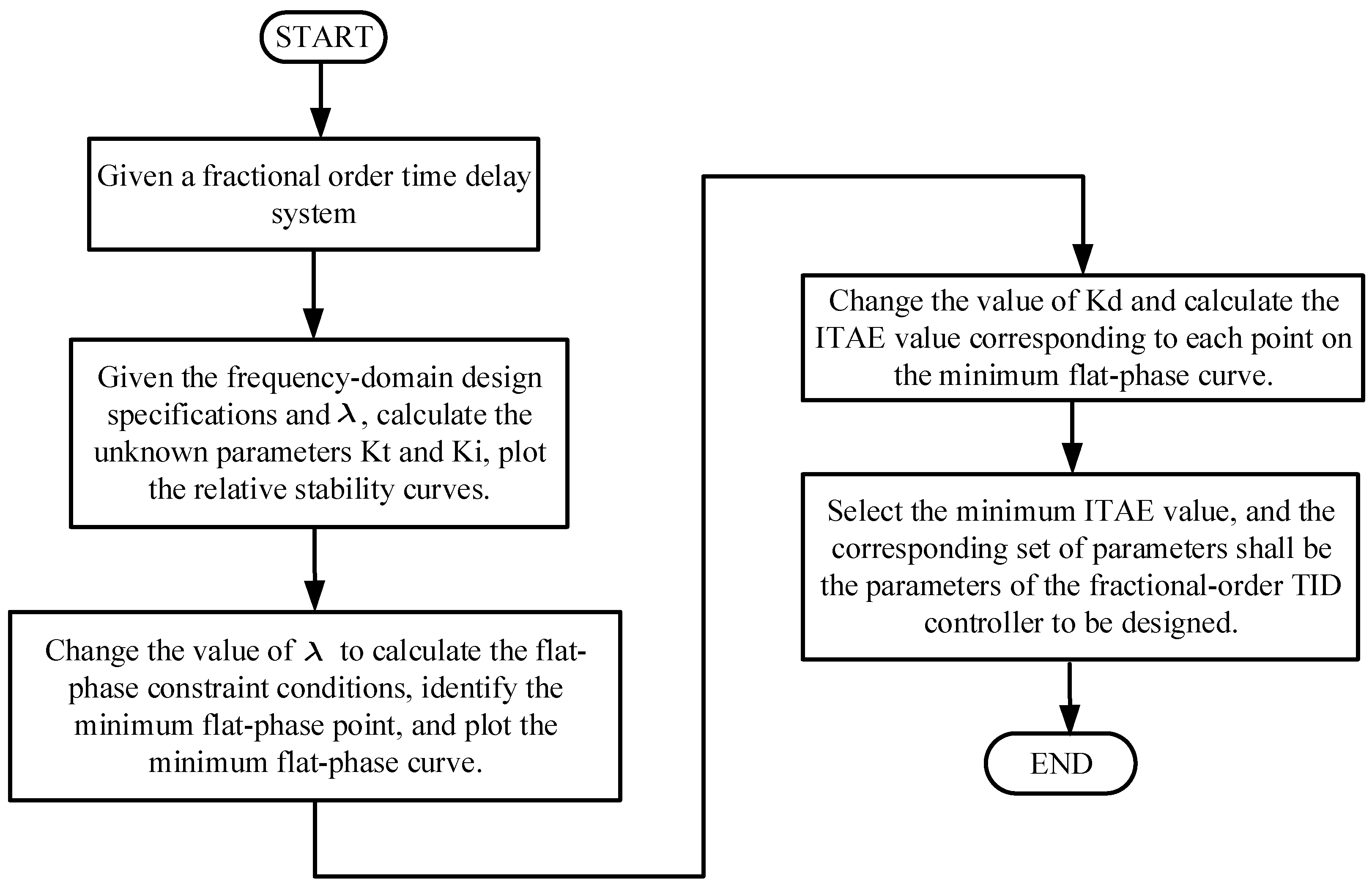
(1) Given a fractional-order time-delay system, fixed value $\lambda$, and gain crossover frequency ${\omega }_0$, Equations (6) and (8) are employed to derive the parameter values that abide by the given stability margin $\varphi ={\varphi }_m$ with $A=1$ for system stability, so that the parameter space is attained for system stability to be plotted.

(2) Alongside a fixed $K_d$ satisfying $\varphi ={\varphi }_m$ with $A=1$, the $K_t-K_i$ relative stability curves for varying values of $\omega$ are plotted within the parameter space when $\omega \to {\omega }_{\max }$. Here, ${\omega }_{\max }$ designates the maximum frequency within the parameter space, and all points on the relative stability curve are in alignment with the specified phase margin ${\varphi }_m$ requirement.

(3) To guarantee a flat-phase bode plot at ${\omega }_0$, the above parameter values are substituted into Equations (7) and (14), so as to compute the flat-phase constraint condition, portray the flat-phase curve, and confirm the minimum flat-phase point.

Solving Equations (7) and (14) yields:

$${\displaystyle \frac{d\varphi }{d\omega }}=-L+{\displaystyle \frac{\left({N_1}^2+{N_2}^2\right)\left(M_1{M_2}^{\prime }-M_2{M_1}^{\prime }\right)+\left({M_1}^2+{M_2}^2\right)\left(N_1{N_2}^{\prime }-N_2{N_1}^{\prime }\right)}{{\left(M_1{N}_1-M_2{N}_2\right)}^2+{\left(M_1{N}_2+M_2{N}_1\right)}^2}}=0$$

(16)

Within the resulting Equation (16), the partial algebraic expressions are defined as below:

$$\begin{array}{c}{M}_1^{\prime }=(1-\lambda )\cdot K_t\cdot {\omega }^{-\lambda }\cdot C_2-2K_d\cdot \omega \hspace{0.33em}\hspace{0.33em}\hspace{0.33em}{M}_2^{\prime }=(1-\lambda )\cdot K_t\cdot {\omega }^{-\lambda }\cdot S_2\\ N_1^{\prime }=(1+\mu )\cdot T\cdot {\omega }^{\mu }\cdot S_1\hspace{0.33em}\hspace{0.33em}\hspace{0.33em}{N}_2^{\prime }=(1+\mu )\cdot T\cdot {\omega }^{\mu }\cdot C_1+1\end{array}$$

(4) Then, the study traverses all values within the $\lambda \in \left(0,2\right)$ interval, computes the set of all flat-phase points that meet both gain crossover frequency and phase margin requirements and sustain flatness at ${\omega }_0$, and depicts the minimum flat-phase curve comprising the minimum flat-phase points garnered by varying each $\lambda$ value.

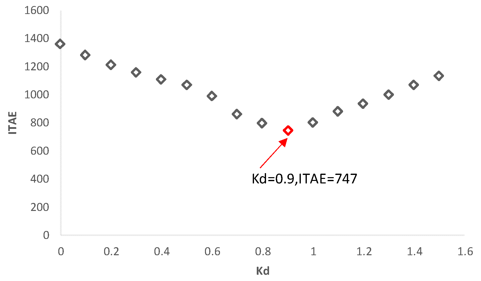
(5) Steps (2)–(4) are repeated after changing the value of $K_d$, and step-response simulations are performed in numerical simulation software for each set of unknown parameters $\left(K_t,K_i,\lambda ,K_d\right)$ corresponding to points on the minimum flat-phase curve. ITAE value is calculated for each set of unknown parameters, while plotting ITAE as a function of varying $K_d$, and its minimum is identified.

(6) The unique set of unknown parameters for ITAE’s minimum designates the parameters of the fractional-order TID controller that simultaneously comply with the frequency-domain requirements and time-domain specifications.

Figure 4 visualizes the foregoing procedure for determining fractional-order TID controller parameters.

4. Fractional-Order TID Controller Design Example

The design of fractional-order TID controller is delineated by the following example.

Step 1: Based on a fractional-order time-delay system [24], given a gain crossover frequency of ${\omega }_c=$ 0.7 rad/s, and a phase margin of ${\varphi }_m=60°$, the transfer function of the fractional-order time-delay system can be expressed as:

$$G_p\left(s\right)={\displaystyle \frac{5}{10s^{0.5}+1}}{e}^{-0.4s}$$

(17)

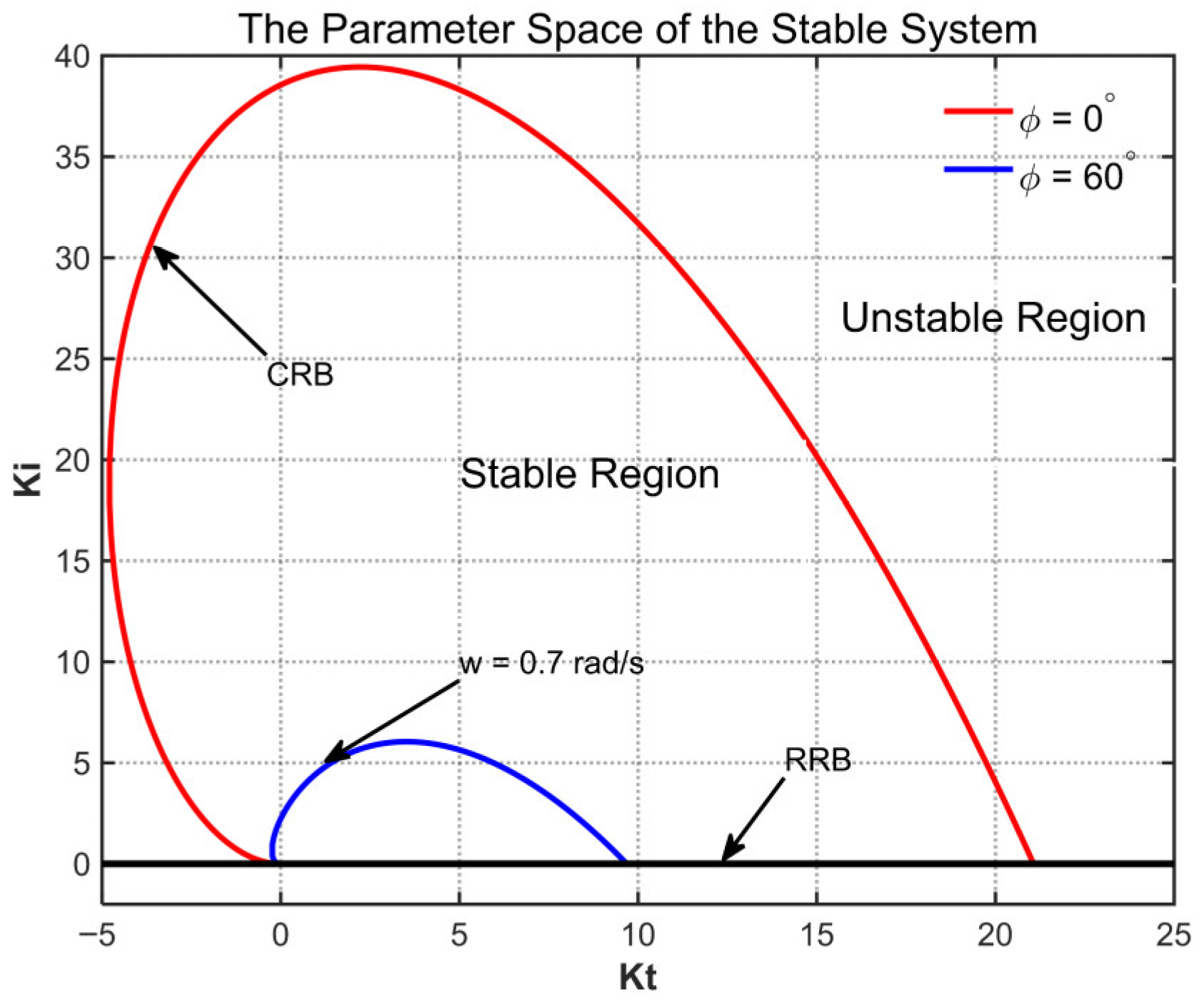
Step 2: With $K_d=1$ and $\lambda =0.5$ fixed, $K_t$ and $K_i$ values are calculated via Equations (6) and (8). The RRB and CRB curves are portrayed for the parameter space corresponding to system stability. As unveiled in Figure 5 [Source code in Supplementary Code: Parameter stable region], the blue curve stands for the CRB curve at $\varphi$ = 60°, and the black curve for the RRB curve. After the random point tests within the parameter space enclosed by the CRB and RRB curves [25], the stable and unstable parameter regions can be determined for the system.

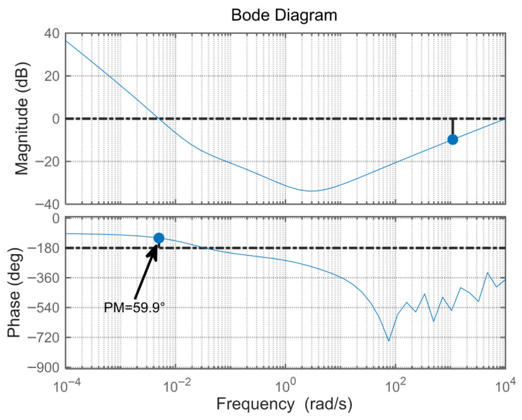
Figure 6 [Source code in Supplementary Code: Bode plot] illustrates the open-loop bode plot of the control system with $A=1$, ${\varphi }_m=60°$, apart from a phase margin (PM) of $59.9°$. A phase margin error of $0.1°$ lies within the permissible range. Consequently, it is corroborated that the fractional-order TID controller accomplishes the required system control performance.

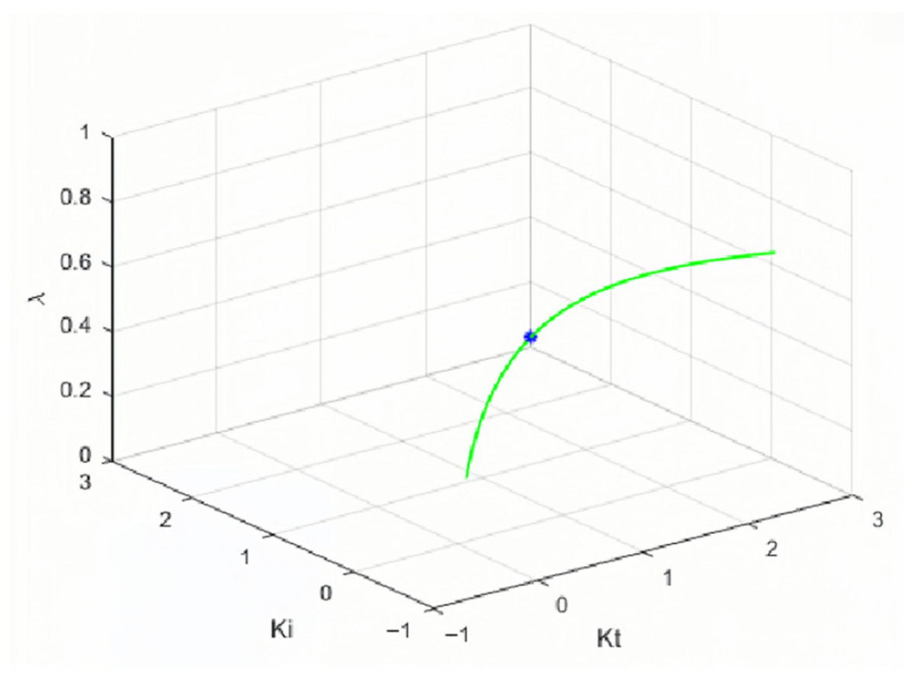
Step 3: With the fixed values of ${\omega }_c=$ 0.7 rad/s and $\lambda =0.5$, the flat-phase constraint is computed using Equation (16), and the flat-phase curve is plotted as shown by the green curve in Figure 7 [Source code in Supplementary Code: Flat phase constraint]. The minimum flat-phase point is marked in blue.

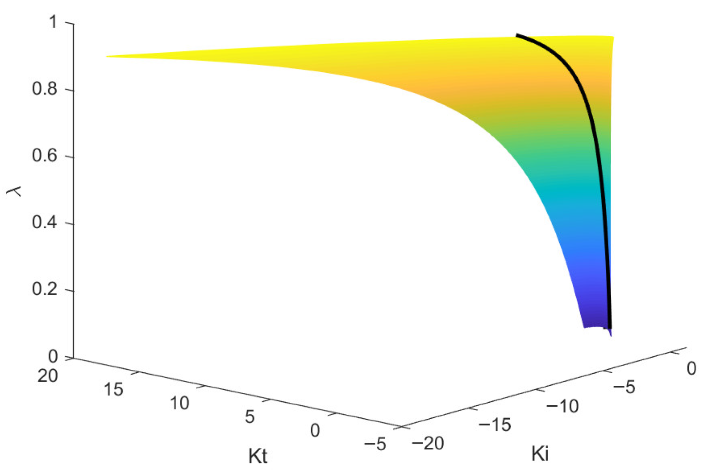
Step 4: Given $K_d=1$, the study traverses all values of $\lambda$ within the interval (0,2), repeats Step 3, and plots the surface conforming to the flat-phase constraint condition, according to Figure 8 [Source code in Supplementary Code: ITAE calculate]. The minimum flat-phase points for each value of $\lambda$ generate the minimum flat-phase curve, which is depicted in black in Figure 8. All points on this curve fulfill the conditions of ${\omega }_c=$ 0.7 rad/s, ${\varphi }_m=60°$, and the minimum flat-phase constraint.

Step 5: $K_d\in \left(-2\cdot {0.7}^{0.5},\hspace{0.33em}+2\cdot {0.7}^{0.5}\right)$ is derived through Equation (11). By varying $K_d$, step-response simulations are undertaken for each parameter set ($K_t,K_i,\lambda$) that designates each point on the black curve in Figure 8. The study computes ITAE values for these parameter sets as $K_d$ changes, plots the results of ITAE versus $K_d$ in view of Figure 9 [Source code in Supplementary Code: ITAE calculate], and highlights the minimal ITAE in red. As for the parameter values ($K_t,K_i,\lambda ,K_d$) corresponding to the red ITAE point, they denote the fractional-order TID controller parameters that comply with both frequency-domain requirements and time-domain optimization specifications.

The fractional-order TID controller obtained thereby is in agreement with both frequency-domain requirements and time-domain optimization criteria, so that the accuracy is boosted for controller parameter design.

5. Simulation Results and Analysis

For the purpose of affirming the benefits of the proposed method, as per identical frequency-domain specifications for all controllers, this study leans on numerical simulation examples to compare the fractional-order TID controller designed using the proposed method with those PID, FOPI, and FOPID controllers derived otherwise. The performance indices originating from distinguishable control systems are analyzed, while the ability of the proposed strategy to withstand varying levels of external disturbance is assessed. Meanwhile, this study analyzes the rapidity and accuracy of the response to step signal demand of the fractional-order TID control strategy proposed here, in comparison with those of the PID and fuzzy PID control strategies.

5.1. Simulation Results of Fractional-Order TID Control System

• Sample 1

Under the frequency-domain conditions [26] of ${\omega }_c=$ 0.7 rad/s, ${\varphi }_m=60°$, the expression of the fractional-order TID controller (acquired from calculations in Section 4) is given as below:

$$G_{TID-proposed}\left(s\right)={\displaystyle \frac{0.6162}{s^{0.9}}}+{\displaystyle \frac{0.3188}{s}}+0.69s$$

(18)

Under the same conditions, the PID [27], FOPI [28], and FOPID [6] controllers are, respectively, expressed as follows:

$$G_{PID}\left(s\right)=2.738+{\displaystyle \frac{3.849}{s}}+2s$$

(19)

$$G_{FOPI}\left(s\right)=0.2173+{\displaystyle \frac{0.0378}{s^{1.34}}}$$

(20)

$$G_{FOPID}\left(s\right)=0.6428+{\displaystyle \frac{0.1201}{s^{1.89}}}+0.07s$$

(21)

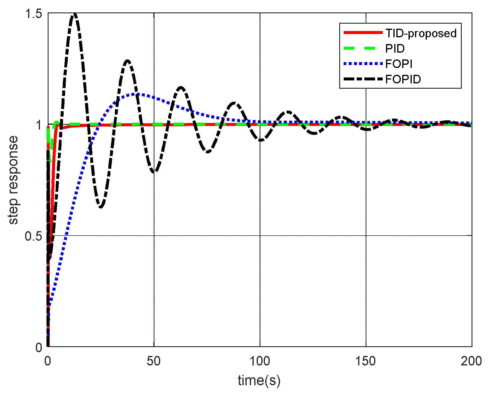
As visualized in Figure 10, the step-response results for the four control systems—TID, PID, FOPI, and FOPID—are encapsulated in

Table 1. Time-domain index results of four controllers.

Controller	Parameter				Results
	${\mathit{K}}_{\mathit{t}}$	${\mathit{K}}_{\mathit{i}}$	${\mathit{K}}_{\mathit{d}}$	$\mathit{\lambda }$	Overshoot (%)	Rise Time (s)	Settling Time (s)	Steady-State Error
PID	2.738	3.849	2	0	0.92873	0.24	2.61	0.000279
FOPI	0.2173	0.0378	0	1.34	13.094	19.57	83.32	0.000324
FOPID	0.6428	0.1201	0.07	1.89	49.714	5.52	152.83	0.000801
TID-Proposed	0.6162	0.3188	0.69	0.91	0.1597	0.08	3.82	0.000265

. The time-domain performance indices of the four control systems are summarized.

Figure 10 reveals that, among the four control systems, the overshoot is the smallest for the designed fractional-order TID controller which exhibits a faster rising process and attains stability in a shorter settling time. In the initial stage (0–30 s), the proposed TID controller exhibits the fastest rise time and almost no overshoot. This is due to the introduction of the fractional-order tilt term $K_t\cdot s^{-\lambda }$. Furthermore, the time-domain performance indices in Table 1 reflect that the designed controller accomplishes the smallest overshoot (0.1597%) and the shortest rise time (0.08 s) among the four controllers, and it reaps the best performance in light of the steady-state errors of the control system performance indices, despite the nuances in settling time among the four control systems. By employing the D-partition method to delineate a stability-guaranteed parameter space and then co-optimizing within it for both phase-margin and ITAE, the design attains a near flat-phase condition that reduces sensitivity to gain variations. This enables the selection of more aggressive yet stable parameters, resulting in the fast and oscillation-free convergence observed in the step response.

• Sample 2

Under the frequency-domain conditions [29] of ${\omega }_c=$ 0.03 rad/s, ${\varphi }_m=60°$, the expression of the fractional-order TID controller (acquired from calculations in Section 4) is given as below:

$$G_p\left(s\right)={\displaystyle \frac{0.3658}{79.2635s^{0.648}+1}}{e}^{-24.7360s}$$

(22)

The expression of the fractional-order TID controller derived by the design method proposed in this study is as follows:

$$G_{TID-proposed}\left(s\right)={\displaystyle \frac{4.1633}{s^{0.15}}}+{\displaystyle \frac{0.2211}{s}}+15.27s$$

(23)

Under the same conditions, the PID [30], FOPI [31], and FOPID [5] controllers are, respectively, expressed as follows:

$$G_{PID}\left(s\right)=10.5119+{\displaystyle \frac{0.21248}{s}}+130.0112s$$

(24)

$$G_{FOPI}\left(s\right)=9.9799+{\displaystyle \frac{0.0071}{s^{1.75}}}$$

(25)

$$G_{FOPID}\left(s\right)=14.002+{\displaystyle \frac{0.0094}{s^{1.89}}}-0.9s$$

(26)

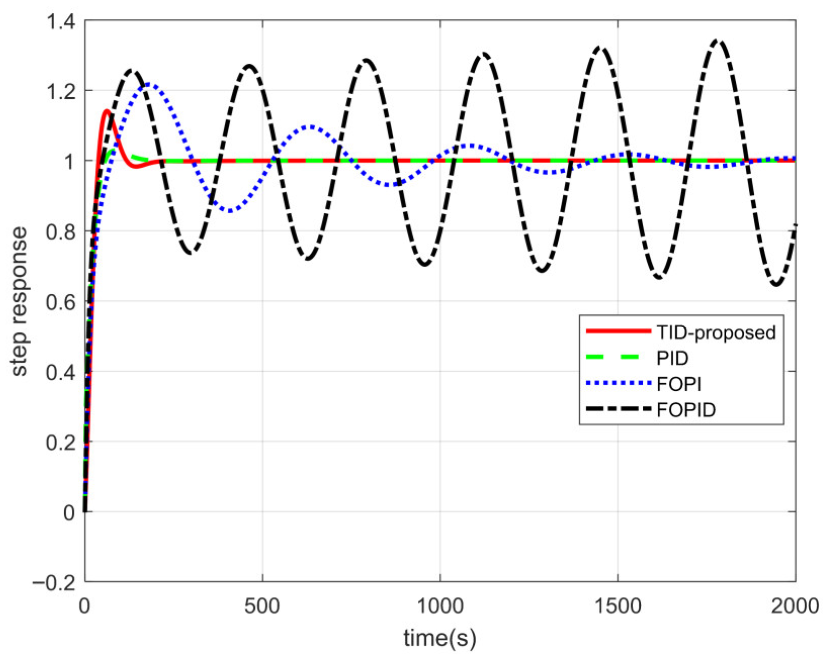
As visualized in Figure 11, the step-response results for the four control systems—TID, PID, FOPI, and FOPID—are encapsulated in

Table 2. Four control system time-domain index results for fractional-order time-delay systems.

Controller	Parameter (${\mathit{\omega }}_{\mathit{c}}$ = 0.03 rad/s, ${\mathit{\varphi }}_{\mathit{m}}$ = 60°)				Results
	${\mathit{K}}_{\mathit{t}}$	${\mathit{K}}_{\mathit{i}}$	${\mathit{K}}_{\mathit{d}}$	$\mathit{\lambda }$	Overshoot (%)	Rise Time (s)	Settling Time (s)	Steady-State Error
PID	10.5119	0.21248	130.0112	0	2.6696	31.53	137.65	0.0009586
FOPI	9.9799	0.0071	0	1.75	20.915	47.14	1808.6	0.0061439
FOPID	14.002	0.0094	−0.9	1.89	63.77	42.56	1997.1	0.018041
TID- Proposed	4.1633	0.2211	15.27	0.15	13.736	17.2	114.86	0.0000355

. The time-domain performance indices of the four control systems are summarized.

Figure 11 reveals that, for the fractional-order time-delay system, the fractional-order TID controller designed in this study exhibits relatively superior overshoot performance among the four control systems, while also featuring a better rising process and a faster settling time. The fractional-order tilt term $K_t\cdot s^{-\lambda }$ provides a phase contribution of $\lambda \cdot 90°$, which is continuously variable with $\lambda$. Unlike the fixed −90° shift from a standard integrator, it allows for independent adjustment of the system’s phase curve in the mid-frequency range. This fine-tuning enables a high gain crossover frequency and a fast rise time while maintaining sufficient phase margin. The results in Table 2 show that the proposed fractional-order TID controller achieves the minimum rise time (17.2 s) and settling time (114.86 s) among the four control systems. Based on the steady-state error, a key performance index of the control system, the designed fractional-order TID controller delivers the optimal performance among the four. However, in terms of overshoot, the performance of the four control systems varies slightly. Merely adding a fractional-order operator is insufficient, as their oscillatory responses indicate. Using the D-partition method, a stability-guaranteed parameter space is first established. Within this constrained region, a unified optimization is performed to simultaneously satisfy phase-margin and a time-domain index ITAE. This co-design process finds the globally optimal combination of the integer gains ($K_t,K_i,K_d$) and the fractional order $\lambda$, which traditional sequential tuning cannot achieve.

5.2. Demand-Based Variations Response of Step Signals

In the actual design process of the control system, due to the differences in the setting of expected targets, it may be necessary to set the external environment with demand-based variations for the control system in different time periods, so as to achieve the demand-based control effects corresponding to different time periods [32,33].

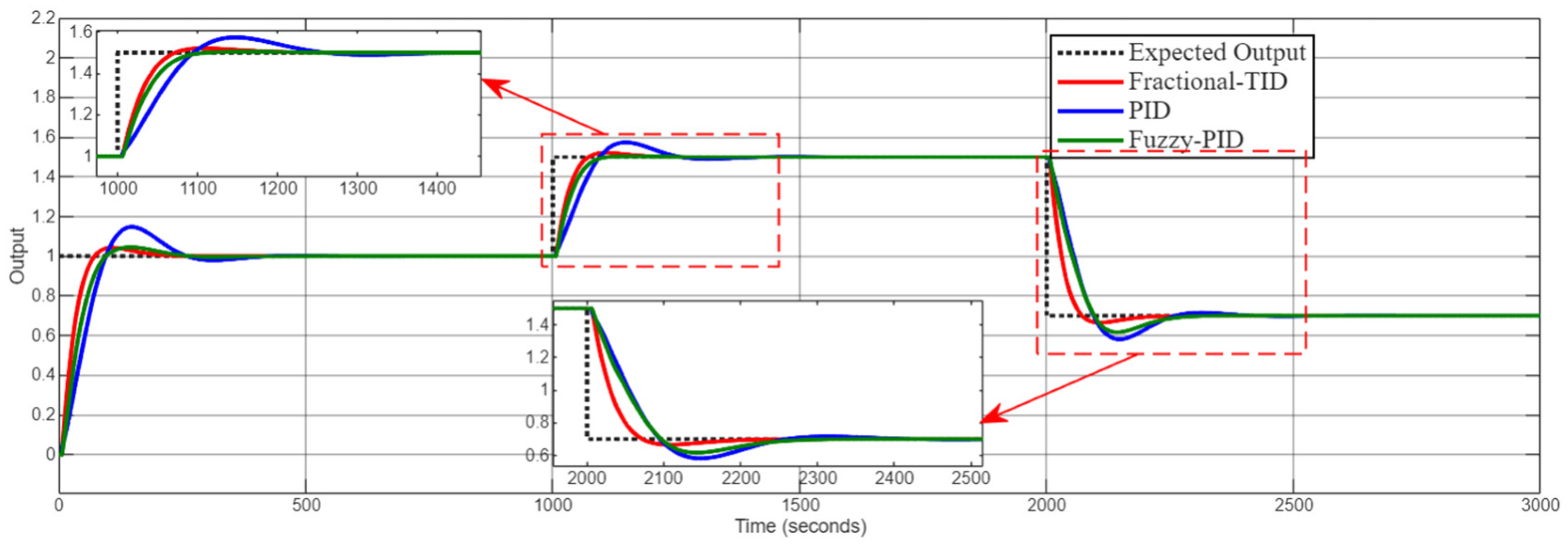
The design process is as follows: the input signal of the control system is a step signal, and the expected output of the system is one. The design process of the demand-based variation in the step signal is defined as: at 1000 s after the control system stabilizes, the input signal value of the control system is abruptly increased to 1.5 to observe the stability of the system; then, at 2000 s, the input signal of the system is abruptly decreased to 0.7 due to external requirements. The total simulation time of the control system is 1000 s. The output responses of the three control systems after the demand-based mutation of the step signal are observed and analyzed, as shown in Figure 12 below.

Table 3. Time-domain results of the three control systems after demand-based variation in step signals.

Controller Type	${\mathit{t}}_{\mathit{r}}$ (s)	${\mathit{t}}_{\mathit{s}}$ (s)	Overshoot (%)	${\mathit{t}}_{\mathit{r}}$ (s)	${\mathit{t}}_{\mathit{s}}$ (s)	Overshoot (s)
	Input Signal Increase to 1.5 at 1000 s			Input Signal Decrease to 0.7 at 1000 s
PID	97	374	35	101	357	33
fuzzy PID	124	203	2	92	303	27
Fractional-TID	63	192	11	62	271	13

summarizes the time-domain results of the three control systems after demand-based variation in step signals. The fractional-order operator $s^{-\lambda }$ provides a phase contribution of $\lambda \cdot 90°$, which is continuously variable with $\lambda$; thus, it can compensate for the phase lag of the time-delay system. At 1000 s after the control systems reached a steady state, the input signal abruptly increases to 1.5. At this moment, the fractional-order TID control strategy achieved a rise time of 63 s and a settling time of 192 s, exhibiting the best performance among the three control strategies. These results translate to the rapid, almost overshoot-free transitions observed in the red curve at each set-point step. However, the fractional-order TID control strategy yielded an overshoot of 11%, which was higher than the 2% overshoot of the fuzzy PID control strategy but lower than the 35% overshoot of the PID control strategy. After the control systems returned to a steady state, the input signal abruptly decreases to 0.7 at 2000 s. The fractional-order TID control strategy attained a rise time of 62 s, a settling time of 271 s, and an overshoot of 13%, again delivering the best performance among the three control strategies. A comprehensive analysis shows that even when subject to external demand variation in step signals, the fractional-order TID control strategy still maintains favorable adaptability and can better track the setpoint of the control system. This combination provides the necessary design freedom to break the classic speed-versus-overshoot trade-off, resulting in the fast, smooth, and robust responses evident in the control system.

6. Summary

6.1. Conclusions

For fractional-order time-delay systems, this study proposes a design method for the fractional-order TID controller parameters. As a result, a fractional-order TID controller is derived, which boasts commendable time-domain performance, and abides by frequency-domain specifications. The D-synthesis method is leveraged during the design of the fractional-order TID controller, allowing the fractional-order TID control system to meet frequency-domain indices including gain crossover frequency and phase margin. A unique set of fractional-order TID controller parameters is determined by means of identifying the minimum flat-phase point and conducting step-response simulation calculations for the parameter set to acquire the time-domain indicator ITAE. Through the simulations of fractional-order time-delay systems, the controller designed via the proposed method displays significant overshoot improvements over PID, FOPI, and FOPID controllers gained otherwise. Dramatic augmentations are also noticed in rise time and settling time, alongside smaller steady-state error. Compared with the PID and fuzzy PID control strategies, the fractional-order TID control strategy adopted in this study achieves a shorter settling time and a smaller overshoot in the response process of addressing demand changes in step signals.

6.2. Future Work

The time-delay systems investigated in this study are intricate controlled systems involving fractional-order operators with values of $0<\lambda <2$. The research affords mathematical models and analysis procedures for probing into time-delay systems under a variety of damping conditions.

While this study primarily validates the proposed fractional-order TID design through numerical simulations, the results demonstrate its strong potential for high-precision industrial process control. The main current limitation towards direct industrial deployment is the assumption of a known, linear time-invariant model. Future research will focus on three key directions to advance the proposed methodology. First, to address the current reliance on a precisely known model, the design framework will be enhanced by integrating sliding mode control theory and data-driven methods—such as reinforcement learning—to improve performance under model uncertainties, unmodeled dynamics, and mild nonlinearities [34]. Second, to enable real-time implementation on resource-constrained embedded platforms, efforts will concentrate on developing computationally efficient algorithms, potentially employing deep learning surrogate models to approximate the optimization process [35]. Finally, experimental validation on thermal control systems will be undertaken to investigate practical integration challenges, including discrete-time implementation effects, state observer design, and strategy development for handling actuator saturation and sensor noise.

References

1. Peng, Y.H.; Huang, J.R.; Chen, C.B. Control of Fractional-order Systems with Nonlinear disturbances. Comput. Appl. Softw. 2020, 37, 77–81. [Google Scholar]
2. Sheng, H.; Chen, Y.Q.; Qiu, T.S. Fractional Processes and Fractional-Order Signal Processing: Techniques and Applications; Springer Science & Business Media: Berlin/Heidelberg, Germany, 2011. [Google Scholar]
3. Chen, Y.Q.; Petras, I.; Xue, D. Fractional order control-a tutorial. In Proceedings of the 2009 American Control Conference, Louis, MO, USA, 10–12 June 2009; IEEE: Piscataway, NJ, USA, 2009; pp. 1397–1411. [Google Scholar]
4. Trivedi, R.; Padhy, P.K. Design of indirect fractional order IMC controller for fractional order processes. IEEE Trans. Circuits Syst. II Express Briefs 2020, 68, 968–972. [Google Scholar] [CrossRef]
5. Chen, K.; Tang, R.; Li, C.; Lu, J. Fractional order PIλ controller synthesis for steam turbine speed governing systems. ISA Trans. 2018, 77, 49–57. [Google Scholar] [CrossRef] [PubMed]
6. Chen, P.; Luo, Y. An analytical synthesis of fractional order PIλDμ controller design. ISA Trans. 2022, 131, 124–136. [Google Scholar] [CrossRef] [PubMed]
7. Cheng, Y.C.; Hwang, C. Stabilization of unstable first-order time-delay systems using fractional-order pd controllers. J. Chin. Inst. Eng. 2006, 29, 241–249. [Google Scholar] [CrossRef]
8. Wendimu, A.A.; Matušů, R.; Shaikh, I.; Kebede, Z.K. Fractional-order PID control for elevation and azimuth in a twin rotor system. Sci. Rep. 2025, 15, 33590. [Google Scholar] [CrossRef]
9. Luo, Y.; Chen, Y.Q. Fractional order [proportional derivative] controller for a class of fractional order systems. Automatica 2009, 45, 2446–2450. [Google Scholar] [CrossRef]
10. Dey, S.; Banerjee, S.; Dey, J. Frequency-domain tuning of a robust optimal 2-dof fractional order pid controller for a maglev system. IEEE Trans. Ind. Inform. 2024, 20, 11348–11361. [Google Scholar] [CrossRef]
11. Zheng, W.J.; Luo, Y.; Wang, X.H.; Pi, Y.; Chen, Y. Fractional order PIλDμ controller design for satisfying time and frequency domain specifications simultaneously. ISA Trans. 2017, 68, 212–222. [Google Scholar] [CrossRef]
12. Du, F.; Lu, J.G.; Zhang, Q.H. Delay-dependent finite-time synchronization criterion of fractional-order delayed complex networks. Commun. Nonlinear Sci. Numer. Simul. 2023, 119, 107072. [Google Scholar] [CrossRef]
13. Sahin, A.K.; Cavdar, B.; Ayas, M.S. An adaptive fractional controller design for automatic voltage regulator system: Sigmoid-based fractional-order PID controller. Neural Comput. Appl. 2024, 36, 14409–14431. [Google Scholar] [CrossRef]
14. Wang, Z.S.; Huang, W.; Ji, C. Observer Design for Time-delay Systems. J. Shenyang Inst. Technol. 2004, 23, 1–5. [Google Scholar]
15. Xiao, M.; Tao, B.; Zheng, W.X.; Jiang, G. Fractional-order PID controller synthesis for bifurcation of fractional-order small-world networks. IEEE Trans. Syst. Man Cybern. Syst. 2019, 51, 4334–4346. [Google Scholar] [CrossRef]
16. Nie, Z.; Wang, Q.; Liu, R.; Lan, Y. Identification and PID control for a class of delay fractional-order systems. IEEE/CAA J. Autom. Sin. 2016, 3, 463–476. [Google Scholar] [CrossRef]
17. Krishna, P.S.; Rao, P.V.G.K. Fractional-order PID controller for blood pressure regulation using genetic algorithm. Biomed. Signal Process. Control 2024, 88, 105564. [Google Scholar] [CrossRef]
18. Yao, Z.; Sun, K.; He, S. Synchronization in fractional-order neural networks by the energy balance strategy. Cogn. Neurodynamics 2024, 18, 701–713. [Google Scholar] [CrossRef]
19. Mu, B. Parameter Optimization of Structural Strength Test Control System Based on Characteristic Roots. Eng. Test. 2020, 60, 4–5. [Google Scholar]
20. Neimark, J.I. D-decomposition of the space of quasi-polynomials (on the stability of linearized distributive systems). Am. Math. Soc. Transl. 1973, 102, 95–131. [Google Scholar]
21. Hwang, C.; Cheng, Y.C. A numerical algorithm for stability testing of fractional delay systems. Automatica 2006, 42, 825–831. [Google Scholar] [CrossRef]
22. Hamamci, S.E. An algorithm for stabilization of fractional-order time delay systems using fractional-order PID controllers. IEEE Trans. Autom. Control 2007, 52, 1964–1969. [Google Scholar] [CrossRef]
23. Wu, Z.; Viola, J.; Luo, Y.; Chen, Y.; Li, D. Robust fractional-order [proportional integral derivative] controller design with specification constraints: More flat phase idea. Int. J. Control 2021, 97, 111–129. [Google Scholar] [CrossRef]
24. Martins, F.G. Tuning PID controllers using the ITAE criterion. Int. J. Eng. Educ. 2005, 21, 867–874. [Google Scholar]
25. Gao, Z.; Zhai, L.R.; Liu, Y.D. Robust stabilizing regions of fractional-order PIλ controllers for fractional-order systems with time-delays. Int. J. Autom. Comput. 2017, 14, 340–349. [Google Scholar] [CrossRef]
26. Meneses, H.; Arrieta, O.; Padula, F.; Visioli, A.; Vilanova, R. FOPI/FOPID Tuning Rule Based on a Fractional Order Model for the Process. Fractal Fract. 2022, 6, 478. [Google Scholar] [CrossRef]
27. George, T.; Ganesan, V. Optimal tuning of PID controller in time delay system: A review on various optimization techniques. Chem. Prod. Process Model. 2020, 17, 1–28. [Google Scholar] [CrossRef]
28. Chen, P.; Luo, Y.; Peng, Y.; Chen, Y. Optimal robust fractional order PIλD controller synthesis for first order plus time delay systems. ISA Trans. 2021, 114, 136–149. [Google Scholar] [CrossRef]
29. Padula, F.; Visioli, A. Tuning rules for optimal PID and fractional-order PID controllers. J. Process Control 2011, 21, 69–81. [Google Scholar] [CrossRef]
30. Skogestad, S. Simple analytic rules for model reduction and PID controller tuning. J. Process Control 2003, 13, 291–309. [Google Scholar] [CrossRef]
31. Rojas, J.D.; Arrieta, O.; Vilanova, R. Industrial PID Controller Tuning; Springer International Publishing: Berlin/Heidelberg, Germany, 2021. [Google Scholar]
32. Valério, D.; Da Costa, J.S. Tuning of fractional PID controllers with Ziegler–Nichols-type rules. Signal Process. 2006, 86, 2771–2784. [Google Scholar] [CrossRef]
33. Muresan, C.I.; Dulf, E.H.; Both, R. A novel tuning algorithm for fractional order IMC controllers for time delay processes. Int. J. Mech. Eng. Robot. Res. 2015, 4, 218–222. [Google Scholar] [CrossRef]
34. Zafar, F.; Malik, S.A.; Ali, T.; Daraz, A.; Afzal, A.R.; Bhatti, F.; Khan, I.A. Stabilization and tracking control of underactuated ball and beam system using metaheuristic optimization based TID-F and PIDD2–PI control schemes. PLoS ONE 2024, 19, e0298624. [Google Scholar] [CrossRef]
35. Basil, N.; Mohammed, A.F.; Sabbar, B.M.; Marhoon, H.M.; Dessalegn, A.A.; Alsharef, M.; Ali, E.; Ghoneim, S.S.M. Performance analysis of hybrid optimization approach for UAV path planning control using FOPID-TID controller and HAOAROA algorithm. Sci. Rep. 2025, 15, 4840. [Google Scholar] [CrossRef]
Figure 1. Time-delay system with different damping states at different μ values.
Applsci 16 00727 g001
Figure 2. Different system controllers by changing λ .
Applsci 16 00727 g002
Figure 3. Fractional-order TID control system closed loop based on fractional-order time-delay system.
Applsci 16 00727 g003
Figure 4. The flow chart of fractional-order TID controller parameter determination.
Applsci 16 00727 g004
Figure 5. The parameter space of the stable system.
Applsci 16 00727 g005
Figure 6. The open-loop bode plot of A = 1 , ϕ m = 60 ° .
Applsci 16 00727 g006
Figure 7. The flat phase curve of K d = 1 , λ = 0.5 .
Applsci 16 00727 g007
Figure 8. The flat phase surface of K d = 1 , λ traverse all over from (0,2).
Applsci 16 00727 g008
Figure 9. The time-domain index ITAEs corresponding to different K d values.
Applsci 16 00727 g009
Figure 10. Step time response results of four control systems.
Applsci 16 00727 g010
Figure 11. Step time response results of four control systems for fractional-order time-delay systems.
Applsci 16 00727 g011
Figure 12. Response results of three control strategies to demand-based variation in step signals.
Applsci 16 00727 g012