A Preliminary Study on Rice Seedling Detection and Binocular Localization Based on YOLOv8s for Seedling-Avoidance Weeding

Abstract

Accurate detection and localization of rice seedlings are essential for intelligent mechanical weeding. In paddy fields, small target sizes, overlapping leaves, variable illumination, and complex backgrounds make these tasks challenging. This study developed a rice seedling detection and binocular localization system for seedling-avoidance mechanicalweeding. A squeeze-and-excitation (SE) channel attention module was inserted after the SPPF module of YOLOv8 to form SE-YOLOv8s. A binocular vision module used Zhang’s calibration, Bouguet rectification, and semi-global block matching (SGBM) to construct a 3D coordinate system. Using images collected during the tillering stage, SE-YOLOv8s achieved an mAP@0.5 values of 97.8% and 96.1% in single-seedling and four-seedling scenarios, respectively, with inference speeds of 29.8 FPS and 28.8 FPS on a desktop GPU platform. Binocular translation experiments showed mean relative localization errors of 3.25% and 3.02% in the X and Y directions, respectively; Z-direction accuracy was not independently assessed. The detection model, binocular vision module, and Raspberry Pi 4B controller were integrated into a prototype weeding device for functional verification. The results support the feasibility under bench-top conditions at a fixed working distance. Further dynamic field experiments are required to quantify end-to-end latency, localization deviation, seedling-avoidance rate, and seedling damage rate under actual operating conditions.

1. Introduction

Rice is a major global food crop, and weeds constrain its yield and yield stability [1]. Chemical weed control remains the predominant method in paddy fields; however, prolonged or improper herbicide use can cause phytotoxicity, promote herbicide resistance, and pollute the environment [2,3,4]. Mechanical weeding has therefore attracted increasing attention as a more environmentally sustainable approach [5,6]. Its practical application remains limited, however, by difficulties in reliably detecting and localizing rice seedlings, which can lead to crop damage [5,6]. Reliable seedling perception is thus necessary to avoid errors in crop-position estimates that could compromise crop protection or reduce the effective area treated by the weeding tool [7,8].

Deep learning has advanced agricultural target detection and weed management [9,10,11,12,13,14]. Zhang et al. [15] investigated seedling detection and row-centerline extraction using YOLOv3, whereas Wang et al. [16] studied seedling-line extraction for automatic paddy-field weeding machinery. Ju et al. [3] integrated an MW-YOLOv5s detector with navigation-line extraction and an adaptive cruise weeding robot. Their work illustrates the connection between visual perception and machine guidance. Ju et al. [17] developed FGE-YOLO for weed detection in paddy-field images, incorporating lightweight components and ECA attention. These studies address related but distinct tasks, including crop-row guidance and weed recognition; they do not, however, provide the spatial reference needed to avoid individual rice plants.

An avoidance mechanism operating near rice plants requires a spatial reference for actuation as well as target detection. A crop-row centerline alone does not specify the position of each plant relative to the moving tool. Binocular vision provides spatial information from corresponding image observations [18,19]. Agricultural applications include rice-weed discrimination [20], rice lodging assessment [21], obstacle localization [22], and paddy-field navigation [23]. Although these applications provide relevant precedents, their target definitions and control requirements differ. Water reflections, mud interference, and leaf occlusion can complicate image interpretation and stereo correspondence [24,25].

This study combines an SE-YOLOv8s detection model with binocular localization and a Raspberry Pi 4B controller. The SE module is an established channel-attention mechanism; its use here represents an incremental architectural modification, not a new attention algorithm. Inserting SE after SPPF enables channel recalibration after multi-scale spatial aggregation and before feature fusion in the neck. Configuration comparisons were used to evaluate this placement on the collected rice images. Detection was evaluated on field-acquired images, whereas localization and integrated actuation were evaluated under bench-top conditions. The main objectives of this preliminary study are as follows:

(1)

To identify the preferred SE-YOLOv8s configuration by comparing different SE insertion positions and various attention mechanisms;

(2)

To establish a binocular localization method for estimating rice seedling coordinates;

(3)

To develop a vision-based seedling avoidance control system to coordinate seedling detection, spatial localization, and servo actuation, and to verify it under bench-top conditions.

The main emphasis of this preliminary study is rice seedling detection and localization. The avoidance control system was verified only under bench-top conditions, and this work does not claim a definitive field application. Field validation, including dynamic avoidance performance and seedling damage rate, remains future work.

2. Materials and Methods

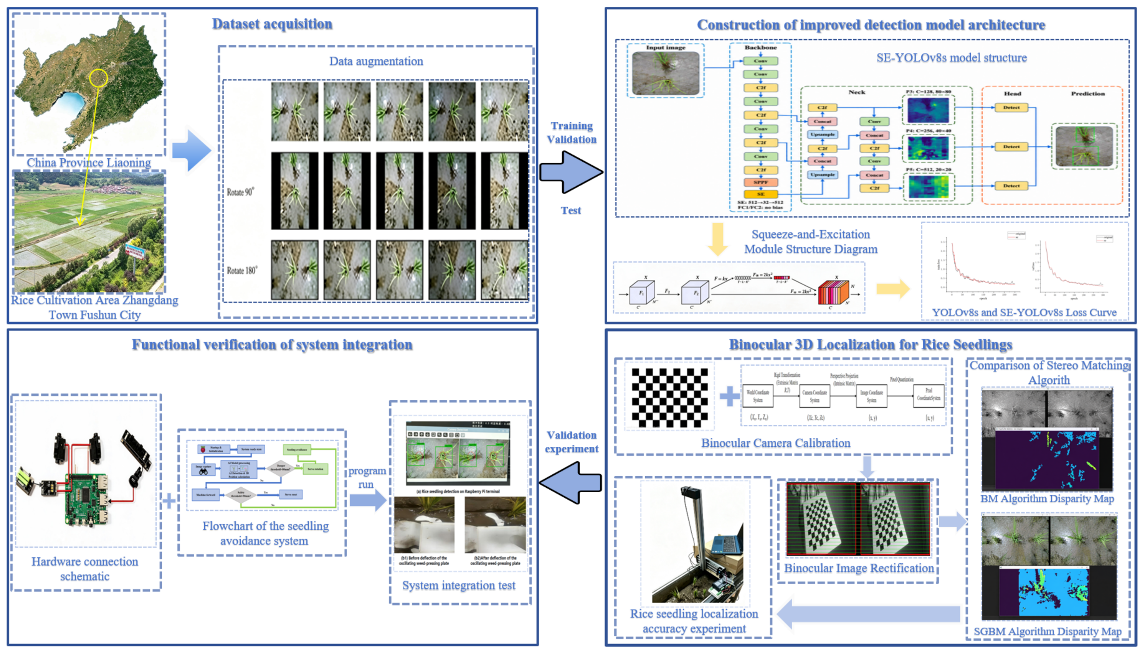
This study investigated rice seedling detection and binocular localization and integrated these functions with a control system on a paddy-field weeding device. The system identifies seedling positions and actuates an avoidance mechanism. The overall workflow of this study is shown in Figure 1.

2.1. Overall Design of the Rice Seedling Localization and Avoidance System

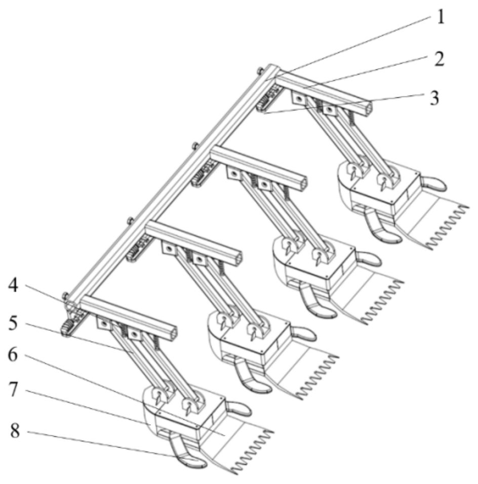
The weeding device mainly consists of binocular cameras, oscillating weed-pressing plates, inter-row grass-pressing plates, and mud guide plates, as shown in Figure 2. The complete device is mounted on a rice transplanter which typically moves continuously along rice rows at 0.3–1.0 m/s.

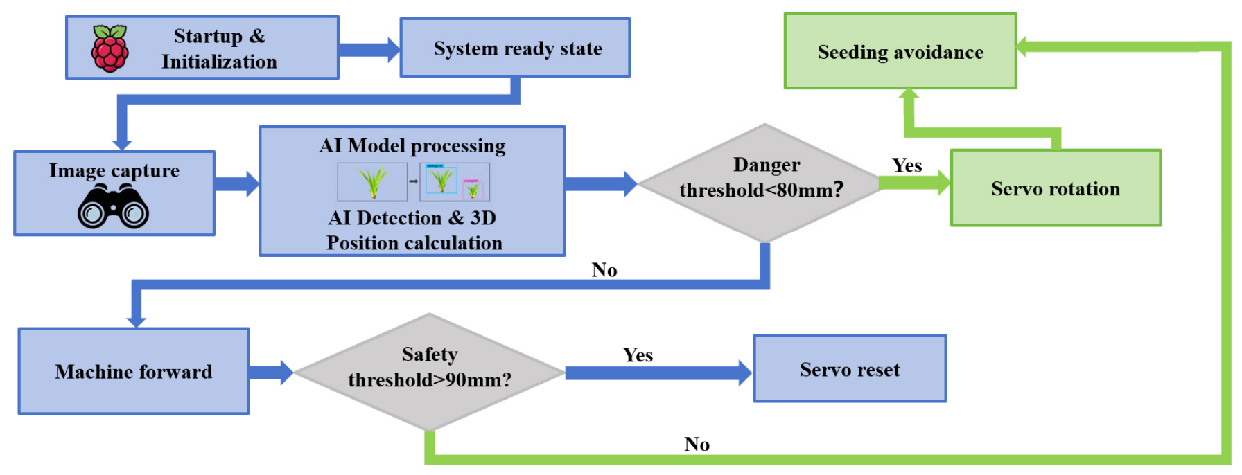
The forward-mounted binocular camera, positioned approximately 650 mm above the ground, continuously captures images of rice seedlings within the working area. The detector identifies rice seedlings, and stereo-matching is used to calculate the spatial coordinates of each seedling center in the camera coordinate system. The Raspberry Pi calculates the forward distance between the oscillating weed-pressing plate and the rice seedling. When this distance falls below a preset threshold, indicating that the seedling has entered the danger zone, the controller outputs a pulse-width modulation (PWM) signal that drives the servo and deflects the plate away from the seedling. Once the weeding component has passed the danger zone, the servo resets and the plate returns to its working position. The cycle repeats as the device travels, allowing continuous weeding with seedling avoidance.

2.2. Rice Seedling Detection Method with Improved YOLOv8s

2.2.1. Data Acquisition

(1)

Image acquisition

Rice seedling images were collected in Zhangdang Town, Dongzhou District, Fushun City, Liaoning Province, China (41°52′–42°02′ N, 124°02′–124°15′ E). The experimental field was planted with Shennong 5588. The dominant weeds were Echinochloa crus-galli and Monochoria vaginalis, with occasional Cyperus difformis. Weed density was low to moderate during image collection.

Images were collected from 10 to 15 July 2025, during the rice tillering stage (BBCH 21–29). Data were collected daily from 09:00 to 12:00 and from 14:00 to 18:00. In total, 800 images at a resolution of 1280 × 720 pixels were collected under sunny (40%; 320 images), cloudy (35%; 280 images), and overcast (25%; 200 images) conditions. These proportions describe the original image collection and do not imply the same distribution within each test subset.

(2)

Data augmentation

To avoid images from the same acquisition sequence or adjacent frames appearing in different subsets, the original images were first grouped by acquisition date and batch, and the training, validation, and test sets were then divided by group. Images from a given batch, including adjacent frames, were assigned to only one subset.

The 800 original images were divided into training, validation and test sets at ratios of 56%, 24%, and 20%, yielding 448, 192, and 160 images, respectively. The ratio of the training set to the validation ratio was 7:3. After the original image dataset was divided, data augmentation was applied separately within the training and validation sets to ensure that no original image or its augmented versions were distributed across different subsets.

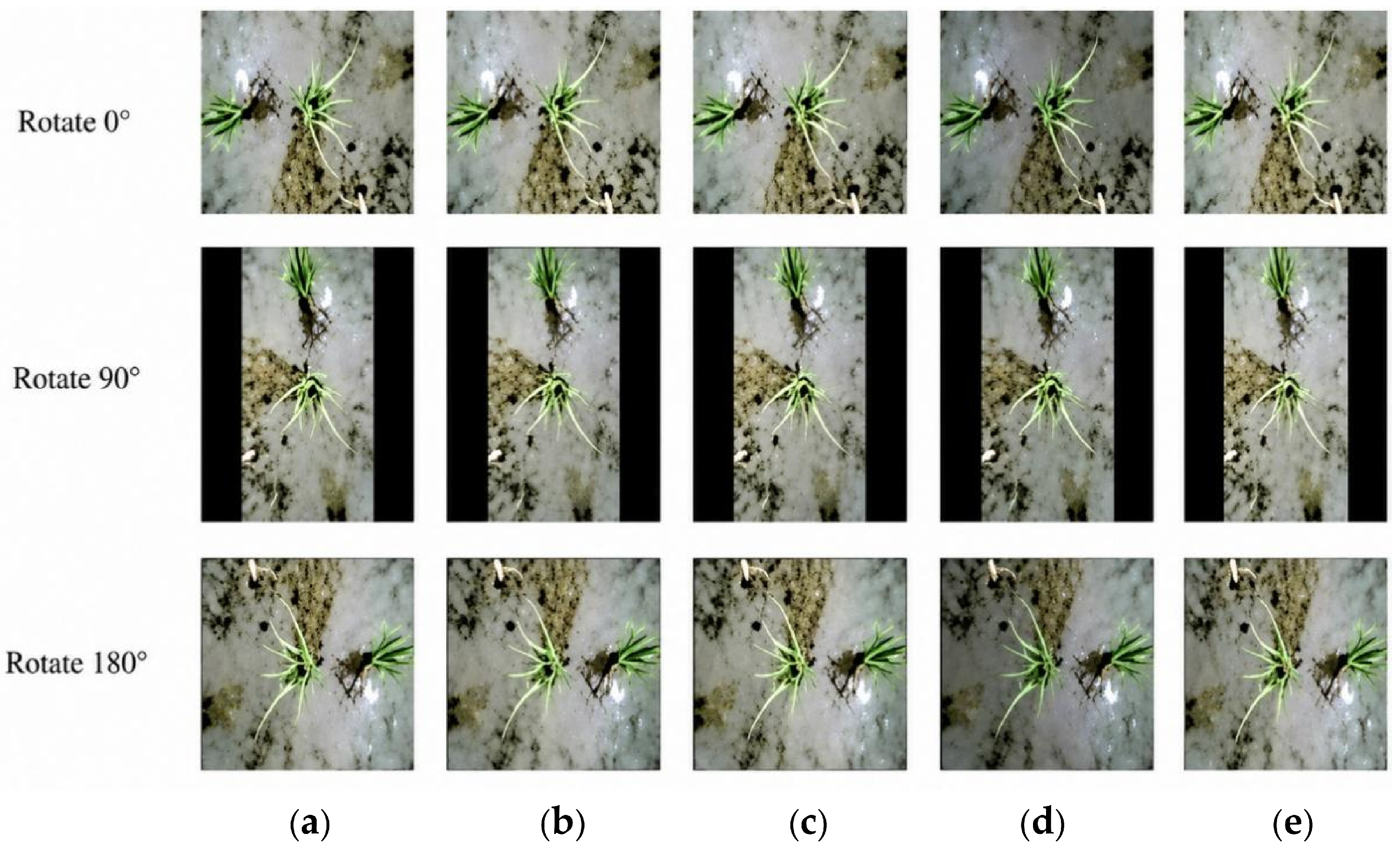
Random augmentations were applied to the images in the training and validation sets using Python 3.10 and OpenCV 4.8, including Gaussian blur, Gaussian noise, gamma correction, and brightness adjustment, to improve the model’s adaptability to illumination and imaging interference in paddy fields. With a threefold expansion, the training set increased from 448 to 1344 images, and the validation set from 192 to 576 images. The test set of 160 images remained unaltered without any augmentation and was used only for final model evaluation. The resulting rice seedling detection dataset comprised 1344 training images, 576 validation images, and 160 independent test images, for a total of 2080 images. Representative augmented images are shown in Figure 3.

(3)

Dataset Creation

Images were annotated manually using LabelImg 1.8.6. The canopy boundary was represented by a rectangular box tightly enclosing the visible leaf expansion area. Targets with partial leaf occlusion but still distinguishable canopy were annotated based on the visible canopy range, and those with severe occlusion that prevented reliable identification of independent canopy boundaries were excluded from valid detection instances. The same annotation criteria were applied across all subsets. The results do not directly represent the detection capability for all severely occluded seedlings.

The training set was used for model parameter learning, the validation set for performance monitoring and model selection during training, and the test set for final performance evaluation. Single-seedling and four-seedling refer to scenarios containing one and four rice seedling targets, respectively.

2.2.2. Construction of the SE-YOLOv8s Detection Model

(1)

SE-YOLOv8s

YOLOv8s was selected as the baseline detector. YOLOv8 consists of a backbone network, a neck network, and a detection head [26,27]. The backbone extracts multi-scale features from the input image, the neck aggregates features across scales, and the detection head classifies objects and regresses their bounding boxes.

Overlapping leaves and interference from water and soil may affect target detection. This study investigated the insertion of an SE channel attention module after the SPPF layer in the YOLOv8s backbone to enhance the selection of informative features. For the ablation study on insertion positions, the compression ratio of SE was fixed at r = 16, and three positions were compared: before SPPF, after SPPF, and at the high-level P5 branch in the Neck. For the comparison of attention modules, the insertion position was fixed after SPPF, and SE was compared with ECA, EMA, CBAM, and Coordinate Attention (CA). All candidate configurations were evaluated under identical data partitioning, input resolution, and training protocols. The SPPF output undergoes multi-scale spatial aggregation; recalibrating channel responses at this stage allows subsequent Neck fusion to leverage the weighted high-level features. This design was evaluated based on the detection results in Section 3.1.2. The comparisons supported placing the SE module after the SPPF in the final SE-YOLOv8s configuration.

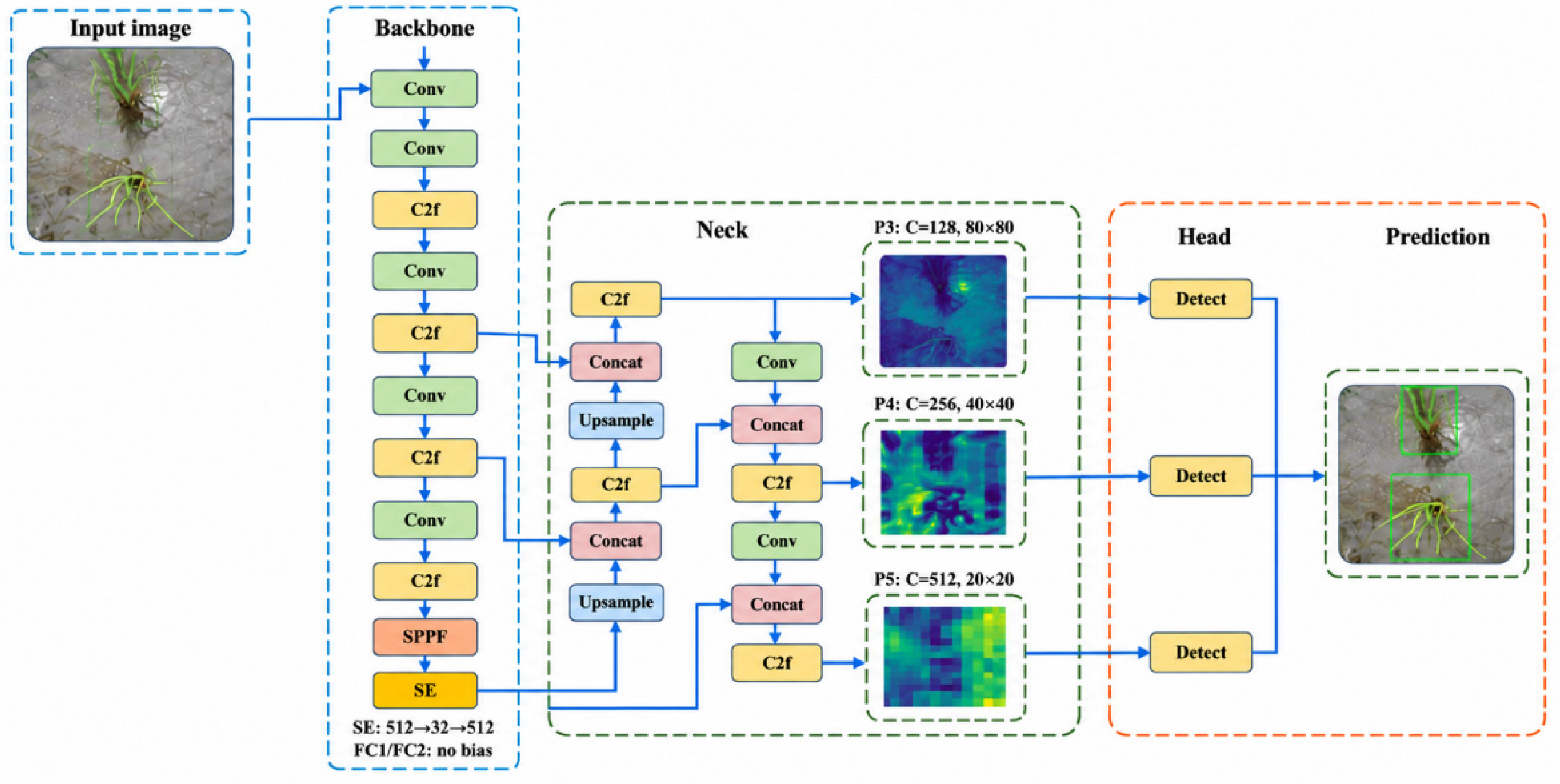
The SE module recalibrates channel-wise feature responses. Figure 4 shows the architecture of SE-YOLOv8s corresponding to the trained weights, where P3, P4, and P5 have 128, 256, and 512 channels, respectively.

The SE module recalibrates channel-wise features in three steps: squeeze, excitation, and scale (Figure 5). Global average pooling first compresses the spatial information of each channel into a channel descriptor vector. Two fully connected layers then model nonlinear dependencies among channels, and a sigmoid function generates the weight for each channel. Finally, these weights are multiplied channel-wise with the original feature map to achieve adaptive recalibration of different channel responses.

An SE channel attention module was inserted after the SPPF output in the YOLOv8s backbone. For a 640 × 640-pixel input, the SPPF output feature map has dimensions of 512 × 20 × 20. With a reduction ratio of 16, the SE module uses two bias-free fully connected layers (512 → 32 → 512), and adds 32,768 trainable parameters.

As shown in

Table 1. Structural characteristics and file sizes of the trained checkpoints.

Item	YOLOv8s	SE-YOLOv8s	Increase
Input size	640 × 640	640 × 640	—
Number of classes	1	1	—
SPPF output	512 × 20 × 20	512 × 20 × 20	—
Attention module	—	SE	+1 SE
SE position	—	After SPPF	—
Reduction ratio	—	r = 16	—
SE channel mapping	—	512 → 32 → 512	—
Params/M	11.136	11.169	+0.033
Params increase/%	—	—	+0.294
GFLOPs (THOP)	28.64696320	28.64743936	+0.00047616
Checkpoint file size/MB, FP32, no optimizer	44.886	45.020	+0.134

Note: GFLOPs were calculated in THOP using the 2 × MAC convention, and exclude the 204,800 element-wise multiplications in the SE gating operations. Both files were saved in FP32 with identical fields and without optimizer states.

, with single-class detection, 640 × 640 input resolution, and no network fusion, the parameter counts of YOLOv8s and SE-YOLOv8s were verified as 11,135,987 and 11,168,755, respectively, with a parameter increase of approximately 0.294%. The weights correspond to epoch 300 and random seed 42 and were generated using Ultralytics 8.3.89.

(2)

Model Training Environment and Parameter Settings

Model training was performed with PyTorch 2024.2 on a computer running Windows 11 and equipped with an Intel i7-13620 processor and an NVIDIA RTX 4060 GPU with 8 GB of memory. The software environment included CUDA 11.8, Python 3.8, and Ultralytics YOLOv8 (version 8.0.x). The model was initialized with COCO-pretrained weights. The input resolution was 640 × 640 pixels, the initial learning rate was 0.01, the weight decay coefficient was 0.0005, batch size was 24, and training continued for 300 epochs. The SGD optimizer (momentum = 0.937) and cosine annealing scheduler (warmup epochs = 3) were used. No early stopping was applied, and the random seed was 42.

2.3. Method of Binocular Localization for Rice Seedlings

2.3.1. Binocular Camera Calibration and Image Rectification

A binocular camera with approximately parallel optical axes was used for localization. It was mounted 650 mm above the ground to provide an adequate field of view while maintaining sufficient image resolution for seedlings. Its principal specifications are listed in

Table 2. Specifications of the binocular camera.

Item	Specification
Data interface	USB 3.0 interface
Communication protocol	UVC (USB Video Class), plug-and-play
Supported platforms	Windows, Linux, ROS, iOS, Android, etc.
Data output format	YUY2
Resolution	2560 × 720, 1280 × 640, 640 × 240
Frame rate	30 FPS

.

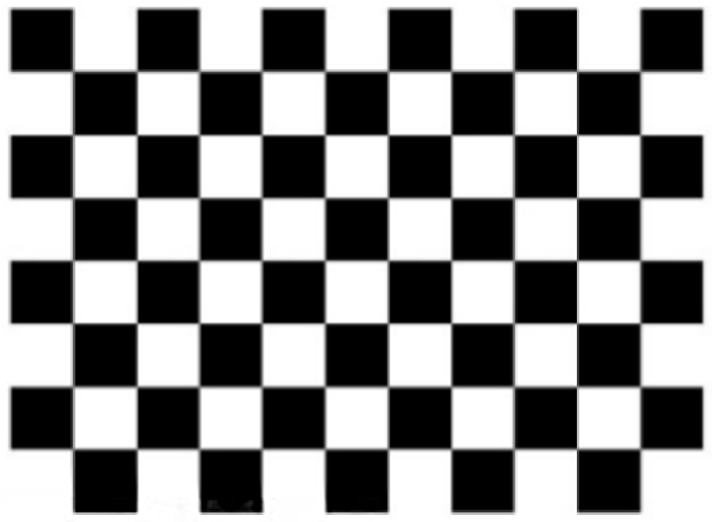
Camera calibration is fundamental to binocular localization. The binocular camera was calibrated using Zhang’s method [28] in the MATLAB R2024b Stereo Camera Calibrator toolbox. The calibration target was an 8 × 11 checkerboard (i.e., 7 × 10 internal corner points) with a square size of 27 mm (Figure 6). Twenty stereo image pairs were acquired under natural lighting while the target was rotated and translated through various poses, covering distances of approximately 30–80 cm from the cameras, with pitch angles of ±30°, yaw angles of ±45°, and roll angles of ±20°. Image pairs with a reprojection error exceeding 0.5 pixel were discarded; the number of pairs retained after this screening is reported in Section 3.2.1. The remaining images were used to estimate the intrinsic parameters, distortion coefficients, rotation matrix, and translation vector of the stereo camera pair.

Manufacturing and assembly tolerances prevent the two camera optical axes from remaining perfectly parallel. Epipolar rectification was therefore applied to reduce vertical disparity. In contrast to Hartley’s uncalibrated approach, Bouguet rectification uses the estimated stereo geometry to transform the left and right images so that corresponding epipolar lines are horizontally aligned [29]. This reduces the stereo-matching search from two dimensions to one and was therefore adopted in this study.

2.3.2. Coordinate System Transformation

To convert the pixel coordinates of a rice seedling into spatial coordinates, relationships among the pixel, image, camera, and world coordinate systems were defined using the pinhole camera model, as shown in Figure 7.

The origin of the camera coordinate system was defined at the optical center of the left camera. The Z-axis followed the camera’s optical axis; because the camera pointed vertically downward, this axis corresponded to the vertical direction. The X-axes and Y-axes were located in the plane perpendicular to the optical axis, with the Y-axis along the forward direction of the weeding device, and the X-axis in the lateral direction. The correspondence between the camera coordinate system and the test bench coordinate system was used to interpret the displacement measurement results in each direction. In the following sections, “forward distance” refers to the distance along the Y-axis.

For a spatial point P with camera coordinates (X_c, Y_c, Z_c) in the camera coordinate system, its projection onto the image plane is given by (x, y) in Equation (1). The pinhole imaging relationship is as follows:

$$s\left[\begin{array}{c}x\\ y\\ 1\end{array}\right]=\left[\begin{array}{ccc}{f}_x& 0& u_0\\ 0& f_y& v_0\\ 0& 0& 1\end{array}\right]\left[\begin{array}{c}{X}_c\\ Y_c\\ Z_c\end{array}\right]$$

(1)

where s is the scale factor, f_x and f_y are the equivalent camera focal lengths of the camera, and (u₀, v₀) is the coordinate of the image principal point.

A rigid-body transformation comprising a rotation matrix R and a translation vector T maps the world coordinate system to the camera coordinate system. The resulting camera coordinates are then projected onto the image plane and converted to pixel coordinates. The complete projection from a world point (X_w, Y_w, Z_w) to its corresponding pixel coordinates (u, v) is expressed as follows:

$$Z_c\left[\begin{array}{c}u\\ v\\ 1\end{array}\right]=\left[\begin{array}{ccc}{f}_x& 0& u_0\\ 0& f_y& v_0\\ 0& 0& 1\end{array}\right]\left[\begin{array}{cc}R& T\\ 0& 1\end{array}\right]\left[\begin{array}{c}{X}_{\omega }\\ Y_{\omega }\\ Z_{\omega }\\ 1\end{array}\right]=M_1{M}_2\left[\begin{array}{c}{X}_{\omega }\\ Y_{\omega }\\ Z_{\omega }\\ 1\end{array}\right]$$

(2)

where Z_c is the spatial distance from the target point to the camera, R is the rotation matrix, T is the translation vector, M₁ is the intrinsic matrix, and M₂ is the extrinsic matrix.

2.3.3. Selection of Stereo Matching Algorithm

Depth estimation requires a stereo-matching algorithm that balances computational efficiency and robustness. Stereo-matching methods can be categorized as local, global, or semi-global according to their optimization scope [30]. Local methods are computationally efficient but can be sensitive to illumination variation, muddy water, and reflections in paddy fields. Global methods can improve accuracy but generally require greater computational resources. Semi-global methods offer a compromise between these two approaches and are therefore suitable for real-time field use.

Block matching (BM), a local method, and semi-global block matching (SGBM) were compared using binocular images of rice seedlings. The quality of their disparity maps and their computational cost were evaluated, and SGBM was selected to generate disparity maps for subsequent spatial coordinate computation of rice canopy visual reference points.

2.3.4. Localization of Rice Seedling Centers

The SGBM algorithm was used to compute the disparity maps of the rectified left and right images, and SE-YOLOv8s was used to obtain the rice canopy detection boxes, after binocular camera calibration and image rectification. The center of each detection box was used as the sampling point for the disparity value. Because SGBM disparity maps contain invalid (hole) pixels, particularly in low-texture regions such as canopy centers, the disparity assigned to a detection was taken as the median of the valid disparity values within a 5 × 5 pixel window centered on the box center. If the window contained no valid disparity, the target was treated as having no reliable depth: it was not used for the avoidance decision in that frame, but it was still counted in the detection evaluation. Target disparity was obtained from the SGBM disparity map, not from the horizontal offset between the left and right box centers. Subsequently, the target disparity was converted into the spatial coordinates of the canopy visual reference point using the camera calibration parameters.

The detection-box center was used as the visual localization reference point for rice seedlings. A protection zone with a radius of 50 mm was defined for seedling avoidance control to provide space for the reference point deviation and other localization errors. Although the reference-point displacement was smaller than the protection zone radius, it still caused the protection zone to deviate from the stem base, and its influence cannot be ignored. The localization experiment evaluated the coordinate variation error of the visual reference point, while the actual coverage of the protection zone over the stem base still requires further verification.

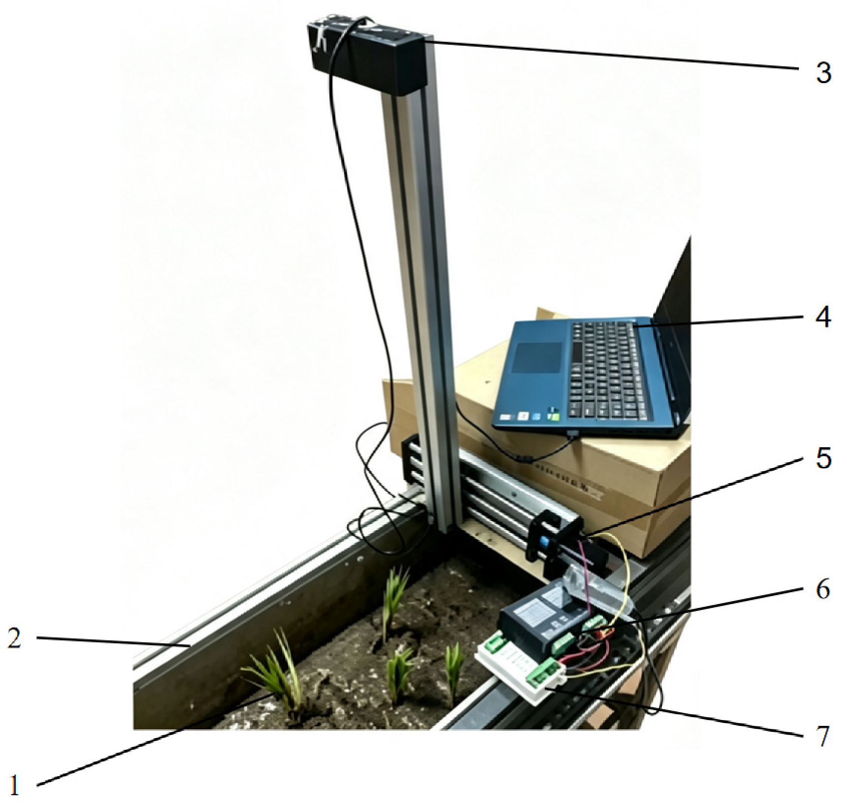
A test platform comprising an electronically controlled translation stage, the binocular camera, and rice seedling samples was constructed to assess localization accuracy (Figure 8). The binocular camera was mounted vertically at a working height of 650 mm. Because the avoidance mechanism moves primarily in a plane, localization accuracy was evaluated along the X- and Y-axes.

2.4. Seedling-Avoidance Control System

2.4.1. Hardware Design

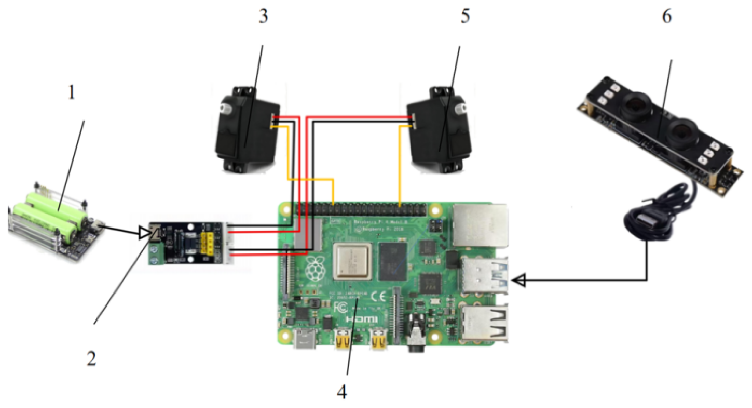
The seedling-avoidance control system comprises a Raspberry Pi 4B, a binocular vision module, a ZP20S bus digital servo, and a voltage regulator (Figure 9). The Raspberry Pi is powered through a Type-C interface at 5 V and 3 A and supplies power to the binocular vision module. The servo is powered independently by a portable power source through the voltage regulation module at 5–9 V. The binocular vision module communicates with the Raspberry Pi through USB and the servo is connected through a hardware PWM-capable general-purpose input/output interface. Servo pulse widths of 0.5–2.5 ms correspond to angular positions of 0–180°. The initial angle of the oscillating weed-pressing plate was set to 0°, and the avoidance angle to 90°. The Raspberry Pi 4B coordinates image acquisition, rice seedling detection, coordinate calculation, and servo actuation.

2.4.2. Seedling-Avoidance- Control Process

At startup, the Raspberry Pi 4B initializes the servos and binocular camera, loads the SE-YOLOv8s model, and imports the operating and calibration parameters. The acquired stereo images are rectified before SE-YOLOv8s detects the rice seedlings and returns the pixel coordinates of the detection-box centers. Binocular localization converts these pixel coordinates into seedling coordinates in the camera reference frame. The fixed position of the oscillating weed-pressing plate’s rotation axis in this frame provides a reference for avoidance-distance calculations.

A threshold-based state machine controls the servo according to the seedling position relative to the plate’s rotation axis. When the forward distance from a valid seedling target to the reference point decreases to 80 mm or less, the controller changes from normal operation to avoidance and rotates the servo to 90°. Once the device passes the seedling and the rearward distance reaches 90 mm, the controller enters the reset state and returns the servo to 0°. These thresholds were based on the dimensions and range of the oscillating weed-pressing plate. The complete control workflow is shown in Figure 10.

2.5. Experimental Design and Evaluation Metrics

2.5.1. Experimental Design

The rice seedling detection and localization system was evaluated through the following comparison and validation experiments.

(1)

Attention configuration evaluation

To analyze the influence of SE-YOLOv8s on detection performance, two sets of experiments were conducted under consistent conditions, including dataset partitioning, input resolution, initialization, optimizer, and number of training epochs.

①

Ablation study on SE insertion position

The SE compression ratio was fixed at 16. Four configurations were compared: a YOLOv8s baseline without the attention module, and three improved configurations with SE inserted before SPPF, after SPPF, or at the high-level P5 feature branch in the neck. Each configuration was trained independently three times with random seeds 42, 43, and 44, yielding 12 runs in total.

②

Comparison of different attention mechanisms

SE, ECA, EMA, CBAM, and CA were inserted after SPPF to evaluate their detection performance under otherwise identical experimental conditions. Each attention configuration was trained once independently. The results of the two sets of experiments are presented for both single-seedling and four-seedling scenarios. These results support descriptive comparisons among the configurations; no statistical significance is inferred from them.

(2)

Comparison with representative detection models

SE-YOLOv8s was compared with Faster R-CNN, YOLOv5s, YOLOv7-tiny, and the original YOLOv8s. ResNet-50 was used as the Faster R-CNN backbone. Except for the architecture-specific configurations of each model, all models used the same dataset partitioning, input image size, number of training epochs, and test sets, and were evaluated under a unified evaluation pipeline. The test sets were evaluated separately for single-seedling and four-seedling scenarios. YOLOv8s and SE-YOLOv8s were trained independently five times, while Faster R-CNN, YOLOv5s, and YOLOv7-tiny were trained once. All models report precision, recall, F1, AP50, AP75, and AP50-95, along with parameter count, FLOPs, and frames per second (FPS), to ensure comparisons under identical test scenarios and evaluation metrics.

(3)

Rice seedling localization experiment

The binocular camera was mounted vertically downward on the test bench at a height of approximately 650 mm. The translation stage moved the camera diagonally at 45° to the X-axis, producing displacement components of approximately 60 mm in both the X and Y directions. The stage’s rated positioning accuracy was ±0.01 mm. Localization error was calculated by comparing the visually measured coordinate changes along each direction with the known displacements. Eight stage positions were tested, with five replicate measurements at each position, and the mean of the five measurements was used as the localization error rate for that position.

2.5.2. Detection Evaluation Metrics

Detection performance was evaluated using precision, recall, F1, AP50, AP75, and AP50-95. Computational and deployment characteristics were evaluated using FPS, parameter count, floating-point operations (FLOPs), and model size. FPS was measured on an RTX 4060 with a batch size of 1, including preprocessing and postprocessing, and averaged over multiple runs. F1 is the harmonic mean of precision and recall and was uniformly calculated as F1 = 2PR/(P + R).

Since the subsequent binocular localization uses the center coordinates of the rice seedling detection boxes as visual input, deviations in predicted box positions may further affect center point extraction and spatial localization. Therefore, in addition to AP50, AP75 and AP50-95 are also adopted to evaluate the box localization performance of different detection models. It should be noted that high-IoU metrics are used to reflect the consistency of predicted box localization at the detection stage; the final spatial localization accuracy is independently evaluated through the binocular localization experiments in Section 3.2.

2.5.3. Rice Seedling Localization Evaluation Metrics

Mean relative localization errors along the X- and Y-axes were used to evaluate the binocular system. For each axis, the estimated change in seedling position before and after camera translation was compared with the measured stage displacement. Relative localization error e was calculated as follows:

$$e=\left|{\displaystyle \frac{|W_1-W_0|-S}{S}}\right|\times 100\%$$

(3)

where W₀ and W₁ are the seedling-center coordinates before and after camera translation, respectively (mm), and S is the nominal camera displacement along the corresponding axis (S = 60 mm in this experiment).

The mean relative localization errors along X and Y directions were calculated as follows:

$${\overline{e}}_X={\displaystyle \frac{1}{\mathrm{n}}}{\displaystyle {\sum }_{i=1}^n{e}_{X,i}}$$

(4)

$${\overline{e}}_Y={\displaystyle \frac{1}{\mathrm{n}}}{\displaystyle {\sum }_{i=1}^n{e}_{Y,i}}$$

(5)

where n is the number of test positions (n = 8); e_X,i is the X-direction- error rate for the ith sample; and e_Y,j is the Y-direction- error rate for the ith sample.

The mean coordinates from the five repeated measurements at each position were used to calculate the displacement and error rate for that position. The standard deviation at each position was calculated from the error rates of the five replicates.

3. Results and Analysis

3.1. Rice Seedling Detection Results

3.1.1. Model Training and Convergence

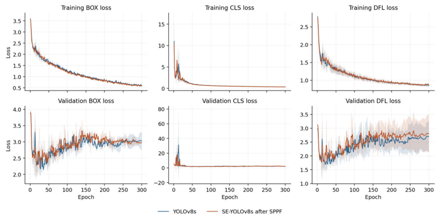
Figure 11 shows the training and validation loss curves of YOLOv8s and SE-YOLOv8s across three independent runs with random seeds 42, 43, and 44. Solid lines show the mean loss at each epoch, and the shaded areas show the sample standard deviation, with no smoothing applied. The training losses of these two models initially decreased but subsequently rose and fluctuated more widely, suggesting instability in the small validation set. These curves do not establish faster convergence or better generalization for SE-YOLOv8s and do not depict variation in the main experiments.

3.1.2. Ablation Study on the SE Modules

(1)

Ablation study on SE insertion positions

Table 3. Detection performance of the SE module at different insertion positions in SPPF.

Model/Position	Scenario	P/%	R/%	F1/%	AP50/%	AP75/%	AP50-95/%
YOLOv8s	Single	92.3	91.7	92.0	94.9	84.6	67.9
SE/SPPF-before	Single	94.0	94.4	94.2	97.1	87.8	70.4
SE/SPPF-after	Single	94.6	95.2	94.9	97.8	88.9	71.3
SE/Neck P5	Single	93.5	93.9	93.7	96.4	86.9	69.5
YOLOv8s	Four	89.7	89.3	89.5	92.4	82.1	64.8
SE/SPPF-before	Four	92.0	92.7	92.3	95.2	85.5	67.6
SE/SPPF-after	Four	92.8	93.5	93.1	96.1	86.5	68.6
SE/Neck P5	Four	91.5	92.0	91.7	94.6	84.8	66.8

Note: Single and Four denote the single-seedling and four-seedling scenarios, respectively. The SE compression ratio was fixed at 16; values are the means of three independent training runs with random seeds 42, 43, and 44.

compares the detection performance of the SE module at different insertion positions around the SPPF layer. With the SE structure and compression ratio fixed at 16, the detection metrics of YOLOv8s with the SE module inserted at different positions were all higher than those of the YOLOv8s baseline. The SPPF-after position achieved AP50 of 97.8% and 96.1% in the single-seedling and four-seedling scenarios, respectively, which were 0.7 and 0.9 percentage points higher than those at the SPPF-before position and 1.4 and 1.5 percentage points higher than those at the Neck P5 position. The AP50-95 reached 71.3% and 68.6%, respectively, also higher than the other two positions. These results indicate that under the same SE structure and training conditions, the insertion position of the SE module affects the detection performance, and the SPPF-after position achieves the best performance in both test scenarios. After multi-scale spatial feature aggregation by SPPF, the SE module recalibrates the high-level semantic features through channel-wise weighting and passes the enhanced features to the Neck for subsequent multi-scale fusion, which is beneficial for improving the representation of informative seedling features. Based on the ablation results and the network structural characteristics, the SPPF-after position was selected as the insertion location for the SE module.

(2)

Comparison of different attention mechanisms

Table 4. Detection performance of different attention mechanisms.

Model	Scenario	P/%	R/%	F1/%	AP50/%	AP75/%	AP50-95/%
YOLOv8s	Single	92.3	91.7	92.0	94.9	84.6	67.9
SE-YOLOv8s	Single	94.6	95.2	94.9	97.8	88.9	71.3
ECA-YOLOv8s	Single	92.1	94.7	93.4	97.2	88.1	70.9
EMA-YOLOv8s	Single	93.8	94.5	94.1	97.0	87.7	70.6
CBAM-YOLOv8s	Single	90.9	92.8	91.8	94.3	85.0	68.3
CA-YOLOv8s	Single	91.8	90.3	91.0	93.9	83.8	67.2
YOLOv8s	Four	89.7	89.3	89.5	92.4	82.1	64.8
SE-YOLOv8s	Four	92.8	93.5	93.1	96.1	86.5	68.6
ECA-YOLOv8s	Four	89.4	92.6	91.0	95.4	85.7	68.2
EMA-YOLOv8s	Four	91.5	92.1	91.8	95.1	85.2	67.9
CBAM-YOLOv8s	Four	88.1	90.5	89.3	91.8	81.5	65.3
CA-YOLOv8s	Four	89.3	87.0	88.1	91.2	80.4	64.0

Note: Each attention configuration was trained once independently.

shows that different attention mechanisms exhibited varying detection performance in rice seedling detection. SE-YOLOv8s obtained the highest values of the reported detection metrics in both single-seedling and four-seedling scenarios. In the single-seedling scenario, its AP50, AP75, and AP50-95 reached 97.8%, 88.9%, and 71.3%, respectively; in the four-seedling scenario, they reached 96.1%, 86.5%, and 68.6%, respectively. ECA-YOLOv8s and EMA-YOLOv8s achieved performance close to that of SE-YOLOv8s. Specifically, ECA-YOLOv8s achieved AP50 of 97.2% and 95.4% in the single-seedling and four-seedling scenarios, which were only 0.6 and 0.7 percentage points lower than SE-YOLOv8s, and its AP50-95 was 0.4 percentage points lower in both scenarios. EMA-YOLOv8s also achieved good overall performance, but was slightly inferior to SE and ECA in AP50, AP75, and AP50-95. In contrast, CBAM and CA showed unstable improvements on some metrics, indicating that different attention mechanisms have different effects on feature representation of rice seedlings. Because each attention configuration was trained only once, these differences are descriptive rather than statistically supported; the margins of SE over ECA (0.6 and 0.7 percentage points in AP50, and 0.4 percentage points in AP50-95) are comparable to the run-to-run variation reported in

Table 5. Performance comparison of YOLOv8s and SE-YOLOv8s.

Model	Scene	P/%	R/%	mAP@0.5/%	mAP@0.5:0.95/%	AP75/%	F1/%	Params/M	GFLOPs	FPS	Size/MB
YOLOv8s	Single	92.3 ± 1.7	92.0 ± 4.8	94.9 ± 1.8	67.9 ± 3.5	84.6 ± 2.5	92.1 ± 2.8	11.136	28.6470	29.3	44.886
YOLOv8s	Four	89.7 ± 1.9	90.3 ± 3.8	92.4 ± 2.2	64.8 ± 3.3	82.1 ± 2.3	89.9 ± 2.0	11.136	28.6470	27.1	44.886
SE-YOLOv8s	Single	94.5 ± 1.3	94.9 ± 2.2	97.8 ± 1.2	71.3 ± 1.9	88.9 ± 2.5	94.7 ± 1.0	11.169	28.6474	29.8	45.020
SE-YOLOv8s	Four	92.8 ± 1.3	92.0 ± 3.0	96.1 ± 2.2	68.6 ± 3.4	86.5 ± 2.3	92.4 ± 1.8	11.169	28.6474	28.8	45.020

Note: FPS was measured on a PC platform. All values are presented as mean ± standard deviation (n = 5).

, where the standard deviation of recall reached 4.8 percentage points. Overall, SE performed comparably to, and marginally above, ECA under this single-run comparison, and the SE attention mechanism demonstrated good applicability on the current dataset and network structure. Combined with the insertion position ablation results, the SE-YOLOv8s architecture with the SE module embedded after SPPF was finally adopted.

(3)

Analysis of the SE compression ratio

The effects of the SE reduction ratio on parameter count were calculated theoretically for r = 8, 16, and 32, with C = 512 input channels and no bias terms in the two fully connected layers. The intermediate channel number is C/r, and the additional parameters introduced by the SE module are ΔN = 2C²/r. The parameter increases for the three settings are 65,536, 32,768, and 16,384, respectively (

Table 6. Parameter counts of the SE module at different compression ratios.

SE Compression Ratio r	Intermediate Channels C/r	Additional Weight Parameters
8	64	65,536
16	32	32,768
32	16	16,384

Note: C = 512 input channels, no bias in fully connected layers.

).

(4)

Performance comparison of YOLOv8s and SE-YOLOv8s

The detection performance of YOLOv8s and SE-YOLOv8s in single-seedling and four-seedling scenarios is presented in Table 5.

In the single-seedling scenario, SE-YOLOv8s achieved a precision of 94.5 ± 1.3%, recall of 94.9 ± 2.2%, mAP@0.5 of 97.8 ± 1.2%, and F1-score of 94.7 ± 1.0%. These values exceeded those of YOLOv8s by 2.2, 2.9, 2.9, and 2.6 percentage points, respectively. The mAP@0.5:0.95 was 71.3 ± 1.9%, 3.4 percentage points higher than the baseline value of 67.9 ± 3.5%, and AP@0.75 was 88.9 ± 2.5%, 4.3 percentage points higher than the baseline value of 84.6 ± 2.5%. These results indicate that the SE module improved both detection sensitivity and localization performance on this test set.

In the four-seedling scenario, SE-YOLOv8s achieved a precision of 92.8 ± 1.3%, recall of 92.0 ± 3%, mAP@0.5 of 96.1 ± 2.2%, and F1-score of 92.4 ± 1.8%, exceeding the corresponding YOLOv8s values by 3.1, 1.7, 3.7, and 2.5 percentage points, respectively. The mAP@0.5:0.95 and AP@0.75 were 68.6 ± 3.4% and 86.5 ± 2.3%, respectively, representing increases of 3.8 and 4.4 percentage points over the baseline. The performance was lower than in the single-seedling scenario, which is consistent with the greater leaf overlap and boundary ambiguity in images containing four seedlings.

On the PC platform, SE-YOLOv8s processed the single-seedling and four-seedling scenarios at 29.8 and 28.8 FPS, respectively, which were 0.5 and 1.7 FPS higher than those of YOLOv8s. The parameter counts, GFLOPs, and file sizes were calculated consistently across models as described for Table 1, with weights saved in FP32 format and without optimizer states. These FPS results do not represent the processing speed on the Raspberry Pi platform.

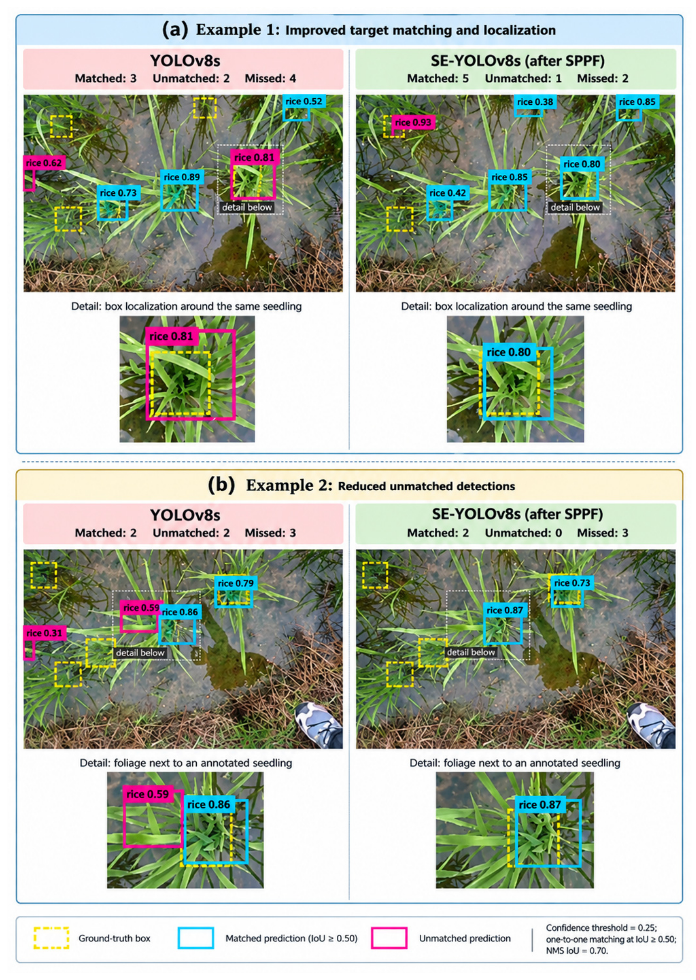
Paired t-tests were performed on the five independent runs for each metric. In the single-seedling scenario, the improvements in mAP@0.5 (p = 0.015) and precision (p = 0.046) were statistically significant (p < 0.05), while the improvement in recall (p = 0.089) was not statistically significant. In the four-seedling scenario, the improvement in mAP@0.5 (p = 0.009) was statistically significant (p < 0.05), while the improvements in precision (p = 0.087) and recall (p = 0.071) were not statistically significant. Typical rice images with leaf overlap, water surface background, and local target interference were selected for qualitative comparison, as shown in Figure 12, to further visually analyze the detection differences before and after the introduction of the SE module.

Figure 12 presents typical detection results of YOLOv8s and SE-YOLOv8s on the same rice images. The yellow dashed boxes indicate the ground-truth annotations, the blue solid boxes indicate the predicted boxes that successfully match the ground-truth targets, and the pink solid boxes indicate the unmatched predictions.

In Example 1, YOLOv8s successfully matched 3 targets, with 2 unmatched predictions and 4 missed detections. SE-YOLOv8s successfully matched 5 targets, with unmatched predictions reduced to 1 and missed detections reduced to 2. The zoomed-in views show that for the same seedling with obvious leaf overlap, SE-YOLOv8s achieved better alignment between the predicted boxes and the ground-truth annotations.

In Example 2, both models successfully matched 2 targets, but YOLOv8s generated 2 unmatched predictions, while SE-YOLOv8s generated none. The zoomed-in views show that YOLOv8s generated extra detections around the leaf regions near the targets, whereas SE-YOLOv8s reduced such interference.

Therefore, the introduction of the SE module improved overall detection metrics, including precision, recall, and AP, and achieved better detection and localization performance under leaf overlap and complex water surface conditions, while reducing false positives in background regions.

3.1.3. Comparison with Representative Detection Models

To further evaluate the comprehensive performance of SE-YOLOv8s, it was compared with Faster R-CNN, YOLOv5s, and YOLOv7-tiny under identical data partitioning, input resolution, and test protocols. The results are shown in

Table 7. SE-YOLOv8s compared with representative detection models.

Model	Scene	P/%	R/%	mAP@0.5/%	mAP@0.5:0.95/%	AP75/%	F1/%	Params/M	GFLOPs	FPS	Size/MB
Faster R-CNN	Single	90.1	87.1	90.2	62.6	77.8	88.6	44.5	128.0	12.3	179.4
Faster R-CNN	Four	88.0	84.3	88.2	59.9	75.6	86.1	44.5	128.0	11.6	179.4
YOLOv5s	Single	93.1	90	94.1	67.0	83.4	91.5	7.2	15.8	28.8	29.0
YOLOv5s	Four	90.9	88.6	92.0	64.2	81.1	89.7	7.2	15.8	27.2	29.0
YOLOv7-tiny	Single	90.7	88.6	92.7	65.4	81.4	89.6	6.1	13.2	29.5	24.6
YOLOv7-tiny	Four	88.6	87.1	90.7	62.6	79.1	87.8	6.1	13.2	27.9	24.6

Note: FPS values were recorded on a PC platform.

. YOLOv8s results are given in Table 5 and are therefore not repeated here.

Table 7 shows that SE-YOLOv8s achieved the highest detection metrics among all compared models in both single-seedling and four-seedling scenarios. In the single-seedling scenario, its precision of 94.5% exceeded those of Faster R-CNN, YOLOv5s, and YOLOv7-tiny by 4.4, 1.4, and 3.8 percentage points, respectively. Its recall of 94.9% exceeded the corresponding values by 7.8, 4.9, and 6.3 percentage points. Its mAP@0.5 of 97.8% was 7.6, 3.7, and 5.1 percentage points higher. The above comparisons are based on the test conditions of this study.

In the four-seedling scenario, SE-YOLOv8s achieved an mAP@0.5 of 96.1%, 7.9, 4.1, and 5.4 percentage points higher than Faster R-CNN, YOLOv5s, and YOLOv7-tiny, respectively. Its mAP@0.5:0.95 was 68.6%, 8.7, 4.4, and 6.0 percentage points higher, and its AP75 was 86.5%, 10.9, 5.4, and 7.4 percentage points higher. These results indicate that SE-YOLOv8s achieved better detection and localization performance among the compared models under the tested scenarios.

In terms of resource metrics, SE-YOLOv8s has 11.169 M parameters, 28.6474 GFLOPs, and a weight file size of 45.020 MB in FP32 precision. Compared to YOLOv8s, it introduces 32,768 additional parameters, with an increase of approximately 0.294%. Its computational cost is lower than that of Faster R-CNN (128.0 GFLOPs), but higher than those of YOLOv5s (15.8 GFLOPs) and YOLOv7-tiny (13.2 GFLOPs). SE-YOLOv8s achieved 29.8 and 28.8 FPS on the PC platform in the single-seedling and four-seedling scenarios, respectively, which were 0.5 and 1.7 FPS higher than YOLOv8s, and 0.3 and 0.9 FPS higher than YOLOv7-tiny. These FPS values were measured only on a PC platform and do not represent the actual processing performance on the Raspberry Pi.

3.2. Binocular Localization Results

3.2.1. Binocular Camera Calibration

After calibrating the left and right cameras individually, stereo calibration was performed to estimate their relative pose. The resulting rotation matrix R and translation vector T define the transformation between the two camera frames.

The intrinsic parameter matrix of the left camera (unit: pixels) is:

$$K_{\mathrm{L}}=\left[\begin{array}{ccc}724.560019770400& 0& 677.443502284479\\ 0& 728.971881836387& 330.723878280721\\ 0& 0& 1\end{array}\right]$$

The distortion coefficients of the left camera are:

D₁ = [0.08995 − 0.05999 − 0.006572 − 0.003377]

The intrinsic parameter matrix of the right camera (unit: pixels) is:

$$K_{\mathrm{R}}=\left[\begin{array}{ccc}728.078680056073& 0& 651.539975382766\\ 0& 732.492613505916& 338.734577633455\\ 0& 0& 1\end{array}\right]$$

The distortion coefficients of the right camera are:

D₂ = [0.09152 − 0.063879 − 0.003880 − 0.004867]

The rotation matrix R of the binocular system is:

$$R=\left[\begin{array}{ccc}0.99989& 0.000446& -0.004637\\ -0.000477& 0.999978& -0.006526\\ 0.004634& 0.006528& 0.999967\end{array}\right]$$

The translation vector T is:

$$T=\left[\begin{array}{ccc}60.060661& 0.073758& 0.584825\end{array}\right]$$

In the coordinate transformation, M₁ and M₂ denote the intrinsic and extrinsic matrices of the general pinhole model; therefore, the left and right intrinsic matrices are denoted K_L and K_R. The calibrated values are reported in the order (f_x, f_y, c_x, c_y) returned by the calibration toolbox. The equivalent focal lengths are (724.56, 728.97) px for the left camera and (728.08, 732.49) px for the right camera, and the principal points are (677.44, 330.72) px and (651.54, 338.73) px, respectively. The calibration used the 20 checkerboard image pairs that passed the screening described in Section 2.3.1. No pair exceeded the 0.5-pixel reprojection-error threshold, so all 20 acquired pairs were retained. The reprojection errors of the left and right cameras were 0.33 and 0.37 pixels, respectively, and the mean epipolar error after rectification was 0.31 pixels. Rectification substantially reduced the vertical-coordinate differences between corresponding points. The calibrated baseline was 60.06066 mm, and the external housing width measured with a vernier caliper was 60.03 mm, a difference of 0.03066 mm (approximately 0.05%). Because a caliper measures an external housing dimension, not the separation between the two optical centers, this agreement is a consistency check of the physical assembly and not an independent validation of the calibration accuracy.

3.2.2. Binocular Image Rectification

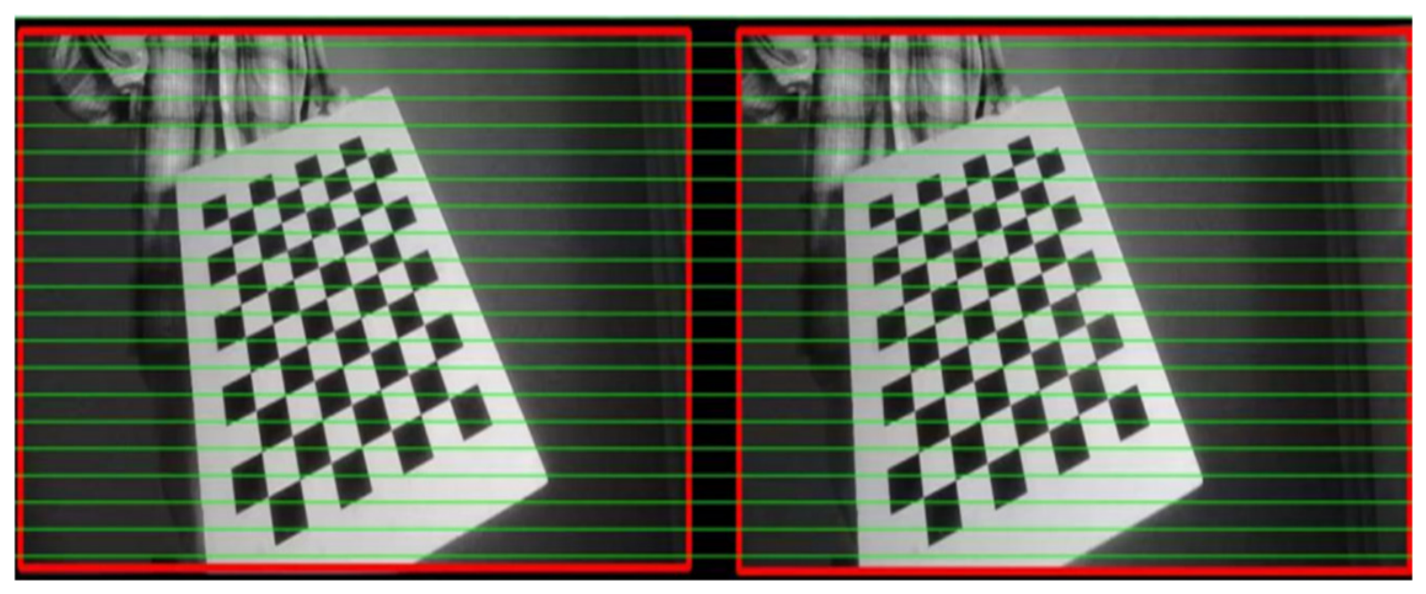
Figure 13 compares the stereo images before and after rectification. After rectification, corresponding image features were aligned more closely along the same pixel rows, reducing vertical disparity and simplifying the subsequent stereo-matching search.

3.2.3. Comparison of Stereo Matching Algorithm

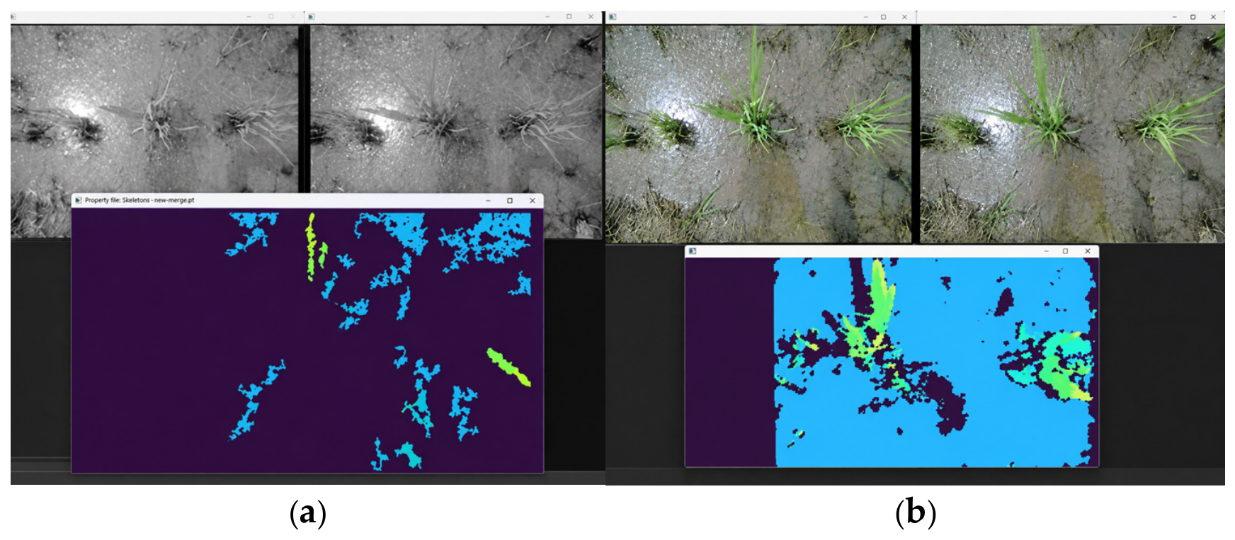
BM and SGBM were compared using stereo images of rice seedlings. Their processing times on a PC were 0.443 s and 0.453 s, respectively. Figure 14 shows example disparity outputs from the two algorithms. Because the input scenes differ, this figure is only used to illustrate the output format and is not intended for direct comparison of matching accuracy or disparity completeness. In this study, SGBM was used to generate disparity maps for the spatial coordinate computation in Section 2.3.4. The above time records are not intended to demonstrate that the system meets the real-time requirements of dynamic field operations.

The SGBM parameters were minDisparity = 0, numDisparities = 96, blockSize = 9, P1 = 8 × channels × blockSize², P2 = 32 × channels × blockSize², disp12MaxDiff = 1, uniquenessRatio = 10, speckleWindowSize = 100, speckleRange = 2, and mode = OpenCV.SGBM.MODE_SGBM_3WAY.

3.2.4. Rice Seedling Localization Accuracy and Error Analysis

The coordinates of rice seedlings before and after camera movement are shown in

Table 8. Rice seedling coordinates before and after camera movement.

Seedling No.	Before Movement/mm	After Movement/mm	X-Axis Displacement/mm	Y-Axis Displacement/mm
1	(12.36, 15.24)	(74.19, −43.22)	61.83	−58.46
2	(85.17, 28.63)	(143.96, −33.34)	58.79	−61.97
3	(−74.28, 69.15)	(−11.67, 10.37)	62.61	−58.78
4	(3.42, 61.38)	(61.44, −0.30)	58.02	−61.68
5	(24.53, −70.44)	(−36.99, −11.87)	−61.52	58.57
6	(132.58, −66.37)	(74.79, −4.51)	−57.79	61.86
7	(68.25, −50.18)	(6.61, 8.37)	−61.64	58.55
8	(149.74, −20.53)	(91.62, 40.97)	−58.12	61.50

Note: The data represent one trial. Disparities used to calculate coordinates were sampled from the SGBM disparity map, not from the horizontal offset between the left and right detection box centers. The statistical results in Table 9 are based on five repeated measurements at each position.

.

The relative localization errors calculated for each test position are presented in

Table 9. Relative localization errors along the X and Y axes.

Seedling No.	X-Axis Error Rate/%	Y-Axis Error Rate/%
1	3.40 ± 1.16	2.87 ± 2.03
2	3.04 ± 1.88	3.28 ± 1.34
3	4.68 ± 2.41	3.20 ± 1.62
4	4.17 ± 1.42	3.73 ± 1.86
5	1.59 ± 0.88	1.74 ± 1.50
6	2.01 ± 1.03	3.13 ± 2.46
7	2.51 ± 1.63	1.42 ± 0.79
8	4.63 ± 3.53	4.80 ± 3.74
Mean error rate	3.25 ± 1.18	3.02 ± 1.07

Note: For each seedling, the error rate is presented as mean ± sample standard deviation (n = 5 repeated measurements). The final row shows the mean ± sample standard deviation across the eight seedling means.

. RMSE was calculated based on all 40 measurements, while the 95% CIs were calculated based on the eight position means (n = 8).

The reported mean relative localization errors were 3.25 ± 1.18% along X and 3.02 ± 1.07% along Y. For a nominal 60 mm translation, these rates correspond to absolute errors of approximately 1.95 and 1.81 mm, respectively.

The RMSE values were 2.31 mm along X and 2.21 mm along Y, respectively. The 95% CIs for the mean error rates were [2.26%, 4.24%] and [2.13%, 3.91%], respectively. The results indicate that the binocular localization system achieved acceptable accuracy in the horizontal plane for coordinate changes in the X and Y directions at a working distance of approximately 650 mm under the experimental conditions of this study.

3.3. Functional Verification of the Seedling-Avoidance- System

To assess functional integration on the terminal device, the trained SE-YOLOv8s model and binocular localization pipeline were deployed on a Raspberry Pi 4B and connected to the prototype seedling-avoidance mechanism.

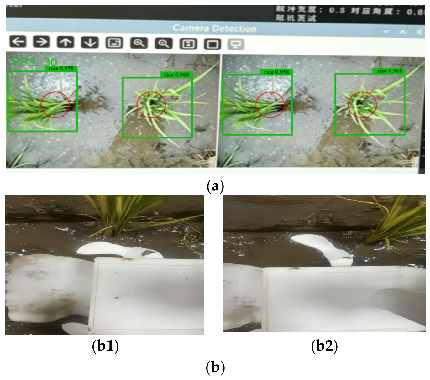
Figure 15a shows representative seedling detection produced on the Raspberry Pi. The system output bounding boxes and class labels that generally covered the seedling canopies. During integrated testing, the Raspberry Pi calculated seedling coordinates from the stereo images and compared the forward distance with the avoidance threshold. Using the 80 mm trigger and 90 mm reset thresholds, the controller output PWM signals that caused the oscillating weed-pressing plate to deflect (Figure 15b). This test confirmed functional communication among the detector, binocular module, controller, and servo actuator.

The prototype completed detection, coordinate reconstruction, and servo actuation on the Raspberry Pi platform, demonstrating functional system integration under the bench-test conditions.

This experiment tested module coordination and mechanical actuation only. Dynamic performance measures, including total system latency, servo response time, avoidance success rate, and seedling damage rate, have yet to be quantified.

4. Discussion

This study developed an SE-YOLOv8s rice seedling model, a binocular localization method, and a Raspberry Pi-based avoidance prototype. Functional integration was demonstrated under bench-top conditions.

At the tillering stage, small rice seedlings, overlapping leaves, and complex backgrounds can cause missed detections and false positives. Inserting SE after SPPF recalibrates channel responses before feature fusion in the neck, potentially increasing the contribution of informative seedling features. The changes in Figure 12 are consistent with this interpretation: compared with YOLOv8s, SE-YOLOv8s produced fewer missed detections and unmatched predictions on the selected images, AP50 also increased in the single-seedling and four-seedling tests, and the position ablation and attention module comparisons favored SE after SPPF on this dataset. Huang et al. [31] and Zhao et al. [32] addressed intra-row single-plant detection and rice planting-condition detection, respectively; although their tasks differ from the task in this study, they face the same balance between detection accuracy and model complexity. Compared with these studies, this work further connects binocular localization and avoidance actuation to detection, making the choice of detection configuration serve subsequent localization and control rather than detection metrics alone.

With a nominal 60 mm translation, the mean errors were approximately 1.95 mm along X and 1.81 mm along Y, consistent with the expected coordinate changes. This consistency is directly relevant to avoidance control, because the controller determines avoidance timing by comparing the seedling position with the reference point across successive frames. The position used for this comparison is the canopy detection box center, which is a visual reference point rather than the stem base. The canopy center may be near the stem base in small seedlings, but leaf expansion and occlusion can increase their separation. Leaf movement, occlusion, water reflections, vibration, and left-right acquisition asynchrony further affect the detection box center or stereo matching. The translation test verified the consistency of differential coordinate changes, whereas absolute distance accuracy also involves calibration error, mounting offset, and canopy-to-stem-base offset. These effects require separate evaluation near the control thresholds. Previous binocular vision studies have mostly addressed crop-row detection or obstacle localization, such as multi-crop-row detection [33] and field obstacle localization [22]. Differences in target size and working distance prevent their localization accuracy estimates from being transferred directly to single-seedling avoidance.

The bench test showed that a command based on estimated seedling coordinates could deflect the weed-pressing plate, demonstrating a functional link between perception and actuation. Whether avoidance can occur in time at operating speeds depends on the combined processing and actuation delay relative to forward speed; this must be assessed in the field. Earlier machine-vision weeding studies have mostly focused on navigation and control, including row guidance integrated with GPS [34] and the visual navigation algorithm for paddy-field robots [35]. This study integrated detection, localization, and actuation in a mechanical weeding device and demonstrated their functional integration under bench-top conditions.

Field performance needs to be evaluated using indicators such as seedling injury rate and weeding rate; for example, Ju et al. [3] reported a weeding rate of 82.4% and a seedling injury rate of 2.8%. In addition, Liu et al. [5] noted that mechanical weeding performance is related to operation timing, whereas Jacquet et al. [36] further showed that the economic feasibility of replacing herbicides with mechanical weeding also depends on yield, cost, and working efficiency. The present perception-actuation system provides a basis for field trials, but its field performance still needs to be confirmed in subsequent field experiments through seedling injury rate, weeding rate, and economic indicators.

Future work is to connect the existing perception method with dynamic field experiments, including end-to-end latency and servo accuracy, absolute forward-distance accuracy near the thresholds, canopy-to-stem-base offset, and seedling injury rate and weeding rate under specified forward speeds and weed conditions. Broader image evaluation and embedded optimization can then be assessed by their contribution to the balance between seedling protection and weed suppression. These efforts will determine the field applicability of the perception–actuation system beyond bench-top validation.

5. Conclusions

This study developed a rice seedling detection and avoidance system for mechanical weeding in paddy fields, integrating SE-YOLOv8s detection, binocular localization, and servo-driven avoidance actuation. The main conclusions are as follows:

(1)

The SE-YOLOv8s configuration improved on the YOLOv8s baseline in both the single-seedling and four-seedling scenarios and obtained the highest values of the reported detection metrics among the tested attention configurations. Because each attention configuration was trained only once, the advantage over ECA-YOLOv8s (0.6–0.7 percentage points in AP50) is reported as a descriptive comparison rather than as a statistically supported difference.

(2)

Binocular localization showed high consistency for coordinate changes at a fixed working distance. The mean errors were approximately 1.95 mm in X and 1.81 mm in Y, providing a usable position reference for avoidance control.

(3)

The bench test demonstrated that the perception output can drive the avoidance actuator, verifying the basic feasibility of the perception-actuation system.

This study provides a technical approach to selective mechanical weeding in paddy fields. However, stem-base localization accuracy, timely avoidance during travel, and field weed suppression have not yet been established, and field application still requires further validation under real operating conditions.

References

1. Bandumula, N. Rice production in Asia: Key to global food security. Proc. Natl. Acad. Sci. India B Biol. Sci. 2018, 88, 1323–1328. [Google Scholar] [CrossRef] [Scilit]
2. Vu, D.H.; Phan, T.T. Rice-Weed Competition Under Different Water Management Systems and Sustainable Weed Control Strategies. Weed Res. 2025, 65, e70034. [Google Scholar] [CrossRef] [Scilit]
3. Ju, J.; Chen, G.; Lv, Z.; Zhao, M.; Sun, L.; Wang, Z.; Wang, J. Design and experiment of an adaptive cruise weeding robot for paddy fields based on improved YOLOv5. Comput. Electron. Agric. 2024, 219, 108824. [Google Scholar] [CrossRef] [Scilit]
4. Dilipkumar, M.; Chuah, T.S.; Goh, S.S.; Sahid, I. Weed management issues, challenges, and opportunities in Malaysia. Crop Prot. 2020, 134, 104347. [Google Scholar] [CrossRef] [Scilit]
5. Liu, C.; Yang, K.Q.; Chen, Y.; Qi, L.; Feng, X.; Tang, Z.Y.; Fu, D.B.; Qi, L. Benefits of mechanical weeding for weed control, rice growth characteristics and yield in paddy fields. Field Crops Res. 2023, 293, 108852. [Google Scholar] [CrossRef] [Scilit]
6. Machleb, J.; Peteinatos, G.G.; Kollenda, B.L.; Andújar, D.; Gerhards, R. Sensor based mechanical weed control: Present state and prospects. Comput. Electron. Agric. 2020, 176, 105638. [Google Scholar] [CrossRef] [Scilit]
7. Slaughter, D.C.; Giles, D.K.; Downey, D. Autonomous robotic weed control systems: A review. Comput. Electron. Agric. 2008, 61, 63–78. [Google Scholar] [CrossRef] [Scilit]
8. Darbyshire, M.; Coutts, S.; Bosilj, P.; Sklar, E.; Parsons, S. Review of weed recognition: A global agriculture perspective. Comput. Electron. Agric. 2024, 227, 109499. [Google Scholar] [CrossRef] [Scilit]
9. Liu, J.; Abbas, I.; Noor, R.S. Development of deep learning-based variable rate agrochemical spraying system for targeted weeds control in strawberry crop. Agronomy 2021, 11, 1480. [Google Scholar] [CrossRef] [Scilit]
10. Quan, L.; Jiang, W.; Li, H.; Li, H.; Wang, Q.; Chen, L. Intelligent intra-row robotic weeding system combining deep learning technology with a targeted weeding mode. Biosyst. Eng. 2022, 216, 13–31. [Google Scholar] [CrossRef] [Scilit]
11. Wang, J.F.; Zhu, P.Y.; Chu, Y.H. Design and experiment of precision spray-type adaptive weeder for paddy fields. Trans. Chin. Soc. Agric. Mach. 2025, 56, 195–205. [Google Scholar]
12. Liao, J.; Chen, M.; Zhang, K.; Zhou, H.; Zou, Y.; Xiong, W.; Zhang, S.; Kuang, F.; Zhu, D. SC-Net: A new strip convolutional network model for rice seedling and weed segmentation in paddy field. Comput. Electron. Agric. 2024, 220, 108862. [Google Scholar] [CrossRef] [Scilit]
13. Upadhyay, A.; Zhang, Y.; Koparan, C.; Rai, N.; Howatt, K.; Bajwa, S.; Sun, X. Advances in ground robotic technologies for site-specific weed management in precision agriculture: A review. Comput. Electron. Agric. 2024, 225, 109363. [Google Scholar] [CrossRef] [Scilit]
14. Deng, X.; Qi, L.; Liu, Z.; Liang, S.; Gong, K.; Qiu, G. Weed target detection at seedling stage in paddy fields based on YOLOX. PLoS ONE 2023, 18, e0294709. [Google Scholar] [CrossRef] [Scilit] [PubMed]
15. Zhang, Q.; Wang, J.H.; Li, B. Extraction method for centerlines of rice seedlings based on YOLOv3 target detection. Trans. Chin. Soc. Agric. Mach. 2020, 51, 34–43. [Google Scholar]
16. Wang, S.S.; Yu, S.S.; Zhang, W.Y. The seedling line extraction of automatic weeding machinery in paddy field. Comput. Electron. Agric. 2023, 205, 107648. [Google Scholar] [CrossRef] [Scilit]
17. Ju, J.; Ma, X.; Yang, C.; Qian, F.; Wang, J.; Chen, G. Lightweight detection method for weeds in complex paddy fields based on the improved YOLOv5. Smart Agric. Technol. 2025, 12, 101418. [Google Scholar] [CrossRef] [Scilit]
18. Yang, X.J.; Zhong, J.B.; Lin, K.Y. Research progress on binocular stereovision technology and its applications in smart agriculture. Trans. Chin. Soc. Agric. Eng. 2025, 41, 27–39. [Google Scholar]
19. Li, Y.; Feng, Q.; Lin, J.; Hu, Z.; Lei, X.; Xiang, Y. 3D locating system for pests’ laser control based on multi-constraint stereo matching. Agriculture 2022, 12, 766. [Google Scholar] [CrossRef] [Scilit]
20. Dadashzadeh, M.; Abbaspour-Gilandeh, Y.; Mesri-Gundoshman, T.; Sabzi, S.; Arribas, J.I. A stereoscopic video computer vision system for weed discrimination in rice field under both natural and controlled light conditions by machine learning. Measurement 2024, 237, 115072. [Google Scholar] [CrossRef] [Scilit]
21. Yang, Y.K.; Liang, C.Q.; Hu, L.; Luo, X.W.; He, J.; Wang, P.; Huang, P.K.; Gao, R.T.; Li, J.H. A proposal for lodging judgment of rice based on binocular camera. Agronomy 2023, 13, 2852. [Google Scholar] [CrossRef] [Scilit]
22. Zhang, Y.Y.; Tian, K.P.; Huang, J.C.; Wang, Z.L.; Zhang, B.; Xie, Q. Field obstacle detection and location method based on binocular vision. Agriculture 2024, 14, 1493. [Google Scholar] [CrossRef] [Scilit]
23. Zhu, F.; Zhang, W.; Zhao, Q.; Meng, X.; Zhao, C.; Feng, W. Improved agricultural machinery navigation algorithm based on machine learning and machine vision technology. Inf. Technol. Control 2025, 54, 396–412. [Google Scholar] [CrossRef] [Scilit]
24. Yang, L.J.; Liu, J.Z.; Tang, X.O. Depth from water reflection. IEEE Trans. Image Process. 2015, 24, 1235–1243. [Google Scholar] [CrossRef] [Scilit] [PubMed]
25. Wang, S.; Yu, S.; Wang, X. An identification algorithm of lateral correction amount for the weeding components in paddy fields based on multi-sensor fusion. Meas. Sci. Technol. 2024, 35, 066301. [Google Scholar] [CrossRef] [Scilit]
26. Zhang, L.F.; Tian, Y. Improved YOLOv8 multi-scale lightweight vehicle object detection algorithm. Comput. Eng. Appl. 2024, 60, 129–137. [Google Scholar]
27. Hu, J.; Shen, L.; Sun, G. Squeeze-and-Excitation Networks. In Proceedings of the IEEE Conference on Computer Vision and Pattern Recognition, Salt Lake City, UT, USA, 18–22 June 2018. [Google Scholar]
28. Zhang, Z. A flexible new technique for camera calibration. IEEE Trans. Pattern Anal. Mach. Intell. 2000, 22, 1330–1334. [Google Scholar] [CrossRef] [Scilit]
29. Bouguet, J.-Y. Camera Calibration Toolbox for MATLAB. Available online: https://www.vision.caltech.edu/bouguetj/calib_doc/ (accessed on 23 September 2026).
30. Hirschmuller, H. Stereo processing by semiglobal matching and mutual information. IEEE Trans. Pattern Anal. Mach. Intell. 2008, 30, 328–341. [Google Scholar] [CrossRef] [Scilit] [PubMed]
31. Huang, S.P.; Wu, S.H.; Sun, C.; Ma, X.; Jiang, Y.; Qi, L. Deep localization model for intra-row crop detection in paddy field. Comput. Electron. Agric. 2020, 169, 105203. [Google Scholar] [CrossRef] [Scilit]
32. Zhao, B.; Zhang, Q.; Liu, Y.; Cui, Y.; Zhou, B. Detection method for rice seedling planting conditions based on image processing and an improved YOLOv8n model. Appl. Sci. 2024, 14, 2575. [Google Scholar] [CrossRef] [Scilit]
33. Zhai, Z.Q.; Zhu, Z.X.; Du, Y.F.; Song, Z.H.; Mao, E.R. Multi-crop-row detection algorithm based on binocular vision. Biosyst. Eng. 2016, 150, 89–103. [Google Scholar] [CrossRef] [Scilit]
34. Kanagasingham, S.; Ekpanyapong, M.; Chaihan, R. Integrating machine vision-based row guidance with GPS and compass-based routing to achieve autonomous navigation for a rice field weeding robot. Precis. Agric. 2020, 21, 831–855. [Google Scholar] [CrossRef] [Scilit]
35. Zhang, Q.; Chen, M.E.S.J.; Li, B. A visual navigation algorithm for paddy field weeding robot based on image understanding. Comput. Electron. Agric. 2017, 143, 66–78. [Google Scholar] [CrossRef] [Scilit]
36. Jacquet, F.; Delame, N.; Vita, J.L.; Huyghe, C.; Reboud, X. The micro-economic impacts of a ban on glyphosate and its replacement with mechanical weeding in French vineyards. Crop Prot. 2021, 150, 105778. [Google Scholar] [CrossRef] [Scilit]
Figure 1. Overall flowchart for the research and development of a seedling-avoidance weeding device for paddy fields.
Applsci 16 09960 g001
Figure 2. Schematic of the paddy field weeding device. 1. Hitch frame; 2. Outer frame; 3. Binocular camera; 4. Limit frame; 5. Parallel four-bar linkage; 6. Inter-row grass-pressing plate; 7. Mud guide plate; 8. Bionic intra-row weeding shovel.
Applsci 16 09960 g002
Figure 3. Representative data-processing results: (a) Original image; (b) Gaussian blur; (c) Gaussian noise; (d) Gamma correction; (e) Increased brightness.
Applsci 16 09960 g003
Figure 4. Architecture of SE-YOLOv8s.
Applsci 16 09960 g004
Figure 5. Architecture of the squeeze-and-excitation module.
Applsci 16 09960 g005
Figure 6. Checkerboard for calibration.
Applsci 16 09960 g006
Figure 7. Relationships among the four coordinate systems.
Applsci 16 09960 g007
Figure 8. Test platform for evaluating binocular localization accuracy. 1. Rice Seedlings; 2. X-Axis of the Test Bench; 3. Binocular Recognition Camera; 4. Test Bench Operation Terminal; 5. Y-Axis of the Test Bench; 6. Motor Power Supply of the Test Bench; 7. Test Bench Controller.
Applsci 16 09960 g008
Figure 9. Simplified hardware-connection diagram for the seedling-avoidance system. 1. External Power Supply; 2. Voltage Regulator Module; 3. Servo Motor 1; 4. Raspberry Pi; 5. Servo Motor 2; 6. Binocular Camera.
Applsci 16 09960 g009
Figure 10. Control workflow of the seedling-avoidance system.
Applsci 16 09960 g010
Figure 11. Training and validation loss curves of YOLOv8s and SE-YOLOv8s.
Applsci 16 09960 g011
Figure 12. Detection results comparison between YOLOv8s and SE-YOLOv8s for rice seedlings.
Applsci 16 09960 g012
Figure 13. Binocular images before and after rectification.
Applsci 16 09960 g013
Figure 14. Disparity output examples: (a) BM; (b) SGBM.
Applsci 16 09960 g014
Figure 15. Functional verification of the integrated seedling-avoidance system. (a) Rice seedling detection on Raspberry Pi terminal, (b) Oscillating weed-pressing plate deflection test, (b1) Before deflection, (b2) After deflection.
Applsci 16 09960 g015