Predicting Avian Observation Patterns in Mediterranean Wetlands: Spatiotemporal Deep Learning Fusion of Multi-Source Surveys, Citizen Science, and Autonomous Acoustic Sensing

Abstract

Protected wetlands in the Mediterranean are vital biodiversity hotspots that face growing pressure from climate change and human activity. Traditional bird monitoring relies on professional field surveys, which, although highly standardized, are resource-constrained and limited in temporal frequency. Here, we present ValWet-Birds, a multi-source spatiotemporal dataset and fusion framework that harmonises and integrates professional counts, eBird citizen science registries, and passive acoustic monitoring (via a BirdNET classifier deployed on a Raspberry Pi 5 node) for three protected wetlands in Alicante, Spain (El Hondo, Santa Pola, and La Mata–Torrevieja), from 2010 to 2025. We normalize incompatible observation protocols into a unified monthly relative observation proportion target across 12 sub-regions and 394 taxa (349 resolved to species level after a taxonomic audit). Spatiotemporal prediction models are implemented using Multi-Layer Perceptron (MLP) and Long Short-Term Memory (LSTM) neural networks. A preliminary evaluation using non-matched test sets suggested a 42.7% reduction in Test Mean Squared Error for the LSTM under multi-source augmentation. Re-evaluating every source condition on an identical held-out set of professional-census observations shows that this benefit does not hold in aggregate: both baselines outperform naive temporal reference predictors by a wide margin, but adding eBird and BirdNET data does not reduce error relative to census-only training overall. The exception is conservation-relevant taxa (a 50-species subset cross-referenced against Annex I of the EU Birds Directive), for which multi-source augmentation reduces LSTM error by 29% and MLP error by 9%, plausibly because these less-common species have sparser census history to draw on. We report this reversal explicitly as a methodological finding in its own right. Finally, we describe the design and interactive user flows of the deployed web visualization platform Avistory, which presents observation summaries and model outputs; it should not be interpreted as a validated population-monitoring or conservation-decision system.

1. Introduction

Global biodiversity is facing unprecedented challenges due to anthropogenic pressures, habitat fragmentation, and climate change [1]. Wetlands are among the most biodiverse and ecologically sensitive ecosystems on Earth, playing a vital role in supporting waterbird populations [2]. Birds, in particular, serve as excellent ecological indicators for monitoring ecosystem health due to their sensitivity to environmental alterations, wide distribution, and relative ease of observation compared to other taxa [3]. In the Mediterranean region, protected wetlands are critical stopover points for migratory routes and breeding grounds for numerous threatened species. Specifically, the wetlands in the southern Valencian Community of Spain (Parc Natural d’El Hondo, Salinas de Santa Pola, and Lagunas de La Mata–Torrevieja) represent critical habitats designated as Important Bird Areas (IBAs) and protected under the Ramsar Convention [4,5].

However, monitoring avian populations in these ecosystems is historically challenging. Traditional monitoring relies on professional field censuses conducted by ornithologists [6,7]. While these surveys are highly standardized and provide reliable population counts, they are resource-intensive, expensive, and limited in spatiotemporal resolution, often conducted only once a month or seasonally. This sparsity can fail to capture rapid shifts in bird distribution or migration timings.

To supplement traditional surveys, two main paradigms have emerged: citizen science and autonomous monitoring. Citizen science platforms, most notably eBird [8,9], have revolutionized ecological research by aggregating millions of bird sightings submitted by recreational birdwatchers worldwide. These platforms offer unprecedented spatial and temporal coverage [10]. Nevertheless, citizen science data suffer from significant limitations, including spatial and temporal clustering, varying observer expertise, and a lack of standardized effort (e.g., presence-only checklists) [11]. These limitations are part of a broader, well-documented literature on bias and information content in biological records [12] and on the consequences of imperfect and heterogeneous detection for species distribution and occupancy modeling [13,14], which motivates treating our target as an observation-process outcome rather than as a direct estimate of occurrence or detection probability. Conversely, autonomous monitoring technologies, such as Internet of Things (IoT) acoustic sensors deployed in the wild running deep-learning classifiers like BirdNET [15], offer continuous, non-intrusive, and high-frequency recording of bird vocalizations [16]. Yet, these sensors are localized to single points, produce large volumes of detections that do not correspond directly to abundance, and are vulnerable to physical hazards (such as sensor failures due to seasonal flooding in wetland environments). These sources therefore represent different observation processes: a census count records individuals during a standardized survey, an eBird record depends on observer effort and reporting, and a BirdNET detection records an acoustic classifier output that may include repeated vocalizations from one individual. Their numerical harmonisation does not make them biologically equivalent.

To address these limitations, researchers must combine these heterogeneous data sources to generate robust spatiotemporal occurrence models [17]. Fusing citizen science, acoustic sensor networks, and professional censuses requires overcoming major differences in count methodologies, spatial resolution, and temporal coverage. In particular, professional censuses record absolute counts, eBird checklists register mixed presence-only and count data, and acoustic sensors record detection counts of vocalizations. Fusing them at the count level is impossible; thus, a standardized representation is required.

In this work, we present a comprehensive framework for multi-source bird observation modeling and interactive visualization in Valencian wetlands. Our working hypothesis is that adding denser but heterogeneous observations can improve prediction of the held-out observation proportions by supplying temporal and spatial context, while not necessarily correcting source-specific sampling or detection bias. The framework is therefore a predictive baseline rather than an occupancy model or a direct estimator of population status. The key contributions of this paper are as follows:

• ValWet-Birds Dataset: We construct and release a harmonized multi-source spatiotemporal dataset that taxonomically and spatially unifies citizen science (eBird), autonomous acoustics (BirdNET from Raspberry Pi devices), and professional censuses across three protected wetlands, resolving them into a single, cohesive resource spanning from 2010 to 2025 across 12 sub-regions and 394 taxa (349 resolved to species level, Section 2.4).
• Spatiotemporal Deep Learning Baseline: We present and evaluate two baseline deep learning architectures, a Feed-Forward MLP and an LSTM recurrent network, trained to predict the relative observation proportion of bird species.
• Rigorous Data Augmentation Evaluation: We first report a preliminary comparison (differently sized test sets) showing a 42.7% MSE reduction under augmentation, and then re-evaluate every source condition on an identical held-out set of professional-census observations. The aggregate benefit does not survive this stricter comparison, but a 50-taxon subset cross-referenced against Annex I of the EU Birds Directive does show a substantial, consistent benefit from augmentation (29% MSE reduction for the LSTM). We report both results and the reversal between them as a methodological contribution.
• Interactive Web Visualizer: We have created Avistory, an open-source, interactive web visualization system that enables researchers and the public to intuitively query, filter, and visualize historical observations alongside our deep learning model predictions.

The remainder of this paper is structured as follows. Section 2 presents the study area, data sources, harmonisation pipeline, and relative observation proportion normalization. Section 3 outlines the MLP and LSTM baseline models, sequence generation, and training protocol. Section 4 reports the model performance and the quantitative benefits of data augmentation. Section 5 describes the design and user flows of the Avistory visualization platform. Finally, Section 6 and Section 7 discuss the limitations, future lines of research, and conclusions.

2. Materials and Methods

2.1. Study Area

The study area encompasses three protected wetlands located in the province of Alicante, within the Valencian Community in southeastern Spain. These areas are designated as Important Bird Areas (IBAs) and are characterized by diverse hydrological and ecological regimes:

• Parque Natural El Hondo (IBA BIRDLIFE_1824): Composed of multiple reservoirs and marshlands. It contains both freshwater reservoirs (e.g., Embalse de Levante and Embalse de Poniente) and saline lagoons, supporting a rich biodiversity of waterfowl.
• Salinas de Santa Pola (IBA BIRDLIFE_1825): A coastal saltpan wetland characterized by high salinity, including active salt-extraction basins and littoral zones.
• Lagunas de La Mata y Torrevieja (IBA BIRDLIFE_1826): Composed of two large hypersaline lagoons. The Laguna de Torrevieja is highly hypersaline, supporting minimal avian life (mostly restricted to nesting areas on salt dikes), while the Laguna de La Mata is slightly less saline, supporting larger populations of flamingos and grebes.

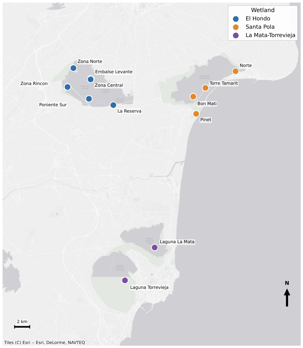
To conduct fine-grained spatiotemporal modeling, these three wetlands were partitioned into 12 survey units (sub-regions), corresponding to specific water bodies or management sectors (

Table 1. Wetlands and their corresponding 12 sub-regions.

Wetland	IBA Code	Sub-Regions
Parc Natural d’El Hondo	BIRDLIFE_1824	Embalse Levante, Zona Central, Poniente Sur, La Reserva, Zona Rincón, Zona Norte
Salinas de Santa Pola	BIRDLIFE_1825	Pinet, Torre Tamarit, Bon Matí, Norte
Lagunas de La Mata–Torrevieja	BIRDLIFE_1826	Laguna La Mata, Laguna Torrevieja

, Figure 1).

2.2. Data Sources

The dataset is constructed by harmonising and integrating three independent, heterogeneous observation sources:

• Citizen Science: Observation records retrieved from the eBird Dataset (ES-VC regional release, November 2025) [8]. Sightings were filtered spatially using bounding boxes matching the three target IBA codes, covering the period from January 2010 to December 2025.
• Professional Census: Standardized monthly bird counts conducted by professional ornithologists using exhaustive visual and auditory counts, following a protocol comparable in spirit to the International Waterbird Census [18] but conducted monthly rather than as a single coordinated mid-winter count. It covers the year 2025 for all three wetlands, and 2024 for Santa Pola. Only the 2024–2025 records were digitized and shared with us by the regional management authority in a format compatible with this dataset; an extended historical archive, if one exists, was not accessible to us for this study, and we do not assume otherwise. Survey duration, the number of observers per count, exact survey timing, and the procedures used to avoid double-counting were likewise not provided to us and are not reconstructed here; we report their absence as a limitation of the available metadata rather than an assumption about the census protocol. Water level, salinity, weather, observer effort, checklist duration, and completeness were not available to us as measured covariates for any of the three sources and are not included in the models presented here. These surveys provide high-quality absolute abundance data but are limited to monthly intervals.
• Autonomous Acoustics: Passive acoustic monitoring data were collected by an IoT sensor node based on a Raspberry Pi 5 (Raspberry Pi Ltd., Cambridge, UK) deployed at El Hondo. The sensor continuously recorded ambient audio and identified bird vocalizations from 24 September 2024 to 10 May 2025 using the pre-trained BirdNET convolutional neural network classifier [15]. Detections were filtered to keep only those with a confidence score $\ge 0.7$.

The resulting ValWet-Birds dataset contains 67,787 observation rows, covering 190 unique year-months (from January 2010 to December 2025) across 394 taxa (

Table 2. Observation counts and distribution across the three sources.

Source	Description	Observations
eBird	Citizen science checklists	62,824
Census	Professional surveys	4626
BirdNET	Raspberry Pi 5 audio sensor	337
Total	Combined dataset	67,787

; see Section 2.4 for the taxonomic audit that resolved this count from an initial 395).

2.3. Spatial Harmonisation

Integrating these sources required resolving differing spatial identifiers. Professional censuses record observations at the level of local micro-zones and management units (e.g., Eb.Levante, CALENTADORES, Punta Víbora). eBird records contain user-defined text descriptions of hotspots (e.g., El Hondo PNat–Embalse de Levante) or arbitrary coordinates for personal checklists. BirdNET files do not record specific sub-regions on the device.

Spatial harmonisation was completed in two steps:

• Keyword and Lookup Mapping: A manually curated mapping table was built to associate known eBird hotspots and professional census micro-zones directly with the corresponding 12 unified sub-regions. For the BirdNET sensor, since it was statically placed, all records were mapped to the El Hondo–La Reserva sub-region.
• Nearest-Centroid Fallback: eBird checklists not associated with a predefined hotspot instead carried individual GPS coordinates. For these records, we calculated the geographic distance (Haversine) to the centroids of all 12 sub-regions. If a coordinate fell within a 500-m buffer of the nearest centroid, it was automatically assigned to that sub-region; checklists beyond this buffer from every centroid were excluded.

The resulting 12 sub-regions are treated as survey units selected to balance geographical granularity with observation density, ensuring that every unit has either significant census coverage or ≥800 eBird checklist entries. They should not be interpreted as homogeneous ecological units, because habitat composition, water depth, salinity, and vegetation may vary within and among them.

Spatial-assignment counts. We reconstructed this procedure over the 13,975 eBird checklists falling within the three target IBAs, using the same keyword-mapping table and 500 m centroid buffer described above: 10,684 checklists (76.5%) matched a known hotspot directly (Step 1); of the remaining 3291 checklists carrying individual coordinates, 2192 (15.7% of the total; 66.6% of the coordinate-only subset) were assigned via the nearest-centroid fallback (Step 2), and 1099 (7.9% of the total; 33.4% of the coordinate-only subset) fell outside the 500 m buffer of every centroid and were excluded. In total, 12,876 checklists (92.1%) were retained. The reconstruction reported here was run directly against the archived eBird sampling file using a mapping table and buffer threshold.

2.4. Taxonomic Harmonisation

Avian nomenclature varies across sources. The professional census uses local scientific names directly. eBird records provide scientific and common Spanish/English names. BirdNET outputs English common names with underscores (e.g., Barn_Swallow, Cettis_Warbler), which occasionally conflict with eBird naming conventions.

To address discrepancies in species naming across data sources, all recorded taxa were standardized to their corresponding scientific names. This harmonization step unified the nomenclature across sensor detections, citizen science records, and professional surveys, yielding a consolidated vocabulary of 394 taxa (349 resolved to species level), following the taxonomic audit described below.

Taxonomic audit. We audited every distinct scientific-name label in the dataset. This identified one clear nomenclature error: 177 census records (24 year-months, including 31 inside the common evaluation window in Section 4) were labelled Phoenicopterus ruber (American Flamingo), a species absent from this region. Our eBird-derived taxonomy lookup table already lists Phoenicopterus roseus (Greater Flamingo) as the correct name for this taxon, so we treat the Census label as a legacy synonym error and merge these records into Phoenicopterus roseus, matching the label already used by eBird and BirdNET. The audit also found 45 taxa (796 eBird rows, 1.2% of the dataset) recorded only to genus or family level or as slash-notation pairs (e.g., Sturnus vulgaris/unicolor, Anatidae sp.), consistent with eBird’s own conventions for uncertain field identifications; none originate from Census, so they do not affect the common test set. We do not reassign these to a single candidate species, since that would imply an identification the observer did not make; instead, we exclude them from species-level ranking (as detailed in Section 2.6) while retaining them in the dataset and in the denominator of Equation (1). The corrected vocabulary contains 394 scientific-name labels: 349 resolved species and 45 unresolved.

Legal-nomenclature synonyms. Directive 2009/147/EC retains the 1979-era scientific names of its predecessor (79/409/EEC), several of which have since been superseded by modern (IOC/Clements) nomenclature. Seven taxa in our Annex I cross-reference (

Table 3. Taxa in our Annex I cross-reference where the modern scientific name (used in this dataset) differs from the 1979 nomenclature name printed in the legal text of Directive 2009/147/EC.

Name in This Dataset	Name in Directive 2009/147/EC	Common Name
Calidris pugnax	Philomachus pugnax	Ruff
Curruca undata	Sylvia undata	Dartford Warbler
Gelochelidon nilotica	Sterna nilotica	Gull-billed Tern
Hydroprogne caspia	Sterna caspia	Caspian Tern
Phoenicopterus roseus	Phoenicopterus ruber (subsp. roseus)	Greater Flamingo
Sternula albifrons	Sterna albifrons	Little Tern
Thalasseus sandvicensis	Sterna sandvicensis	Sandwich Tern

) are listed under such a superseded name in the directive text; all seven are the same taxon under current avian systematics, unrelated to the Phoenicopterus ruber/roseus correction above.

2.5. Unified Relative Probability Target

Fusing abundance data directly from these sources is impossible because their recording protocols are incompatible. eBird checklists represent varying search durations and observer counts, censuses represent absolute visual counts, and BirdNET represents the frequency of vocal detections.

To address this issue, we normalized counts into a relative monthly observation proportion (P) within each grouping of source (s), sub-region (r), year (y), and month (m):

$$P_{s,r,y,m,sp}={\displaystyle \frac{C_{s,r,y,m,sp}}{{\sum }_{s{p}^{\prime }\in \mathcal{S}}{C}_{s,r,y,m,s{p}^{\prime }}}}\times 100$$

(1)

where $C_{s,r,y,m,sp}$ is the count of species $sp$ within the grouping, and $\mathcal{S}$ is the set of all species recorded in that grouping. By construction, ${\sum }_{sp}{P}_{s,r,y,m,sp}=100\%$ for each group.

This formulation allows joint modeling of citizen science, sensors, and professional censuses without mixing incompatible raw units. The resulting value is a source-conditional proportion of recorded detections or counts, not a formal occurrence or detection probability: it depends on the focal species and on all other taxa recorded in the same grouping. Source-specific observation and detection processes are not explicitly modeled, so values from different sources are comparable only as inputs to this predictive baseline and not as equivalent biological measurements. The resulting distribution is right-skewed, reflecting the dominance of a small number of taxa in the recorded data, resulting in a median observation proportion of 0.4% and a 99th percentile of 39.6%.

2.6. Dataset Balance

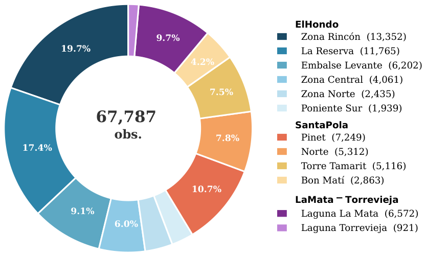
Throughout this subsection, “records” or “observations” refers to rows of the harmonised dataset, i.e., distinct species × sub-region × year × month × source combinations after aggregation (Section 2.5), not to individual raw eBird checklists or field observations submitted before harmonisation. Figure 2 shows how observations are distributed across the 12 sub-regions. El Hondo concentrates 58% of all records, driven mainly by Zona Rincón (19.7%) and La Reserva (17.4%), which are the most accessible areas and the most frequently visited eBird hotspots. Santa Pola accounts for 30% of the dataset, while La Mata–Torrevieja contributes the remaining 11%. The smallest sub-region, Laguna Torrevieja, holds only 921 harmonised records (1.4%; 697 from eBird and 224 from Census), consistent with its hypersaline conditions and limited avian activity.

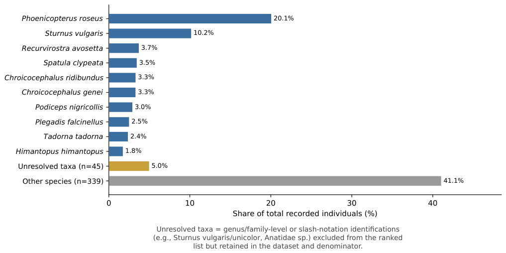
Figure 3 illustrates species concentration by total number of individuals recorded, after the taxonomic audit described above. The top 10 resolved species account for 53.9% of all individuals across the dataset. The Greater Flamingo (Phoenicopterus roseus) alone represents 20.1%, with just over 1,039,000 individuals once the corrected census records are included, followed by Common Starling (Sturnus vulgaris) at 10.2%. A further 5.0% of individuals belong to the 45 genus/family-level or slash-notation taxa that are not assigned to a single resolved species and are therefore excluded from the ranked list. The remaining 339 species share 41.1% of the total count. This heavy concentration is characteristic of wetland avifaunal communities and directly motivates the use of the relative observation proportion normalization described above.

3. Baseline Deep Learning Models

We implement and compare two spatiotemporal neural network baseline models to predict monthly relative observation proportions: a Feed-Forward Multi-Layer Perceptron (MLP) and a recurrent Long Short-Term Memory (LSTM) network. Both models adopt a single-instance formulation where each input instance corresponds to a single $\langle \mathrm{species},\mathrm{sub-region},\mathrm{month},\mathrm{year}\rangle$ tuple and yields a scalar prediction. Consequently, spatial predictions across the entire wetland area are generated by executing 12 independent inference passes (one per sub-region) for any target species and timestep.

Table 4. Notation used in the MLP and LSTM baseline formulations.

Symbol	Definition
$s{p}_{id},s{r}_{id}$	Categorical identifiers for species and sub-region.
$E_{\mathrm{species}}\in {\mathbb{R}}^{N_{\mathrm{species}}\times 64}$	Learned species embedding table, $N_{\mathrm{species}}=395$ (one slot per taxon identifier assigned before the taxonomic audit in Section 2.4; identifiers were not renumbered after the audit merged one taxon, so the table keeps one unused row and the dataset itself has 394 taxa).
$E_{\mathrm{subregion}}\in {\mathbb{R}}^{12\times 8}$	Learned sub-region embedding table.
$m_{\sin },m_{\cos }$	Cyclic sine/cosine encoding of calendar month $m\in [1,12]$.
$y_{\mathrm{scaled}}$	Standardized calendar year (zero mean, unit variance on the training set).
$P_{s,r,y,m,sp}$	Relative observation proportion target (Equation (1)), 0–$100\%$ scale.
T	LSTM sequence length (temporal window), in months.
${\mathbf{f}}_t\in {\mathbb{R}}^4$	LSTM input feature vector at timestep t.
${\mathbf{c}}_{\mathrm{static}}\in {\mathbb{R}}^{72}$	Concatenated species/sub-region embedding used to initialize LSTM state.
${\mathbf{h}}_0,{\mathbf{c}}_0$	Initial LSTM hidden and cell states.
${\mathbf{h}}_T\in {\mathbb{R}}^{64}$	Final LSTM hidden state after processing the input sequence.
${\widehat{P}}_{\mathrm{MLP}},{\widehat{P}}_{\mathrm{LSTM}}$	Model-predicted relative observation proportion.

summarizes the notation used throughout this section to support the mathematical description of the two architectures.

3.1. Feature Representation and Embeddings

To enable effective deep learning, input features are represented using a combination of categorical embeddings and continuous feature normalization:

• Categorical Embeddings: Species IDs are mapped to a 64-dimensional continuous space using an embedding layer ($E_{\mathrm{species}}\in {\mathbb{R}}^{N_{\mathrm{species}}\times 64}$). Sub-region IDs (representing the 12 spatial sectors) are mapped to an 8-dimensional space ($E_{\mathrm{subregion}}\in {\mathbb{R}}^{12\times 8}$). These learned embeddings allow the models to represent taxonomic similarity and spatial correlations.
• Cyclic Temporal Encoding: Calendar months ($m\in [1,12]$) are converted into cyclic 2D coordinate representations to preserve proximity between December and January:

  $$m_{\sin }=\sin \left({\displaystyle \frac{2\pi m}{12}}\right),m_{\cos }=\cos \left({\displaystyle \frac{2\pi m}{12}}\right)$$

  (2)
• Year Normalization: Calendar years are normalized using a standard scaling transformation based on the training set distribution to ensure stability:

  $$y_{\mathrm{scaled}}={\displaystyle \frac{\mathrm{year}-{\mu }_{\mathrm{year}}}{{\sigma }_{\mathrm{year}}}}$$

  (3)

3.2. Multi-Layer Perceptron Architecture

The MLP baseline operates as a static regressor, modeling occurrences for a given species and sub-region at a specific time step independently. The input vector ${\mathbf{x}}_{\mathrm{MLP}}\in {\mathbb{R}}^{75}$ concatenates the continuous features and categorical embeddings:

$$\mathbf{x}\mathrm{MLP}=\left[E_{\mathrm{species}}\left({\mathrm{sp}}_{id}\right)\parallel E_{\mathrm{subregion}}\left({\mathrm{sr}}_{id}\right)\parallel m_{\sin }\parallel m_{\cos }\parallel y_{\mathrm{scaled}}\right]$$

(4)

The model consists of three fully connected hidden layers with dimensions 256, 128, and 64, respectively. To ensure stability during training and prevent overfitting, each linear transformation is sequentially followed by Batch Normalization, a Rectified Linear Unit (ReLU) activation, and Dropout (with a rate of $0.3$). The final scalar output ${\widehat{P}}_{\mathrm{MLP}}$, representing the predicted relative observation proportion percentage, is computed as:

$${\widehat{P}}_{\mathrm{MLP}}={\mathbf{w}}_o^T{\mathbf{h}}_3+b_o$$

(5)

where ${\mathbf{h}}_3\in {\mathbb{R}}^{64}$ is the representation extracted by the last hidden layer, and $\{{\mathbf{w}}_o,b_o\}$ are the parameters of the output layer.

3.3. Long Short-Term Memory Architecture

The LSTM baseline is formulated to capture sequential temporal patterns. For each (sub-region, species) pair, the model processes a sequence of historical observations to predict the relative observation proportion in the subsequent month.

A continuous monthly timeline is built for each species and sub-region. Missing months are zero-filled with their corresponding cyclic temporal features. Sliding windows of sequence length $T=3$ months are constructed. Each timestep $t\in [1,T]$ is represented by a 4D feature vector:

$${\mathbf{f}}_t=\left[m_{\sin }^t,m_{\cos }^t,y_{\mathrm{scaled}}^t,P_t\right]$$

(6)

where $P_t$ is the historical relative observation proportion at month t.

Static metadata is incorporated by concatenating the learned species and sub-region embeddings into a context vector ${\mathbf{c}}_{\mathrm{static}}=\left[E_{\mathrm{species}}\left({\mathrm{sp}}_{id}\right)\parallel E_{\mathrm{subregion}}\left({\mathrm{sr}}_{id}\right)\right]\in {\mathbb{R}}^{72}$. This vector is linearly projected to initialize the initial hidden state ${\mathbf{h}}_0={\mathbf{W}}_p{\mathbf{c}}_{\mathrm{static}}+{\mathbf{b}}_p$, while the cell state ${\mathbf{c}}_0$ is initialized to zero.

The temporal sequence ${\mathbf{f}}_{1:T}$ is processed through a single-layer LSTM with 64 hidden units and recurrent dropout (rate $0.35$). Finally, the last hidden state ${\mathbf{h}}_T\in {\mathbb{R}}^{64}$ is concatenated with the static context ${\mathbf{c}}_{\mathrm{static}}$ and passed through a dense layer with ReLU activation and Dropout ($0.3$) to yield the output prediction:

$${\widehat{P}}_{\mathrm{LSTM}}={\mathbf{w}}_f^T·\mathrm{Dropout}\left(\mathrm{ReLU}\left({\mathbf{W}}_h\left[{\mathbf{h}}_T\parallel {\mathbf{c}}_{\mathrm{static}}\right]+{\mathbf{b}}_h\right)\right)+b_f$$

(7)

where ${\widehat{P}}_{\mathrm{LSTM}}$ denotes the predicted relative observation proportion for month $T+1$.

3.4. Training Protocol and Implementation Details

Both architectures are implemented in PyTorch (version 2.2.0) and trained on a single NVIDIA GeForce RTX 4090 GPU. Models are optimized to minimize the Mean Squared Error (MSE) directly on the target relative observation proportion percentage scale (0–100%).

Optimization is performed using the Adam optimizer with an initial learning rate of ${10}^{-3}$, an $L_2$ weight decay penalty of ${10}^{-5}$, and a batch size of 256 for the MLP and 128 for the LSTM. To facilitate stable convergence, a Cosine Annealing learning rate scheduler dynamically decays the learning rate over a maximum budget of 200 epochs. To mitigate overfitting, early stopping is enforced by monitoring validation loss, terminating training if no improvement is observed for 20 consecutive epochs.

4. Results

4.1. Preliminary Comparison and Its Limitation

To evaluate predictive performance and quantify the impact of multi-source data fusion, models were evaluated chronologically. The final three months of the dataset were held out as the evaluation test set, while all preceding records were used for training.

Evaluations were conducted across two training regimes: (i) Census Only, representing the traditional sparse scenario trained strictly on professional surveys (3807 training and 819 test observations), and (ii) All Sources (Augmented), utilizing the unified dataset combining citizen science (eBird), passive acoustic monitoring (BirdNET), and professional censuses (65,802 training and 1985 test observations). Predictive performance was evaluated using Mean Squared Error (MSE) and Root Mean Squared Error (RMSE) on the target relative observation proportion percentage scale (0–100%). Because the two conditions have different test-set sizes and compositions, the preliminary comparison reported in

Table 5. Preliminary non-matched-test comparison across training conditions (kept for transparency; superseded by the common test-set evaluation described below). Bold values indicate the best performance for each metric.

Model	Training Condition	MSE	RMSE	MAE	${\mathit{R}}^2$	Acc ± 5pp (%)
MLP	Census Only	56.54	7.52	3.66	0.47	79.12
	All Sources (Augmented)	39.02	6.25	2.26	0.43	89.62
LSTM	Census Only	56.08	7.49	3.42	0.42	83.56
	All Sources (Augmented)	32.10	5.67	1.77	0.42	92.32

is descriptive, not a causal estimate of the benefit of augmentation.

The preliminary comparison shows lower error in the augmented condition than in the census-only condition, with the LSTM’s test MSE dropping from 56.08 to 32.10 (a 42.7% reduction). As Section 4.2 shows, this pattern reverses once both conditions are evaluated on identical test rows: part of this apparent gain is an artifact of the All Sources test set containing 1985 rows (dominated by eBird and BirdNET rows with many near-zero targets) rather than the 819 professional-census rows used for Census Only. We retain this table for transparency about what was originally reported; conclusions about the benefit of data augmentation should be drawn from

Table 6. Common test-set comparison: every condition is evaluated on the same 819 held-out professional-census rows (786–812 for LSTM, depending on how many rows have a real 3-month preceding sequence). Neural results are mean ± SD over 3 seeds. Bold values indicate the best performance for each model and metric across training conditions.

Model	Condition	MSE	MAE	${\mathit{R}}^2$	Acc ± 5pp (%)
Persistence (naive)	Census Only	109.49	4.15	−0.03	82.5
Seasonal-naive	Census Only	95.88	3.87	0.09	83.3
MLP	Census Only	57.08 ± 2.36	3.51 ± 0.03	0.461 ± 0.022	81.6 ± 1.0
	Census + eBird	64.82 ± 2.13	3.43 ± 0.03	0.388 ± 0.020	83.4 ± 0.3
	Census + BirdNET	60.06 ± 2.30	3.57 ± 0.11	0.433 ± 0.022	80.5 ± 1.4
	All Sources	66.79 ± 0.86	3.46 ± 0.06	0.369 ± 0.008	83.8 ± 0.6
LSTM ($T=3$)	Census Only	63.28 ± 2.06	3.69 ± 0.08	0.416 ± 0.019	81.6 ± 0.3
	Census + eBird	69.57 ± 2.57	3.30 ± 0.03	0.348 ± 0.024	85.8 ± 0.5
	Census + BirdNET	62.93 ± 0.19	3.73 ± 0.13	0.418 ± 0.002	81.7 ± 1.2
	All Sources	66.73 ± 2.18	3.24 ± 0.03	0.374 ± 0.020	85.8 ± 0.9

, not from this table.

4.2. Common Test-Set Evaluation Across Source Conditions

To address this directly, we re-evaluated every training condition on exactly the same held-out professional-census rows: the last three available year-months (from October 2025 to December 2025, 819 Census rows), with the preceding month (September 2025) held out as a validation period excluded from both training and the final test. We compare four source conditions—Census Only, Census + eBird, Census + BirdNET, and All Sources—against two non-neural reference baselines, persistence (previous calendar month) and seasonal-naive (same calendar month, previous year). The published architectures do not take source identity as an input, so when multiple sources are combined, rows are collapsed to one target per species/sub-region/month by averaging their source-conditional proportions before fitting; this averaging is an explicit, disclosed choice, not an attempt to infer source identity implicitly. Each neural configuration was trained with 3 random seeds (42, 43, 44); we report the mean ± standard deviation across seeds. Table 6 reports the results.

Three findings follow from Table 6. First, both neural architectures clearly outperform the two non-neural reference baselines in MSE (57–67 vs. 96–109), establishing that the deep-learning baselines add value beyond a naive predictor. Second, and contrary to the preliminary comparison in Table 5, adding eBird—and therefore the All Sources condition, which includes eBird—does not reduce MSE relative to Census Only for either architecture; it increases it by 14–17% for the MLP and 5–12% for the LSTM. Adding BirdNET alone has a small, direction-inconsistent effect (a slight increase for the MLP, a marginal decrease for the LSTM) that is within one seed standard deviation of the Census Only result for the LSTM. We therefore do not find evidence, in this common-test comparison, that multi-source augmentation reduces prediction error on the professional-census test rows overall; Section 4.5 shows this is not the whole story once conservation-relevant taxa are considered separately. Third, accuracy at ±5pp is a poor discriminator here: it varies by only 2–5 points across configurations that differ in MSE by up to 17%, which is why we report $R^2$ and MSE as the primary comparison metrics and ±5pp only as a supplementary, coarse indicator (see also the threshold analysis below).

We revise the manuscript’s headline claim accordingly: the 42.7% figure describes a preliminary, non-matched-test comparison and should not be read as evidence that multi-source augmentation improves prediction of professional-census observations in general. What Table 6 does support is that the MLP and LSTM baselines predict the harmonised observation metric substantially better than naive temporal reference points, and that source identity currently matters more for training composition (which rows dilute the signal) than as a source of consistent improvement.

Table 6 reports accuracy at the ±5pp threshold used elsewhere in the manuscript.

Table 7. Threshold accuracy on the common test set: percentage of predictions within 1, 2, and 5 percentage points of the true value.

Model	Condition	Acc ± 1pp (%)	Acc ± 2pp (%)	Acc ± 5pp (%)
Persistence (naive)	Census Only	56.7	66.9	82.5
	Census + eBird	55.6	66.2	82.8
	Census + BirdNET	56.7	66.9	82.5
	All Sources	55.6	66.2	82.8
Seasonal-naive	Census Only	57.5	69.0	83.3
	Census + eBird	56.3	68.0	82.7
	Census + BirdNET	57.4	68.9	83.2
	All Sources	56.4	68.0	82.5
MLP	Census Only	50.4 ± 3.0	65.0 ± 0.4	81.6 ± 1.0
	Census + eBird	50.6 ± 1.5	66.2 ± 1.6	83.4 ± 0.3
	Census + BirdNET	53.4 ± 1.2	66.5 ± 1.6	80.5 ± 1.4
	All Sources	51.2 ± 1.5	66.9 ± 1.5	83.8 ± 0.6
LSTM ($T=3$)	Census Only	44.3 ± 3.5	62.4 ± 1.3	81.6 ± 0.3
	Census + eBird	58.5 ± 1.2	72.8 ± 0.8	85.8 ± 0.5
	Census + BirdNET	41.9 ± 3.2	60.3 ± 1.6	81.7 ± 1.2
	All Sources	58.6 ± 2.5	71.8 ± 0.9	85.8 ± 0.9

reports the same models and conditions at the stricter ±1pp and ±2pp thresholds discussed in Section 4.6, since a single threshold can be misleading for a target this skewed. The  ±1pp figures range from about 42% to 59% across configurations, roughly half the corresponding ±5pp figures, which is consistent with a permissive ±5pp band rather than a sign that the models resolve fine-grained differences precisely.

4.3. Temporal-Window Sensitivity

Table 8. LSTM temporal-window sensitivity on the common test set. n is the number of valid test targets, which shrinks at longer windows because it requires more real preceding months.

Condition	Window (Months)	MSE	${\mathit{R}}^2$	n
Census Only	3	63.28 ± 2.06	0.416 ± 0.019	786
	6	62.54 ± 2.23	0.428 ± 0.020	777
	12	52.83 ± 3.77	0.626 ± 0.027	229
All Sources	3	66.73 ± 2.18	0.374 ± 0.020	812
	6	70.17 ± 4.04	0.343 ± 0.038	810
	12	49.74 ± 0.75	0.504 ± 0.007	710

compares LSTM sequence lengths of 3, 6, and 12 months on the same common test to justify the window-length choice as requested. Longer windows show lower MSE in every condition, but the number of valid test targets is not held constant: a T-month window requires T consecutive real (non-zero-filled) preceding months, so Census Only in particular loses most of its test rows at $T=12$ (from 786 to 229) because standardized census counts only begin in 2024/2025. The $T=12$ row is therefore evaluated on a smaller, more recent-history-rich, and not directly comparable subset of the same test period, so we do not select $T=12$ as a demonstrated improvement; we report it as a motivating signal for future work with a longer census baseline rather than as a controlled comparison.

4.4. Performance by Wetland

Table 9. Model performance by wetland on the common test set (Census Only vs. All Sources, $T=3$ for LSTM).

Model	Condition	Wetland	MSE	${\mathit{R}}^2$	n
MLP	Census Only	El Hondo	57.29 ± 3.56	0.215 ± 0.049	435
		Santa Pola	43.01 ± 1.26	0.683 ± 0.009	240
		La Mata–Torrevieja	79.90 ± 2.28	0.483 ± 0.015	144
	All Sources	El Hondo	56.74 ± 1.84	0.223 ± 0.025	435
		Santa Pola	40.51 ± 0.58	0.701 ± 0.004	240
		La Mata–Torrevieja	140.91 ± 2.43	0.089 ± 0.016	144
LSTM	Census Only	El Hondo	62.03 ± 6.08	0.146 ± 0.084	420
		Santa Pola	65.56 ± 1.38	0.522 ± 0.010	237
		La Mata–Torrevieja	63.14 ± 9.16	0.630 ± 0.054	129
	All Sources	El Hondo	63.97 ± 2.46	0.127 ± 0.034	433
		Santa Pola	50.90 ± 3.44	0.625 ± 0.025	240
		La Mata–Torrevieja	102.66 ± 11.89	0.357 ± 0.074	139

reports MSE and $R^2$ separately for the three wetlands, using Census Only and All Sources at $T=3$. Overall model performance is not uniform across wetlands: for the MLP, La Mata–Torrevieja has both the highest MSE and the largest sensitivity to source condition (MSE more than doubles under All Sources, from 79.90 to 140.91, while $R^2$ collapses from 0.48 to 0.09), consistent with this being the smallest and most hypersaline sub-set of survey units (Section 6.2). Santa Pola is the best-predicted wetland under every configuration ($R^2$ 0.52–0.70). Aggregate performance is therefore driven by the best-sampled wetland and should not be assumed to generalise to the others.

4.5. Performance for Conservation-Relevant Taxa

Two species of particular conservation concern here, Oxyura leucocephala and Marmaronetta angustirostris, only show up in one or two rows of the common test window per condition. That is too little to say anything meaningful about model performance for them specifically. MLP error on this handful of rows ranges from 2.3 to 15.6 depending on the source condition, but the spread across seeds is bigger than the differences between conditions. We report the numbers for completeness, not as evidence.

To get a sample size we can actually trust, we checked which taxa in our dataset are listed in Annex I of the EU Birds Directive. Fifty of them are, giving 226–236 common-test rows depending on condition, enough for a real comparison (confirmed by a co-author with formal ecology training, and one more listed species, Larus melanocephalus, simply is not present in our data). For this group, augmentation genuinely helps. LSTM error drops by about 29% and MLP error by about 9% compared to census data alone (

Table 10. Performance for the 50-taxon Annex I cross-referenced subset on the common test set ($T=3$ for LSTM). Bold values indicate the best performance for each model.

Model	Condition	MSE	MAE	Acc ± 5pp (%)	n
Persistence (naive)	Census Only	181.18	5.64	79.2	236
Seasonal-naive	Census Only	104.72	4.75	78.8	236
MLP	Census Only	70.25 ± 3.06	4.42 ± 0.12	75.0 ± 0.8	236
	Census + eBird	63.07 ± 7.36	4.21 ± 0.18	76.0 ± 0.6	236
	Census + BirdNET	71.23 ± 3.46	4.39 ± 0.17	73.6 ± 2.3	236
	All Sources	64.24 ± 1.15	4.26 ± 0.13	76.1 ± 2.3	236
LSTM ($T=3$)	Census Only	98.18 ± 3.83	5.11 ± 0.16	74.8 ± 0.8	226
	Census + eBird	78.34 ± 3.47	4.16 ± 0.03	79.2 ± 1.1	236
	Census + BirdNET	96.27 ± 4.14	5.17 ± 0.42	74.7 ± 4.0	228
	All Sources	69.20 ± 3.62	3.92 ± 0.08	79.0 ± 2.2	236

), the opposite of what we found overall. This pattern is consistent with the hypothesis that multi-source observations provide additional information specifically for taxa with relatively sparse representation in professional census data, since these species are rare in the census and have little history for a model to learn from until eBird adds volume, whereas common species already have plenty of census data and gain less from the extra signal. We present this as a hypothesis consistent with the observed pattern, not as a directly evaluated mechanism.

Looking closer, an ecologist on the team split these fifty species by threat level. Four are Critically Endangered or Endangered in the Comunitat Valenciana, Marmaronetta angustirostris, Oxyura leucocephala, Aythya nyroca, and Ardeola ralloides, and nine more are Vulnerable regionally or nationally (Charadrius alexandrinus, Larus audouinii, Larus genei, Glareola pratincola, Gelochelidon nilotica, Chlidonias niger, Circus pygargus, Circus aeruginosus, and Ixobrychus minutus). The four most threatened species still only have 3 rows in the test set, so we do not report a number for them either, for the same reason as above. Seven of the fifty species also go by older, pre-2009 scientific names in the directive text itself, which we list in Table 3 so the two lists can be compared correctly.

The nine Vulnerable species give us 71 test rows, enough to look at on their own (

Table 11. Performance for the 9-taxon CV/national Vulnerable-tier subset on the common test set ($T=3$ for LSTM). Bold values indicate the best performance for each metric.

Model	Condition	MSE	MAE	Acc ± 5pp (%)	n
Persistence (naive)	Census Only	29.00	1.69	91.5	71
Seasonal-naive	Census Only	21.43	1.46	94.4	71
MLP	Census Only	30.65 ± 3.29	2.07 ± 0.10	91.1 ± 2.2	71
	Census + eBird	33.84 ± 8.13	2.20 ± 0.24	89.7 ± 1.6	71
	Census + BirdNET	30.05 ± 3.59	1.92 ± 0.12	91.1 ± 0.8	71
	All Sources	34.14 ± 2.41	2.28 ± 0.16	87.8 ± 2.2	71
LSTM ($T=3$)	Census Only	26.15 ± 4.75	1.96 ± 0.26	90.6 ± 0.8	71
	Census + eBird	24.68 ± 1.27	1.57 ± 0.06	95.3 ± 2.2	71
	Census + BirdNET	25.90 ± 3.51	2.02 ± 0.24	91.1 ± 1.6	71
	All Sources	25.92 ± 0.77	1.58 ± 0.08	93.4 ± 2.2	71

). Here the picture changes again: augmentation barely moves LSTM error and slightly worsens the MLP, and a simple seasonal baseline does as well as either model. This does not contradict what we found above. These nine species already have decent census coverage, so there is less gap for eBird to fill. The pattern seems to be that augmentation helps where the census history is thin, not simply because a species is threatened.

4.6. On $R^2$ Behaviour and Threshold Metrics

$R^2$ does not track MSE improvements one-to-one, and the ±5pp threshold requires justification given a right-skewed target with a median of 0.4%. On the first point: $R^2$ is 1 minus the ratio of model squared error to the variance of the target within the evaluated subgroup. The persistence baseline illustrates this directly: it has a negative global $R^2$ ($-0.03$, Table 6) despite an MAE (4.15pp) similar in order of magnitude to the neural models, because the global test set is dominated by low-variance, near-zero targets for which even small absolute errors exceed the target’s own variance; the same persistence baseline reaches $R^2$≈ 0.21–0.27 when computed only within the La Mata–Torrevieja wetland, where month-to-month autocorrelation in the dominant flamingo counts is stronger, and the trained LSTM reaches $R^2$ up to $0.63$ in that same wetland (Table 9). $R^2$ is therefore informative about how much of a subgroup’s own variability is captured, not a direct rescaling of MSE, and the two metrics should be read together rather than expecting them to move in lockstep. On the second point: at a median target of 0.4%, a  ±5pp band is more than twelve times the median value and should not be read as a demanding criterion; we therefore also report ±1pp and ±2pp accuracy for the common test set in Table 7, and the ±1pp accuracy there (42–59% across configurations) is the threshold we consider most informative about practically meaningful precision at this scale.

5. Interactive Web Visualization Platform: Avistory

5.1. System Architecture and Design Requirements

To render the multi-source dataset and deep learning inference outputs accessible to domain experts and end-users, we developed Avistory (https://avistory.vercel.app/, accessed on 25 July 2026). The platform is engineered to support two primary operational profiles: (i) conservation scientists and ornithologists requiring aggregated spatiotemporal occurrence dynamics to detect population shifts, and (ii) ecotourists seeking real-time or predictive sighting probabilities for targeted field observation.

Avistory adopts a decoupled client-server architecture. The frontend is built with React and Vite to ensure low rendering latency and high UI responsiveness. State management is orchestrated through a global reactive context that handles API request caching and filter persistence. The backend is implemented in Node.js using the Express framework to serve a RESTful API. Persistent storage, including taxonomic catalogs, historical observational metrics, and model prediction checkpoints, is managed via a MongoDB database.

5.2. Map Interface and Geographic Rendering

Geospatial visualization is driven by MapLibre GL JS [19], utilizing WebGL GPU acceleration for vector tile rendering. This ensures interactive responsiveness when rendering dense point distributions across sub-regions. Base map tiles are rendered via MapTiler services [20], supporting seamless toggling between high-contrast street maps for administrative boundary evaluation and high-resolution satellite imagery for habitat and hydrological assessment. Selecting a protected wetland executes a camera transition centered on the target region while dynamically loading the corresponding sub-region overlays.

5.3. Data Aggregation and Spatial Filtering

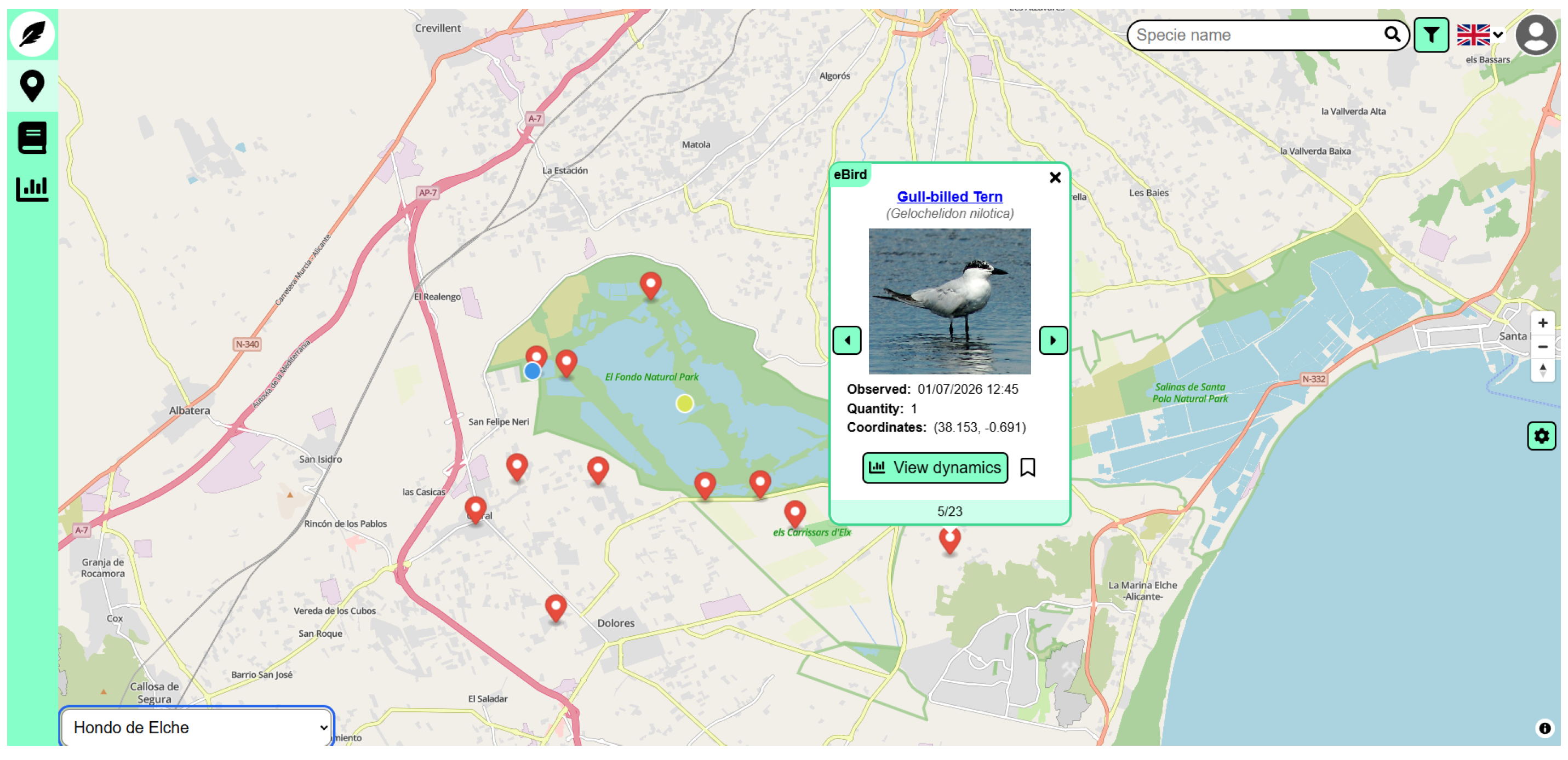
Observational records are mapped as custom geo-markers. To manage spatial overlap resulting from coincident coordinates, markers incorporate an automated spatial grouping mechanism. Interacting with a grouped marker opens a metadata view detailing species identity, detection counts, timestamps, and observational sources, as illustrated in Figure 4.

As depicted in Figure 4, each observation card provides taxonomic identifiers linked to Wikidata endpoints, detected counts, precise timestamps, and data origin tags (distinguishing between eBird, professional census, and BirdNET acoustic sensor detections). An integrated filtering panel enables querying across date ranges, observational modalities, and user-defined taxa lists, supported by a fuzzy-matching autocomplete search index spanning English, Spanish, and scientific nomenclature.

5.4. Spatiotemporal Trends and Predictive Analytics

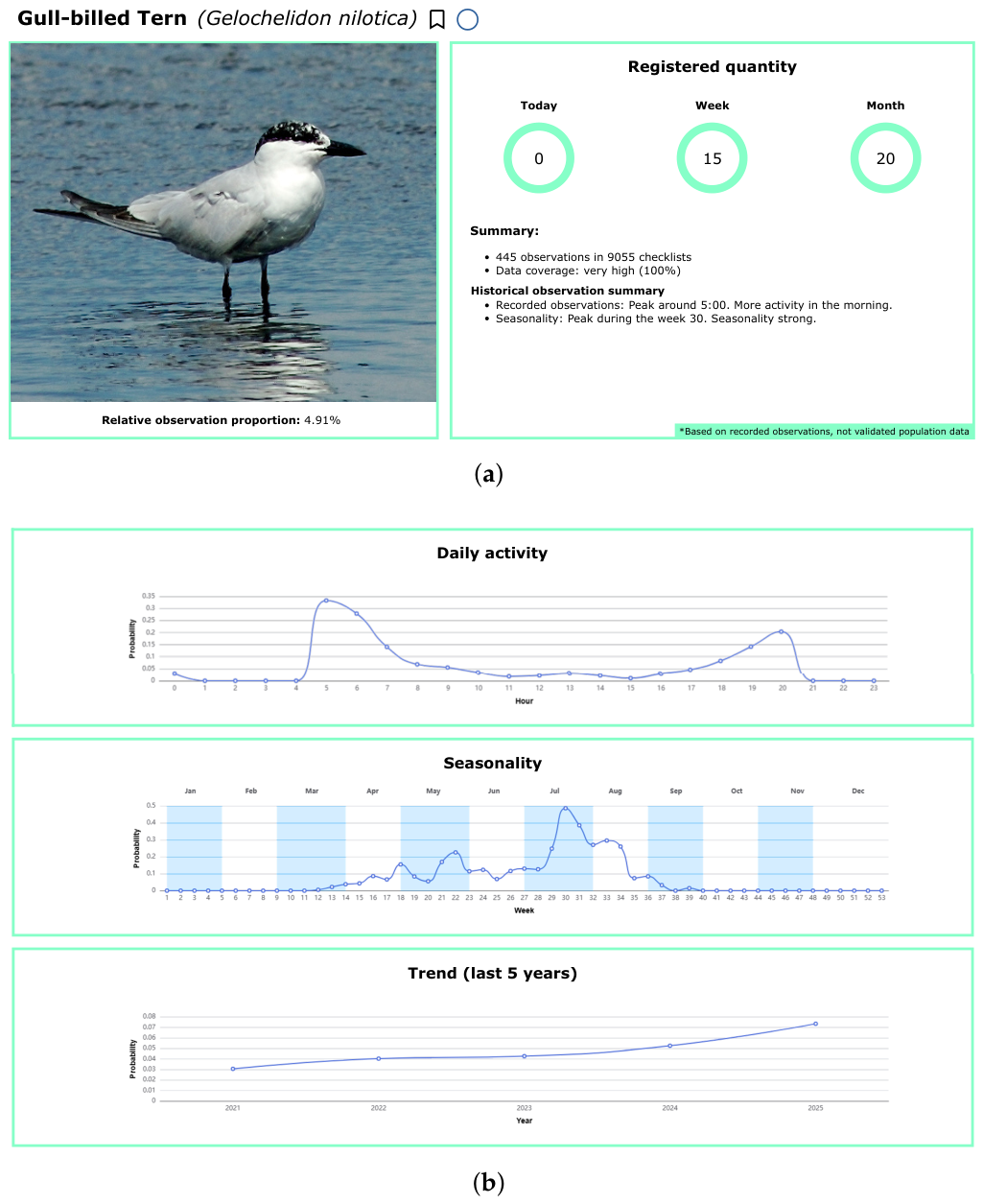
A dedicated analytics dashboard integrates historical observational metrics with predicted relative observation proportions from the deep learning models using interactive ECharts widgets [21]. Figure 5 illustrates the system output for the Gull-billed Tern (Gelochelidon nilotica).

Figure 5 shows the interface after the wording revision described in this subsection: the summary card now reads “Relative observation proportion”, “Data coverage”, and “Historical observation summary” in place of the earlier interface labels (“Probability of sighting”, “Reliability of the analysis”, “Trend: stable”), and the card adds an explicit footnote, “Based on recorded observations, not validated population data.”

As shown in Figure 5a, the platform evaluates data coverage based on observational density and sampling effort, rating the profile coverage at 100% across 9055 checklists. The summary indicates a marked early-morning peak in recorded observations, which may reflect both bird vocalisation and observer behaviour. The detailed graphical widgets in Figure 5b offer descriptive summaries rather than independently validated ecological estimates:

• Seasonality Profile: The weekly observation-proportion curve shows a summer maximum in the recorded data. The metric is 0% from January to mid-April (weeks 1–14), rises during spring, and reaches a peak of ≈0.48% during week 30 (late July), before falling back to 0% by mid-October (week 41). This pattern is compatible with seasonal presence but cannot distinguish biological phenology from variation in observation effort or detectability.
• Historical Summary (Last 5 Years): The annual plot shows an increase in the recorded relative observation proportion from ≈3% in 2021 to ≈7% in 2025. This change may reflect bird observations, checklist submission effort, detectability, or a combination of these factors; it is not evidence by itself of population recovery.

By converting model predictions into inspectable temporal distributions, the platform provides an exploratory visualization interface. For instance, querying a species during winter months yields a predicted relative observation proportion of 0.0%, which should be interpreted as a model output for the harmonised observation metric rather than proof of biological absence.

5.5. Localization and Accessibility Compliance

International accessibility is implemented via the i18next localization framework, supporting dynamic interface translation across Spanish and English. Compliance with accessibility standards is maintained in accordance with the Web Content Accessibility Guidelines (WCAG 2.1) [22], ensuring adequate contrast ratios and keyboard navigation support.

6. Discussion

6.1. Ecological Implications of Data Fusion

The common-test-set evaluation in Section 4.2 shows that adding heterogeneous bird monitoring streams does not, on aggregate, reduce prediction error for professional-census observations relative to training on census data alone; if anything, adding eBird mildly increases error for both architectures. This means the preliminary 42.7% figure reported for the recurrent LSTM (Table 5) reflected the different size and composition of the two test sets rather than a genuine benefit of augmentation. We treat this as a substantive finding about evaluation methodology in multi-source ecological data fusion, not only as a correction: apparent gains from adding large citizen-science volumes can be an artifact of evaluating on a test set that the added source itself dominates, and this should be checked explicitly in similar studies rather than assumed.

The picture is more favourable, and more interesting, for the taxa conservation practice is most concerned with. For the 50-taxon Annex I subset (Section 4.5), multi-source augmentation reduces LSTM MSE by 29% and MLP MSE by 9% relative to census-only training. We interpret this as consistent with a data-sparsity mechanism rather than a bias-correction mechanism: rare or infrequently censused species have little historical signal in professional-census records alone, so additional citizen-science context has more room to help, whereas already-common, well-sampled species see no such benefit and may even be diluted by it. This distinction—data sparsity versus source-specific observation bias—should be drawn explicitly, and the evidence here supports treating them separately rather than describing augmentation as a general bias-reduction mechanism.

While professional censuses provide highly standardized abundance estimates, their coarse temporal frequency (typically monthly) fails to capture rapid migratory passages or short-term ecological responses. Conversely, citizen science records offer dense spatial and temporal coverage but suffer from observer variance and non-standardized effort, whereas passive acoustic monitoring provides continuous, non-intrusive local detections. These differences in observation and detection processes remain present in the unified data, and the common-test result above shows they are not resolved simply by combining sources numerically.

The LSTM’s advantage over the MLP under longer temporal windows (Section 4, Table 8) is consistent with a regularizing effect of additional temporal context, but the window comparison is confounded by shrinking sample size at longer windows and does not by itself establish that the model captures migration or population dynamics. The current analysis does not establish that these predictions represent biologically realistic migration or population dynamics.

6.2. Current Dataset Limitations

Despite the success of our baseline models, several limitations within the ValWet-Birds dataset and processing pipeline present clear opportunities for refinement:

• Acoustic Sensor Spatial Sparsity: In our current dataset, the Raspberry Pi 5 audio sensor detections are statically mapped to the El Hondo–La Reserva sub-region. While the physical sensor was indeed located in this sector, its detection radius may cover adjacent zones, and the absence of localized coordinates in the raw audio metadata prevents precise spatial mapping.
• Citizen Science Count Noise: eBird checklists contain entries without count estimation. In our preprocessing pipeline, these are conservatively treated as 1 individual. While this prevents losing presence data, it introduces a downward bias in abundance calculations for common species. Additionally, the volunteer-based nature of eBird leads to spatial clustering near public access paths, leaving remote areas under-sampled.
• Environmental Vulnerability of IoT Nodes: Autonomous monitoring in wetland environments is vulnerable to extreme weather. Deployed sensors at El Hondo experienced hardware failures due to seasonal flooding in late 2024, leading to data gaps in the audio detection timeline. Fusing satellite-based flood models could help adjust for these sensor downtime periods.
• Hypersalinity and Data Sparsity: The Laguna de Torrevieja sub-region is hypersaline and supports very little birdlife. The harmonised dataset contains 921 species–month records for this sub-region (697 from eBird, 224 from Census); this is a count of aggregated species-by-month rows, not of raw eBird checklists submitted in the field, and should not be read as a raw-observation count. We distinguish checklists, observations, and harmonised dataset records explicitly here and in Section 2.6; the pre-aggregation eBird checklist log for this sub-region specifically was not available to us to report as a separate count. Prediction models for this sub-region are heavily dependent on sparse census data, leading to higher prediction uncertainty.
• Relative Observation Normalization: By normalising observation counts per source, we prevent raw count scale conflicts. However, this means the target variables are relative rather than absolute and do not correct source-specific detectability. If a user requires a single combined absolute density estimate, they must re-aggregate and scale the raw count columns manually; such an estimate would additionally require effort and detection modeling.

6.3. Future Research Directions

Future work will focus on expanding this multi-source framework along three main axes. First, visual deep learning models (e.g., YOLO-based object detectors) deployed on observatory cameras will be integrated to complement acoustic sensing with behavioral and visual verification. Second, explicit zero-inflated spatiotemporal occupancy frameworks [23] will be explored to formally model detection probabilities and account for species unobservability. Finally, future deployment efforts will scale the existing solar-powered IoT hardware architecture by establishing new sensor grid instances across additional protected wetland parks, thereby expanding spatial coverage and continuous data acquisition.

7. Conclusions

This study introduced ValWet-Birds, a unified spatiotemporal dataset and data fusion framework that harmonizes professional censuses, citizen science records (eBird), and autonomous passive acoustic monitoring (BirdNET) to model avian observation patterns across three protected wetlands in the Valencian Community, Spain. By defining a unified monthly relative observation proportion target, the methodology places heterogeneous records on a common numerical scale, but it does not make their observation processes ecologically equivalent.

A preliminary, non-matched-test comparison suggested a 42.7% lower Test Mean Squared Error for the recurrent LSTM under multi-source augmentation. Re-evaluating every source condition on an identical set of held-out professional-census observations shows that this aggregate benefit does not hold: augmentation does not reduce error relative to census-only training when all taxa are considered together; the original comparison conflated data augmentation with a change in test-set composition. However, for a 50-taxon subset cross-referenced against Annex I of the EU Birds Directive, augmentation does reduce error substantially (29% for the LSTM, 9% for the MLP), plausibly because these less-common taxa have sparser census history for the model to draw on. Both MLP and LSTM baselines clearly outperform naive temporal reference predictors on the same common test, which supports the value of the modeling approach independent of the augmentation question. None of these results confirm recovery of seasonal migration dynamics or subtle shifts in species distribution.

To support inspection of predictive modeling outputs, we deployed Avistory, an open-source web platform that translates model inferences into spatial visualization tools for researchers and other users. The platform is not presented as a validated conservation decision-support system: observed patterns and model-derived proportions can be affected by sampling effort and detectability and should not be read as population trends without ecological validation. Future developments will focus on effort-aware observation models, occupancy or detection-probability modeling, expanded sensing infrastructure with weather-hardened edge nodes, and incorporation of visual computer vision models.

References

1. IPBES. Global Assessment Report on Biodiversity and Ecosystem Services; IPBES: Bonn, Germany, 2019. [Google Scholar]
2. Kleijn, D.; Cherkaoui, I.; Goedhart, P.W.; van der Hout, J.; Lammertsma, D. Waterbirds increase more rapidly in Ramsar-designated wetlands than in unprotected wetlands. J. Appl. Ecol. 2014, 51, 289–298. [Google Scholar] [CrossRef] [Scilit]
3. Gregory, R.D.; Noble, D.; Field, R.; Marchant, J.; Raven, M.; Gibbons, D. Using birds as indicators of biodiversity. Ornis Hung. 2003, 12, 11–24. [Google Scholar]
4. Matthews, G.V.T. The Ramsar Convention on Wetlands: Its History and Development; Ramsar Convention Bureau: Gland, Switzerland, 1993. [Google Scholar]
5. Zacharias, I.; Zamparas, M. Mediterranean temporary ponds. A disappearing ecosystem. Biodivers. Conserv. 2010, 19, 3827–3845. [Google Scholar] [CrossRef] [Scilit]
6. Gregory, R.D.; Gibbons, D.W.; Donald, P.F. Bird census and survey techniques. In Bird Ecology and Conservation: A Handbook of Techniques; Sutherland, W.J., Newton, I., Green, R.E., Eds.; Oxford University Press: Oxford, UK, 2004; pp. 17–56. [Google Scholar]
7. Kamp, J.; Oppel, S.; Heldbjerg, H.; Nyegaard, T.; Donald, P.F. Unstructured citizen science data fail to detect long-term population declines of common birds in Denmark. Divers. Distrib. 2016, 22, 1024–1035. [Google Scholar] [CrossRef] [Scilit]
8. Sullivan, B.L.; Wood, C.L.; Iliff, M.J.; Bonney, R.E.; Fink, D.; Kelling, S. The eBird enterprise: An integrated approach to development and application of citizen science. Biol. Conserv. 2014, 169, 31–40. [Google Scholar] [CrossRef] [Scilit]
9. Fink, D.; Auer, T.; Johnston, A.; Ruiz-Gutiérrez, V.; Hochachka, W.M.; Kelling, S. Modeling avian full annual cycle distribution and population trends with citizen science data. Ecol. Appl. 2020, 30, e02056. [Google Scholar] [CrossRef] [Scilit] [PubMed]
10. Chandler, M.; See, L.; Copas, K.; Bonde, A.M.; López, B.C.; Danielsen, F.; Legind, J.K.; Masinde, S.; Miller-Rushing, A.J.; Newman, G.; et al. Contribution of citizen science towards international biodiversity monitoring. Biol. Conserv. 2017, 213, 280–294. [Google Scholar] [CrossRef] [Scilit]
11. Johnston, A.; Hochachka, W.M.; Strimas-Mackey, M.E.; Ruiz-Gutierrez, V.; Robinson, O.J.; Miller, E.T.; Auer, T.; Kelling, S.T.; Fink, D.; Fourcade, Y. Analytical guidelines to increase the value of community science data: An example using eBird data to estimate species distributions. Divers. Distrib. 2021, 27, 1265–1277. [Google Scholar] [CrossRef] [Scilit]
12. Isaac, N.J.B.; Pocock, M.J.O. Bias and information in biological records. Biol. J. Linn. Soc. 2015, 115, 522–531. [Google Scholar] [CrossRef] [Scilit]
13. Kellner, K.F.; Swihart, R.K. Accounting for imperfect detection in ecology: A quantitative review. PLoS ONE 2014, 9, e111436. [Google Scholar] [CrossRef] [Scilit] [PubMed]
14. Guillera-Arroita, G. Modelling of species distributions, range dynamics and communities under imperfect detection: Advances, challenges and opportunities. Ecography 2017, 40, 281–295. [Google Scholar] [CrossRef] [Scilit]
15. Kahl, S.; Wood, C.M.; Eibl, M.; Klinck, H. BirdNET: A deep learning solution for avian diversity monitoring. Ecol. Inform. 2021, 61, 101236. [Google Scholar] [CrossRef] [Scilit]
16. Pérez-Granados, C.; Traba, J. Estimating bird density using passive acoustic monitoring: A review of methods and suggestions for further research. Ibis 2021, 163, 765–783. [Google Scholar] [CrossRef] [Scilit]
17. Isaac, N.J.B.; Jarzyna, M.A.; Keil, P.; Dambly, L.I.; Boersch-Supan, P.H.; Browning, E.; Freeman, S.N.; Golding, N.; Guillera-Arroita, G.; Henrys, P.A.; et al. Data Integration for Large-Scale Models of Species Distributions. Trends Ecol. Evol. 2020, 35, 56–67. [Google Scholar] [CrossRef] [Scilit] [PubMed]
18. Delany, S. Guidelines for Participants in the International Waterbird Census (IWC); Technical Report; Wetlands International: Ede, The Netherlands, 2005. [Google Scholar]
19. MapLibre GL JS Contributors. MapLibre GL JS: Open-Source Vector Map Library. 2026. Available online: https://maplibre.org/maplibre-gl-js/ (accessed on 25 July 2026).
20. MapTiler. MapTiler: Cloud Map Services and Vector Style Editor. 2026. Available online: https://www.maptiler.com/ (accessed on 25 July 2026).
21. The Apache Software Foundation. Apache ECharts: A Powerful, Interactive Charting and Data Visualization Library. 2026. Available online: https://echarts.apache.org/ (accessed on 25 July 2026).
22. World Wide Web Consortium (W3C). Web Content Accessibility Guidelines (WCAG) 2.1. 2018. Available online: https://www.w3.org/TR/WCAG21/ (accessed on 25 July 2026).
23. MacKenzie, D.I.; Nichols, J.D.; Lachman, G.B.; Droege, S.; Andrew Royle, J.; Langtimm, C.A. Estimating site occupancy rates when detection probabilities are less than one. Ecology 2002, 83, 2248–2255. [Google Scholar] [CrossRef]
Figure 1. Location of the 12 survey units across the three study wetlands, shown on a basemap for geographic context. Each point is the mean eBird hotspot coordinate for that survey unit, colour-coded by wetland. Official polygon boundaries for the three protected areas were not available to us, so unit positions are represented by these point locations rather than by mapped park boundaries.
Applsci 16 09584 g001
Figure 2. Distribution of observations across the 12 sub-regions. Color-grouped by wetland: El Hondo (blue), Santa Pola (warm tones), and La Mata–Torrevieja (purple).
Applsci 16 09584 g002
Figure 3. Species dominance by total individuals recorded, after the taxonomic audit. The top 10 resolved species account for 53.9% of all counted individuals; 45 genus/family-level or slash-notation taxa (5.0% of individuals) are shown separately as unresolved rather than assigned to the ranking; the remaining 339 resolved species share the rest.
Applsci 16 09584 g003
Figure 4. Main interactive map interface of the Avistory application centered on the El Hondo Natural Park. Red marker pins display bird observations across different sub-regions. The active pop-up card shows detailed metadata for a clicked sighting of the Gull-billed Tern (Gelochelidon nilotica) recorded via eBird, including date, count, and precise coordinates, along with options to view dynamic trends or save the species.
Applsci 16 09584 g004
Figure 5. Dynamic statistics and spatiotemporal visualizations for the Gull-billed Tern (Gelochelidon nilotica) in Avistory: (a) The upper summary card displaying a 4.91% global relative observation proportion, registered quantity rings (today, week, month), and a summary box analyzing 445 observations in 9055 checklists, with observation-based temporal summaries. (b) The lower dashboard displaying interactive charts of recorded time-of-day observations, a weekly seasonality profile peaking at week 30, and a 5-year historical observation-proportion summary from 2021 to 2025.
Applsci 16 09584 g005