Observability-Aware Estimation of Tradeable Vehicle-to-Grid Capacity from Heterogeneous Charger Telemetry

Featured Application

The framework provides an upstream safe-capacity layer for vehicle-to-grid aggregators: it converts whatever telemetry a charging station exposes into a conservative, market-usable energy and power commitment, or into an explicit refusal to bid, and prices poor charger observability as a quantified capacity haircut that can inform metering and procurement decisions for charging infrastructure.

Abstract

Vehicle-to-grid (V2G) aggregators must commit energy and power that connected vehicles can actually deliver, yet they often observe only charger-side telemetry, and vehicle-reported state of charge (SOC) is optional or non-authoritative. This paper proposes an observability-aware framework for estimating tradeable V2G capacity: each session is classified by its measurement boundary, channels, sampling, latency, and setpoint control, then mapped to the battery through uncertain conversion paths. The estimator outputs conservative safe energy and safe power rather than absolute SOC, treats vehicle-reported values as noisy hints, and abstains when observability is insufficient. A reproducible synthetic study shows that regularization and a split-conformal margin bring the bound to the 95% target with a finite-sample guarantee under within-regime exchangeability, and that the required capacity haircut grows from about 2.6 through 4.3 to 6.5 SOC points as observability degrades. Coverage alone does not distinguish the method, since any conformalized predictor reaches the target; the observability-aware bound adds tradeable capacity at that coverage, and its advantage grows as telemetry degrades. End-to-end market deliverability is established only in synthesis: a laboratory proof of concept on one bidirectional charger with four production vehicles demonstrates AC-boundary telemetry ingestion and capability assignment, but measures realized throughput after the fact rather than a bound committed before dispatch.

1. Introduction

Vehicle-to-grid (V2G) aggregation converts parked electric vehicles (EVs) into distributed flexible resources, and a decade of research and demonstration projects has established its potential for frequency regulation, peak shaving, and renewable integration [1]. Controlled bidirectional charging can simultaneously reduce a user’s charging cost and provide measurable power-system benefit [2]. For an aggregator, the relevant operational variable is not the exact battery state of charge (SOC) of each vehicle, but the energy and power that can be committed without violating telemetry, user, charger, or market constraints. Overestimated capacity creates non-delivery and imbalance risk. Underestimated capacity leaves flexibility unused. The economic value of an aggregated portfolio depends on how conservatively, yet how accurately, per-session deliverable capacity can be inferred from the data the aggregator actually observes.

A V2G aggregator usually does not have direct access to battery-management-system (BMS) measurements such as cell voltages, pack current, battery temperature, or internal SOC estimates. The available data are often charger-side or backend measurements: AC or DC power, imported and exported energy registers, voltage and current measurements, setpoints, response behaviour, connector state, Open Charge Point Protocol (OCPP) MeterValues, local Modbus registers, vendor application programming interfaces, or external metering. Vehicle-reported SOC and capacity may be optional, delayed, rounded, biased, or lost in the EV–electric-vehicle-supply-equipment (EVSE)–backend chain. Reported SOC is not a safe runtime authority for market-facing V2G aggregation.

The consequence is asymmetric. In reserve and balancing products, committing energy or power that is not delivered triggers imbalance penalties and can disqualify the resource, whereas committing too little simply forgoes revenue; electric-vehicle-aggregator studies quantify this non-performance risk and its penalty exposure in frequency-regulation and reserve markets [3]. A real fleet is also heterogeneous: chargers expose different channels at different rates, and, as shown in Section 5, the same charger drives different vehicles to markedly different operating points. A fleet-average capacity or a single nominal rating cannot represent what an individual connected vehicle can safely deliver in the next dispatch interval. An aggregator needs a per-session decision that maps the telemetry actually available for that session into a conservative, reliability-targeted commitment—or an explicit refusal to bid when the telemetry cannot support one.

This paper addresses the charger-observability problem. Given heterogeneous charger telemetry, the task is to determine which tradeable V2G quantities are observable, which quantities require priors or anchors, and when the estimator must return zero tradeable capacity. The proposed framework does not claim calibrated absolute-SOC estimation from charger telemetry. It estimates conservative tradeable quantities, denoted $E_{\mathrm{safe}}$ and $P_{\mathrm{safe}}$, under explicit assumptions on measurement topology, conversion-path uncertainty, auxiliary load, calibration, and validation anchors.

Charger capability is classified by measurement boundary, available channels, sampling rate, command latency, and setpoint controllability. A DC charger observed only through slow AC-side OCPP energy registers is less informative than the same charger observed through fast DC voltage, current, and energy telemetry. An AC wallbox with reliable active-power and energy measurements can support AC-boundary energy accounting and availability checks, but it cannot expose battery-side impedance information. Treating all chargers as a single homogeneous data source hides the dominant source of capacity uncertainty.

This paper makes three main contributions.

• Observability-aware identifiability and a measurement-topology model. A capability taxonomy classifies each charger session by measurement point, channels, sampling rate, latency, and setpoint control, coupled to a measurement-to-battery conversion-path model with condition-dependent efficiencies and explicit auxiliary load; an identifiability analysis establishes which tradeable quantities are recoverable from boundary telemetry and which require anchors.
• Conservative tradeable-capacity estimation with abstention. A conservative-quantile estimator with held-out calibration treats vehicle-reported SOC and capacity as noisy hints and outputs calibrated lower bounds $E_{\mathrm{safe}}/P_{\mathrm{safe}}$, or abstains when observability or calibration is insufficient. Every coverage number reported here comes from this static Monte Carlo read-out (Algorithm A1), which is the estimator actually evaluated. The sequential particle filter (Algorithm 1) is the extension that assimilates SOC hints when a session provides them; in the no-hint regime studied here it reduces to the same read-out, and it is run end-to-end only to confirm that its assimilation and resampling machinery fires and is no less conservative—not to claim an accuracy gain over the static estimator, which this paper does not demonstrate.
• An observability-priced haircut, in synthesis and hardware. A reproducible synthetic study (coverage, model-mismatch, sensitivity, calibration-size, reliability, and baseline sub-studies) quantifies how the required conservative haircut grows as observability degrades, and a laboratory AC-boundary proof-of-concept on a bidirectional combined-charging-system (CCS) charger with four production EVs shows charger-limited V2G export and vehicle-dependent import, supporting per-session over single-rating capability assignment.

Coverage calibration is used as an engineering ingredient rather than claimed as a novel method (Section 2); the distinct claim is the integration of measurement-topology-aware identifiability, conservative tradeable output, and abstention into a single safe-capacity layer calibrated per capability regime, as contrasted with the closest prior work in Table 1.

Section 2 reviews related work and identifies the gap. Section 3 formalizes the observability problem and the identifiability of battery state from boundary telemetry. Section 4 presents the safe-capacity estimation framework, including the measurement-to-battery path model, the runtime estimator, and coverage calibration. Section 5 reports the synthetic coverage study and the hardware-in-the-loop proof of concept. Section 6 discusses limitations and concludes. Symbols are collected in the Nomenclature at the end of the paper.

2. Related Work and Gap

2.1. State and Capacity Estimation from Battery or External Measurements

Battery-side SOC and state-of-health estimators typically use pack or cell voltage, current, temperature, open-circuit-voltage–SOC relations, equivalent-circuit models, or learned BMS signals. These signals are not generally available to a charger-only V2G aggregator. External-measurement approaches are closer to the present problem. Najar et al. estimate SOC from smart-plug point-of-common-coupling measurements using a data-driven model [4]. Pasetti et al. estimate SOC of light electric vehicles from active power measured at the charging socket after offline characterization of a battery/charger set [5]. Zakharov et al. estimate EV battery capacity from real-world charging traces using spectral learning, but the dataset includes pack-level telemetry such as SOC, voltage, current, and temperature [6]. Within the BMS context, particle-filter and unscented-particle-filter estimators are well established for SOC, state-of-energy, and remaining-useful-life estimation under nonlinear, non-Gaussian dynamics [7,8,9,10,11]; the present work adopts this filtering machinery but applies it at the charger-observability boundary rather than to pack-level signals. The overlap is limited to state or capacity inference. These methods do not provide a measurement-topology-aware V2G safe-capacity estimator across heterogeneous EVSE telemetry, and they do not output calibrated tradeable $E_{\mathrm{safe}}/P_{\mathrm{safe}}$ with abstention.

2.2. EVSE Data, Flexibility Forecasting, and Aggregate Storage Models

EVSE and charging-session data have been used for flexibility forecasting and aggregate storage abstraction. The Adaptive Charging Network provides large-scale EVSE monitoring and control and documents practical limits such as quantized control signals, non-ideal charging behaviour, and unbalanced infrastructure [12]. Pertl et al. model aggregated EVSE demand as an equivalent time-variant storage system [13]. Genov et al. forecast charging flexibility from session data and show that user-provided energy and parking-duration inputs can be unreliable [14]. Ko et al. assess EV2G flexibility from historical charger records using probabilistic charger profiles and a virtual EV2G model [15]. Jokinen and Lehtonen quantify the power-system benefit and cost reduction achievable when EV charging is coordinated with demand response and V2G [2], and a recent decade-scale review consolidates the achievements and open challenges of V2G deployment [1]. This literature treats EVSE data as a forecasting or aggregation input. It does not model runtime measurement topology, conversion-path uncertainty, or per-session calibrated $E_{\mathrm{safe}}/P_{\mathrm{safe}}$.

2.3. Aggregate Flexibility, Dispatchable Regions, and Robust Bidding

Aggregate-flexibility models characterize feasible EV operation once per-vehicle constraints are specified. Schlund et al. propose FlexAbility for modelling bidirectional flexibility from large pools of unidirectional EV charging loads [16]. Zhou et al. form dispatchable regions for EV aggregation in microgrid bidding, using power and cumulative-energy limits [17]. Li and Li propose a distributionally robust method for real-time EV flexibility evaluation under uncertain departure behaviour and SOC [18]. Ke et al. maximize intra-day V2G feasible capacity by coupling traffic-flow modelling with prospect theory, so that the capacity an aggregator can count on reflects where vehicles actually travel and how their owners subjectively weigh incentives against range risk [19]. That work and this one are complementary: they bound the same market quantity from two different directions. Ke et al. resolve which vehicles will be connected, for how long, and with what willingness to discharge, the mobility and behavioural uncertainty upstream of the plug, while treating each connected vehicle’s energy content as known. This paper takes connection and willingness as given and resolves what remains uncertain after the plug: whether the charger telemetry of an already-connected session can support a defensible energy bound at all. The two uncertainties compound in deployment, and a fleet-level feasible-capacity figure computed from behavioural models still inherits the per-session observability haircut quantified here. Mukhi et al. construct robust aggregate flexibility sets with probabilistic guarantees under uncertain charging requirements [20]. García-Cerezo et al. build stochastic adaptive robust day-ahead bidding curves for a V2G aggregator [21]. These methods operate downstream of the telemetry layer. They assume, forecast, or bound EV constraints. They do not infer those constraints from heterogeneous charger measurements.

2.4. Calibrated Flexibility Guarantees

Calibrated and conformal uncertainty quantification has been applied to aggregate flexibility. Pipada Sunil Kumar et al. combine Monte Carlo dropout and conformal prediction to produce calibrated prediction intervals for prosumer flexibility in ancillary-service markets, addressing P90 compliance and overbidding risk [22]. Distribution-free conformal methods more broadly provide finite-sample coverage guarantees without distributional assumptions [23], including conformalized quantile regression for calibrated one-sided bounds [24], and have been applied to calibrated interval forecasting of electricity prices and renewable power [25,26]. The present paper does not claim calibrated prediction as a standalone contribution. Calibration is applied at the charger-observability layer, where heterogeneous telemetry is converted into conservative per-session $E_{\mathrm{safe}}/P_{\mathrm{safe}}$.

2.5. V2G Efficiency, Measurement Boundary, and Charger Dynamics

Empirical studies of V2G efficiency and charger dynamics motivate the conversion-path model. Apostolaki-Iosifidou et al. measure EV charging and discharging losses and report strong dependence on power level, SOC, direction, and power-electronics conversion stages [27]. Schram et al. report V2G round-trip efficiencies affected by current rate, ambient temperature, and SOC, with configurations that include charger-side and onboard AC/DC conversion [28]. Zecchino et al. characterize commercial CHAdeMO V2G chargers in terms of efficiency, activation time, response granularity, ramping, accuracy, and precision [29]. Pedersen et al. compare CCS2 and CHAdeMO bidirectional charger response dynamics and show that local response, ramping, and power-flow reversal delays are essential for grid-service validation [30]. These measurements show that efficiency and response cannot be represented by a single constant or by the nominal charger rating alone. The proposed estimator propagates boundary, conversion-path, and response uncertainty into the safe-capacity output.

2.6. Protocol Observability and Vehicle-Reported SOC

Standards-based communication does not guarantee trustworthy backend observability. Charger communication protocols are fragmented: multiple open and proprietary protocols (OCPP, OSCP, ISO 15118) offer limited interoperability [31,32], and even operator roaming relies on several mutually incompatible protocols [33], reinforcing the measurement-boundary heterogeneity the taxonomy classifies. Rahman et al. show that optional SOC reporting in OCPP 2.0.1 can be spoofed and can affect scheduling and station occupancy [34]. Heinekamp et al. implement a standards-based smart-charging architecture and report discrepancies between setpoints and actual measurements [35]. These results motivate the non-authoritative treatment of vehicle-reported SOC and capacity in the proposed estimator.

2.7. Gap

Existing work covers external SOC estimation, battery-capacity inference from charging traces, EVSE flexibility forecasting, equivalent-storage modelling, robust EV flexibility, bidding under uncertainty, calibrated aggregate flexibility, V2G efficiency, and charger response dynamics. These strands do not jointly address the charger-observability problem faced by a V2G aggregator. Given heterogeneous EVSE/backend telemetry with different measurement boundaries, channels, sampling rates, latencies, and controllability, the missing layer is a method that determines conservative tradeable energy and power when vehicle-reported SOC and capacity are non-authoritative. This paper addresses that layer with a measurement-topology-aware conversion-path model and a coverage-calibrated estimator that outputs $E_{\mathrm{safe}}/P_{\mathrm{safe}}$ or abstains. Table 1 contrasts this integration with the closest prior work along the axes that distinguish it: the input actually assumed, whether a per-session abstention path exists, and whether calibration is tracked per observability/capability regime.

Table 1. Positioning versus the closest prior work. Abst.: per-session abstention path; Per-Reg. Cal.: calibration tracked per observability/capability regime. Bold marks the present work.

Approach	Primary Input	Abst.	Per-Reg. Cal.
External-meas. SOC [4,5]	AC power at plug/PCC	No	No
Flexibility from records [14,15]	Session/charger history	No	No
Robust EV flexibility [18,20]	Assumed/forecast constraints	No	No
Calibrated flexibility [22]	Prosumer flex. series	No	No
This work	Heterogeneous charger telemetry	Yes	Yes

Table 1. Positioning versus the closest prior work. Abst.: per-session abstention path; Per-Reg. Cal.: calibration tracked per observability/capability regime. Bold marks the present work.

Approach	Primary Input	Abst.	Per-Reg. Cal.
External-meas. SOC [4,5]	AC power at plug/PCC	No	No
Flexibility from records [14,15]	Session/charger history	No	No
Robust EV flexibility [18,20]	Assumed/forecast constraints	No	No
Calibrated flexibility [22]	Prosumer flex. series	No	No
This work	Heterogeneous charger telemetry	Yes	Yes

3. Problem Setting and Observability

3.1. Measurement References and State Anchors

The term “ground truth” is avoided. A measurement reference validates a physical electrical quantity at a defined boundary. It does not automatically validate battery internal state. A state anchor constrains battery state. A PQube analyzer at the AC boundary is a measurement reference for AC power and energy, not an SOC anchor. A BMS/CAN SOC value logged outside the runtime estimator is a field anchor with uncertainty, not an authoritative truth. A strong exogenous anchor requires independence from the runtime pipeline and from the vehicle SOC logic, with bounded endpoint, boundary, throughput, path-efficiency, and auxiliary-load uncertainty.

3.2. Telemetry Sanity Checks and Capability Assignment

Before estimation, each session passes through a telemetry sanity layer. The layer checks power-flow sign convention using signed power and energy registers, classifies the measurement boundary as AC-side, DC-side, vehicle-reported, or unknown, estimates timestamp offset and drift when multiple streams are available, and checks import/export register consistency against integrated signed power. Sessions with unresolved direction, timing, or measurement-boundary conflicts are downgraded in capability class or assigned to abstention.

A charger session is assigned a capability class from

$$\mathcal{C}=f(M,X,S,L,U),$$

(1)

where M is the measurement boundary, X is the set of available channels, S is the sampling class, L is the command and measurement latency profile, and U denotes setpoint controllability. The resulting classes and the outputs each admits are listed in

Table 2. Representative capability classes and admissible outputs.

Class	Telemetry	Admissible Outputs/Tests
C	Directional energy, slow sampling	Energy ledger; conservative $E_{\mathrm{safe}}$; high uncertainty
B-AC	AC-boundary $P/E$ and status or setpoint	AC energy; availability/tracking; no battery $\Delta V/\Delta I$
A-DC	DC-output $V/I/P/E$ and setpoint	Energy; $\Delta V/\Delta I$; $R_{\mathrm{proxy}}$; limited SOC refinement
A+	Fast synchronized DC or multi-vantage telemetry	Stage closure; probing; reduced conversion uncertainty
D	Missing direction, timestamps, or boundary	Abstain

. A session with AC-boundary power and energy but no DC-side voltage/current supports AC-boundary energy integration and availability checks. It does not support battery-side $\Delta V/\Delta I$, $R_{\mathrm{proxy}}$, or open-circuit-voltage-proxy diagnostics. The axes are used with indicative thresholds: “slow” sampling denotes per-transaction energy registers or sub-$0.1$ Hz updates and “fast” denotes $\gtrsim 1$ Hz aligned streams; “reliable timestamps” means cross-stream drift below the integration tolerance (e.g., <1 s over a session); and the latency profile L summarizes command-to-actuation delay (typically seconds for OCPP setpoints).

Table 3. Representative interface-to-capability mapping.

Interface	Typical Channels	Likely Class
OCPP 2.0.1 MeterValues	Slow E, optional SOC	C or B-AC
AC wallbox Modbus	$P,E$, status, setpoint	B-AC
DC charger Modbus/API	DC $V,I,P,E$, setpoint	A-DC
ISO 15118-20 + DC meter	DC telemetry, fast	A-DC/A+
Vehicle-reported only	SOC (optional)	D (anchor only)

maps representative interfaces—including OCPP 2.0.1 backend telemetry [36] and the ISO 15118-20 bidirectional-power-transfer interface [37]—to their likely capability classes.

3.3. Identifiability and Anchorability

Over an interval $[t_0,t_1]$, charger telemetry yields signed metered power $P_m\left(t\right)$ and measured throughput $\Delta E_m=\int P_m\left(t\right)dt$, decomposed into charging and discharging components $\Delta E_m^{+}$ and $\Delta E_m^{-}$. The battery-side increment is modelled as

$$\Delta E_{\mathrm{batt}}=H_{\mathrm{ch}}\Delta E_m^{+}-{\displaystyle \frac{\Delta E_m^{-}}{H_{\mathrm{dis}}}}-\int P_{\mathrm{aux}}\left(t\right)dt,$$

(2)

where $H_{\mathrm{ch}}$ and $H_{\mathrm{dis}}$ are condition-dependent path efficiencies and $P_{\mathrm{aux}}$ is auxiliary load. One boundary convention is used throughout the paper. $P_{\mathrm{aux}}$ is a battery-side load in kW, the vehicle’s own auxiliary and thermal demand [38], so it is subtracted from the battery-side energy and is not referred to the AC boundary. The meter bias b introduced in Section 4.3 is an AC-boundary quantity, since it is an error of the charger-side meter. Under this convention the energy a discharge delivers to the AC boundary is $\left(\Delta E_{\mathrm{batt}}^{\mathrm{out}}-\int P_{\mathrm{aux}}dt\right)H_{\mathrm{dis}}$: the auxiliary draw is taken from the pack first, and only the remainder is converted. Appendix C states the closed form used by the synthetic generator, which follows this same ordering. The state relation is

$$SOC\left(t_1\right)=SO{C}_0+100{\displaystyle \frac{\Delta E_{\mathrm{batt}}}{E_{\mathrm{usable}}}}.$$

(3)

The local identifiability of $(SO{C}_0,E_{\mathrm{usable}})$ can be examined through the rank of the observation Jacobian, in the sense of structural identifiability [39]. For a single SOC-like observation $y=h\left(SOC\left(t_1\right)\right)+ϵ$, the Jacobian with respect to $(SO{C}_0,E_{\mathrm{usable}})$ is

$$J=h^{\prime }\left[1,-100{\displaystyle \frac{\Delta E_{\mathrm{batt}}}{E_{\mathrm{usable}}^2}}\right],$$

(4)

with rank at most one. The pair $SO{C}_0$ and $E_{\mathrm{usable}}$ is not jointly locally identifiable from energy-only telemetry plus one SOC-like observation. With two independent state anchors at $t_a<t_b$, the corresponding two-row Jacobian has full rank when $h_a^{\prime },h_b^{\prime }\ne 0$ and $\Delta E_b-\Delta E_a\ne 0$. The anchors then bracket nonzero battery-side throughput, and 

$$E_{\mathrm{usable}}=100{\displaystyle \frac{\Delta E_{\mathrm{batt}}}{\Delta SOC}}$$

(5)

is identifiable up to anchor, path, and auxiliary-load uncertainty. The derivation in Appendix A treats the minimal two-parameter case; in practice $H_{\mathrm{ch}},H_{\mathrm{dis}}$, the auxiliary load, and the meter bias are also unknown, so the effective identifiability problem is strictly harder and the unidentified set only widens, which further motivates abstention and exogenous state anchors. Realized boundary energy is the strongest claim tier. Battery-side energy is path-dependent. $\Delta SOC$ requires bounded capacity. Calibrated absolute SOC requires a level anchor.

4. Safe-Capacity Estimation Framework

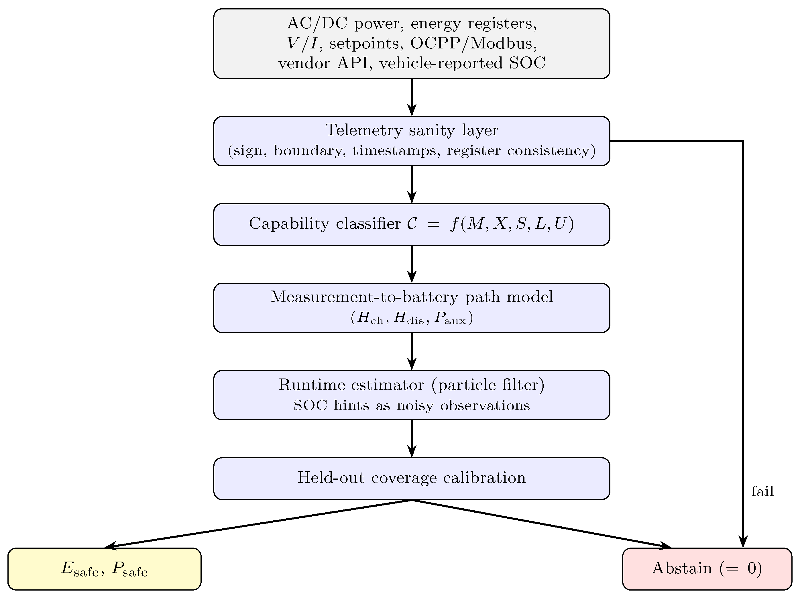
The framework is organized as a pipeline (Figure 1). Heterogeneous telemetry first passes the sanity layer, is assigned a capability class, mapped to the battery through a conversion path, processed by a runtime estimator, and finally calibrated into the conservative market-facing outputs $E_{\mathrm{safe}}/P_{\mathrm{safe}}$ or an abstention decision.

4.1. System and Market Context

The estimator is an upstream layer for a V2G aggregator that bids per-session flexibility into energy and ancillary-service markets [2,17,21]. For a dispatch horizon $\mathcal{H}$, the aggregator must commit a quantity it can deliver with high probability; non-delivery is penalized through imbalance settlement or reserve-qualification rules (e.g., the P90 requirement in several frequency-reserve products [22]), and probabilistic guarantees on real-time delivery are an established basis for storage scheduling in energy and reserve markets [40]. The per-session outputs are defined as conservative lower bounds,

$$\begin{array}{cc}\hfill Pr\left(E_{\mathrm{realized}}\ge E_{\mathrm{safe}}\right)& \ge 1-\alpha ,\hfill \\ \hfill Pr\left(P_{\mathrm{realized}}\ge P_{\mathrm{safe}}\right)& \ge 1-\alpha ,\hfill \end{array}$$

(6)

where $1-\alpha$ is the market-required reliability level. The portfolio bid is the sum of per-session $E_{\mathrm{safe}}/P_{\mathrm{safe}}$ over the non-abstaining sessions.

The term tradeable capacity is used in one narrow sense throughout. $E_{\mathrm{safe}}$ is an energy-limited bound: the AC-boundary energy a connected session can deliver before its battery reaches a fixed SOC floor, given what the charger telemetry reveals about that session. It is the quantity charger observability limits, and the only quantity this paper estimates and calibrates. Four further constraints stand between such a bound and a qualified market product, and none of them enters the estimator or its validation. Departure uncertainty and the driver’s requested departure energy shorten the horizon and raise the effective floor, so the deliverable energy is the minimum of the bound computed here and whatever the mobility constraint leaves; models of that constraint are a separate literature [18,19,20]. Activation duration and product-specific endurance requirements are not represented, since the bound is computed for a single declared horizon and not for a product’s activation profile. Ramp rate and setpoint-tracking compliance are power-path properties that the retained AC-boundary measurements cannot establish, as Section 5.7 states where $P_{\mathrm{safe}}$ is reported. What follows is an observability-limited upper layer on the tradeable quantity, not a qualified reserve offer; the remaining constraints compose with it downstream and can only reduce it. This makes the observability problem economically explicit: a larger conservative haircut (lower $E_{\mathrm{safe}}$ for the same expected energy) is the price of weaker charger telemetry.

4.2. Measurement-to-Battery Path Model

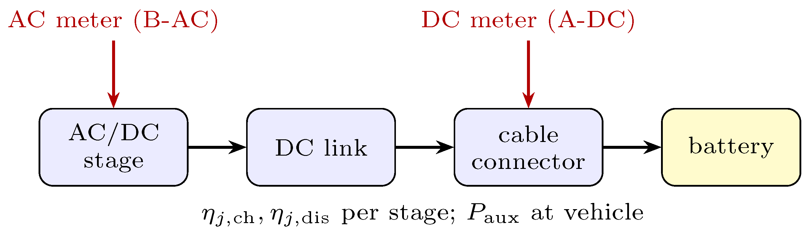
Each measurement boundary defines a path of conversion stages between the measured quantity and the battery. For AC-boundary measurements of a DC charger, the path includes the charger AC/DC stage, DC link, DC cable, connector, and battery interface. For AC V2G wallboxes, the vehicle onboard bidirectional converter is an additional unobserved stage. Each stage j has condition-dependent charge and discharge efficiencies ${\eta }_{j,\mathrm{ch}}(P,T,SOC)$ and ${\eta }_{j,\mathrm{dis}}(P,T,SOC)$, plus residual uncertainty. The aggregate path efficiencies are the products of the stage efficiencies on the selected path,

$$H_{\mathrm{ch}}=\prod _j{\eta }_{j,\mathrm{ch}},H_{\mathrm{dis}}=\prod _j{\eta }_{j,\mathrm{dis}}.$$

(7)

Shared latent factors such as temperature, power level, and SOC induce correlations across stages and auxiliary load. Figure 2 shows the conversion path and the measurement vantage points relevant to the capability classes of Table 2.

For a selected measurement path, charging and discharging energy are propagated as

$$\begin{array}{cc}\hfill E_{\mathrm{batt},\mathrm{in}}& =\int P_m^{+}\left(t\right)H_{\mathrm{ch}}\left(t\right)dt,\hfill \end{array}$$

(8)

$$\begin{array}{cc}\hfill E_{\mathrm{batt},\mathrm{out}}& =\int {\displaystyle \frac{P_m^{-}\left(t\right)}{H_{\mathrm{dis}}\left(t\right)}}dt,\hfill \end{array}$$

(9)

where $P_m^{+}\left(t\right)=max(P_m\left(t\right),0)$ and $P_m^{-}\left(t\right)=max(-P_m\left(t\right),0)$. Consistent with the energy balance (2) and the propagation law (11), the auxiliary load $\int P_{\mathrm{aux}}\left(t\right)dt$ is handled once, as a separate state-dependent term subtracted from the battery-side energy; it is not folded into $H_{\mathrm{ch}}$ or $H_{\mathrm{dis}}$.

4.3. Runtime Estimator

The runtime estimator is a sequential Monte Carlo (particle) filter [7,41], chosen because the measurement-to-battery map is nonlinear and the posterior over capacity and path parameters is generally non-Gaussian and can be multimodal, which precludes a single Gaussian (Kalman) summary. The same filtering family is standard for battery state estimation [8,9,10,11]; here it is applied at the charger boundary rather than to pack-level signals. The augmented state at step k collects the dynamic battery energy and the slowly varying static parameters,

$${\mathbf{x}}_k={\left[E_{\mathrm{batt},k},E_{\mathrm{usable}},H_{\mathrm{ch}},H_{\mathrm{dis}},P_{\mathrm{aux}},b\right]}^{\top },$$

(10)

where b is a meter bias. Here $H_{\mathrm{ch}}$ and $H_{\mathrm{dis}}$ are treated as effective session-level path efficiencies (slowly varying static parameters held constant within a session); their dependence on power, temperature, and SOC enters through the capability-conditioned prior and the shared latent factors, not through an explicit intra-session time-varying law. Battery energy is propagated from the metered power using the path model,

$$E_{\mathrm{batt},k}=E_{\mathrm{batt},k-1}+\left(H_{\mathrm{ch}}{\tilde{P}}_{m,k}^{+}-\frac{{\tilde{P}}_{m,k}^{-}}{H_{\mathrm{dis}}}-P_{\mathrm{aux}}\right)\Delta t_k+w_k,{\tilde{P}}_{m,k}=P_{m,k}-b,$$

(11)

with process noise $w_k$. The two correction terms enter at the boundary each belongs to, following the convention of Section 3: the meter bias b corrects the metered power before the conversion, so a bias of b at the AC meter costs the pack $b/H_{\mathrm{dis}}$ on the discharge leg, whereas the battery-side auxiliary load $P_{\mathrm{aux}}$ is subtracted after it. The static parameters follow a small kernel random walk (a Liu–West shrinkage move) to avoid sample impoverishment while preserving their mean [42]. When a (non-authoritative) SOC-like hint $y_k$ is available it enters only through the likelihood

$$p(y_k\mid {\mathbf{x}}_k^{\left(i\right)})\propto exp\left[-\frac{1}{2{\sigma }_y^2}{\left(y_k-h\left(SO{C}_k^{\left(i\right)}\right)\right)}^2\right],$$

(12)

and the importance weights are updated as ${\tilde{w}}_k^{\left(i\right)}\propto w_{k-1}^{\left(i\right)}p(y_k\mid {\mathbf{x}}_k^{\left(i\right)})$. The effective sample size $N_{\mathrm{eff}}={\left({\sum }_i{\left(w_k^{\left(i\right)}\right)}^2\right)}^{-1}$, with the weights normalized so that ${\sum }_i{w}_k^{\left(i\right)}=1$, triggers regularized (kernel) resampling when $N_{\mathrm{eff}}<N/2$, which mitigates particle depletion in the static-parameter subspace [43]. The market-facing quantity is read once, as a lower quantile of the final tradeable-energy distribution $G_E$ obtained by propagating each particle over the dispatch horizon, rather than by chaining lower quantiles of intermediate quantities. Algorithm 1 summarizes one estimation cycle, and Appendix B gives the per-cycle filter details. This sequential filter is exercised on the synthetic sessions in Section 5, where the SOC-hint likelihood and $N_{\mathrm{eff}}$-triggered resampling are shown to fire; the reported coverage study evaluates its lower-quantile-plus-calibration read-out through the equivalent static Monte Carlo of (13).

Algorithm 1 Runtime safe-capacity estimation cycle

1: Input: telemetry streams, capability class $\mathcal{C}$, priors, calibration map   2: Run telemetry sanity checks; resolve sign, boundary, timestamps   3: if direction, timing, or boundary unresolved then   4:     return $E_{\mathrm{safe}}=P_{\mathrm{safe}}=0$ abstain   5: end if   6: Select measurement-to-battery path from $\mathcal{C}$   7: for each timestep t do   8:     Align streams; form $P_m^{+}\left(t\right),P_m^{-}\left(t\right)$   9:     Propagate battery energy with process and static-parameter noise 10:     Apply observation likelihoods (incl. SOC hints as noisy obs.) 11:     Regularized resampling if effective sample size below threshold 12: end for 13: Form distributions of final tradeable quantities $G_E,G_P$ 14: $E_{\mathrm{safe}}\leftarrow Q_{\alpha }\left(G_E\right)$; $P_{\mathrm{safe}}\leftarrow Q_{\alpha }\left(G_P\right)$ 15: Subtract held-out calibration margin: $E_{\mathrm{safe}}\leftarrow max(E_{\mathrm{safe}}-{\kappa }^{★},0)$ (likewise $P_{\mathrm{safe}}$) 16: if ${\kappa }^{★}$ above ceiling calibration invalid then 17:     return $E_{\mathrm{safe}}=P_{\mathrm{safe}}=0$ 18: end if 19: return  $E_{\mathrm{safe}},P_{\mathrm{safe}}$

4.4. Coverage Calibration and Abstention

Bayesian filtering alone does not guarantee empirical coverage. The estimator applies a held-out calibration margin and tracks coverage by topology/capability regime. The market-facing output is

$$E_{\mathrm{safe}}=Q_{\alpha }\left(G_E(\mathsf{\Theta },\mathcal{D},\mathcal{H})\right),$$

(13)

where $G_E$ maps jointly sampled uncertain inputs $\mathsf{\Theta }$, observed data $\mathcal{D}$, and dispatch horizon $\mathcal{H}$ to realized market energy. The quantity $P_{\mathrm{safe}}$ is a lower quantile of sustainable deliverable power.

Because the filter posterior can be miscalibrated, the lower quantile is corrected on a held-out set by split conformal prediction [23,24]. Let ${\mathcal{S}}_{\mathrm{cal}}$ be a calibration set of n completed sessions in the same capability regime, and score each one by how far the bound overshot what it delivered,

$$\begin{array}{cc}\hfill {\sigma }^{\left(s\right)}& =E_{\mathrm{safe}}^{\left(s\right)}-E_{\mathrm{realized}}^{\left(s\right)},s\in {\mathcal{S}}_{\mathrm{cal}},\hfill \\ \hfill {\kappa }^{★}& =max\left({\sigma }_{\left(k\right)},0\right),k=⌈(n+1)(1-\alpha )⌉,\hfill \end{array}$$

(14)

where ${\sigma }_{\left(1\right)}\le \cdots \le {\sigma }_{\left(n\right)}$ are the ordered scores, and the deployed bound is $E_{\mathrm{safe}}\leftarrow max(E_{\mathrm{safe}}-{\kappa }^{★},0)$. Because the coverage event $E_{\mathrm{realized}}\ge E_{\mathrm{safe}}-\kappa$ is exactly $\sigma \le \kappa$, this is the standard one-sided split-conformal construction, and it carries the corresponding finite-sample distribution-free guarantee: if the calibration and test sessions of a regime are exchangeable, then

$$1-\alpha \le Pr\left(E_{\mathrm{realized}}\ge E_{\mathrm{safe}}-{\kappa }^{★}\right)\le 1-\alpha +{\displaystyle \frac{1}{n+1}},$$

(15)

for any bound-generating procedure and any underlying distribution [23,24]. Clipping ${\kappa }^{★}$ at zero keeps the margin a haircut and can only raise coverage, so it preserves the lower bound. Three qualifications bound what (15) delivers. It is a marginal statement over sessions in the regime, not a per-session one: a specific session is not certified to be covered with probability $1-\alpha$. It is finite only once the regime has enough calibration sessions, since $k\le n$ requires $n\ge 19$ at $\alpha =0.05$. It is conditional on exchangeability within the regime, so it does not survive distribution shift across regimes; Section 5.2 deliberately breaks and measures that case. Weighted and adaptive conformal methods that restore coverage guarantees under covariate and distribution shift [44,45] would harden that case and are not used here. Because $\kappa$ is in energy units, it is calibrated separately per capability regime (and, in a fleet, per battery-capacity band, so that a fixed kWh margin does not impose unequal risk on a 40 kWh and a 100 kWh pack); the haircut is reported normalized as SOC points. Calibration is tracked per topology/capability regime so that a poorly observed class cannot borrow coverage from a well observed one.

This fixes what has to be recalibrated when a charger or a vehicle model is seen for the first time. The margin is a property of the regime, the capability class of Table 2 crossed with the battery-capacity band, and not of the charger model, the vehicle model, or the pair. A previously unseen charger–vehicle combination needs no calibration of its own: it is classified by the same rules as any other session and inherits the margin already accrued for the regime it lands in. Separate calibration is required only when a combination introduces a new regime, that is, when it changes the measurement boundary, the available channels, the sampling class, or the capacity band. Regime-level pooling is the intended trade: it keeps the calibration set large enough to be usable, whereas a per-model margin would fragment the data across dozens of thin sets, none of which would reach the sample size the coverage argument needs. Two conditions bound the claim. First, the pooling is only as good as the classification: if two charger models share a capability class but differ systematically in conversion path or auxiliary load, they are not exchangeable within the regime and the pooled margin can under-cover the worse of the two, the cross-regime shift case that Section 5.2 deliberately breaks and measures. Second, a regime with too few completed sessions cannot yet certify a margin at all: the split-conformal quantile is finite only for $|{\mathcal{S}}_{\mathrm{cal}}|\ge 19$ at $\alpha =0.05$, and Section 5.5 shows the margin stays badly over-conservative well past that floor. Until a regime accrues enough sessions, the operational rule is to serve it with the margin of the most conservative regime in its capability class and, failing that, to abstain. Missing directional energy, unreliable timestamps, unknown measurement boundary, unbounded path uncertainty, or a margin ${\kappa }^{★}$ above a regime ceiling force $E_{\mathrm{safe}}=P_{\mathrm{safe}}=0$.

Table 4. Abstention conditions.

Condition	Reason	Market Action
No directional energy	Flow not observable	Do not bid
No reliable timestamps	Cannot integrate/align	Do not bid
Unbounded path uncertainty	Battery-side energy not bounded	Conservative floor or abstain
No state prior and no anchor	Absolute level unobservable	Energy-ledger mode only 1
Persistent tracking error	BMS/EVSE clipping	Reduce or withdraw
User override/departure	User priority	Remove from portfolio
Measurement conflict	Inconsistent sources	Reduce confidence or abstain
Margin above ceiling	Model unreliable in regime	Do not bid

¹ With no state prior and no anchor, the session supports only a relative battery-side energy ledger $\Delta E_{\mathrm{batt}}$: neither the absolute level nor $\Delta SOC$ is recoverable, because converting $\Delta E_{\mathrm{batt}}$ to SOC points requires $E_{\mathrm{usable}}$, which is identifiable only under the two-anchor full-rank condition of Section 3 (Equation (5)). $\Delta SOC$ mode becomes admissible one row higher in the observability ladder, once two anchors bracketing nonzero battery-side throughput are available.

lists the abstention conditions and the corresponding market actions.

4.5. Computational Complexity and Real-Time Operation

The two algorithms play different roles and are not alternatives. Algorithm 1 is the runtime per-session estimator: the sequential particle filter of Section 4 that an aggregator would run online, propagating the augmented state (11) and assimilating non-authoritative SOC hints through the likelihood (12). Algorithm A1 is the offline evaluation procedure: the static Monte Carlo of the final tradeable-energy expression (13) over jointly sampled uncertain inputs, plus the held-out calibration margin (14) fit on one split and applied to the other. Every synthetic number reported in this paper is produced by Algorithm A1: the results of Section 5.1, Section 5.2, Section 5.3, Section 5.4, Section 5.5 and Section 5.6. Algorithm 1 produces only the filtered session trajectory and the cross-check reported in Section 5.1, which confirms that the sequential filter is at least as conservative as the static estimator on the same sessions. The hardware quantities of Section 5.7 onward come from neither algorithm; they are direct AC-boundary measurements.

For one session the filter cost is $\mathcal{O}\left(NT\right)$ for N particles and T timesteps, with the calibration step adding $\mathcal{O}\left(\right|{\mathcal{S}}_{\mathrm{cal}}\left|\right)$ once per regime rather than per session. The per-session work is independent across vehicles, so a portfolio of V sessions scales as $\mathcal{O}\left(VNT\right)$ and is embarrassingly parallel across sessions; bids are formed by summing the non-abstaining $E_{\mathrm{safe}}$. With the modest particle counts used here, per-session estimation is far faster than the minute-to-hour dispatch granularity of energy and reserve markets, so the layer is compatible with real-time aggregator operation. Memory is $\mathcal{O}\left(N\right)$ per active session.

5. Evaluation

5.1. Synthetic Coverage Study

The synthetic study evaluates lower-bound coverage during no-hint V2G extrapolation, where the aggregator must lower-bound the AC energy deliverable from a parked EV down to an SOC floor while observing only an uncertain initial-SOC prior, charger-side power, a condition-dependent discharge path efficiency $H_{\mathrm{dis}}$, and an auxiliary load $P_{\mathrm{aux}}$. The conservative quantile estimator of (13) is implemented as a Monte Carlo over jointly sampled uncertain inputs. Three observability profiles (rich, medium, poor) differ only in the width of the telemetry-derived priors and the meter-bias level; the data generator and estimator share the same latent temperature-to-efficiency and temperature-to-auxiliary-load structure, so residual under-coverage is attributable to estimator mechanics rather than physical model mismatch. Three estimator variants are compared, differing only in how uncertainty is propagated: a naive lower quantile that is intentionally under-regularized (insufficient process uncertainty and static-parameter regularization during extrapolation), a regularized variant with widened static-parameter priors, and a calibrated variant that adds a held-out calibration margin. The configuration is summarized in

Table 5. Synthetic study configuration.

Item	Value
Observability profiles	rich/medium/poor
Sessions per profile	800 (400 calibration/400 test)
Monte Carlo samples per session	4000
Master random seed	20260622
Nominal lower-bound target	95% ($\alpha =0.05$)
SOC floor	10%
Naive prior-confidence factor	0.50
Regularized prior factor	0.82
Calibration	held-out additive calibration margin

for reproducibility.

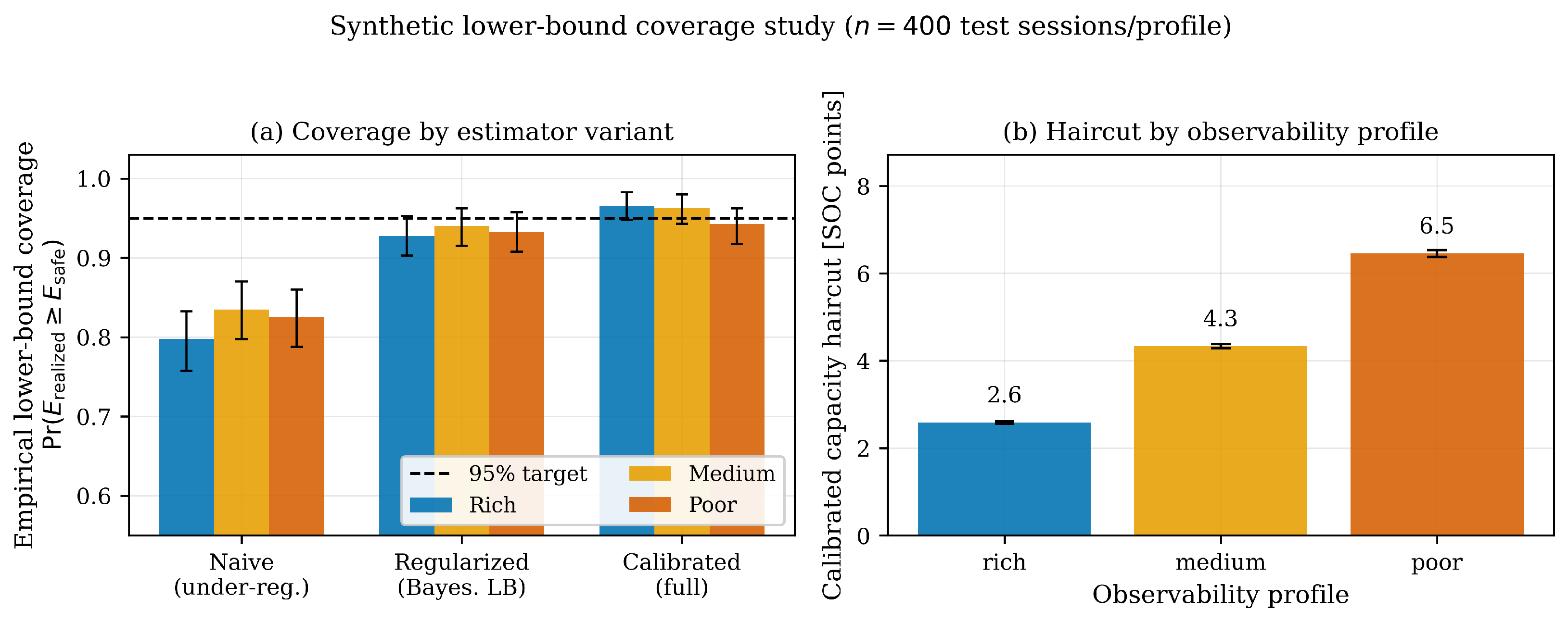
The results are summarized as an ablation in

Table 6. Ablation: lower-bound coverage (95% bootstrap CI) and calibrated haircut, test set ($n=400$ per profile).

Estimator Variant	Rich	Medium	Poor
Point (no UQ)	0.52 [0.47, 0.56]	0.55 [0.50, 0.60]	0.49 [0.44, 0.55]
Naive (under-reg.)	0.80 [0.76, 0.84]	0.83 [0.80, 0.87]	0.82 [0.79, 0.86]
Regularized (Bayes. LB)	0.93 [0.90, 0.95]	0.94 [0.92, 0.96]	0.93 [0.91, 0.95]
Calibrated (conformal)	0.96 [0.95, 0.98]	0.96 [0.94, 0.98]	0.94 [0.92, 0.96]
One-sided 95% lower bound 1	0.946	0.943	0.920
${\kappa }^{★}$ [kWh]	0.38	0.38	0.27
Haircut [SOC pts]	2.6	4.3	6.5

¹ Clopper–Pearson one-sided $95\%$ lower confidence bound on the true coverage of the calibrated bound, from the observed $386/400$, $385/400$ and $377/400$ covered test sessions. This is the quantity to read against the $0.95$ target: a two-sided interval that contains $0.95$ does not establish Equation (6), whereas this bound states what the test set does support. At $n=400$ the bound sits about $0.02$ below the point estimate, so a test set of this size cannot certify $0.95$ empirically even when the conformal construction guarantees it in expectation; the guarantee comes from Equation (15), not from the test frequency.

and Figure 3, with $95\%$ bootstrap confidence intervals (CIs) over the $n=400$ test sessions. A bare point estimate (no uncertainty handling) covers only about $0.5$ (Table 6: $0.49$–$0.55$). A median prediction covers a lower bound at exactly $0.5$ when the realized energy is symmetric about the prediction; the small departures either way reflect slight bias in the noisy point predictor, not a property of the bound. The naive lower quantile, under-regularized with insufficient process and static-parameter uncertainty, covers near $0.82$. Adding process uncertainty and static-parameter regularization yields a Bayesian credible lower bound that raises coverage to $0.93$–$0.94$ but still sits below target in every profile. The full method, which adds the split-conformal margin, reaches $0.94$–$0.96$. Its reliability rests on the finite-sample guarantee of (15) and not on the test frequency: the one-sided lower confidence bounds in Table 6 ($0.946$, $0.943$, $0.920$) show that a 400-session test set cannot by itself certify $0.95$. The calibrated haircut, defined per session as the total conservative margin (point estimate minus deployed calibrated lower bound) normalized to SOC points by that session’s usable capacity and averaged over the test set (A3), grows monotonically as observability degrades, from $2.6$ SOC points (rich) to $4.3$ and $6.5$ SOC points (medium, poor), reproducing deterministically from master seed 20260622 (unrounded $2.58/4.33/6.46$). This quantifies the central trade-off: poorer charger observability is admissible only at the cost of a larger conservative haircut. Because the generator and the estimator share the same forward structure in this experiment, the ablation should be read as a verification that the regularization-and-calibration machinery reaches its nominal target as designed, and that the haircut ordering follows the prescribed prior widths of

Table A1. Generator/estimator prior standard deviations by observability profile.

Profile	${\mathit{\sigma }}_{{\mathit{E}}_{\mathbf{u}}}$ [kWh]	${\mathit{\sigma }}_{{\mathbf{SOC}}_0}$ [pt]	${\mathit{\sigma }}_{\mathit{H}}$	${\mathit{\sigma }}_{\mathbf{aux}}$ [kW]	${\mathit{\sigma }}_{\mathit{b}}$ [kW]
Rich	1.5	1.2	0.008	0.08	0.15
Medium	2.8	2.2	0.016	0.16	0.40
Poor	4.5	3.4	0.030	0.28	0.70

, rather than as an empirical discovery about real charger fleets. The evidence that is not true by construction is the model-mismatch and cross-regime study of Section 5.2, where the generator departs from the estimator’s structure and the calibrated bound is allowed to fail. The same bootstrap procedure underlies the coverage values in the remaining coverage figures (Section 5.2, Section 5.4 and Section 5.6), where the intervals are of comparable width (≈$\pm 0.02$) and are omitted for clarity. All sub-studies (model mismatch, sensitivity, reliability, and baseline comparison) share the seed and configuration of Table 5 and differ only by their stated manipulation; residual coverage differences of about $0.01$–$0.02$ across figures are Monte Carlo and bootstrap variation from the independent per-sub-study random streams rather than method differences.

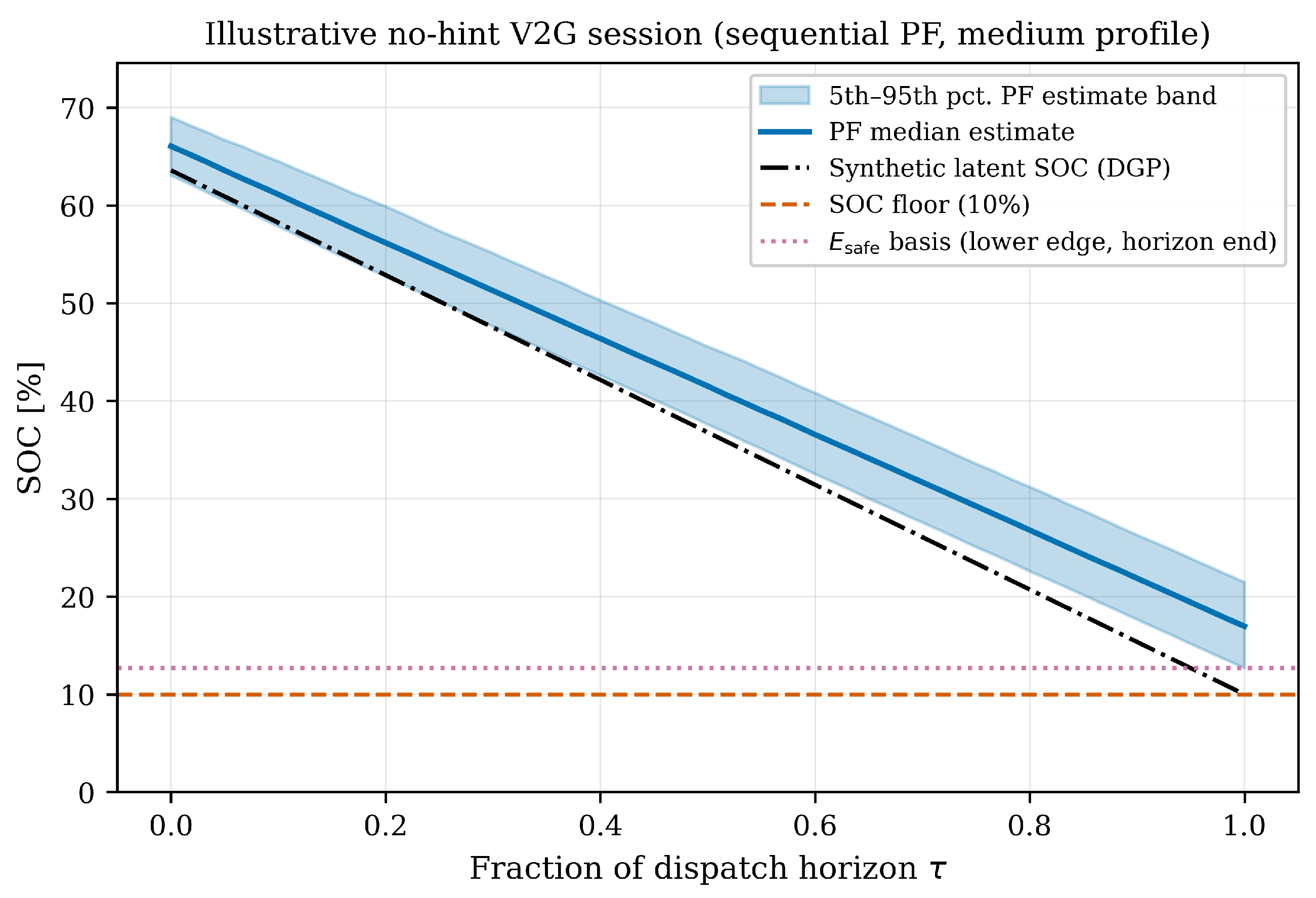
The coverage and haircut numbers above are produced by the conservative-quantile estimator of (13): a static Monte Carlo of the final tradeable-energy expression under jointly sampled uncertain inputs, plus the held-out calibration margin. To confirm that the full sequential filter of Section 4 is not merely specified, it is also run end-to-end on the same synthetic sessions, propagating the augmented state over the discretized dispatch horizon with Liu–West static-parameter moves (and a small metered-power observation noise, without which the delivered-AC-energy state is degenerately hard-capped by metered power times duration) and reading $E_{\mathrm{safe}}$ as the lower quantile of the horizon-end ensemble. With a (non-authoritative) SOC hint injected mid-horizon, the SOC-hint likelihood (12) drives the effective sample size below the $N/2$ threshold and triggers regularized resampling, exercising the assimilation and resampling machinery on data; without a hint the weights are unchanged and no resampling fires, as expected. Run this way, the sequential filter is at least as conservative as the static-quantile estimator on the same sessions (its no-hint lower-bound coverage is not below the corresponding entries of Table 6), so it does not contradict the reported headline numbers. It is not shown to improve them: without a hint the weights are never updated, so the filter is the static estimator, and quantifying what sequential assimilation buys in coverage or haircut on hint-bearing sessions is left to future work; the coverage study is retained as the conservative-quantile evaluation because the filter is a sequential instance of the same lower-quantile-plus-calibration read-out rather than a numerically identical estimator. Figure 4 shows one such filtered session: with no SOC hints, the estimate band widens along the dispatch horizon yet brackets the synthetic latent SOC, and its lower edge stays above the SOC floor, which is the per-session basis for the conservative $E_{\mathrm{safe}}$.

5.2. Model-Mismatch Robustness

A limitation of the matched synthetic setting is that the generator and estimator share the same structure, so coverage validates only the statistical machinery. Robustness is probed with three manipulations: a parameter shift, a structural (functional-form) mismatch, and a broken-exchangeability shift between calibration and test.

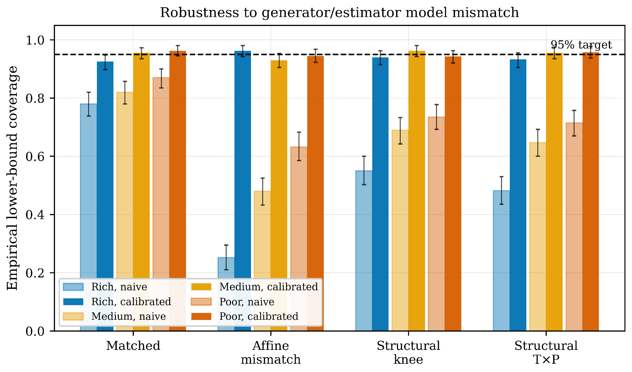
The first is an affine parameter offset: the data generator is given an unmodeled loss term (a temperature-dependent efficiency offset $H_{\mathrm{dis}}\leftarrow H_{\mathrm{dis}}-0.05[1+0.04(20-T)]$, Appendix C) absent from the estimator, so the estimator is systematically over-optimistic about the discharge path. Figure 5 compares the matched and mismatched cases. Under this offset the naive estimator collapses to coverage of $0.30$, $0.50$, and $0.62$ for the rich, medium, and poor profiles—severely over-confident—because its model error is unaccounted for. The calibrated estimator retains near-nominal coverage ($0.95$, $0.95$, $0.95$), close to the matched case ($0.96$, $0.94$, $0.93$). This is the expected behaviour: a near-constant efficiency bias maps to an almost-constant energy shortfall that the held-out margin (14) re-learns, so calibration absorbs it. That test alone is not conclusive: it exercises the one error mode a data-driven additive margin is designed to invert.

To stress the estimator against errors the additive margin cannot trivially invert, two structural mismatches are added that the session-constant estimator cannot represent. The first gives the generator an SOC-dependent efficiency knee, where $H_{\mathrm{dis}}$ drops as the pack discharges through a low-SOC region, so the realized path efficiency depends on how deep each session runs—a shape the estimator’s single effective session-level $H_{\mathrm{dis}}$ cannot capture. The second imposes a multiplicative temperature × power interaction that the estimator’s separable prior omits. Both degrade the naive estimator meaningfully relative to the matched case (naive coverage falling into roughly the $0.55$–$0.73$ and $0.45$–$0.70$ bands across profiles, below the matched $0.78$–$0.87$), confirming a genuine structural error is reaching the estimator; the calibrated estimator still recovers to approximately $0.93$–$0.96$ in both structural cases, i.e., held-out calibration remains effective against structural, not merely affine, model error when calibration and test share the same regime.

The third manipulation deliberately breaks that shared-regime assumption. Calibration sessions are drawn at $T\sim \mathcal{N}(18,8^2)$ °C and the test sessions at a colder $T\sim \mathcal{N}(6,8^2)$ °C, so the calibration and test distributions are no longer exchangeable. Here the calibrated estimator does not fully recover: its coverage settles at approximately $0.92$–$0.95$, below the in-regime $0.94$–$0.96$ band, a modest but measured degradation. This turns the paper’s stated exchangeability caveat into a quantified one. The structural cases mitigate the circularity concern for in-regime operation—calibration is not merely inverting the single error mode it was built for—while the distribution-shift case confirms that coverage need not hold under regime shift, which remains a deployment-time limitation (Section 6.1).

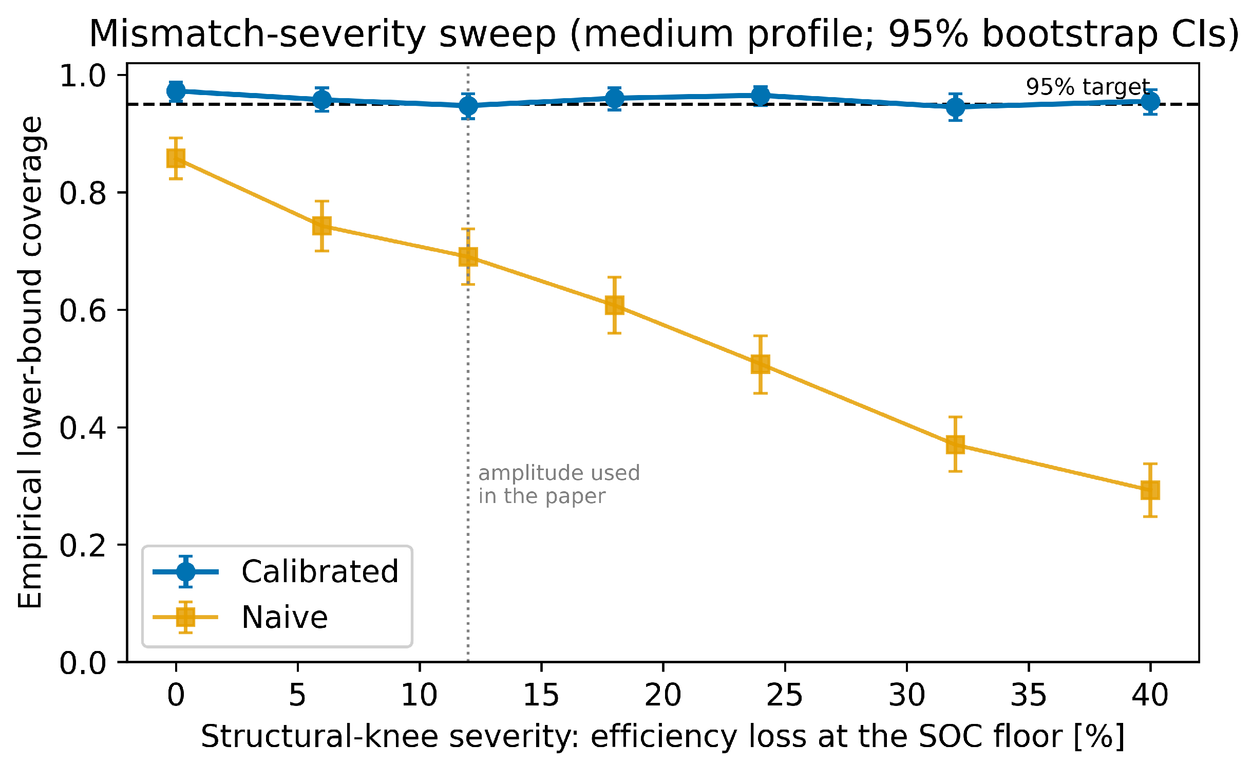
To confirm that the in-regime recovery is not an artifact of the specific mismatch amplitude, Figure 6 sweeps the structural-knee severity from 0 to a $40\%$ efficiency loss at the SOC floor. The naive estimator degrades monotonically (coverage falling from about $0.86$ to $0.28$), whereas the calibrated estimator stays within bootstrap uncertainty of the $95\%$ target across the entire range. The recovery is a general property of the held-out calibration when calibration and test share the regime, not a consequence of the single amplitude used in Figure 5; genuine calibrated failure instead requires the cross-regime distribution shift above.

5.3. Sensitivity of the Conservative Haircut

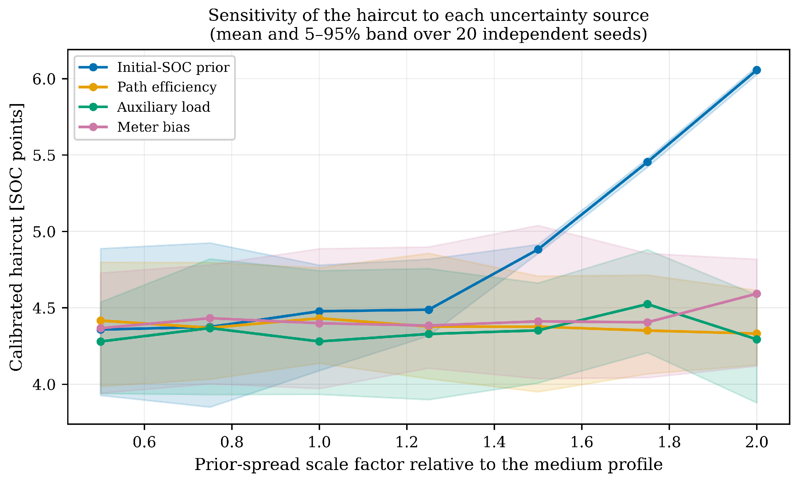
Figure 7 sweeps each uncertainty source independently around the medium profile and reports the resulting calibrated lower-band width. A single run of this sweep is too noisy to rank the sources: the per-point scatter is comparable to the differences between them, and the curves cross. Each point is recomputed over 20 independent seeds and plotted as a mean with a 5–$95\%$ band, so that a ranking is asserted only where the bands separate. Initial-SOC uncertainty is flat up to about $1.25\times$ and then rises steeply, reaching $6.1$ SOC points at $2\times$, with a band narrow enough at the upper end to be clearly separated from every other source. The path-efficiency, auxiliary-load and meter-bias sweeps stay between about $4.3$ and $4.6$ SOC points across the whole range, and their bands overlap each other everywhere, so their apparent ordering is seed noise and no ranking among the three is claimed. The operational conclusion survives the stricter reading: only the initial-SOC prior moves the haircut, which identifies an out-of-pipeline initial-SOC anchor, not finer power metering, as the effective way to reduce it, consistent with the identifiability analysis of Section 3.

5.4. Reliability Across Target Levels

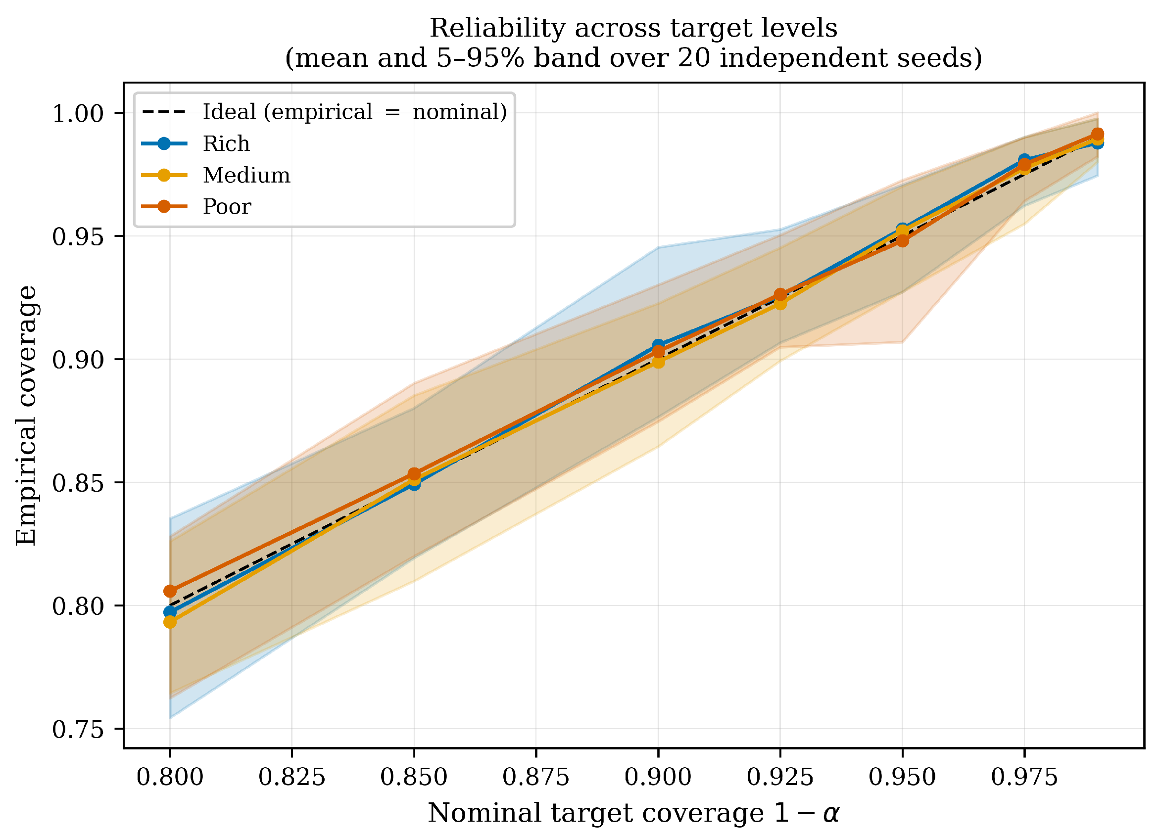
Figure 8 sweeps the nominal target $1-\alpha$ from $0.80$ to $0.99$ and plots the empirical coverage of the calibrated lower bound for all three profiles, again as a mean and 5–$95\%$ band over 20 independent seeds. Because ${\kappa }^{★}$ depends on $\alpha$, the conformal margin is refit on the held-out set at each target level (14). The figure is a consistency check on the margin-selection loop across operating points, not an independent measure of posterior quality: a correctly implemented split-conformal margin drives coverage to the target by construction, so the informative content is whether it does so uniformly and how wide the seed-to-seed spread is. Empirical coverage tracks the diagonal across the whole swept range for all three profiles, with the bands straddling it instead of sitting systematically to one side, and with no visible degradation at either end. The margin is not tuned to a single operating point, so one portfolio can span market products with different reliability requirements: P90 energy products and stricter reserve qualifications are served by the same machinery at different $\alpha$.

5.5. Size of the Calibration Set

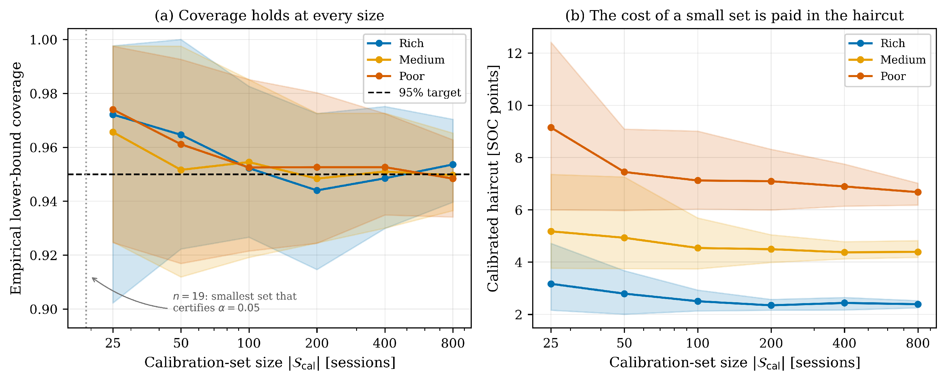
The calibration set has been fixed at 400 sessions per profile throughout. Because that choice governs both the guarantee of Equation (15) and the cost of the margin, Figure 9 and

Table 7. Effect of calibration-set size on coverage and haircut (mean over 20 seeds; fixed 400-session test split).

	Coverage			Haircut [SOC pts]
$\mathbf{|}{\mathcal{S}}_{\mathbf{cal}}\mathbf{|}$	Rich	Med.	Poor	Rich	Med.	Poor
25	0.972	0.966	0.974	3.2	5.2	9.2
50	0.965	0.952	0.961	2.8	4.9	7.5
100	0.952	0.955	0.953	2.5	4.5	7.1
200	0.944	0.948	0.953	2.3	4.5	7.1
400	0.949	0.951	0.953	2.4	4.4	6.9
800	0.954	0.950	0.948	2.4	4.4	6.7

sweep it from 25 to 800 sessions, refitting ${\kappa }^{★}$ at each size and scoring it on a fixed 400-session test split over 20 independent seeds.

The two panels separate cleanly. Coverage is held at every size: the mean sits between $0.944$ and $0.974$ across all profiles and sizes. The lowest cells sit a few thousandths under the nominal $0.95$, within the seed-to-seed spread of it and consistent with the upper bound $1-\alpha +1/(n+1)$ of Equation (15); the guarantee itself holds at every size once $n\ge 19$, and no size shows the systematic under-coverage that a too-small calibration set would produce. A small calibration set costs tradeable capacity, not coverage. At 25 sessions the margin is badly over-conservative, with the haircut reaching $3.2$, $5.2$ and $9.2$ SOC points for the rich, medium and poor profiles; it relaxes as sessions accrue, to $2.4$, $4.4$ and $6.7$ points at 800. The medium and poor profiles relax monotonically; the rich profile is flat past about 200 sessions, where the remaining movement is within the seed spread. The seed-to-seed spread collapses over the same range, from $\pm 2.2$ to $\pm 0.3$ SOC points in the poor profile, so a small set makes the margin larger and unstable.

The 400-session row of Table 7 reports $2.4/4.4/6.9$ SOC points against the $2.6/4.3/6.5$ of Table 6: the former is a mean over 20 seeds, the latter the single canonical run from the master seed. The gap is within the seed-to-seed spread quoted above and is not a change in the result.

Returns diminish past roughly 200 sessions, a usable target for how much history a regime needs before its margin can be trusted; below about 50 the margin is dominated by the tail of the calibration sample and wastes deliverable energy. The cost of a thin calibration set is largest for the regimes that can least afford it: going from 25 to 800 sessions recovers $2.5$ SOC points in the poor profile against $0.8$ in the rich one, because a wider score distribution needs more samples to pin down its upper tail. A poorly observed regime is penalized both by its own telemetry and by the time its margin takes to converge, which strengthens the case for the cold-start fallback of Section 4.4.

5.6. Comparison with Baselines

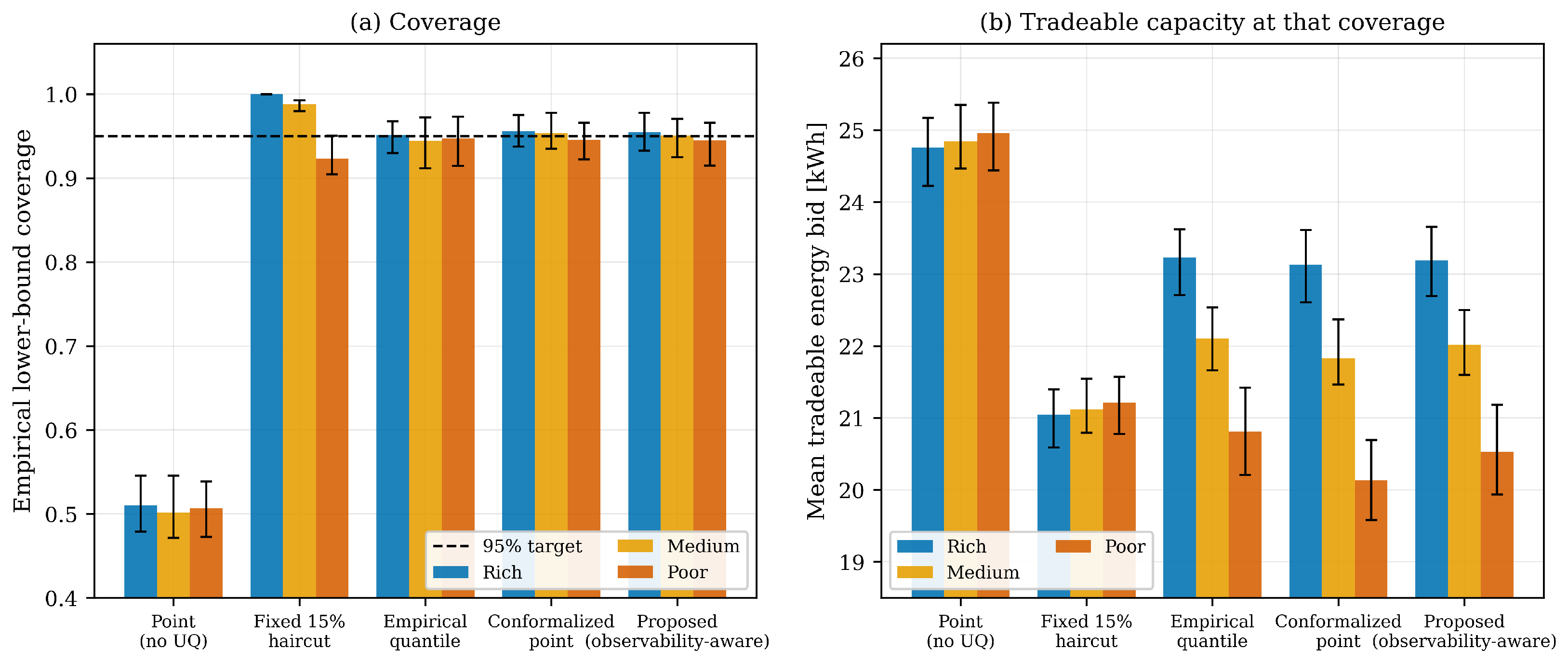
No prior method targets the same per-session observability problem, so the estimator is compared against four alternatives an aggregator could otherwise deploy, spanning two heuristics and two calibrated methods. The point estimate bids the median deliverable energy with no haircut. The fixed-percentage rule bids $85\%$ of that median, a flat $15\%$ reserve. The empirical-quantile baseline is a multiplicative calibration: it scales the point estimate by the $\alpha$-quantile of the realized-to-predicted energy ratio observed on the calibration split. The conformalized-point baseline is the additive counterpart and the strongest comparison available: it applies the same split-conformal margin of Equation (14) to the bare point estimate, with no per-session uncertainty quantification at all. All five are scored on the same sessions over 20 independent seeds, and 

Table 8. Baseline comparison over 20 independent seeds: coverage, mean tradeable energy bid, and abstention rate on the test split.

	Coverage			Tradeable Energy [kWh]
Method	Rich	Med.	Poor	Rich	Med.	Poor
Point (no UQ)	0.510	0.502	0.507	24.76	24.84	24.96
Fixed $15\%$ haircut	1.000	0.988	0.923	21.04	21.12	21.22
Empirical quantile	0.951	0.944	0.947	23.23	22.11	20.81
Conformalized point	0.956	0.954	0.946	23.13	21.83	20.14
Proposed (observ.-aware)	0.955	0.950	0.945	23.19	22.02	20.53

Abstention rate is $0\%$ for every method and profile: the matched generator produces well-posed sessions whose lower quantile never reaches zero, so the abstention path of Table 4 is not exercised by this comparison. Target coverage is $0.95$.

and Figure 10 report coverage, mean tradeable energy, and abstention rate.

The two heuristics fail in the way the observability argument predicts. The point estimate covers about $0.51$, delivering roughly half the time. The fixed $15\%$ haircut is miscalibrated across observability instead of uniformly wrong: it over-covers in the rich and medium profiles ($1.000$ and $0.988$, wasting deliverable flexibility) and under-covers in the poor profile ($0.923$, below target), because one flat percentage cannot track a haircut that has to grow with telemetry quality.

The two calibrated baselines do not fail, which bounds the paper’s claim more tightly than the earlier comparison did. Both reach approximately target coverage in every profile ($0.951/0.944/0.947$ for the empirical quantile, $0.956/0.954/0.946$ for the conformalized point), so coverage is not what distinguishes the proposed estimator. Once any reasonable predictor is conformalized, the coverage statement follows from the calibration step, not from the uncertainty model underneath it. That is a property of conformal prediction, not a finding about V2G: the per-session Monte Carlo is not what makes the bound reliable.

What the per-session ensemble buys is capacity at that reliability, and the size of the gain tracks observability. Against the conformalized point estimate, the proposed estimator bids $23.19$ versus $23.13$ kWh in the rich profile ($+0.3\%$), $22.02$ versus $21.83$ kWh in the medium ($+0.9\%$), and $20.53$ versus $20.14$ kWh in the poor ($+1.9\%$), at coverage that is equal within seed noise. This ordering follows from the construction: a single additive margin must be sized for the worst session in the regime, whereas a session-adaptive bound can be tighter on the sessions whose telemetry happens to be informative, and the room to exploit that grows as sessions become more heterogeneous. The gain is real and consistent in sign, but it is a small single-digit percentage, not an order of magnitude. The multiplicative empirical-quantile rule is competitive on energy, marginally higher than the proposed estimator in all three profiles, while running slightly below target in the medium profile ($0.944$) and carrying no finite-sample guarantee, since a multiplicative rescaling of a point estimate is not a conformal construction; it trades a little coverage for a little energy.

Abstention is zero for every method in this study. The matched generator produces well-posed sessions in which the lower quantile never reaches zero, so the abstention path of Table 4 is not exercised here; it is triggered by the structural conditions of that table and by a margin above the regime ceiling, a case Section 5.5 approaches at the smallest calibration-set sizes in the poor profile. A comparison on well-posed sessions cannot demonstrate abstention, and none is claimed from it.

The comparison narrows what is being claimed. A conformalized point estimate also hits the coverage target, so that is not the contribution. The contribution is that the observability taxonomy determines which sessions can be bid at all, that calibration must be tracked per regime for any of these methods to remain valid, and that the resulting haircut is priced by telemetry quality. The capacity advantage of the per-session ensemble is a secondary benefit that grows as observability degrades.

5.7. Hardware-in-the-Loop AC-Boundary Proof of Concept

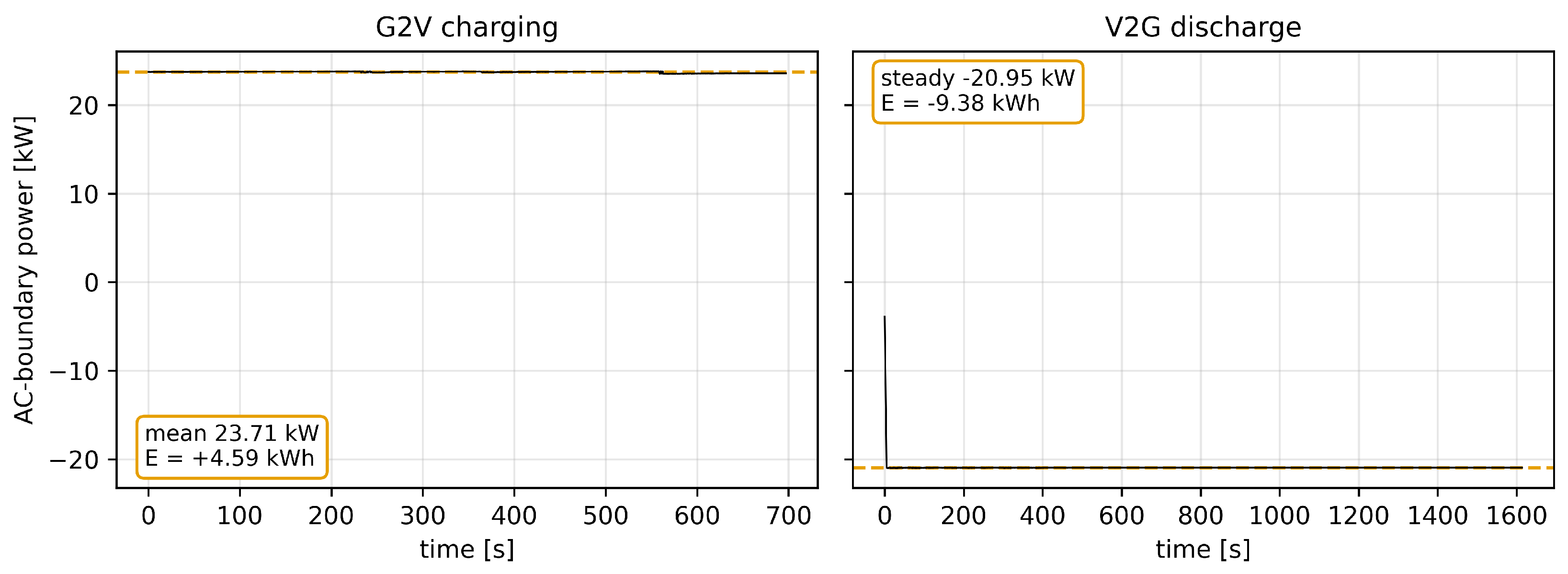
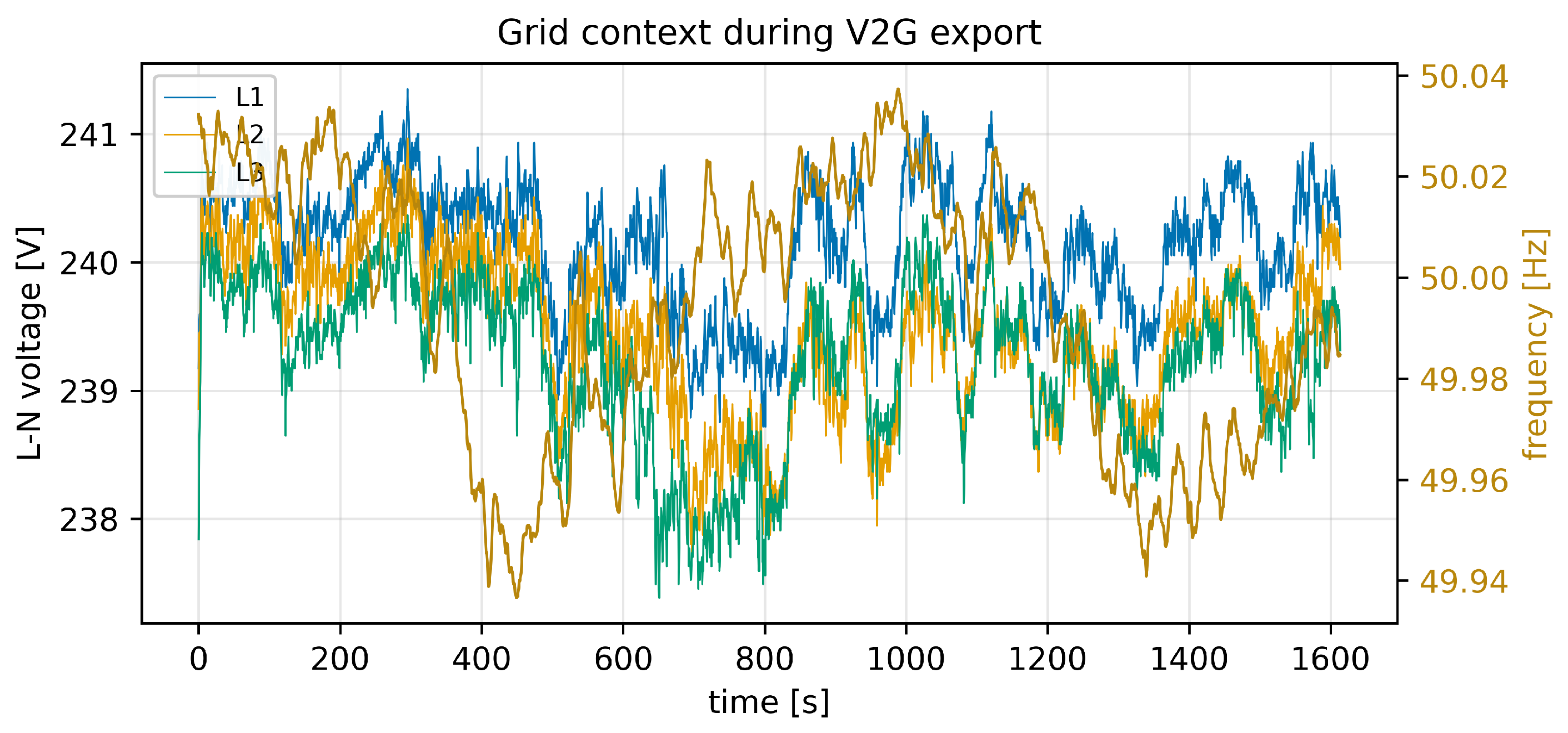
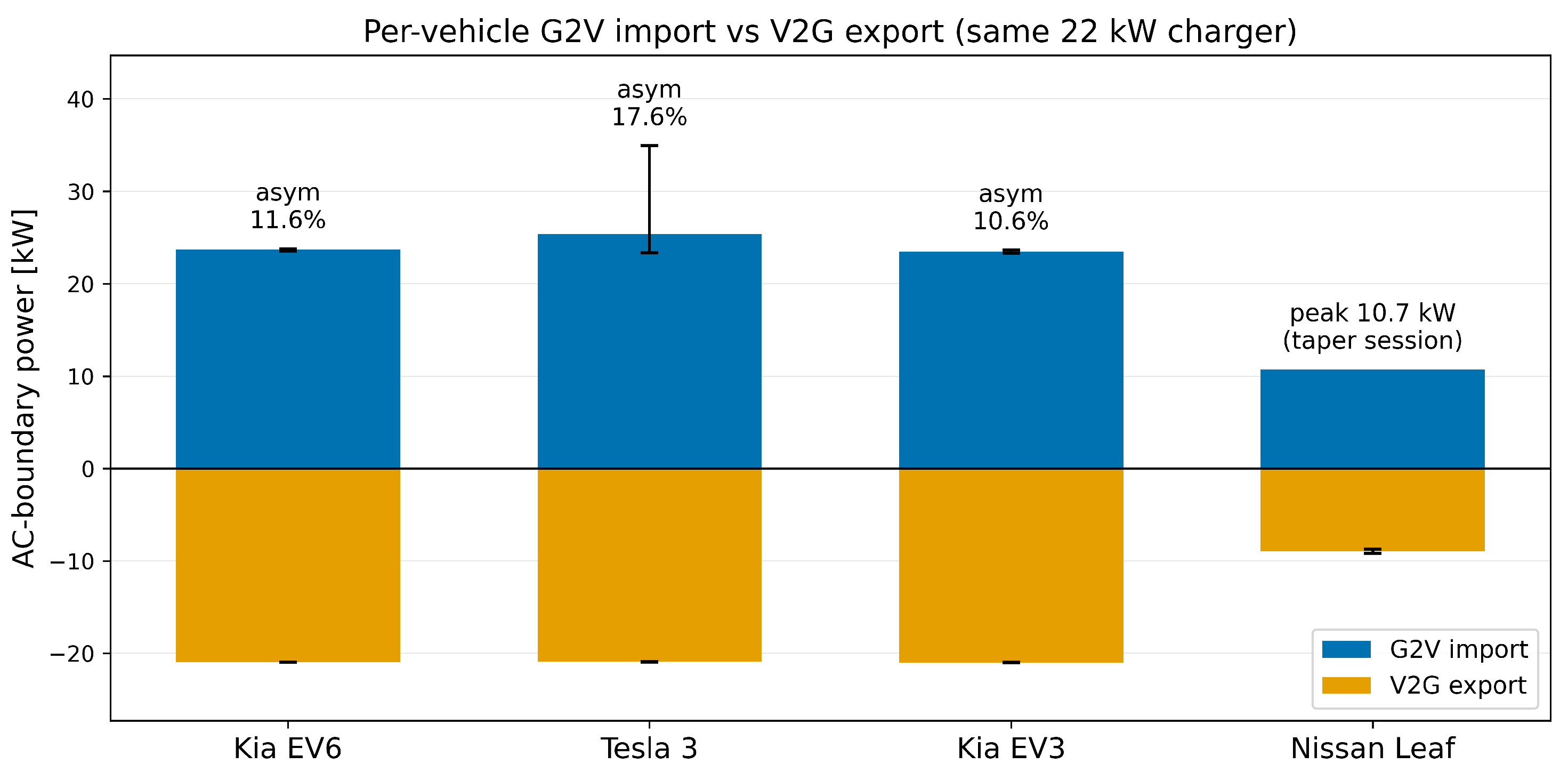
A real Infypower 22 kW bidirectional DC charger using CCS and ISO 15118-20 was connected to a Kia EV6 in the Smart Industry Laboratory and measured at the AC boundary using a PQube power analyzer. The analyzer is a measurement-grade instrument used here as the independent AC-boundary reference; it logged at approximately 2 Hz with 1 s timestamp resolution. Because two samples can share a 1 s timestamp at this rate, energy was integrated on the analyzer’s own uniform sample index (constant nominal sample period) rather than on the rounded wall-clock stamps, so the sub-second ambiguity does not affect the $9.38$ kWh figure; the <1 s cross-stream drift tolerance of the sanity layer applies to alignment between independent streams, which does not arise here since a single stream is integrated. All hardware-in-the-loop quantities in this paper are AC-boundary measurements only; no DC-side meter or vehicle-side anchor was synchronized. The analyzer recorded grid import during grid-to-vehicle (G2V) charging and grid export during V2G discharge. Over the charging window, the measured AC-boundary power was $23.71\pm 0.08$ kW and integrated to 4.59 kWh. Over the V2G discharge window, the measured steady-state AC-boundary export was $-20.95\pm 0.01$ kW and integrated to 9.38 kWh exported. Grid frequency remained within 49.94–50.05 Hz. The absolute power factor was approximately 0.999 in both directions (Figure 11 and Figure 12).

Table 9. PQube AC-boundary hardware-in-the-loop summary.

Metric	G2V	V2G
Window	09:55–10:07	10:09–10:36
Samples	1395	3228
$P_{\mathrm{AC}}$ steady 1	$23.71\pm 0.08$ kW	$-20.95\pm 0.01$ kW
$E_{\mathrm{AC}}$2	$+4.59$ kWh	$-9.38$ kWh
f	49.97–50.05 Hz	49.94–50.04 Hz
$V_{\mathrm{LN}}$ mean	237.0/236.9/235.6 V	240.2/239.5/239.2 V
$\left|PF\right|$	0.999	0.999
Class	B-AC-ref.	B-AC-ref.

¹ Steady-state statistics follow one convention throughout: the G2V import is the mean and standard deviation over the full active window ($P>1$ kW), while the V2G export plateau is the mean and standard deviation over the steady tail (the last $60\%$ of active samples), because the export window contains a ramp that the plateau statistics must exclude. The same convention is used in Table 10. Energies are integrated over the full active window and are therefore unaffected by this choice. ² The G2V and V2G windows are two separately documented operating windows, not a matched charge–discharge cycle; the $+4.59$ and $-9.38$ kWh figures must not be divided to infer efficiency. The $88.4\%$ round-trip efficiency (reported at the end of this section) is computed from separate cumulative-energy metering over a matched charge–discharge cycle at 22 kW.

summarizes the measurement.

The experiment does not validate absolute SOC. It demonstrates ingestion of an independent AC-boundary stream, measurement-topology assignment, power-flow direction from signed physical power, import/export energy integration, and capability classification. In this configuration, the PQube stream provides a measurement reference at the AC boundary, but no DC-side charger meter or battery-side anchor is available; the session is classified as B-AC-reference rather than as a DC diagnostic topology.

The exported PQube metadata field labelled the process step as Idle during sustained physical import/export. The telemetry sanity layer classifies direction and state from signed physical power and energy flow, not from non-authoritative metadata labels; this case shows why.

Campaign-level values documented in separate Smart Industry Laboratory energy and communication summaries reported a round-trip efficiency of 88.4% at 22 kW (computed as the ratio of discharged to charged energy from separate cumulative-energy metering over a matched charge–discharge cycle, and therefore not the ratio of the two window energies in Table 9, which belong to distinct unmatched windows), a session time-to-power-flow of 45.33 s, and a charge-to-discharge transition delay of 13.50 s (both from communication/event logs). These values are included as operating context only; they are not derived from the PQube AC-boundary stream and are not used as estimator validation targets.

5.8. Multi-Vehicle Asymmetry Across a Common Charger

To show that nominal charger rating alone does not determine deliverable V2G capacity, four production EVs were measured at the AC boundary on the same Infypower charger: Kia EV6, Tesla Model 3, and Kia EV3 over CCS2, and a Nissan Leaf over CHAdeMO.

Table 10. Multi-vehicle AC-boundary steady-state summary.

Vehicle	Conn.	G2V [kW]	V2G [kW]	Asym.
Kia EV6	CCS2	$23.7$	$-21.0$	$11.6\%$
Tesla Model 3	CCS2	$25.4$  1	$-20.9$	$17.6\%$
Kia EV3	CCS2	$23.5$	$-21.0$	$10.6\%$
Nissan Leaf	CHAdeMO	$10.7$  2	$-8.9$	—

¹ Median of a broad (wide-spread) profile; see error bars in Figure 13. Only the Tesla Model 3 import is broad (20–35 kW over the active window). ² Measured peak of a partial from-$80\%$-SOC taper, not a steady import; no asymmetry is reported for this vehicle. Convention: G2V is the central value of the full active window (mean, or median where the profile is broad); V2G is the mean of the steady tail (last $60\%$ of active samples), matching Table 9. The Nissan Leaf V2G export is a tight plateau (std $0.205$ kW); all other tabulated values are tight plateaus.

and Figure 13 summarize the steady-state import and export. The V2G export of the three CCS vehicles is nearly identical, between $-20.9$ and $-21.0$ kW, i.e., charger-limited rather than vehicle-limited. In contrast, the G2V import and the resulting import/export asymmetry are vehicle-dependent: the Kia EV3 and EV6 charge near $23.5$–$23.7$ kW with asymmetries of $10.6\%$ and $11.6\%$, whereas the Tesla Model 3 charges over a broad 20–35 kW range (median $25.4$ kW, steady-window tail 21–29 kW) with a larger $17.6\%$ asymmetry, so the median is used as the representative steady import. The 22 kW figure is the charger’s DC-side rating, so the AC-boundary import necessarily exceeds it by the AC/DC conversion loss. Taking the independently metered round-trip efficiency of $88.4\%$ (Section 5.7) and splitting it evenly between the two conversion legs gives ${\eta }_{\mathrm{ch}}=\sqrt{0.884}=0.940$ and an expected AC import at the 22 kW DC rating of $22/0.940=23.4$ kW, within $1.5\%$ of the measured $23.5$–$23.7$ kW. The residual is consistent with the round-trip loss being split unequally between the two legs, which the campaign did not measure. The ratio of the two tabulated window powers is deliberately not used for this: those windows are unmatched (Table 9, footnote 2), and their ratio would equal ${\eta }_{\mathrm{ch}}{\eta }_{\mathrm{dis}}$ only under the additional assumption that the DC-side power was identical in both directions, which was not measured. Steady AC imports of $23.5$–$23.7$ kW are therefore expected rather than anomalous. Read through the same even split they imply $22.1$–$22.3$ kW on the DC side, i.e., the rating within the uncertainty of how the loss divides; only the Tesla’s excursions to 35 kW correspond to DC power clearly above it. The CHAdeMO Nissan Leaf discharged steadily at $-8.9$ kW; its charge was captured only as a partial from-$80\%$-SOC session that tapered from a measured peak of $10.7$ kW down to about $1.4$ kW, so no single steady import represents it and its G2V value is not directly comparable to the other vehicles. It is reported as the measured peak, for completeness rather than as a rated charge power. All sessions held $\left|PF\right|\approx 0.999$.

The Tesla Model 3 does not natively advertise V2G capability, yet the bidirectional charger sustained measured AC-boundary export from it. During discharge the operators also noted that the vehicle dashboard displayed charging while the indicated SOC decreased; this was a real-time operator observation and was not retained as synchronized vehicle-side telemetry, so no claim is made here about the vehicle internal state or protocol-level direction reporting. The retained AC-boundary measurement identifies export unambiguously from signed physical power, consistent with this paper’s premise that direction should be derived from physical measurement rather than from vehicle-reported state [34,35].

These AC-boundary measurements motivate the framework: a single nominal rating or a single efficiency constant cannot represent the deliverable capacity of heterogeneous vehicles, which supports per-session, measurement-based capability assignment and conversion-path uncertainty (Section 3 and Section 4). The measurements characterize the AC boundary and are not used as $E_{\mathrm{safe}}$ deliverability validation or SOC validation.

5.9. Worked Example: Conservative Outputs from Real Telemetry

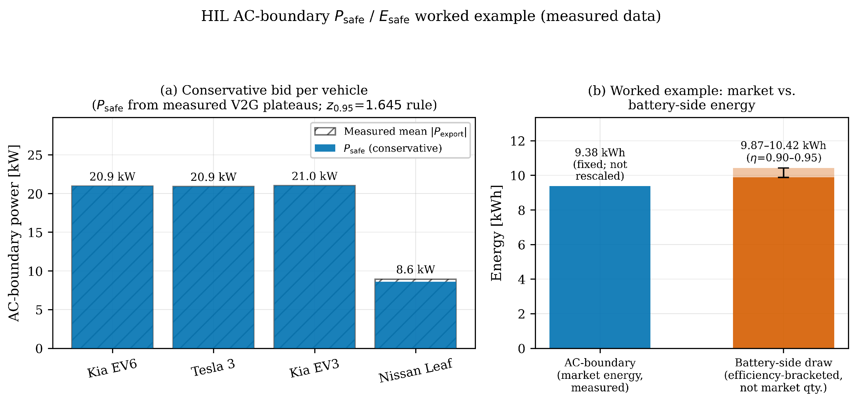
This example illustrates the mapping rule on retained AC-boundary data. It is not a calibrated deliverability validation, and it is not a test of the bound: every quantity below is computed from a completed session, not committed before one. The conservative outputs of Section 4 are applied directly to the Kia EV6 V2G measurement. The steady export plateau is $-20.95$ kW with a measured standard deviation of $0.009$ kW over the steady window; taking the lower quantile of the measured power distribution gives a conservative sustainable power $P_{\mathrm{safe}}\approx 20.95-1.645\left(0.009\right)\approx 20.9$ kW. This hardware-in-the-loop $P_{\mathrm{safe}}$ is a conservative steady-state AC-boundary plateau estimate, not a validated ancillary-service power commitment: ramping, setpoint tracking, command latency, and clipping were not measured because command and DC-side logs were not retained. A full $P_{\mathrm{safe}}$ validation (ramp rate, T50/T90, tracking error) requires the stepped-setpoint experiment noted in Section 6.1. For the energy path, two distinct quantities must be separated, because conservatism runs in opposite directions for each. The market-facing deliverable energy is what can actually be sold at the AC boundary. Here it is the measured throughput itself, $9.38$ kWh, fixed by measurement and not scaled by the discharge efficiency. One point limits what the example can support: $9.38$ kWh is realized throughput, measured after the session ended, and not a pre-dispatch $E_{\mathrm{safe}}$. An $E_{\mathrm{safe}}$ is formed before dispatch from the telemetry available at that moment, and is then either met or missed by what the session goes on to deliver. Nothing of that kind is demonstrated here: the retained windows were not discharges to the declared SOC floor, and no bound was committed in advance of them. What the example shows is the measurement-to-market mapping rule, which boundary each quantity lives at and which direction conservatism runs in, and not the predictive performance of the bound. The experiment that would close this is specified in Section 6. The battery-side draw is a separate quantity: the energy the pack gave up to deliver that AC export, namely $9.38/H_{\mathrm{dis}}$. Applying a literature discharge-path efficiency range of $0.90$–$0.95$ [27,28] brackets the battery-side draw at $9.38/0.95\approx 9.9$ kWh to $9.38/0.90\approx 10.4$ kWh. Being conservative about battery cost (relevant to downstream SOC and energy bookkeeping, not to the market bid) means assuming the pack gave up more per delivered kWh, i.e., the lower path efficiency, which gives the upper bound of $10.4$ kWh on the battery draw. The market-facing $E_{\mathrm{safe}}$ and the battery-side draw are bounded from opposite ends, and neither is obtained by scaling the measured AC energy in the market direction. This demonstrates on real telemetry how an AC-boundary measurement is mapped through the conversion path to an auditable $E_{\mathrm{safe}}/P_{\mathrm{safe}}$—a conservative steady-state plateau estimate under literature efficiency bounds—without any battery-side anchor.

Applying the same lower-quantile rule to all four measured V2G sessions (Figure 14) yields a nonzero conservative bid for every vehicle: $P_{\mathrm{safe}}\approx 20.9$–$21.0$ kW for the three CCS vehicles (only $0.01$–$0.02$ kW below their mean export, because the plateaus are tight), and $P_{\mathrm{safe}}\approx 8.6$ kW for the lower-power Nissan Leaf ($-8.94$ kW mean export, std $0.205$ kW). None of these retained hardware windows triggers abstention. The abstention mechanism of Table 4 is instead exercised on the controlled noisy synthetic sessions of Section 5.1, where telemetry too variable to support a reliable bid drives the lower quantile to zero.

6. Discussion and Conclusions

6.1. Limitations

Four limitations qualify the results. First, the hardware-in-the-loop experiment is scoped as an AC-boundary proof of concept: the campaign did not retain re-processable DC-side charger logs, command/acknowledgement logs, or synchronized battery-side measurements, so it does not close the AC/DC conversion stage online, does not validate DC-side $R_{\mathrm{proxy}}$ or open-circuit-voltage-proxy diagnostics, and does not support quantitative T50/T90 response metrics from the single observed transition. Second, the coverage and haircut figures are established on synthetic sessions; although the model-mismatch study weakens the dependence on a correct generative model—calibration survives structural, not merely affine, mismatch in-regime—the calibrate-versus-test distribution-shift case shows a measured coverage loss when exchangeability breaks, and the end-to-end claim (6) that realized market energy meets the bid is not yet validated against real to-the-limit dispatch. Third, the capability taxonomy and abstention rules are proposed and internally consistent rather than empirically optimized; their thresholds would benefit from tuning on a larger fleet. Fourth, the estimated quantity is energy-limited in the narrow sense defined in Section 4.1: departure uncertainty, requested departure energy, activation duration, ramp rate and setpoint-tracking compliance are outside both the estimator and its validation, so the bound is an observability-limited input to a market offer, not a qualified offer itself. These functions require a dedicated stepped-setpoint experiment with synchronized PQube measurements, charger DC telemetry, command timestamps, and out-of-pipeline vehicle state anchors.

The single most informative next experiment is a pre-dispatch bound test, which the present hardware campaign cannot substitute for. For each session the estimator would be run on the telemetry available at connection time only, and the resulting $E_{\mathrm{safe}}$ committed and logged before any energy is exported. The vehicle would then be discharged to the declared SOC floor instead of being stopped at an arbitrary point, and the realized AC-boundary energy compared against the committed bound. Repeating this over a held-out set of sessions turns the coverage statement (6) into a directly measurable frequency on hardware, which is the one claim this paper establishes in synthesis only. The same runs would supply the stepped-setpoint data needed for the ramp and tracking metrics above, so a single campaign closes both gaps.

6.2. Implications and Future Work

For an aggregator, the practical value of the framework is an upstream decision layer that converts whatever telemetry a charger exposes into a conservative, market-usable capacity and an explicit abstention signal, instead of trusting a single reported SOC value. The capability taxonomy makes the cost of poor observability explicit as a larger capacity haircut, which can inform metering and procurement decisions for charging infrastructure. The sensitivity analysis pinpoints an out-of-pipeline initial-SOC anchor as the most cost-effective observability upgrade. Future work will add synchronized DC-side telemetry and command logging to enable multi-vantage AC/DC stage closure and quantitative response characterization, validate market-deliverability coverage under to-the-limit dispatch, and tune the capability thresholds on a larger multi-charger fleet.

6.3. Conclusions

This paper presented an observability-aware framework for converting heterogeneous charger telemetry into conservative tradeable V2G capacity. The framework distinguishes measurement references from state anchors, models measurement-to-battery conversion paths, treats vehicle-reported SOC and capacity as non-authoritative hints, and abstains when observability or calibration is insufficient. The synthetic study shows the need for regularization and held-out coverage calibration and quantifies the observability-dependent haircut. The model-mismatch, sensitivity, calibration-size and reliability studies quantify, under controlled in-regime conditions, how regularization and split-conformal calibration move the bound to the target, and identify initial-SOC uncertainty as the dominant driver of the conservative haircut; they do not establish coverage under arbitrary deployment shift. The baseline comparison bounds the claim: once any reasonable predictor is conformalized it reaches the coverage target, so reliability follows from the calibration step and not from the per-session uncertainty model, and what the observability-aware ensemble adds is tradeable capacity at that reliability, a single-digit percentage that grows as telemetry degrades. Two caveats belong with any use of these results. The coverage guarantee is the marginal, finite-sample conformal statement of Equation (15), conditional on exchangeability within a capability regime; it is not a per-session guarantee and does not survive shift across regimes, so calibration must be maintained per regime and refreshed as fleets and firmware change. A regime also cannot certify a margin until it has accrued enough completed sessions, with the smallest usable set well above the formal minimum of 19 at $\alpha =0.05$. The hardware-in-the-loop proof of concept demonstrates AC-boundary telemetry ingestion and capability assignment on real bidirectional charging hardware. It does not validate end-to-end deliverability under market dispatch: every hardware quantity reported here is realized throughput measured after a session ended, whereas a market bound must be committed before one begins and then met. The coverage claim (6) is established in synthesis only, and the pre-dispatch discharge-to-floor experiment specified in Section 6.1 is what would close it on hardware. Campaign AC-boundary measurements on four vehicles indicate that V2G export can be charger-limited while import and asymmetry are vehicle-dependent, which supports per-session over single-rating capability assignment; these measurements are reported as operating context rather than as deliverability validation.

References

1. Ru, J.; Gillott, M.; Shipman, R. Vehicle-to-Grid (V2G) Research: A Decade of Progress, Achievements, and Future Directions. Energies 2025, 18, 6148. [Google Scholar] [CrossRef] [Scilit]
2. Jokinen, I.; Lehtonen, M. Flexibility of Electric Vehicle Charging with Demand Response and Vehicle-to-Grid for Power System Benefit. IEEE Access 2024, 12, 129594–129609. [Google Scholar] [CrossRef] [Scilit]
3. Wang, Q.; Huang, C.; Wang, C.; Li, K.; Shafie-khah, M. Risk-Averse Frequency Regulation Strategy of Electric Vehicle Aggregator Considering Multiple Uncertainties. Appl. Energy 2025, 382, 125259. [Google Scholar] [CrossRef] [Scilit]
4. Najar, A.; Yang, H.; Ye, J.; Song, W. A Data-Driven Algorithm for Estimating Battery State of Charge via Smart Plug-Based PCC Measurements. In Proceedings of the IEEE Applied Power Electronics Conference and Exposition (APEC), San Antonio, TX, USA, 22–26 March 2026. [Google Scholar] [CrossRef] [Scilit]
5. Pasetti, M.; Dello Iacono, S.; Zaninelli, D. Real-Time State of Charge Estimation of Light Electric Vehicles Based on Active Power Consumption. IEEE Access 2023, 11, 111304–111319. [Google Scholar] [CrossRef] [Scilit]
6. Zakharov, A.; Volovich, V.; Makarov, I. Transferable Electric Vehicle Battery Capacity Estimation from Real-World Charging Data Using Spectral Learning. IEEE Open J. Ind. Electron. Soc. 2026, 7, 892–904. [Google Scholar] [CrossRef] [Scilit]
7. Arulampalam, M.S.; Maskell, S.; Gordon, N.; Clapp, T. A Tutorial on Particle Filters for Online Nonlinear/Non-Gaussian Bayesian Tracking. IEEE Trans. Signal Process. 2002, 50, 174–188. [Google Scholar] [CrossRef] [Scilit]
8. Fan, Y.; Chi, Q.; Fang, X.; Tian, J.; Li, M.; Liu, X. State-of-Charge Estimation of Lithium-Ion Batteries Using an Adaptive Particle Filter Based on an Improved Particle Swarm Optimization Algorithm. IEEE Trans. Transp. Electrif. 2025, 11, 9428–9440. [Google Scholar] [CrossRef] [Scilit]
9. Jiao, Z.; Gao, Z.; Chai, H. Estimating State of Charge of Lithium-Ion Battery Using an Adaptive Fractional-Order Kalman–Unscented Particle Filter. J. Energy Storage 2025, 131, 116873. [Google Scholar] [CrossRef] [Scilit]
10. Chen, Y.; Li, R.; Sun, Z.; Zhao, L.; Guo, X. SOC Estimation of Retired Lithium-Ion Batteries for Electric Vehicle with Improved Particle Filter by H-Infinity Filter. Energy Rep. 2023, 9, 1937–1947. [Google Scholar] [CrossRef] [Scilit]
11. Ahwiadi, M.; Wang, W. An Enhanced Particle Filter Technology for Battery System State Estimation and RUL Prediction. Measurement 2022, 191, 110817. [Google Scholar] [CrossRef] [Scilit]
12. Lee, Z.J.; Lee, G.; Lee, T.; Jin, C.; Lee, R.; Low, Z.; Chang, D.; Ortega, C.; Low, S.H. Adaptive Charging Networks: A Framework for Smart Electric Vehicle Charging. IEEE Trans. Smart Grid 2021, 12, 4339–4350. [Google Scholar] [CrossRef] [Scilit]
13. Pertl, M.G.; Carducci, F.; Tabone, M.; Marinelli, M.; Kiliccote, S.; Kara, E.C. An Equivalent Time-Variant Storage Model to Harness EV Flexibility: Forecast and Aggregation. IEEE Trans. Ind. Inform. 2019, 15, 1899–1910. [Google Scholar] [CrossRef] [Scilit]
14. Genov, E.; De Cauwer, C.; Van Kriekinge, G.; Coosemans, T.; Messagie, M. Forecasting Flexibility of Charging of Electric Vehicles: Tree and Cluster-Based Methods. Appl. Energy 2024, 353, 121969. [Google Scholar] [CrossRef] [Scilit]
15. Ko, K.; Lee, E.; Baek, K. Techno-Probabilistic Flexibility Assessment of EV2G Based on Chargers’ Historical Records. Energies 2025, 18, 2031. [Google Scholar] [CrossRef] [Scilit]
16. Schlund, J.; Pruckner, M.; German, R. FlexAbility—Modeling and Maximizing the Bidirectional Flexibility Availability of Unidirectional Charging of Large Pools of Electric Vehicles. In Proceedings of the Eleventh ACM International Conference on Future Energy Systems (e-Energy), Online, 22–26 June 2020; pp. 121–132. [Google Scholar] [CrossRef] [Scilit]
17. Zhou, M.; Wu, Z.; Wang, J.; Li, G. Forming Dispatchable Region of Electric Vehicle Aggregation in Microgrid Bidding. IEEE Trans. Ind. Inform. 2021, 17, 4755–4765. [Google Scholar] [CrossRef] [Scilit]
18. Li, Y.; Li, Z. Distributionally Robust Evaluation for Real-Time Flexibility of Electric Vehicles Considering Uncertain Departure Behavior and State-of-Charge. IEEE Trans. Smart Grid 2024, 15, 4288–4291. [Google Scholar] [CrossRef] [Scilit]
19. Ke, S.; Zhang, K.; Mai, W.; Guo, R.; He, S.; Tian, J.; Chung, C.Y. Maximizing Intraday V2G Feasible Capacity of EVs: A Cross-Disciplinary Approach with Traffic Flow and Prospect Theory. IEEE Trans. Transp. Electrif. 2026, 12, 5078–5091. [Google Scholar] [CrossRef] [Scilit]
20. Mukhi, K.; Qu, C.; You, P.; Abate, A. Robust Aggregation of Electric Vehicle Flexibility. In Proceedings of the 28th ACM International Conference on Hybrid Systems: Computation and Control (HSCC), Irvine, CA, USA, 6–9 May 2025. [Google Scholar] [CrossRef] [Scilit]
21. García-Cerezo, A.; Bonilla, D.; Baringo, L.; García-González, J. A Stochastic Adaptive Robust Optimization Approach to Build Day-Ahead Bidding Curves for an EV Aggregator. IEEE Trans. Ind. Appl. 2026, 62, 244–255. [Google Scholar] [CrossRef] [Scilit]
22. Pipada Sunil Kumar, Y.; Pourmousavi, S.A.; Liisberg, J.A.R.; Lesmos-Vinasco, J. Calibrated Uncertainty Quantification for Prosumer Flexibility Aggregation in Ancillary Service Markets. arXiv 2026, arXiv:2601.14663. [Google Scholar]
23. Angelopoulos, A.N.; Bates, S. Conformal Prediction: A Gentle Introduction. Found. Trends Mach. Learn. 2023, 16, 494–591. [Google Scholar] [CrossRef] [Scilit]
24. Romano, Y.; Patterson, E.; Candès, E.J. Conformalized Quantile Regression. In Proceedings of the Neural Information Processing Systems (NeurIPS), Vancouver, BC, Canada, 8–14 December 2019; pp. 3543–3553. [Google Scholar]
25. O’Connor, C.; Bahloul, M.; Rossi, R.; Prestwich, S.; Visentin, A. Conformal Prediction for Electricity Price Forecasting in the Day-Ahead and Real-Time Balancing Market. Energy AI 2025, 21, 100571. [Google Scholar] [CrossRef] [Scilit]
26. Nam, N.B.; Ogliari, E.; Leva, S.; Pafumi, E.; Alberti, D.; Duong, M.Q. Comparative Analysis of Conformal Prediction Techniques and Machine Learning Models for Very Short-Term Solar Power Forecasting. Energy AI 2025, 21, 100573. [Google Scholar] [CrossRef] [Scilit]
27. Apostolaki-Iosifidou, E.; Codani, P.; Kempton, W. Measurement of Power Loss during Electric Vehicle Charging and Discharging. Energy 2017, 127, 730–742. [Google Scholar] [CrossRef] [Scilit]
28. Schram, W.; Brinkel, N.; Smink, G.; van Wijk, T.; van Sark, W. Empirical Evaluation of V2G Round-Trip Efficiency. In Proceedings of the International Conference on Smart Energy Systems and Technologies (SEST), Online, 7–9 September 2020. [Google Scholar] [CrossRef] [Scilit]
29. Zecchino, A.; Thingvad, A.; Andersen, P.B.; Marinelli, M. Test and Modelling of Commercial V2G CHAdeMO Chargers to Assess the Suitability for Grid Services. World Electr. Veh. J. 2019, 10, 21. [Google Scholar] [CrossRef] [Scilit]
30. Pedersen, K.L.; Knudsen, R.M.; Marinelli, M.; Secchi, M.; Sevdari, K. Enabling Grid Services with Bidirectional EV Chargers: A Comparative Analysis of CCS2 and CHAdeMO Response Dynamics. World Electr. Veh. J. 2025, 16, 636. [Google Scholar] [CrossRef] [Scilit]
31. Neaimeh, M.; Andersen, P.B. Mind the Gap—Open Communication Protocols for Vehicle Grid Integration. Energy Inform. 2020, 3, 1. [Google Scholar] [CrossRef] [Scilit]
32. Uribe-Pérez, N.; Gonzalez-Garrido, A.; Gallarreta, A.; Justel, D.; González-Pérez, M.; González-Ramos, J.; Arrizabalaga, A.; Asensio, F.J.; Bidaguren, P. Communications and Data Science for the Success of Vehicle-to-Grid Technologies: Current State and Future Trends. Electronics 2024, 13, 1940. [Google Scholar] [CrossRef] [Scilit]
33. van der Kam, M.; Bekkers, R. Mobility in the Smart Grid: Roaming Protocols for EV Charging. IEEE Trans. Smart Grid 2023, 14, 810–822. [Google Scholar] [CrossRef] [Scilit]
34. Rahman, A.B.; Siraj, M.S.; Tsiropoulou, E.E.; Fragkos, G.; Sullivant, R.; Choe, Y.R.; Rhee, J.; Lee, K.H. Reevaluating Optional Fields in OCPP 2.0.1: Preliminary Case Study by Spoofing State of Charge. In Proceedings of the IEEE International Workshop on Computer Aided Modeling and Design of Communication Links and Networks (CAMAD), Tempe, AZ, USA, 14–16 October 2025. [Google Scholar] [CrossRef] [Scilit]
35. Heinekamp, J.F.; Mendy, R.C.; Smitmans, L.; Strunz, K. Realizing Smart Charging of Electric Vehicles at Public Charging Infrastructures Using Standards-Based Communication Architecture. In Proceedings of the IEEE International Conference on Communications, Control, and Computing Technologies for Smart Grids (SmartGridComm), Oslo, Norway, 17–20 September 2024. [Google Scholar] [CrossRef] [Scilit]
36. Open Charge Alliance. Open Charge Point Protocol 2.0.1. Also Published as IEC 63584:2024, 2020. Available online: https://openchargealliance.org (accessed on 28 July 2026).
37. ISO Standard 15118-20:2022; Road Vehicles—Vehicle to Grid Communication Interface—Part 20: 2nd Generation Network and Application Protocol Requirements. International Organization for Standardization: Geneva, Switzerland, 2022.
38. Mądziel, M.; Campisi, T. Predicting Auxiliary Energy Demand in Electric Vehicles Using Physics-Based and Machine Learning Models. Energies 2025, 18, 6092. [Google Scholar] [CrossRef] [Scilit]
39. Bellman, R.; Åström, K.J. On Structural Identifiability. Math. Biosci. 1970, 7, 329–339. [Google Scholar] [CrossRef] [Scilit]
40. Toubeau, J.F.; Bottieau, J.; De Grève, Z.; Vallée, F.; Bruninx, K. Data-Driven Scheduling of Energy Storage in Day-Ahead Energy and Reserve Markets with Probabilistic Guarantees on Real-Time Delivery. IEEE Trans. Power Syst. 2021, 36, 2815–2828. [Google Scholar] [CrossRef] [Scilit]
41. Gordon, N.J.; Salmond, D.J.; Smith, A.F.M. Novel Approach to Nonlinear/Non-Gaussian Bayesian State Estimation. IEE Proc. F (Radar Signal Process.) 1993, 140, 107–113. [Google Scholar] [CrossRef] [Scilit]
42. Liu, J.; West, M. Combined Parameter and State Estimation in Simulation-Based Filtering. In Sequential Monte Carlo Methods in Practice; Springer: New York, NY, USA, 2001; pp. 197–223. [Google Scholar] [CrossRef] [Scilit]
43. Musso, C.; Oudjane, N.; Le Gland, F. Improving Regularised Particle Filters. In Sequential Monte Carlo Methods in Practice; Doucet, A., de Freitas, N., Gordon, N., Eds.; Springer: New York, NY, USA, 2001; pp. 247–271. [Google Scholar] [CrossRef] [Scilit]
44. Tibshirani, R.J.; Foygel Barber, R.; Candès, E.J.; Ramdas, A. Conformal Prediction under Covariate Shift. In Proceedings of the Neural Information Processing Systems (NeurIPS), Vancouver, BC, Canada, 8–14 December 2019; Volume 32. [Google Scholar]
45. Gibbs, I.; Candès, E.J. Adaptive Conformal Inference under Distribution Shift. In Proceedings of the Neural Information Processing Systems (NeurIPS), Online, 6–14 December 2021; Volume 34. [Google Scholar]
Figure 1. Observability-aware safe-capacity pipeline. Sessions failing sanity, observability, or calibration checks are routed to abstention.
Applsci 16 09410 g001
Figure 2. Measurement-to-battery conversion path for a DC charger. An AC-boundary meter observes the full path (class B-AC); a DC-output meter shortens the unobserved path (class A-DC).
Applsci 16 09410 g002
Figure 3. Synthetic lower-bound coverage study (Monte Carlo of Table 5; generator and calibration fully specified in Appendix C). (a) Empirical lower-bound coverage with 95 % bootstrap confidence intervals for the naive (under-regularized), regularized (Bayesian credible lower bound), and calibrated (full) estimators against the 95 % target. (b) Calibrated lower-band width (capacity haircut) in SOC points by observability profile (error bars are 95 % bootstrap CIs). Market deliverability coverage, Pr ( E realized ≥ E safe ) ≥ 1 − α , is a separate hardware-in-the-loop objective when to-the-limit dispatch is available.
Applsci 16 09410 g003
Figure 4. Illustrative no-hint V2G session, selected among candidates whose lower band clears the SOC floor by a visible margin; under the fully-depleting generative model most sessions clear the floor only marginally, so this trajectory is a favourable rather than typical case. The 5–95% estimate band brackets the synthetic latent SOC and widens over the horizon; the conservative bound is read from the lower edge.
Applsci 16 09410 g004
Figure 5. Robustness to generator/estimator model mismatch (bars are point coverage; error bars are 95 % bootstrap CIs over the n = 400 test sessions). The naive estimator becomes severely over-confident when its efficiency model is wrong, whereas held-out calibration keeps the lower bound near the 95% target.
Applsci 16 09410 g005
Figure 6. Mismatch-severity sweep (medium profile; 95 % bootstrap CIs). As the structural-knee efficiency loss at the SOC floor grows, the naive estimator degrades monotonically while the calibrated estimator holds near the 95 % target across the full range, so the in-regime recovery is not specific to the amplitude used elsewhere.
Applsci 16 09410 g006
Figure 7. Sensitivity of the calibrated haircut to each uncertainty source, as the mean and 5– 95 % band over 20 independent seeds. Only the initial-SOC prior moves the haircut, and only above about 1.25 × ; the efficiency, auxiliary-load and meter-bias bands overlap throughout, so they are not separable from one another.
Applsci 16 09410 g007
Figure 8. Reliability of the calibrated lower bound: empirical versus nominal target coverage across observability profiles, as the mean and 5– 95 % band over 20 independent seeds. Coverage tracks the diagonal across the swept range in all three profiles.
Applsci 16 09410 g008
Figure 9. Effect of calibration-set size, as the mean and 5– 95 % band over 20 independent seeds. (a) Coverage is held at every size, including the smallest set that certifies α = 0.05 . (b) The cost of a small calibration set is paid entirely in the haircut, and falls hardest on the poorly observed profile.
Applsci 16 09410 g009
Figure 10. Baseline comparison over 20 independent seeds. (a) A point estimate is over-confident and a fixed-percentage haircut is miscalibrated across observability regimes, while all three calibrated methods track the 95 % target. (b) At that matched coverage the methods differ in how much capacity they leave tradeable; the proposed estimator’s advantage over a conformalized point estimate grows as observability degrades.
Applsci 16 09410 g010
Figure 11. AC-boundary power measured by the PQube analyzer during real G2V charging and V2G discharge of a Kia EV6 connected to an Infypower 22 kW bidirectional CCS charger. Positive power denotes grid import; negative power denotes export.
Applsci 16 09410 g011
Figure 12. Phase-to-neutral voltages and grid frequency recorded at the AC boundary during V2G export. The trace provides grid-side context, not a battery-state anchor.
Applsci 16 09410 g012
Figure 13. Per-vehicle steady-state G2V import and V2G export at the AC boundary on the same 22 kW bidirectional charger. Error bars span the 10th–90th percentile over the same window as the tabulated value: the full active window for G2V, the steady tail for V2G. The Nissan Leaf G2V bar is a measured peak of a taper session, so no percentile band applies to it. V2G export is charger-limited across the CCS vehicles; import and asymmetry are vehicle-dependent.
Applsci 16 09410 g013
Figure 14. Conservative deliverable power P safe from the measured V2G plateaus. All four sessions are tight enough to yield a nonzero conservative bid: the CCS plateaus give P safe close to their mean export (≈ 20.9 – 21.0 kW), and the CHAdeMO Nissan Leaf export ( − 8.94 kW, std 0.205 kW) gives P safe ≈ 8.6 kW. Panel (b) shows the energy mapping: measured AC market energy (fixed) versus the efficiency-bracketed battery-side draw.
Applsci 16 09410 g014