A Hybrid Calculation Method for Determining the Frequency Characteristics of the Air-Cored Coils with Complex Structure

Abstract

Hollow coils with complex structures are very common in electrical equipment and sensors. Additionally, the responses at different frequencies are an important characteristic of the coils. However, it is quite challenging to divide the irregular coils with fine windings (thousands of turns and wire diameter less than 0.2 mm) into meshes using finite element simulation software (FESS), much less perform the simulation calculations, as theoretical derivations are only applicable to coils with specific shapes. This issue presents challenges in designing coils with high-density, multi-turn and irregular structures. Thus, we propose a calculation method for determining the frequency characteristics of hollow coils with such structures. To validate this method, three sets of hollow coils with complex structures and high-density winding were fabricated. These coils included two coupled PCB coils, one coil with thousands of fine turns, and a PCB coil with a complex and were tested using an LCR analyzer with a frequency range of 0 to 2 MHz. The experimental results showed good agreement with numerical calculations.

1. Introduction

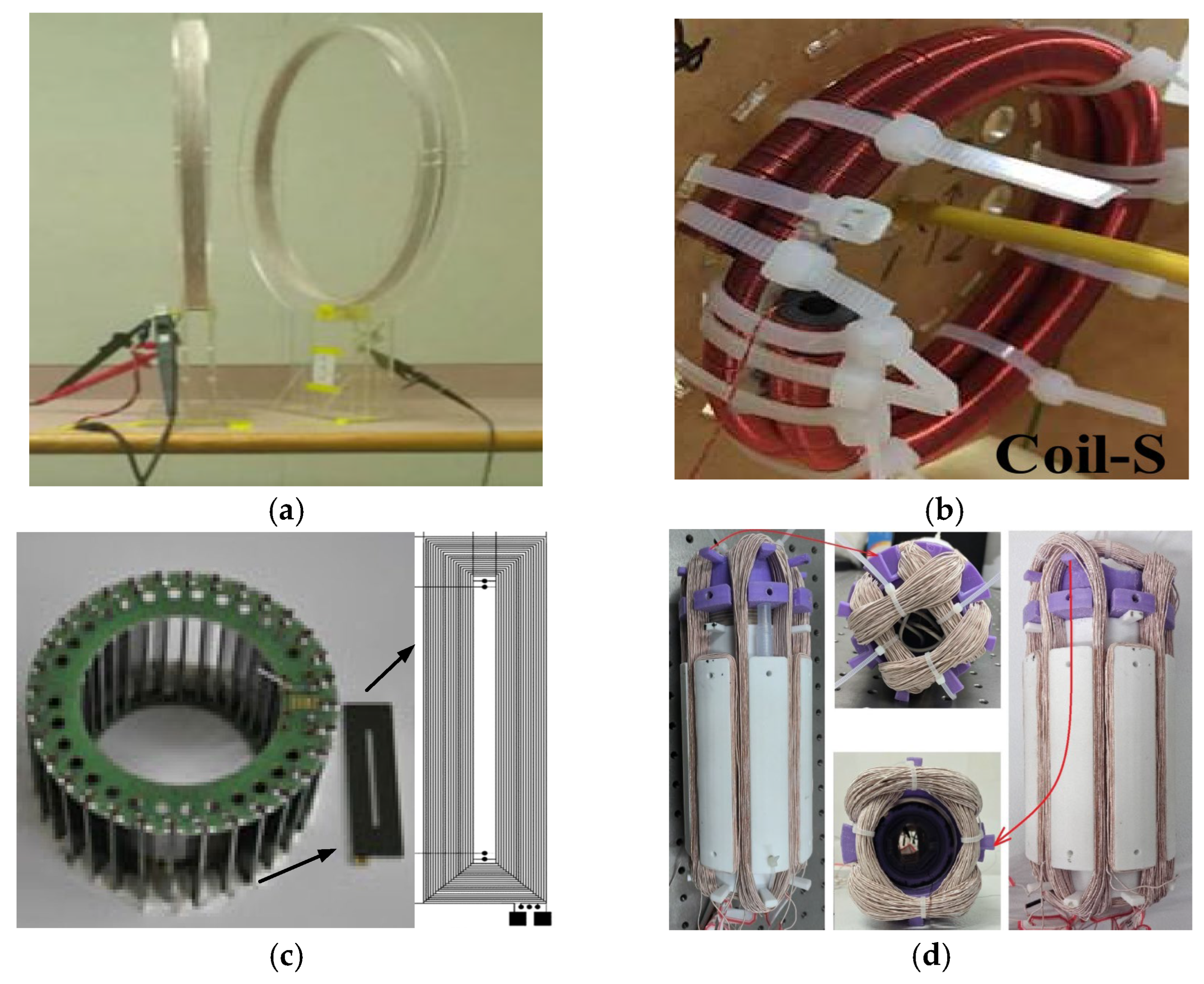
As a common electrical component, the air-cored coils play a variety of important roles in electrical equipment and motors [1,2,3], such as blocking alternating current (AC) [4], measuring magnetic fields [5,6,7], detecting metal [8], electromagnetic tomography [9], detecting cardiac magnetic signals [10], electromagnetic thermotherapy [11], performing precise quantum measurements [12], Moving RFID Microtag Detection [13], measuring currents [14,15,16], crack detection [17], generating desired magnetic environments (Holmholly coils) [18,19], forming inductive power transfer (IPT) energy transmission systems [20,21]. Figure 1 shows three types of air-cored coils.

The frequency characteristics of the air-cored coil influence electrical equipment performance [22], and the impedance changes in the coil are often used to determine the dimensions and state of the object being detected [23,24]. The frequency characteristics are affected by parasitic inductance, parasitic capacitance, and skin-effect resistance. Thus, these parameters must be calculated precisely before designing the coil and circuit. Therefore, methods for calculating the frequency characteristics and coil parameters have been studied by many researchers. Three methods are used to determine the frequency characteristics of coil ports.

The first is the numerical calculation method based on theoretical derivation. In this method, the spiral turns of a regular-shaped coil are often equivalent to rings and include methods for calculating the mutual and self-inductance of two-plane spiral coils [25], the impedance of a cylindrical coil for detecting eddy current displacements [26], the mutual inductance of two coaxial and non-coaxial planar spiral windings [27]. Another numerical calculation method is exclusively used for coils with regular structures and evenly distributed turns [28], which include planar spiral coils and linear tubular coils [29,30]. The second coil type is used in electromagnetic simulation software to conduct three-dimensional simulations of coils with a small number of turns [31]. For example, the electrical parameters of a three-turn coil are calculated using FESS [32]. The mutual and self-inductances between two eight-turn coils with thicker windings were obtained via the Q3D software in [33]. The last method involves the use of an instrument to measure the impedance and coil frequency characteristics. Specifically, a method for measuring the mutual inductance of a superconducting coil based on the standard square wave compensation method was proposed to measure Planck’s constant more accurately [34]. The author of [35] provided a method to estimate the insulation deterioration characteristics under different failure mechanisms by measuring the variation in coil impedance. The model-derived parameters of the coils are obtained by applying nonlinear regression to the experimental data provided by an impedance analyzer [36].

From the above, it can be seen that the current methods for calculating coil parameters are not applicable to coils with irregular structures and fine winding (hundreds or thousands of turns with wire diameters less than 0.1 mm). From a theoretical derivation perspective, these coils usually comprise a series of regular ring structures or a metal tube. However, when the coil does not have a regular ring structure and a metal tube, this method will fail, as shown in Figure 1c. Moreover, mesh division calculations cannot be easily performed with commonly used electromagnetic simulation software when using coils with irregular skeleton shapes and fine winding (the author spent several months on a workstation using electromagnetic simulation software to simulate an 800-turn coil with a 100 mm circular skeleton and a wire diameter less than 0.2 mm but ultimately failed due to the difficulty of mesh division). For experimental methods, the coil must be manufactured in advance, which will increase economic and time costs. Additionally, in previous studies, the number of turns in the coils used for experimental testing was relatively small (less than 100 turns), and the experimental frequency was relatively low (lower than 1 MHz).

To solve the aforementioned problems, a fast calculation method for determining the port frequency characteristics of the air-cored coils is proposed in this paper. This method is also suitable for coupled coils. To verify the method, three types of air-cord coils with a complex structure were tested using an impedance analyzer (LCR with a frequency of up to 2 MHz). These coils included two winding coils with a circular frame (800 turns and 1600 turns), a printed circuit board (PCB) multilayer transmitting coil and receiving coil used for IPT systems, and a PCB coil with an irregular structure, and the test frequency ranged from 10 kHz to 2 MHz. The experiments verified the proposed calculation method and determined that its calculation speed is fast.

2. Methods

The air-cored coils on the market include winding, PCB and electromagnetically coupled coils, as shown in Figure 1. Therefore, this section describes the fast calculation methods for determining the frequency characteristics of three types of air-cored coils with complex structures.

2.1. Winding Coils

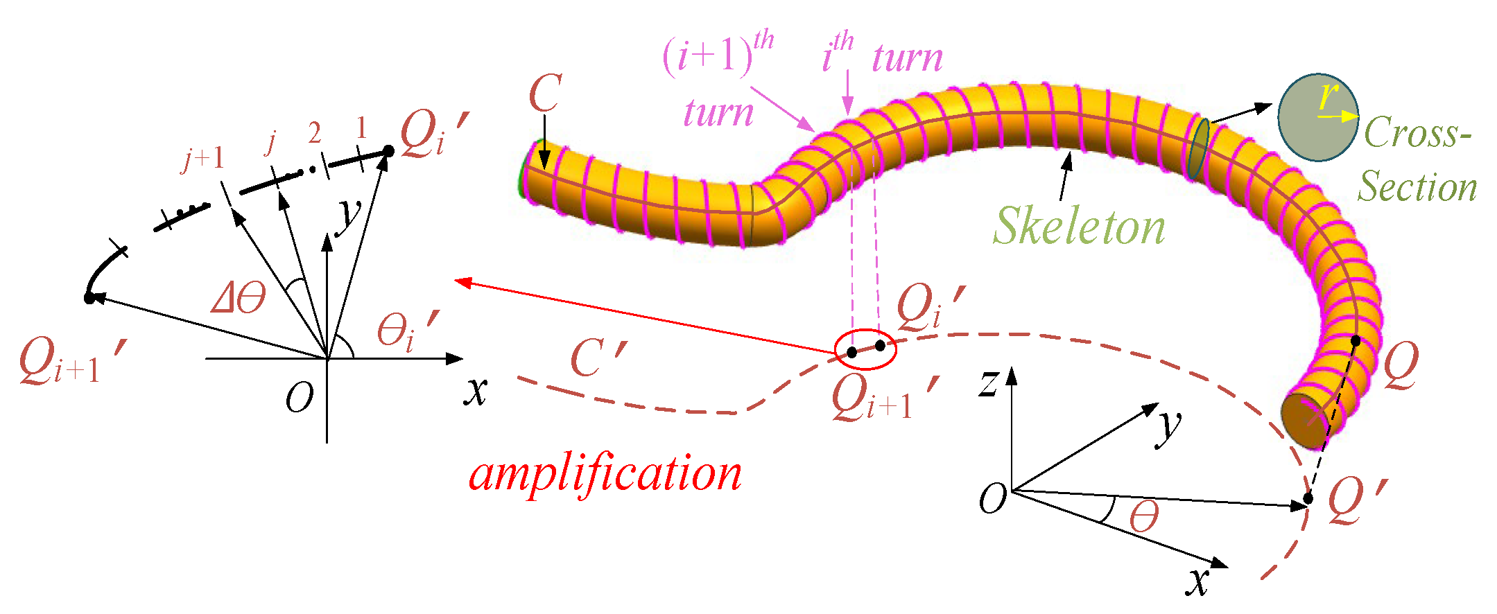
The winding coils are made by winding the winding wire along the skeleton, and the spatial position of each winding coil turn can be positioned according to the geometric centerline of the skeleton. Therefore, the geometric centerline equation is established. Additionally, a three-dimensional coordinate system is established, as shown in Figure 2. The space coordinate equation of skeleton centerline C is (α(θ), β(θ), and γ(θ)). Here, r is the radius of the circular section of the skeleton, Q is the point on line C, Q′ is the projection of point Q onto the xOy plane, and θ is the angle between line OQ′ and the x-axis. The geometric center of each turn is on line C. Q_i′ and Q_i+1′ are the projections of the geometric center of the ith turn and the (i+1)^th turn onto the xOy plane, respectively. Assume that N turns of the coil are evenly distributed along the skeleton and that the centerline is equally divided into N parts. The angle θ between the ith turn and the (i+1)^th turn is composed of infinitesimal isometric Δθ units, as shown in Figure 2, that is, θ_ij = θ_i + jΔθ. Keep increasing j until Equation (1) holds true; this value is known as J. The J value that makes the first expression of Equation (1) true is then substituted into θ_i + JΔθ, which is equal to the angle between the ith turn and the (i+1)^th turn. Here, δ is a number that goes to zero. The coordinates of the N equinoxes of line C can be quickly computed using Equations (1) and (2). Then, we can quickly calculate the coordinates of the geometric center of all the turns of the wound coil.

$$\left\{\begin{array}{c}\left|{\displaystyle \frac{L}{N-1}}-{\displaystyle \sum _{j=1,2,\dots J}}\sqrt{{\left({\alpha }^{\prime }\left({\theta }_{\mathit{ij}}\right)\right)}^2+({{\beta }^{\prime }\left({\theta }_{\mathit{ij}}\right))}^2+({{\gamma }^{\prime }\left({\theta }_{\mathit{ij}}\right))}^2}\Delta \theta \right|<\delta \\ {\theta }_{\mathit{ij}}={\theta }_i+j\Delta \theta \end{array}\right.$$

(1)

θ_i+1 = θ_i + JΔθ

(2)

where L is the length of line C. θ_i and θ_i+1 are the angles corresponding to the ith turn and the (i+1)^th turn, respectively. J in (2) is the value that makes (1) true.

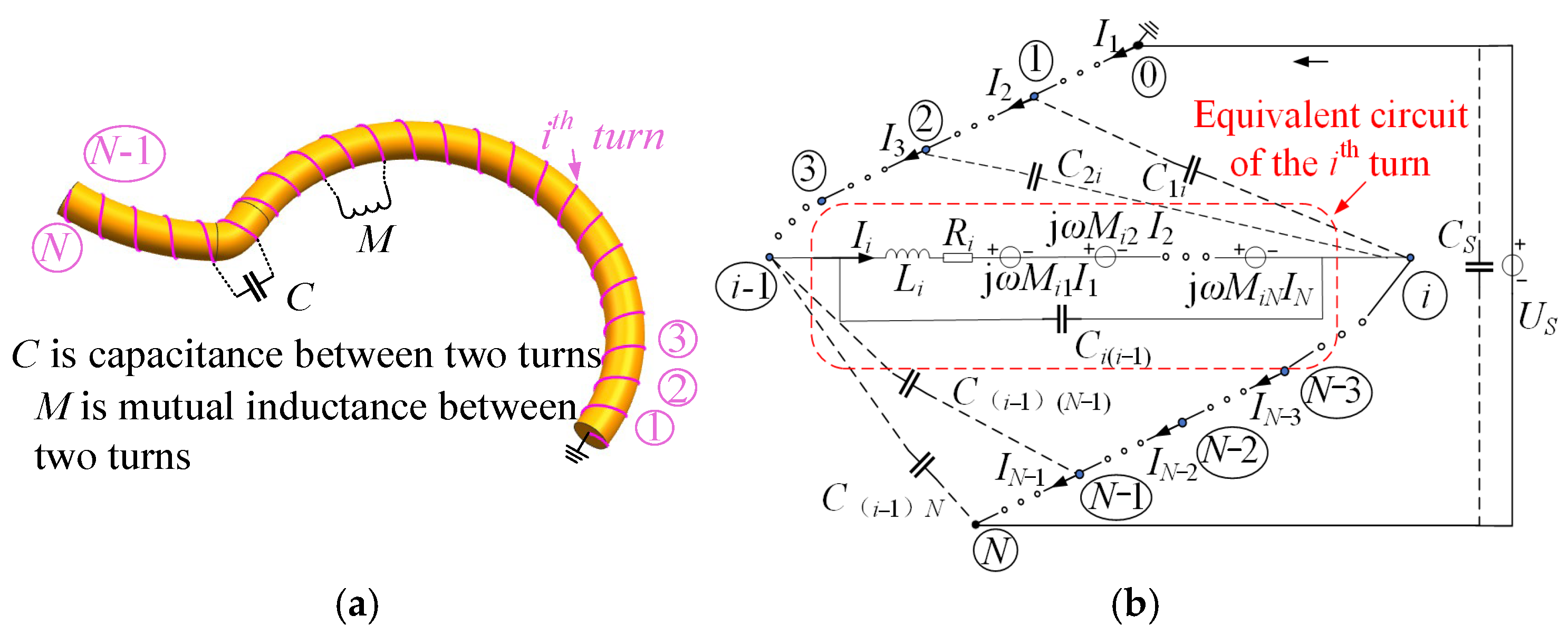
The coil is divided into many units to calculate the characteristics and electrical parameters of coils with arbitrary shapes at different frequencies, where each turn of the wound coil is a unit. Additionally, each turn is numbered in the direction in which the coil potential decreases/increases, as shown in Figure 3. The head end of the first turn is connected to the reference ground, and the tail end of the ith turn is connected to the head end of the (i+1)^th turn. ①, ②, ③ … are the serial number of the tail ends of the first turn, the second turn, the third turn,… and the ith turn, respectively. The equivalent circuits of the ith turn are highlighted by the red dotted line, and I_i is the current coming out of i − 1. C_ij and M_ij are the capacitance and mutual inductance between the ith turn and jth turn, respectively, while L_i and R_i are the self-inductance and resistance of the ith turn, respectively. C_S, I_S, and U_S are the parasitic capacitance of the impedance analyzer probe, input current, and input voltage of the impedance analyzer, respectively.

$$\mathit{Mij}={\left({\displaystyle \frac{2\mathit{\pi r}}{N_1}}\right)}^2{\displaystyle \frac{{\mu }_0}{4\pi }}{\displaystyle {\sum }_{h=1}^{h=N_1}}{\displaystyle {\sum }_{g=1}^{g=N_1}}{\displaystyle \frac{x^{\prime }(i,g)x^{\prime }(j,h)+y^{\prime }(i,g)y^{\prime }(j,h)+z^{\prime }(i,g)z^{\prime }(j,h)}{\sqrt{{\left(\mathit{Xij}\right)}^2+{\left(\mathit{Yij}\right)}^2+{\left(\mathit{Zij}\right)}^2}\sqrt{{\left(x^{\prime }(i,g)\right)}^2+{\left(y^{\prime }(i,g)\right)}^2+{\left(z^{\prime }(i,g)\right)}^2}\sqrt{{\left(x^{\prime }(j,h)\right)}^2+{\left(y^{\prime }(j,h)\right)}^2+{\left(z^{\prime }(j,h)\right)}^2}}}$$

(3)

$$\left\{\begin{array}{c}x\left(i,t\right)=\alpha \left({\theta }_i\right)+{\displaystyle \frac{r}{\sqrt{{\left({\beta }^{\prime }\left({\theta }_i\right)\right)}^2+{\left({\alpha }^{\prime }\left({\theta }_i\right)\right)}^2}}}\left[{\beta }^{\prime }\left({\theta }_i\right)\cos \left({\displaystyle \frac{2\pi }{N_1}}t\right)+{\displaystyle \frac{\sin \left(\frac{2\pi }{N_1}t\right){\alpha }^{\prime }\left({\theta }_i\right){\gamma }^{\prime }\left({\theta }_i\right)}{\sqrt{{\left({\beta }^{\prime }\left({\theta }_i\right)\right)}^2+{\left({\alpha }^{\prime }\left({\theta }_i\right)\right)}^2+{\left({\gamma }^{\prime }\left({\theta }_i\right)\right)}^2}}}\right]\\ y\left(i,t\right)=\beta \left({\theta }_i\right)-{\displaystyle \frac{r}{\sqrt{{\left({\beta }^{\prime }\left({\theta }_i\right)\right)}^2+{\left({\alpha }^{\prime }\left({\theta }_i\right)\right)}^2}}}[{\alpha }^{\prime }\left({\theta }_i\right)\cos \left({\displaystyle \frac{2\pi }{N_1}}t\right)-{\displaystyle \frac{\sin \left(\frac{2\pi }{N_1}t\right){\beta }^{\prime }\left({\theta }_i\right){\gamma }^{\prime }\left({\theta }_i\right)}{\sqrt{{\left({\beta }^{\prime }\left({\theta }_i\right)\right)}^2+{\left({\alpha }^{\prime }\left({\theta }_i\right)\right)}^2+{\left({\gamma }^{\prime }\left({\theta }_i\right)\right)}^2}}}]\\ z\left(i,t\right)=\gamma \left({\theta }_i\right)-r\left[{\displaystyle \frac{\sin \left(\frac{2\pi }{N_1}t\right)\left(\sqrt{{\left({\beta }^{\prime }\left({\theta }_i\right)\right)}^2+{\left({\alpha }^{\prime }\left({\theta }_i\right)\right)}^2}\right)}{\sqrt{{\left({\beta }^{\prime }\left({\theta }_i\right)\right)}^2+{\left({\alpha }^{\prime }\left({\theta }_i\right)\right)}^2+{\left({\gamma }^{\prime }\left({\theta }_i\right)\right)}^2}}}\right]\left(1\le t\le N_1\right)({\left({\beta }^{\prime }\left({\theta }_i\right)\right)}^2+{\left({\alpha }^{\prime }\left({\theta }_i\right)\right)}^2\ne 0)\end{array}\right.$$

(4)

$$\left\{\begin{array}{c}\mathit{Xij}=x(i,g)-x(j,h)\\ \mathit{Yij}=y(i,g)-y(j,h)\\ \mathit{Zij}=z(i,g)-z(j,h)\end{array}\right.$$

(5)

If ${\left({\beta }^{\prime }\left({\theta }_i\right)\right)}^2+{\left({\alpha }^{\prime }\left({\theta }_i\right)\right)}^2=0$, x(i,t) = r  $\sin \left({\displaystyle \frac{2\pi }{N_1}}t\right), y\left(i,t\right)=$ r $\cos \left({\displaystyle \frac{2\pi }{N_1}}t\right),$z = γ(θ_i) (1 ≤ t ≤ N₁). where μ₀ represents the vacuum permeability, while (x′(i,t), y′(i,t), and z′(i,t)) are the derivatives of (x(i,t), y(i,t), and z(i,t)) with respect to t.

The self-inductance L_i can be calculated according to the following equation [37]

$$L_i={\mu }_{0}r[\left(1-{\displaystyle \frac{{r_l}^2}{4r^2}}\mathit{ln}{\displaystyle \frac{8r}{r_l}}+{\displaystyle \frac{{r_l}^2}{2r^2}}\right)\mathit{ln}{\displaystyle \frac{8r}{r_l}}-2-{\displaystyle \frac{{r_l}^2}{16r^2}}]$$

(6)

where r_l is the radius of the wound wire.

The resistance R_i and the capacitance C_ij between the ith turn and the jth turn are calculated according to reference [38]. The relationship between the current and voltage of the ith turn and that of the (i−1)^th turn is

$$\left\{\begin{array}{c}{U}_{i-1}-U_i=\left(\mathrm{j}\omega L_i+R_i\right)I_i+{\sum }_{j=1,j\ne i}^{j=N}\mathrm{j}\omega M_{i,j}{I}_j\\ \begin{array}{c}{I}_1=I_S+\mathrm{j}\omega C_S{U}_N\\ I_{i-1}-I_i={\sum }_{j=1,j\ne i-1}^{j=N}\mathrm{j}\omega C_{i-1,j}\left(U_{i-1}-U_j\right), i>1\end{array}\end{array}\right.$$

(7)

where U_i is the voltage at the end of the ith turn. Z_i = jωL_i + R_i, and ω = 2πf. f is the frequency.

Equation (7) is converted to the matrix form

$$\mathit{A}\left[\begin{array}{c}{U}_1\\ U_2\\ \begin{array}{c}⋮\\ U_{N-1}\\ U_N\end{array}\end{array}\right]=\mathit{Z}\left[\begin{array}{c}{I}_1\\ I_2\\ \begin{array}{c}⋮\\ I_{N-1}\\ I_N\end{array}\end{array}\right]$$

(8)

$$\mathit{B}\left[\begin{array}{c}{I}_1\\ I_2\\ \begin{array}{c}⋮\\ I_{N-1}\\ I_N\end{array}\end{array}\right]=\left[\begin{array}{c}{I}_S\\ 0\\ \begin{array}{c}⋮\\ 0\\ 0\end{array}\end{array}\right]+\mathit{C}\left[\begin{array}{c}{U}_1\\ U_2\\ \begin{array}{c}⋮\\ U_{N-1}\\ U_N\end{array}\end{array}\right]$$

(9)

$$\mathit{A} = \left[\begin{array}{ccc}-1& 0& \begin{array}{ccc}\dots & 0& 0\end{array}\\ 1& -1& \begin{array}{ccc}\dots & 0& 0\end{array}\\ \begin{array}{c}0\\ ⋮\\ 0\end{array}& \begin{array}{c}1\\ \dots \\ 0\end{array}& \begin{array}{ccc}\begin{array}{c}\ddots \\ \cdots \\ \dots \end{array}& \begin{array}{c}0\\ -1\\ 1\end{array}& \begin{array}{c}0\\ 0\\ -1\end{array}\end{array}\end{array}\right]$$

(10)

$$\mathit{Z}=\left[\begin{array}{ccc}{Z}_1& \mathrm{j}\omega M_{1,2}& \begin{array}{ccc}\dots & \mathrm{j}\omega M_{1,N-1}& \mathrm{j}\omega M_{1,N}\end{array}\\ \mathrm{j}\omega M_{1,2}& Z_2& \begin{array}{ccc}\dots & \mathrm{j}\omega M_{2,N-1}& \mathrm{j}\omega M_{2,N}\end{array}\\ \begin{array}{c}\dots \\ ⋮\\ \mathrm{j}\omega M_{N,1}\end{array}& \begin{array}{c}\dots \\ \dots \\ \mathrm{j}\omega M_{N,2}\end{array}& \begin{array}{ccc}\begin{array}{c}\ddots \\ \dots \\ \dots \end{array}& \begin{array}{c}\dots \\ Z_{N-1}\\ \mathrm{j}\omega M_{N,N-1}\end{array}& \begin{array}{c}\mathrm{j}\omega M_{1,2}\\ \mathrm{j}\omega M_{1,2}\\ Z_N\end{array}\end{array}\end{array}\right]$$

(11)

$$\mathit{B}=\left[\begin{array}{ccc}1& 0& \begin{array}{ccc}\dots & 0& 0\end{array}\\ 1& -1& \begin{array}{ccc}\dots & 0& 0\end{array}\\ \begin{array}{c}0\\ ⋮\\ 0\end{array}& \begin{array}{c}1\\ \dots \\ 0\end{array}& \begin{array}{ccc}\begin{array}{c}\ddots \\ \dots \\ \dots \end{array}& \begin{array}{c}0\\ -1\\ 1\end{array}& \begin{array}{c}0\\ 0\\ -1\end{array}\end{array}\end{array}\right]$$

(12)

$$\mathit{C}=\left[\begin{array}{ccc}0& 0& \begin{array}{ccc}\dots & 0& \mathrm{j}\omega C_{1,N} \end{array}\\ \mathrm{j}\omega C_{2,1}& -\mathrm{j}\omega {\sum }_{j=1}^{j=N}{C}_{2,j}& \begin{array}{ccc}\dots & \cdots & \mathrm{j}\omega C_{2,N}\end{array}\\ \begin{array}{c}\mathrm{j}\omega C_{3,1}\\ ⋮\\ \mathrm{j}\omega C_{N,1}\end{array}& \begin{array}{c}\mathrm{j}\omega C_{3,2}\\ \dots \\ \mathrm{j}\omega C_{N,2}\end{array}& \begin{array}{ccc}\begin{array}{c}\ddots \\ \dots \\ \dots \end{array}& \begin{array}{c}\dots \\ \dots \\ \dots \end{array}& \begin{array}{c}\mathrm{j}\omega C_{3,N}\\ ⋮\\ -\mathrm{j}\omega {\sum }_{j=1}^{j=N}{C}_{N,j}\end{array}\end{array}\end{array}\right]$$

(13)

Equation (9) can be transformed to the following form:

$$\left[\begin{array}{c}{I}_1\\ I_2\\ \begin{array}{c}⋮\\ I_{N-1}\\ I_N\end{array}\end{array}\right]={\mathit{B}}^{-\mathbf{1}}\mathit{C}\left[\begin{array}{c}{U}_1\\ U_2\\ \begin{array}{c}⋮\\ U_{N-1}\\ U_N\end{array}\end{array}\right]+{\mathit{B}}^{-\mathbf{1}}\left[\begin{array}{c}{I}_S\\ 0\\ \begin{array}{c}⋮\\ 0\\ 0\end{array}\end{array}\right]$$

(14)

Place (14) into (8)

$$(\mathit{A}-\mathit{Z}{\mathit{B}}^{-\mathbf{1}}\mathit{C})\left[\begin{array}{c}{U}_1\\ U_2\\ \begin{array}{c}⋮\\ U_{N-1}\\ U_N\end{array}\end{array}\right]={\mathit{ZB}}^{-\mathbf{1}}\left[\begin{array}{c}{I}_S\\ 0\\ \begin{array}{c}⋮\\ 0\\ 0\end{array}\end{array}\right]$$

(15)

Convert the coefficient of ${\left[U_1,U_2,U_3\dots U_N\right]}^T$ to the upper triangular matrix

$$\mathit{E}\left[\begin{array}{c}{U}_1\\ U_2\\ \begin{array}{c}⋮\\ U_{N-1}\\ U_N\end{array}\end{array}\right]={\mathit{D}}^{-\mathbf{1}}{\mathit{ZB}}^{-\mathbf{1}}\left[\begin{array}{c}{I}_S\\ 0\\ \begin{array}{c}⋮\\ 0\\ 0\end{array}\end{array}\right]=\mathit{F}{\mathit{I}}_{\mathit{S}}$$

(16)

where E is the upper triangular matrix, with (A − ZB⁻¹C) = DE. The input impedance Z_I affected by the frequency can be calculated according to the following equation

$$Z_I(\omega )={\displaystyle \frac{U_N}{I_S}}={\displaystyle \frac{F_N}{E_{N,N}}}=R_e(f)+\mathrm{j}\mathsf{\omega }{L}_e(f)$$

(17)

where R_e(f) and L_e(f) are the equivalent resistor and equivalent inductance, respectively.

2.2. PCB Coils with a Complex Structure

The PCB coils are mostly composed of multiple straight lines and curved lines. The ends of the lines should be numbered quickly to calculate the electrical parameters of the PCB coil quickly. To better illustrate the calculation method, a PCB coil with a complex structure obtained from [4] is taken as an example, as shown in Figure 1c.

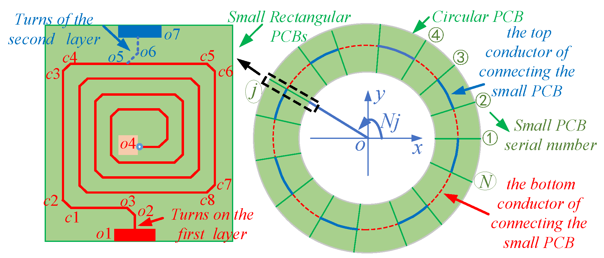
Figure 4 shows a schematic diagram of Figure 1c. The PCB coil is composed of two large circular ring PCBs and several small rectangular PCBs, as shown in Figure 4. These rectangular PCBs are sandwiched vertically between the two circular ring PCBs, and the wiring printed on the circular ring PCBs is used to connect these rectangular PCBs. Therefore, all the rectangular PCBs are connected to form a path. Additionally, every rectangular PCB has two layer turns. The spatial position of each line segment that makes up the PCB coil should be located quickly to quickly calculate the input impedance of the PCB coils.

First, the number of rectangular PCBs in a certain direction is considered. The origin of the reference coordinate system is located at the center of the coil, and the z-axis coincides with the center line. The x-axis coincides with the centerline of the projection of the first rectangular PCB on the circular ring PCB. Then, the coordinates of the ends of the outermost wiring on the upper-layer PCB of the first rectangular PCB are written out, where the wiring distance on the rectangular PCB is assumed to be b and the number of turns per layer and the number of layers in the rectangular PCB are assumed to be n and m, respectively. Since each turn has four corners and the PCB production angle is mostly obtuse, there are two points in each corner. As Figure 4 shows, c1, c2, c3, c4, c5, …, o1, o2,… are the serial numbers of the two ends of the wiring segments that form the coil. First, note the coordinates of the two ends of the outermost line on the first rectangular PCB according to its size. The serial number of the ends of the wiring segment in the small PCB is m*(8*n + 6), so the coordinates of all the ends can be calculated according to the coordinates of the ends of the outermost wiring. Additionally, the coordinates of two ends of the wiring segments on the jth PCB can be obtained by rotating the end coordinates on the first PCB around the z-axis. Equation (18) is taken as an example to illustrate the calculation method. The spatial coordinates of the ith (i ∉ {o₁, o₂, o₃,o₅, o₆, o₇}) end on the first layer of the jth small PCB can be quickly calculated according to the equation

$$\left\{\begin{array}{c}\mathit{if} i<\left(8\ast \mathrm{n}+3\right) \mathit{and} \left(i-3\right) \mathit{mod} 8=k\\ \mathit{Nj}={\displaystyle \frac{2\pi }{N_P}}\left(j-1\right) \\ \begin{array}{c}{x}_{\mathit{ji}}=\left(x_k\pm \left[{\displaystyle \frac{\left(i-3\right)}{8}}\right]\ast b\right)\ast \cos \left(\mathit{Nj}\right)-y_k\sin \left(\mathit{Nj}\right)\\ y_{\mathit{ji}}=\left(x_k\pm \left[{\displaystyle \frac{\left(i-3\right)}{8}}\right]\ast b\right)\ast \sin \left(\mathit{Nj}\right)+y_k\ast \cos \left(\mathit{Nj}\right)\\ z_{\mathit{ji}}=z_k\pm \left[\left(i-3\right)/8\right]\ast b\end{array}\end{array}\right.$$

(18)

where x_k, y_k, and z_k are the coordinate of the ends of the outermost line on the upper layer of the first rectangular PCB; N_P is the total number of rectangular PCBs; and Nj represents the angle of the jth small PCB in the Cartesian coordinate system. The spatial coordinates of the ith (i ∈ {o₁, o₂, o₃,o₅, o₆, o₇}) end on the first layer of the jth small PCB can be quickly calculated according to the equation

$$\left\{\begin{array}{c}\mathit{if} i>\left(8\ast \mathrm{n}+3\right) \mathit{or} i<4 \\ \mathit{Nj}={\displaystyle \frac{2\pi }{N_P}}\left(j-1\right) \\ \begin{array}{c}{x}_{\mathit{ji}}=x_i\ast \cos \left(\mathit{Nj}\right)-y_i\sin \left(\mathit{Nj}\right)\\ y_{\mathit{ji}}=x_i\ast \sin \left(\mathit{Nj}\right)+y_i\ast \cos \left(\mathit{Nj}\right)\\ z_{\mathit{ji}}=z_i\end{array}\end{array}\right.$$

(19)

$$M={\displaystyle \frac{{\mu }_0}{4\pi }}{\sum }_{j=1}^{j=N_2}{\sum }_{i=1}^{i=N_1}{\displaystyle \frac{\left({x_B-x}_A\right)\left({x_D-x}_C\right)+\left({y_B-y}_A\right)\left({y_D-y}_C\right)+\left({z_B-z}_A\right)\left({z_D-z}_C\right)}{N_1{N}_2\sqrt{{\left({x_i-x}_j\right)}^2+{\left({y_i-y}_j\right)}^2+{\left({z_i-z}_j\right)}^2}}}$$

(20)

$$\left\{\begin{array}{c}{x}_i=x_A+{\displaystyle \frac{x_B-x_A}{N_1}}(i-0.5)\\ y_i=y_A+{\displaystyle \frac{y_B-y_A}{N_1}}(i-0.5)\\ z_i=z_A+{\displaystyle \frac{z_B-z_A}{N_1}}(i-0.5)\end{array}\right.,\left\{\begin{array}{c}{x}_j=x_C+{\displaystyle \frac{x_D-x_C}{N_2}}(j-0.5)\\ y_j=y_C+{\displaystyle \frac{y_D-y_C}{N_2}}(j-0.5)\\ z_j=z_C+{\displaystyle \frac{z_D-z_C}{N_2}}(j-0.5)\end{array}\right.$$

(21)

where A(x_A, y_A, z_A), B(x_B, y_B, z_B), C(x_C, y_C, z_C), and D(x_D, y_D, z_D) are the coordinates of the ends of the two wiring segments, while x_i, y_i, z_i and x_j, y_j, z_j are the coordinates of the ith and jth elementary parts, respectively.

The coordinates of the ends of the wiring segments on the entire coil can be quickly calculated. Since the calculation method is based on the lumped parameter method and considers electromagnetic wavelength, the unit consists of a straight segment and the adjacent segment forming an obtuse angle, such as line segments o1o2o3 and o3c1c2. The last unit of each rectangular PCB contains only one line segment, namely line segment o6o7. Discrete two straight conductors at arbitrary positions in space into equal elementary parts (N₁ and N₂, respectively). According to Newman’s law, the mutual inductance between two wires can be calculated using Equations (20) and (21). The self-inductance of the ith PCB wiring can be calculated using the following equation [34]:

$$L_i={\displaystyle \frac{{\mu }_0{l}_i}{2\pi }}(\mathit{ln}{\displaystyle \frac{4l_i}{k_1}}-1)$$

(22)

where l_i is the length of the ith PCB wiring segment and can be calculated using the coordinates of the two ends of the ith line segment, while k₁ represents the width of the PCB traces.

The capacitance C_ij between the ith and jth PCB wiring segments can be calculated using the equation

$$C_{\mathit{ij}}=(\epsilon w^2)/{(\mathit{sin}{\theta }_{\mathit{ij}}d}_{\mathit{ij}})({\theta }_{\mathit{ij}}\ne 0) \mathrm{and} (C_{\mathit{ij}}=(\epsilon w{l}_{\mathit{min}})/(d_{\mathit{ij}})({\theta }_{\mathit{ij}}=0)$$

(23)

where θ_ij is the angle between the ith and jth segments. d_ij is the shortest distance between the ith segment and the jth segments, and w is the width of the PCB trace winding. l_min is the length of the projection area between two parallel line segments. The dielectric constant ε can be obtained from tables based on the PCB substrate material.

The unit resistance R_o can be quickly calculated based on a two-dimensional model using the frequency and size parameter scanning function of the ANSYS simulation software 2022R1. Although it is difficult to calculate the electrical parameters throughout a coil with dense winding and an irregular frame shape using electromagnetic simulation software, the model can obtain thousands of resistance data tables for different sizes and frequencies within a few minutes. The resistance R_i can be calculated using the following equation:

$$R_i={R_{o}l}_i$$

(24)

Then, the mutual inductance, resistance, inductance, and capacitance matrix can be calculated according to the above derivation of the parameter calculation equation. Moreover, the input impedance of the PCB coil with a complex structure can be calculated using (17).

2.3. Two Coupled Coils with a Complex Structure

Electrical equipment often has different types of coupled coils, as shown in Figure 1. The coils are coupled by the mutual inductance and stray capacitance between their turns. Additionally, the port characteristics of the coil are affected by its coupled coil. The method to quickly and accurately calculate the interaction between coupled coils is given in this section.

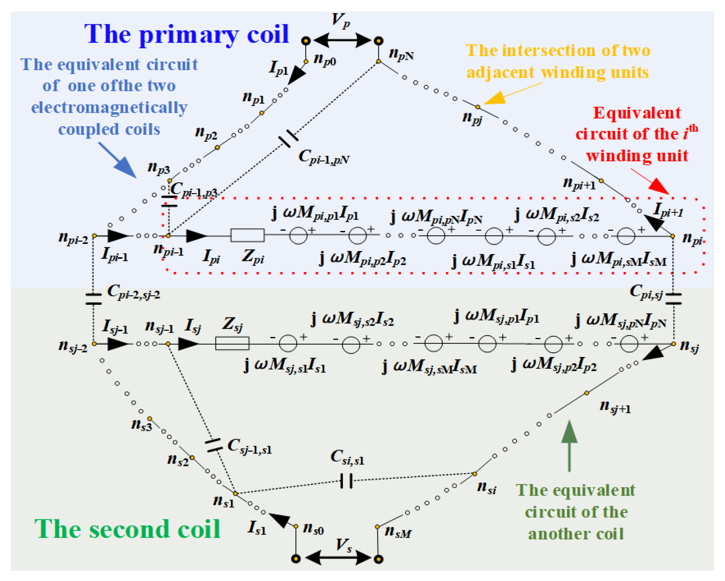
Figure 5 shows the equivalent circuit of two coupled coils. The parasitic parameters between two turns of the two coupled coils are considered to obtain more accurate calculation results. The coils are divided into many winding units, and the coupling between each winding unit is depicted in Figure 5, where the parameters with the subscripts p and s represent those of the primary and secondary coils, respectively. As shown in Figure 5, the circuits with blue and green backgrounds represent the equivalent circuits of the first and second coils, respectively. The first coil is divided into N winding units, while the second coil is divided into M winding units. n_p0 and n_s0 represent the reference of the first and second coils, respectively. n_pi (i ≠ 0 and N) and n_sj (j ≠ 0 and M) represent the intersection between two adjacent winding units of the first and second coils, respectively. n_pN and n_sM are the tail ends of the Nth and Mth winding units of the first and second coils, respectively. C_pi,pj and M_pi,pj are the parasitic capacitance and mutual inductance between the ith and jth winding units of the first coil, respectively, while C_pi,sj and M_pi,sj are the parasitic capacitance and mutual inductance between the ith winding unit of the first coil and the jth winding unit of the second coil, respectively. I_pi and I_sj represent the branch current of the ith winding unit of the first coil and the jth winding unit of the second coil, respectively, while Z_pi and Z_sj represent the branch impedance of the ith winding unit of the first coil and the jth winding unit of the second coil, respectively. Z_i = r_i + jωL_i, where r_i and L_i are the resistor and the inductance of the ith winding unit, respectively. V_P and V_S are the port voltages of the first and second coils, respectively. I_P and I_S are the port current of the first coil and the second coil, respectively.

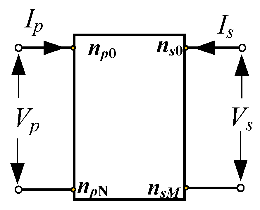
The two coupled coils can be viewed as a two-port network to quickly calculate their port frequency characteristics of the two coupled coils, as shown in Figure 6. According to Figure 5 and Figure 6, the electrical relationships of the first turn segment of the primary coil (p1) can be written as

$$p1: \left\{\begin{array}{c}-V_{p1}=Z_{p1}{I}_{p1}-\mathrm{j}\omega {\sum }_{i=2}^{i=N}{M}_{p1,\mathit{pi}}{I}_{\mathit{pi}}-\mathrm{j}\omega {\sum }_{j=1}^{j=M}{ M}_{p1,\mathit{sj}}{I}_{\mathit{sj}}\\ I_{p1}=I_p\end{array}\right.$$

(25)

The electrical relationships of the ith (i ≥ 2) turn segment of the primary coil (pi) can be written as

$$\mathit{pi}(i \ge 2): \left\{\begin{array}{c}{V}_{p\left(i-1\right)}-V_{\mathit{pi}}=Z_{\mathit{pi}}{I}_{\mathit{pi}}-\mathrm{j}\omega {\sum }_{j=2,j\ne i}^{j=N}{ M}_{\mathit{pi},\mathit{pj}}{·I}_{\mathit{pj}}-\mathrm{j}\omega {\sum }_{j=1}^{j=M}{M}_{\mathit{pi},\mathit{sj}}{·I}_{\mathit{sj}}\\ I_{p\left(i-1\right)}-I_{\mathit{pi}}=\mathrm{j}\omega {\sum }_{j=1,j\ne i-1}^{j=N}{C}_{p\left(i-1\right),\mathit{pj}}\left(V_{p\left(i-1\right)}-V_{\mathit{pj}}\right)+\mathrm{j}\omega {\sum }_{j=1}^{j=M}{C}_{p\left(i-1\right),\mathit{sj}}\left(V_{p\left(i-1\right)}-V_{\mathit{sj}}\right)\end{array}\right.$$

(26)

The electrical relationships of the first turn segment of the second coil (s1) can be written as

$$s1: \left\{\begin{array}{c}-V_{s1}=Z_{s1}{I}_{s1}-\mathrm{j}\omega {\sum }_{i=2}^{i=M}{M}_{s1,\mathit{si}}{·I}_{\mathit{si}}-\mathrm{j}\omega {\sum }_{j=1}^{j=N}{M}_{s1,\mathit{pj}}{·I}_{\mathit{pj}}\\ I_{s1}=I_s\end{array}\right.$$

(27)

The electrical relationships of the ith (i ≥ 2) turn segment of the second coil v(si) can be written as

$$\mathit{si}\left(i\ge 2\right): \left\{\begin{array}{c}{V}_{s(i-1)}-V_{\mathit{si}}=Z_{\mathit{si}}{I}_{\mathit{si}}-\mathrm{j}\omega {\sum }_{j=2,j\ne i}^{j=M}{ M}_{\mathit{si},\mathit{sj}}{·I}_{\mathit{sj}}-\mathrm{j}\omega {\sum }_{j=1}^{j=N}{M}_{\mathit{si},\mathit{pj}}{·I}_{\mathit{pj}}\\ I_{s(i-1)}-I_{\mathit{si}}=\mathrm{j}\omega {\sum }_{j=1,j\ne i-1}^{j=M}{C}_{s\left(i-1\right),\mathit{sj}}\left(V_{s\left(i-1\right)}-V_{\mathit{sj}}\right)+\mathrm{j}\omega {\sum }_{j=1}^{j=N}{C}_{s\left(i-1\right),\mathit{pj}}\left(V_{s\left(i-1\right)}-V_{\mathit{pj}}\right)\end{array}\right.$$

(28)

Convert the first equation of Equations (25)–(28) into the matrix form

$$\mathit{Z}\left[\begin{array}{c}{I}_{p1}\\ I_{p2}\\ \begin{array}{c}⋮\\ I_{\mathit{pN}}\\ \begin{array}{c}{I}_{s1}\\ I_{s2}\\ \begin{array}{c}⋮\\ I_{\mathit{sM}}\end{array}\end{array}\end{array}\end{array}\right]=\mathit{E}\mathbf{1}\left[\begin{array}{c}{V}_{p1}\\ V_{p2}\\ \begin{array}{c}⋮\\ V_{\mathit{pN}}\\ \begin{array}{c}{V}_{s1}\\ V_{s2}\\ \begin{array}{c}⋮\\ V_{\mathit{sM}}\end{array}\end{array}\end{array}\end{array}\right]$$

(29)

Convert the second equation of Equations (25)–(28) into the matrix form

$$\mathit{E}\mathbf{2}\left[\begin{array}{c}{I}_{p1}\\ I_{p2}\\ \begin{array}{c}⋮\\ I_{\mathit{pN}}\\ \begin{array}{c}{I}_{s1}\\ I_{s2}\\ \begin{array}{c}⋮\\ I_{\mathit{sM}}\end{array}\end{array}\end{array}\end{array}\right]=\left[\begin{array}{c}{I}_p\\ 0\\ \begin{array}{c}⋮\\ 0\\ \begin{array}{c}{I}_s\\ 0\\ \begin{array}{c}⋮\\ 0\end{array}\end{array}\end{array}\end{array}\right]-\mathrm{j}\omega \mathit{C}\left[\begin{array}{c}{V}_{p1}\\ V_{p2}\\ \begin{array}{c}⋮\\ V_{\mathit{pN}}\\ \begin{array}{c}{V}_{s1}\\ V_{s2}\\ \begin{array}{c}⋮\\ V_{\mathit{sM}}\end{array}\end{array}\end{array}\end{array}\right]$$

(30)

$$\mathit{Z}=\left[\begin{array}{cc}\begin{array}{ccc}{Z}_{p1}& -\mathrm{j}\omega M_{p1,p2}& \begin{array}{cc}\dots & -\mathrm{j}\omega M_{p1,\mathit{pN}}\end{array}\\ -\mathrm{j}\omega M_{p2,p1}& Z_{p2}& \begin{array}{cc}\dots & -\mathrm{j}\omega M_{p2,\mathit{pN}}\end{array}\\ \begin{array}{c}⋮\\ -\mathrm{j}\omega M_{\mathit{pN},p1}\end{array}& \begin{array}{c}⋮\\ -\mathrm{j}\omega M_{\mathit{pN},p2}\end{array}& \begin{array}{cc}\begin{array}{c}\dots \\ \dots \end{array}& \begin{array}{c}⋮\\ Z_{\mathit{pN}}\end{array}\end{array}\end{array}& \begin{array}{ccc}-\mathrm{j}\omega M_{p1,s1}& -\mathrm{j}\omega M_{p1,s2}& \begin{array}{cc}\dots & -\mathrm{j}\omega M_{p1,\mathit{sM}}\end{array}\\ -\mathrm{j}\omega M_{p2,s1}& -\mathrm{j}\omega M_{p2,s2}& \begin{array}{cc}\dots & -\mathrm{j}\omega M_{p2,\mathit{sM}}\end{array}\\ \begin{array}{c}⋮\\ -\mathrm{j}\omega M_{\mathit{pN},s1}\end{array}& \begin{array}{c}⋮\\ -\mathrm{j}\omega M_{\mathit{pN},s2}\end{array}& \begin{array}{cc}\begin{array}{c}\dots \\ \dots \end{array}& \begin{array}{c}⋮\\ -\mathrm{j}\omega M_{\mathit{pN},\mathit{sM}}\end{array}\end{array}\end{array}\\ \begin{array}{ccc}-\mathrm{j}\omega M_{s1,p1}& -\mathrm{j}\omega M_{s1,p2}& \begin{array}{cc}\dots & -\mathrm{j}\omega M_{s1,\mathit{pN}}\end{array}\\ -\mathrm{j}\omega M_{s2,p1}& -\mathrm{j}\omega M_{s2,p2}& \begin{array}{cc}\dots & -\mathrm{j}\omega M_{s2,\mathit{pN}}\end{array}\\ \begin{array}{c}⋮\\ -\mathrm{j}\omega M_{\mathit{sM},p1}\end{array}& \begin{array}{c}⋮\\ -\mathrm{j}\omega M_{\mathit{sM},p2}\end{array}& \begin{array}{cc}\begin{array}{c}\dots \\ \dots \end{array}& \begin{array}{c}⋮\\ -\mathrm{j}\omega M_{\mathit{sM},\mathit{pN}}\end{array}\end{array}\end{array}& \begin{array}{ccc}{Z}_{s1}& -\mathrm{j}\omega M_{s1,s2}& \begin{array}{cc}\dots & -\mathrm{j}\omega M_{s1,\mathit{sM}}\end{array}\\ -\mathrm{j}\omega M_{s2,s1}& Z_{s2}& \begin{array}{cc}\dots & -\mathrm{j}\omega M_{s2,\mathit{sM}}\end{array}\\ \begin{array}{c}⋮\\ -\mathrm{j}\omega M_{\mathit{sM},s1}\end{array}& \begin{array}{c}⋮\\ -\mathrm{j}\omega M_{\mathit{sM},s2}\end{array}& \begin{array}{cc}\begin{array}{c}\dots \\ \dots \end{array}& \begin{array}{c}⋮\\ Z_{\mathit{sM}}\end{array}\end{array}\end{array}\end{array}\right]$$

(31)

$$\mathit{E}\mathbf{1}=\left[\begin{array}{cc}\begin{array}{ccc}\begin{array}{c}-1\\ 1\end{array}& \begin{array}{c}0\\ -1\end{array}& \begin{array}{c}\begin{array}{ccc}0& \dots & 0\end{array}\\ \begin{array}{ccc}0& \dots & 0\end{array}\end{array}\\ \begin{array}{c}0\\ ⋮\end{array}& \begin{array}{c}1\\ \dots \end{array}& \begin{array}{c}\begin{array}{ccc}-1& \dots & 0\end{array}\\ \begin{array}{ccc}\dots & \dots & ⋮\end{array}\end{array}\\ 0& \dots & \begin{array}{ccc}0& 1& -1\end{array}\end{array}& \mathbf{0}\\ \mathbf{0}& \begin{array}{ccc}\begin{array}{c}-1\\ 1\end{array}& \begin{array}{c}0\\ -1\end{array}& \begin{array}{c}\begin{array}{ccc}0& \dots & 0\end{array}\\ \begin{array}{ccc}0& \dots & 0\end{array}\end{array}\\ \begin{array}{c}0\\ ⋮\end{array}& \begin{array}{c}1\\ \dots \end{array}& \begin{array}{c}\begin{array}{ccc}-1& \dots & 0\end{array}\\ \begin{array}{ccc}\dots & \dots & ⋮\end{array}\end{array}\\ 0& \dots & \begin{array}{ccc}0& 1& -1\end{array}\end{array}\end{array}\right]$$

(32)

$$\mathit{C}=\left[\begin{array}{cc}\begin{array}{cc}\begin{array}{c}\begin{array}{c}\begin{array}{ccc}0& 0& \dots \\ C_{p1,p2}& {\mathit{C}}_{p2}& \dots \\ ⋮& ⋮& \dots \end{array}\\ \begin{array}{ccc}{C}_{\mathit{pi},p1}& C_{\mathit{pi},p2}& \dots \\ ⋮& ⋮& \dots \\ C_{\mathit{pN}-1,p2}& C_{\mathit{pN}-1,p2}& \dots \end{array}\end{array}\\ \begin{array}{c}\begin{array}{ccc}0& 0& \dots \\ C_{p1,s1}& C_{p2,s1}& \dots \\ ⋮& ⋮& \dots \end{array}\\ \begin{array}{ccc}{C}_{p1,\mathit{si}}& C_{p2,\mathit{si}}& \dots \\ ⋮& ⋮& \dots \\ C_{\mathit{sM}-1,p1}& C_{\mathit{sM}-1,p2}& \dots \end{array}\end{array}\end{array}& \begin{array}{c}\begin{array}{c}\begin{array}{ccc}\dots & \dots & \dots \\ C_{p1,\mathit{pj}}& \dots & C_{p1,\mathit{pN}}\\ ⋮& \dots & ⋮\end{array}\\ \begin{array}{ccc}{\mathit{C}}_{\mathit{pi}}& \dots & C_{\mathit{pi},\mathit{pN}}\\ ⋮& \dots & ⋮\\ C_{\mathit{pN}-1,\mathit{pj}}& \dots & {\mathit{C}}_{\mathit{pN}-1}\end{array}\end{array}\\ \begin{array}{c}\begin{array}{ccc}\dots & \dots & \dots \\ C_{\mathit{pj},s1}& \dots & C_{s1,\mathit{pN}}\\ ⋮& \dots & ⋮\end{array}\\ \begin{array}{ccc}{C}_{\mathit{pj},\mathit{si}}& \dots & C_{\mathit{pN},\mathit{si}}\\ ⋮& \dots & ⋮\\ C_{\mathit{sM}-1,\mathit{pj}}& \dots & C_{\mathit{sM}-1,\mathit{pN}}\end{array}\end{array}\end{array}\end{array}& \begin{array}{cc}\begin{array}{c}\begin{array}{c}\begin{array}{ccc}0& \dots & \dots \\ C_{p1,s1}& C_{p1,s2}& \dots \\ ⋮& ⋮& \dots \end{array}\\ \begin{array}{ccc}{C}_{\mathit{pi},s1}& C_{\mathit{pi},s2}& \dots \\ ⋮& ⋮& \dots \\ C_{\mathit{pN}-1,s1}& C_{\mathit{pN}-1,s2}& \dots \end{array}\end{array}\\ \begin{array}{c}\begin{array}{ccc}0& \dots & \dots \\ C_{s2,s1}& {\mathit{C}}_{s1}& \dots \\ ⋮& ⋮& \dots \end{array}\\ \begin{array}{ccc}{C}_{s1,\mathit{si}}& C_{s2,\mathit{si}}& \dots \\ ⋮& ⋮& \dots \\ C_{\mathit{sM}-1,s1}& C_{\mathit{sM}-1,s2}& \dots \end{array}\end{array}\end{array}& \begin{array}{c}\begin{array}{c}\begin{array}{ccc}\dots & \dots & 0\\ C_{p1,\mathit{sj}}& \dots & C_{p1,\mathit{sM}}\\ ⋮& \dots & ⋮\end{array}\\ \begin{array}{ccc}{C}_{\mathit{pi},\mathit{sj}}& \dots & C_{\mathit{pi},\mathit{sM}}\\ ⋮& \dots & ⋮\\ C_{\mathit{pN}-1,\mathit{sj}}& \dots & C_{\mathit{pN}-1,\mathit{sM}}\end{array}\end{array}\\ \begin{array}{c}\begin{array}{ccc}\dots & \dots & \dots \\ C_{\mathit{sj},s1}& \dots & C_{\mathit{sM},s1}\\ ⋮& \dots & ⋮\end{array}\\ \begin{array}{ccc}{C}_{\mathit{sj},\mathit{si}}& \dots & C_{\mathit{sM},\mathit{si}}\\ ⋮& \dots & ⋮\\ C_{\mathit{sM}-1,\mathit{sj}}& \dots & C_{\mathit{sM}-1,\mathit{sM}}\end{array}\end{array}\end{array}\end{array}\end{array}\right]$$

(33)

$$\left\{\begin{array}{c}{C}_{\mathit{pi}}={\sum }_{j=2,j\ne i}^{j=N}{C}_{p(i-1),\mathit{pj}}+{\sum }_{j=1}^{j=M}{C}_{p(i-1),\mathit{sj}}\\ C_{\mathit{si}}={\sum }_{j=2,j\ne i}^{j=M}{C}_{s(i-1),\mathit{sj}}+{\sum }_{j=1}^{j=N}{C}_{s(i-1),\mathit{pj}}\end{array}\right.$$

(34)

$$\mathit{E}\mathbf{2}=\left[\begin{array}{cc}\begin{array}{ccc}\begin{array}{c}1\\ 1\end{array}& \begin{array}{c}0\\ -1\end{array}& \begin{array}{c}\begin{array}{ccc}0& \dots & 0\end{array}\\ \begin{array}{ccc}0& \dots & 0\end{array}\end{array}\\ \begin{array}{c}0\\ ⋮\end{array}& \begin{array}{c}1\\ \dots \end{array}& \begin{array}{c}\begin{array}{ccc}-1& \dots & 0\end{array}\\ \begin{array}{ccc}\dots & \dots & ⋮\end{array}\end{array}\\ 0& \dots & \begin{array}{ccc}0& 1& -1\end{array}\end{array}& \mathbf{0}\\ \mathbf{0}& \begin{array}{ccc}\begin{array}{c}1\\ 1\end{array}& \begin{array}{c}0\\ -1\end{array}& \begin{array}{c}\begin{array}{ccc}0& \dots & 0\end{array}\\ \begin{array}{ccc}0& \dots & 0\end{array}\end{array}\\ \begin{array}{c}0\\ ⋮\end{array}& \begin{array}{c}1\\ \dots \end{array}& \begin{array}{c}\begin{array}{ccc}-1& \dots & 0\end{array}\\ \begin{array}{ccc}\dots & \dots & ⋮\end{array}\end{array}\\ 0& \dots & \begin{array}{ccc}0& 1& -1\end{array}\end{array}\end{array}\right]$$

(35)

Equation (30) is changed to the following equation

$$\left[\begin{array}{c}{I}_{p1}\\ I_{p2}\\ \begin{array}{c}⋮\\ I_{\mathit{pN}}\\ \begin{array}{c}{I}_{s1}\\ I_{s2}\\ \begin{array}{c}⋮\\ I_{\mathit{sM}}\end{array}\end{array}\end{array}\end{array}\right]={\mathit{E}\mathbf{2}}^{-\mathbf{1}}\left[\begin{array}{c}{I}_p\\ 0\\ \begin{array}{c}⋮\\ 0\\ \begin{array}{c}{I}_s\\ 0\\ \begin{array}{c}⋮\\ 0\end{array}\end{array}\end{array}\end{array}\right]-{\mathit{E}\mathbf{2}}^{-\mathbf{1}}\mathrm{j}\omega \mathit{C}\left[\begin{array}{c}{V}_{p1}\\ V_{p2}\\ \begin{array}{c}⋮\\ V_{\mathit{pN}}\\ \begin{array}{c}{V}_{s1}\\ V_{s2}\\ \begin{array}{c}⋮\\ V_{\mathit{sM}}\end{array}\end{array}\end{array}\end{array}\right]$$

(36)

Put Equation (36) into Equation (29)

$$\mathit{Z}{\left(\mathit{E}\mathbf{2}\right)}^{-1}\left[\begin{array}{c}{I}_p\\ 0\\ \begin{array}{c}⋮\\ 0\\ \begin{array}{c}{I}_s\\ 0\\ \begin{array}{c}⋮\\ 0\end{array}\end{array}\end{array}\end{array}\right]=(\mathit{Z}\left({\left(\mathit{E}\mathbf{2}\right)}^{-1}\mathrm{j}\omega \mathit{C}\right)+\mathit{E}\mathbf{1})\left[\begin{array}{c}{V}_{p1}\\ V_{p2}\\ \begin{array}{c}⋮\\ V_{\mathit{pN}}\\ \begin{array}{c}{V}_{s1}\\ V_{s2}\\ \begin{array}{c}⋮\\ V_{\mathit{sM}}\end{array}\end{array}\end{array}\end{array}\right]$$

(37)

When the port of the second coil is short (V_sM = 0), Z_pp = V_pN/I_p. Based on matrix transformation, we move I_s in the above equation to the right side of the equation. Then, matrix transformation is performed again to swap V_p1, V_p2, V_p3, …, V_pN with V_s1, V_s2, V_s3, …, V_sM−1 and I_S, yielding the following equation:

$${\mathit{A}}_{(N+M)\times 1}{I}_p={\mathit{B}}_{(N+M)\times (N+M)}\left[\begin{array}{c}\begin{array}{c}{V}_{s1}\\ V_{s2}\\ \begin{array}{c}⋮\\ I_s\end{array}\end{array}\\ V_{p1}\\ V_{p2}\\ ⋮\\ V_{\mathit{pN}}\end{array}\right]$$

(38)

Matrix B is decomposed into an upper triangular matrix, where B = QU. The equations are converted into

$${\mathit{U}}_{(N+M)\times (N+M)}\left[\begin{array}{c}\begin{array}{c}{V}_{s1}\\ V_{s2}\\ \begin{array}{c}⋮\\ I_s\end{array}\end{array}\\ V_{p1}\\ V_{p2}\\ ⋮\\ V_{\mathit{pN}}\end{array}\right]=\underset{D_{(N+M)\times 1}}{\underbrace{{{(\mathit{Q}}_{(N+M)\times (N+M)})}^{-1}{\mathit{A}}_{(N+M)\times 1}}}{I}_p$$

(39)

where U_(N+M)×(N+M) is the upper triangular matrix. The calculation method for Z_pp can be obtained according to the equation

$$Z_{\mathit{pp}}={\displaystyle \frac{V_{\mathit{pN}}}{I_p}}={\displaystyle \frac{U[\left(N+M\right),\left(N+M\right)]}{D[\left(N+M\right),1]}}=R_e(f)+\mathrm{j}\mathsf{\omega }{L}_e(f)$$

(40)

where R_e(f) and L_e(f) are the equivalent resistor and inductance, respectively.

3. Numerical Calculations and Experiments

3.1. Experiments

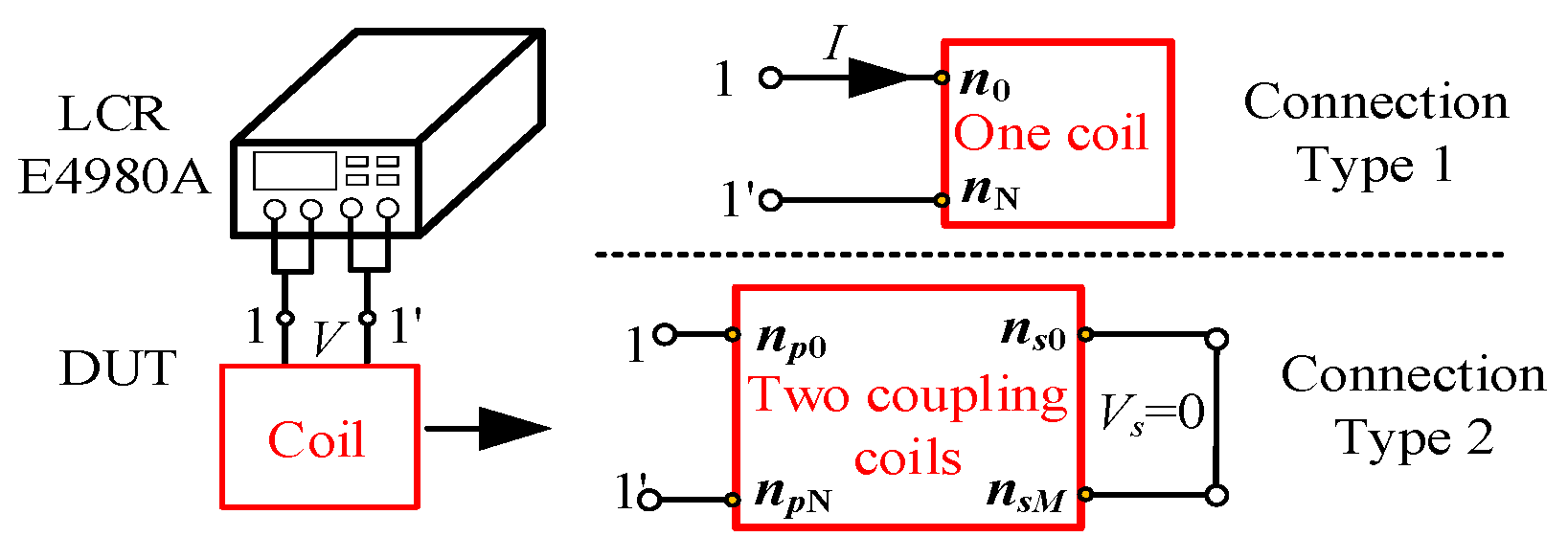
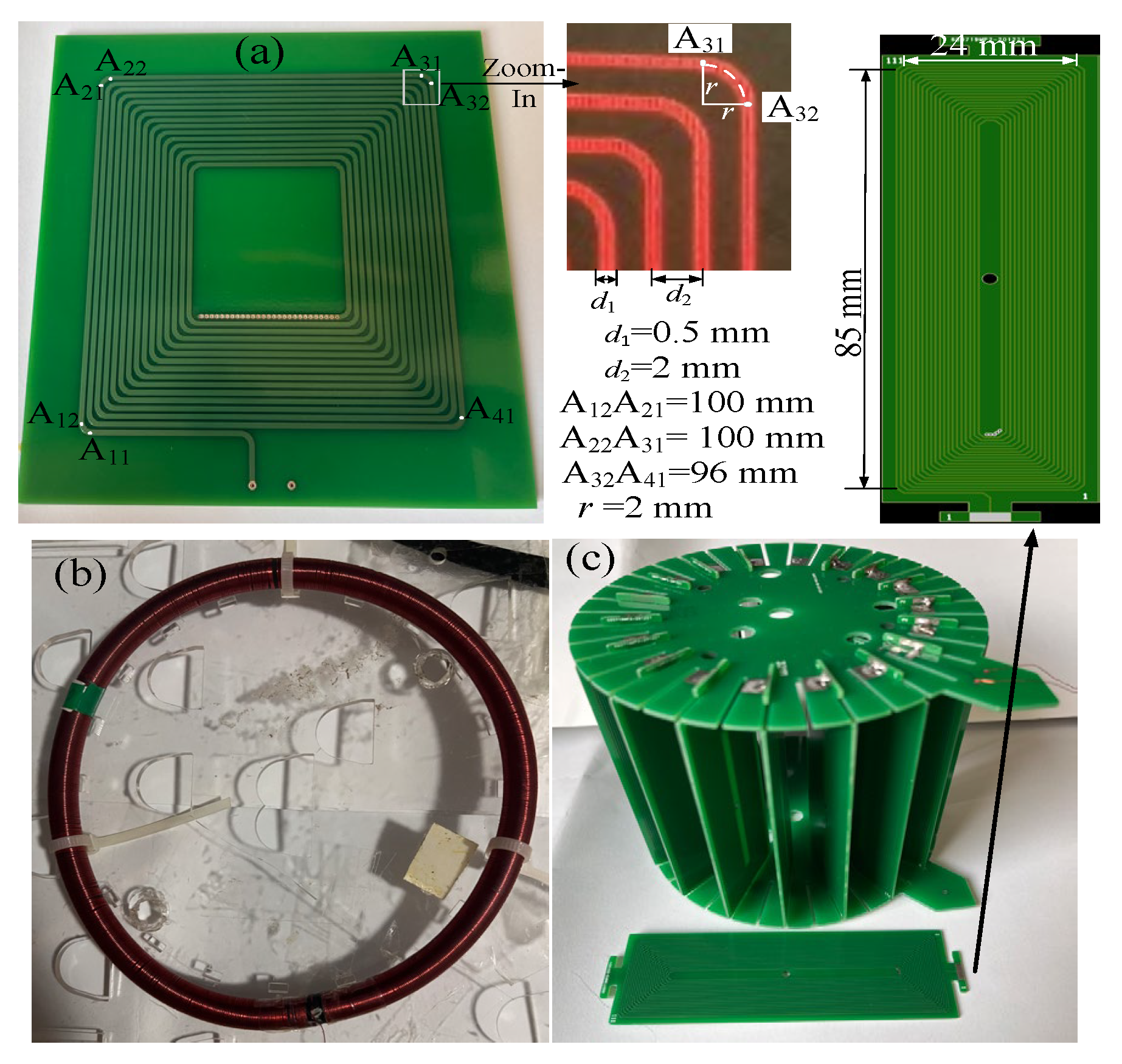
To verify the theoretical derivation, as shown in Figure 7 and Figure 8, four common types of coils with complex structures are manufactured. These coils include multilayer PCB coils, two coupled PCB coils (the relative permittivity is 4.8, and the thickness of the PCB board is 1.6 mm), a PCB coil with a complex spatial structure, and wound coils with a circular flexible frame (the radius of the circular frame is 64 mm and the cross-section radius is 3.5 mm) and 1600 turns. All the wound coils in the experiments use dense and thin windings (less than 0.2 mm). The cross-section size of the winding and the skeleton of the tested coil differ greatly (more than 1000 times). These coils are hard to model with electromagnetic simulation software. Additionally, since their structures of these coils are irregular, traditional calculation equations are also not applicable. Moreover, the coupling between the coils is also considered in the experiments. Three common circuit connections for the coils are simulated in the experiments, as shown in Figure 7. Connection type 1 simulates the case in which a multilayer coil does not have any coupling to other coils. In contrast, the type 2 connection simulates the case where the transmitting coil and the repeating coil are in a wireless transmission system. The coils are relatively close, so the capacitance between the coils is considered in the experiments.

Figure 7 shows the most common types of coils with complex structures and dense thin windings. These coils include a four-layer flat PCB coil (as shown in Figure 8a), a coil with a circular frame and 1600 turns (as shown in Figure 8b), and a PCB coil with a complex structure (as shown in Figure 8c). Some coil sizes are marked on Figure 8. The complex PCB coil is composed of 18 small PCBs and upper and lower PCB bases that fix and electrically connect the 18 PCBs. Additionally, each of the 18 small PCBs has two layers, and each layer has 20 turns (the distance between two adjacent turns is 0.508 mm, and the width of PCB wire is 0.254 mm). Four multilayer flat PCB coils, a circular coil with hundreds of 1600 turns, and the PCB coil with the complex structure are tested according to connection type 1. Conversely, a two-layer PCB coil and a two-layer short-circuit PCB coil are tested according to connection type 2. An LCR analyzer (Agilent E4980A, America Keysight, Santa Clara, CA, USA, with a maximum frequency of 2 MHz) was used to test the input impedance in the frequency range of 1 kHz~2 MHz.

3.2. Analysis of the Experimental Results and the Calculated Results

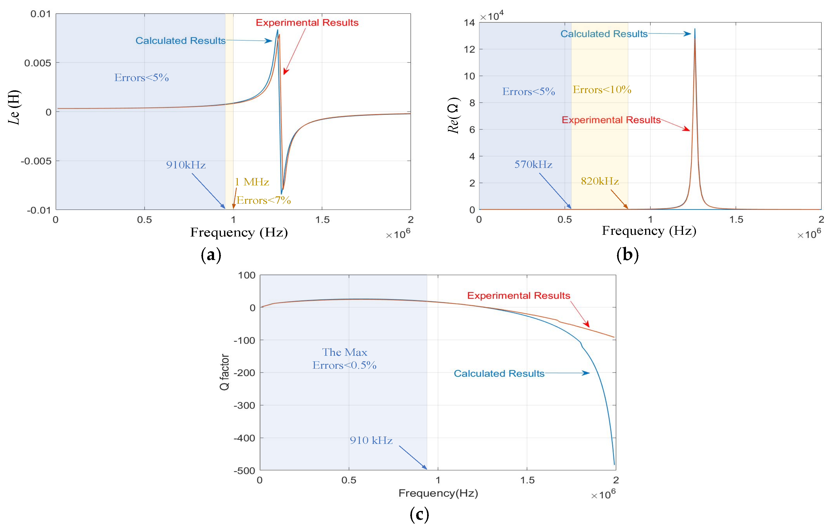
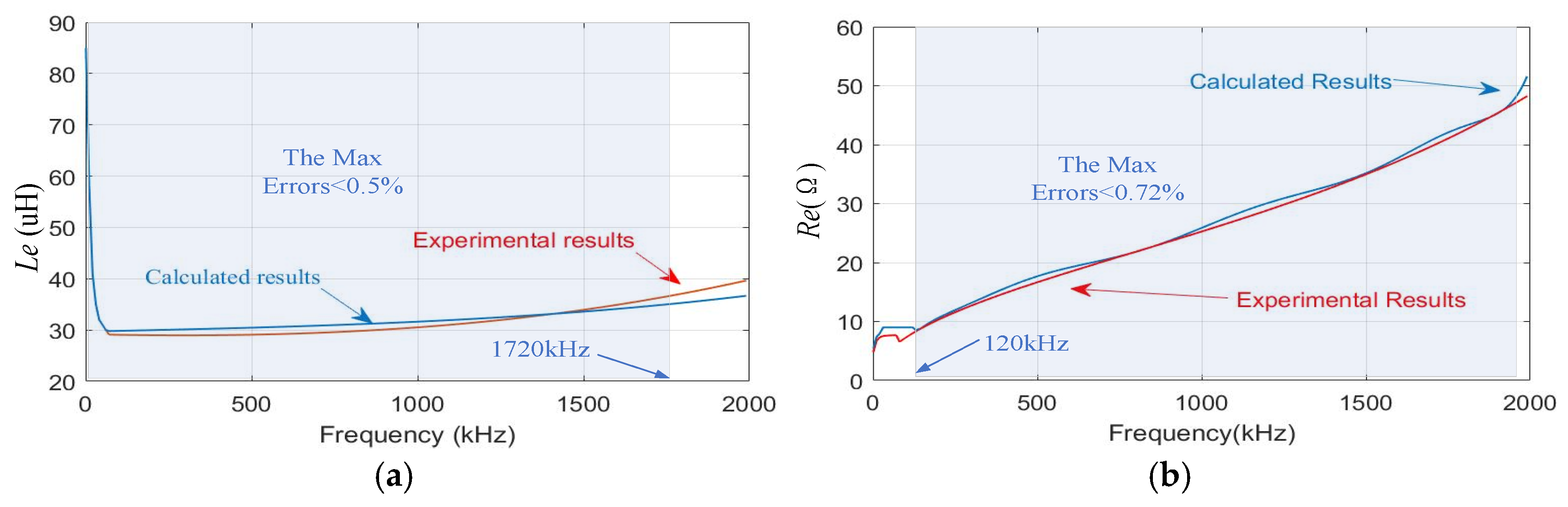
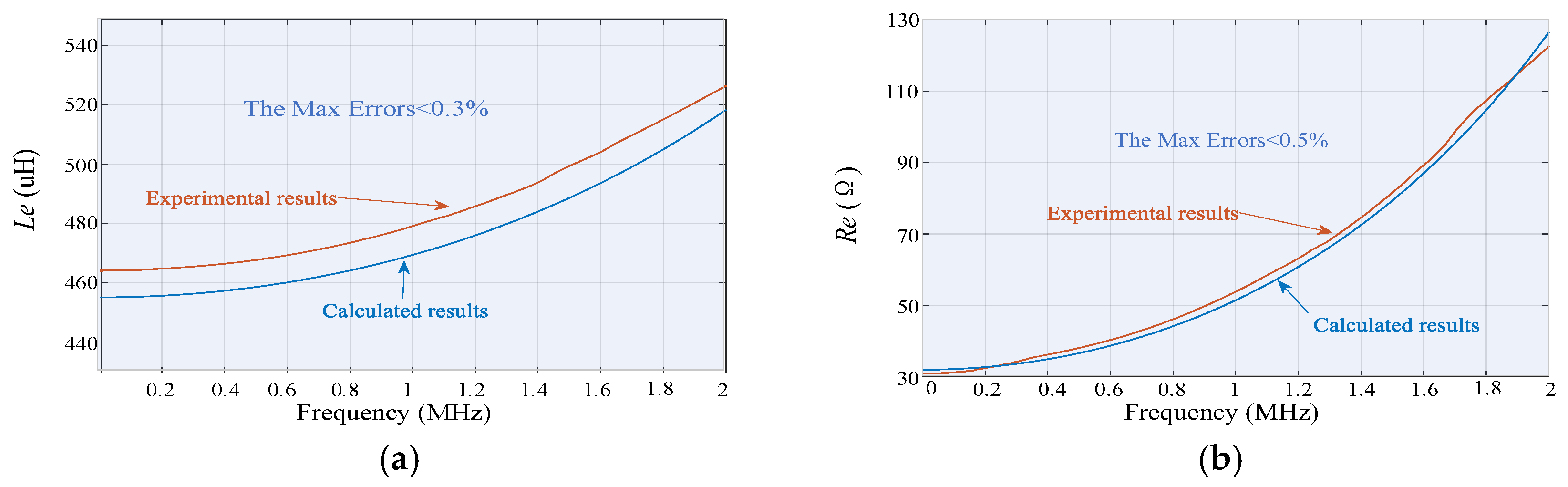
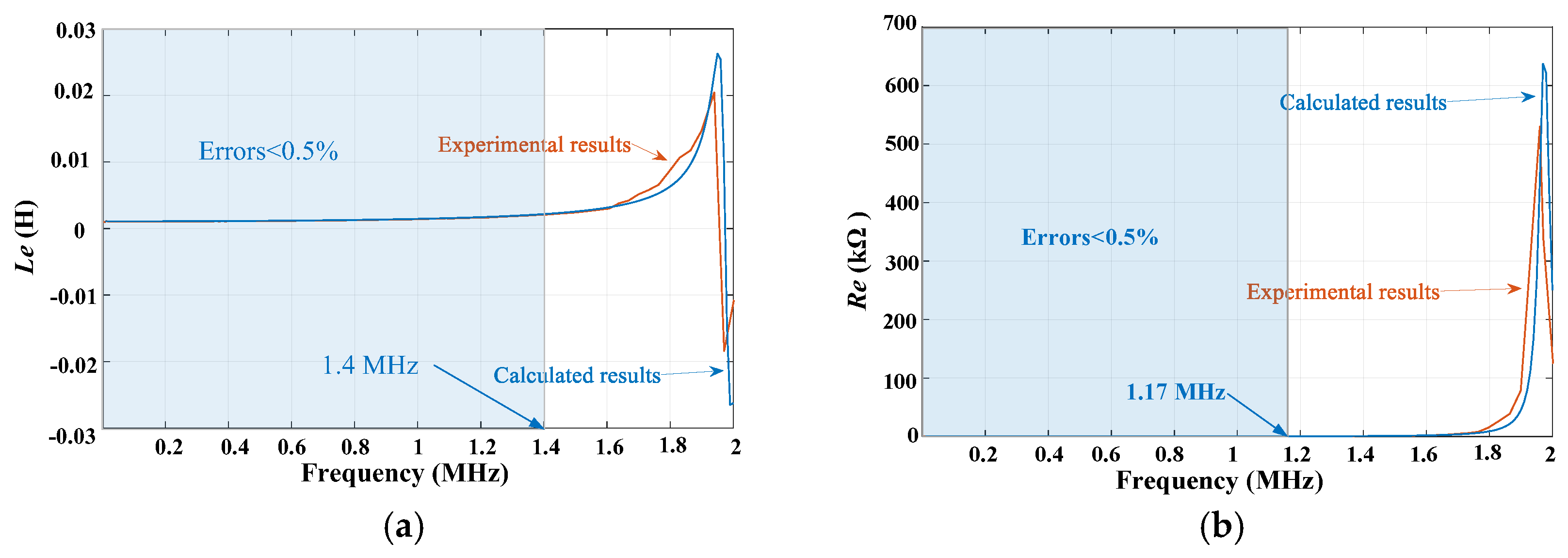
The input impedance Z_pp is taken as an example to verify the method. Figure 9, Figure 10, Figure 11 and Figure 12 shows the comparison of the experimental results and the numerical results calculated by MATLAB R2024a. By referring to the relevant materials, we set the parasitic capacitance of the probe fixture of the LCR as 5 pF. Figure 9 shows the input impedance and Q-factor of four-layer PCB coil A (connection type 1), while Figure 10 shows the input impedance of a two-layer PCB flat coil coupling with a two-layer short-circuit PCB coil (connection type 2). Figure 11 shows the input impedance of the wound coil with 1600 turns (connection type 1), and Figure 12 shows the input impedance of the PCB coil with the complex spatial structure (connection type 1). These figures show that the curves of the experimental results coincide well with the curves of the numerical results. When the frequency is not close to the resonant frequency, the error ((Experimental value − Calculated value)/Experimental value) is relatively small (less than 5%). However, when the frequency approaches the resonant frequency, this indicates that the error exceeds 5%. These errors are mainly caused by the manufacturing errors of the coils, the parameter computation methods, and the experimental process (No precise compensation or calibration were carried out for the analyzer). Thus, the closer the frequency is to the resonant frequency, the greater the influence of these external parasitic capacitance and inductance parameters.

The calculation speed of the numerical results is fast. Let us take the circular coil with 800 turns in the experiment as an example. We conducted the calculation on a laptop. The processor is intel Core i5. The running memory is 16 GB. The MATLAB version is R2017a. N1 of a turn is 100. The matrix dimensions are 800. The number of frequency points is 410, and the actual computation time is 48 min. Under the same calculation conditions, FESS is unable to divide the mesh for calculation. Both the experimental and numerical results show that the calculation method proposed in this paper can relatively accurately and quickly calculate the port frequency characteristics of the air-cored coils.

4. Conclusions

The calculation method for the electrical parameters of the hollow coils is of great importance for the design of electrical equipment and sensors. The current commonly used FESS for calculating the electrical parameters of coils is only applicable to coils with straight or segmented straight center lines along the frame. For coils with dense turns and a center line that is not straight or has an irregular shape, it is difficult to mesh the grid using the simulation software, much less calculate the electrical parameters, as the theoretical derivation is only applicable to coils with a uniform turn distribution and a regular frame shape. Therefore, there is currently no calculation method applicable to the electrical parameters of coils with irregular structure and dense turns (thousands of turns), causing difficulties for researchers.

To solve these problems, this work presents an algorithm to calculate the terminal frequency characteristics of multiple coupling coils with complex irregular structure. The hybrid calculation method proposed in this paper includes finite element simulation and theoretical derivation analytical calculation. The unit resistance parameter in this method is obtained using the ANSYS software 2022 R1, while the other calculation methods are based on analytical methods derived from theory. The skin effect, the coupling capacitance and inductance between two coil segments, and the coupling parameters between two segments of two different coupling coils are considered in this method. Although it is difficult to calculate the electrical parameters of the entire coil with dense winding and an irregular frame shape using electromagnetic simulation software, for PCB trace coils with a rectangular cross-section, the unit resistance table at different sizes and frequencies can be obtained using the two-dimensional simulation model established based on the electromagnetic simulation software and the parameter scanning and sweep frequency functions of the electromagnetic simulation software. This makes the method more accurate. The curves of the experimental results coincide well with those of the numerical result. The errors are less than 5% when the frequency is not close to the resonant frequency. The error might be partly due to the approximate calculation of the capacitance. The capacitance calculation method neglects factors such as edge fields, conductor geometry, substrate/air interface, and the interactions between multiple layers. Therefore, this method is only applicable when the frequency is not close to the resonant frequency. This method can be used to estimate the terminal characteristics of air-cored coils before manufacturing real coils with complex structure.

References

1. Xia, B.; Shen, J.X.; Luk, P.C.K.; Fei, W. Comparative study of air-cored axial-flux permanent-magnet machines with different stator winding configurations. IEEE Trans. Ind. Electron. 2015, 62, 846–856. [Google Scholar] [CrossRef] [Scilit]
2. Burchell, J.; Ahmed, N.; Mueller, M.; Galbraith, M.; Barajas-Solano, J. Project Neptune: Critical Component Tests for a Fully Flooded Direct-Drive Linear Generator for Wave Energy Convertors. In Proceedings of the 4th Asian Wave and Tidal Energy Conference, Taipei, Taiwan, 9–13 September 2018; pp. 9–13. [Google Scholar]
3. Xuan, H.V.; Thanh, H.N.; Anh, D.D. Proposed electromagnetic analytical and FEM models for the design of AFPMGs with stator ironless in wind power. In Proceedings of the 2025 Asia Meeting on Environment and Electrical Engineering (EEE-AM), Hanoi, Vietnam, 5–7 November 2025; pp. 1–7. [Google Scholar]
4. Conway, J.T. Inductance Calculations for Circular Coils of Rectangular Cross Section and Parallel Axes Using Bessel and Struve Functions. IEEE Trans. Magn. 2010, 46, 75–81. [Google Scholar] [CrossRef] [Scilit]
5. van Deursen, A.P.J.; Smulders, H.W.M.; de Graaff, R.A.A. Differentiating/Integrating Measurement Setup Applied to Railway Environment. IEEE Trans. Instrum. Meas. 2006, 55, 316–326. [Google Scholar] [CrossRef]
6. Wang, K.; Ma, D.; Gao, Y.; Dou, Y.; Li, S.; Wang, J.; Sun, J. Design and measurement of three-dimensional uniform-field coils based on swarm intelligence algorithms under ferromagnetic boundaries. Measurement 2024, 233, 114753. [Google Scholar] [CrossRef] [Scilit]
7. Liu, L.; Liao, X.; Wu, M.; Fu, Z.; Xu, Z. A Three-Component Concentric Orthogonal Air-Core Coil Sensor. IEEE Sens. J. 2025, 25, 41963–41971. [Google Scholar] [CrossRef] [Scilit]
8. Tian, Y.; Lin, Y.; Tian, J.; Xiang, L. Multi-thread sensing coil design for metal object detection of wireless power transfer systems. Measurement 2021, 184, 109952. [Google Scholar] [CrossRef] [Scilit]
9. Li, J.; Liu, Z.; Cao, J.; Wan, Z. Research on FPC coils with limited turns in planar electromagnetic tomography. Measurement 2024, 241, 115741. [Google Scholar] [CrossRef] [Scilit]
10. Chen, X.; Cui, P.; Wu, H. Design of low-noise coil for magnetocardiography based on differential magnetic coupling strength. Measurement 2025, 259, 119689. [Google Scholar] [CrossRef] [Scilit]
11. Chang, C.-J.; Tai, C.-C.; Lin, F.-W.; Kuo, C.-C.; Hung, C.-M. Effects of Flexible Induction Coil Pitch on the Heating Performance of Thermotherapy Needles. IEEE Trans. Instrum. Meas. 2020, 69, 8983–8991. [Google Scholar] [CrossRef] [Scilit]
12. Li, Y.; Dou, S.; Liu, X.; Cui, P.; Yang, Z.; Li, H.; Wen, T. Low noise magnetic field compensation based on differential biplanar coils with small coil constant. Measurement 2024, 226, 11415. [Google Scholar] [CrossRef] [Scilit]
13. Pawłowicz, B.; Kamuda, K.; Skoczylas, M.; Jankowski-Mihułowicz, P.; Węglarski, M.; Laskowski, G. Identification Efficiency in Dynamic UHF RFID Anticollision Systems with Textile Electronic Tags. Energies 2023, 16, 2626. [Google Scholar] [CrossRef] [Scilit]
14. Tomczyk, K.; Gibas, M.; Kozień, M.S. Analysis of the Dynamic Properties of the Rogowski Coil to Improve the Accuracy in Power and Electromechanical Systems. Energies 2025, 18, 4761. [Google Scholar] [CrossRef] [Scilit]
15. Lyu, G.; Ali, H.; Tan, H.; Peng, L.; Ding, X. Review on Short-Circuit Protection Methods for SiC MOSFETs. Energies 2024, 17, 4523. [Google Scholar] [CrossRef] [Scilit]
16. Gutierrez, H.; Meinke, R.; Fernando, T.; Kirk, D. Non-Contact DC Electromagnetic Propulsion by Multipole Transversal Field: Numerical and Experimental Validation. IEEE Trans. Magn. 2016, 52, 1–10. [Google Scholar] [CrossRef] [Scilit]
17. Xu, P.; Zhu, C.; Zeng, H.; Wang, P. Rail crack detection and evaluation at high speed based on differential ECT system. Measurement 2020, 166, 108152. [Google Scholar] [CrossRef] [Scilit]
18. Wang, S.; Lu, J.; Lu, F.; Lu, C.; Zhang, X. Optimal Design of Planar Coils with Reverse Current Distribution for Atomic Devices. IEEE Trans. Instrum. Meas. 2022, 71, 9006309. [Google Scholar] [CrossRef] [Scilit]
19. He, Z.; Chen, W.; Chen, X.; Tian, J. An Optimized Variable Number of Windings Approach to Design a Birdcage-Like Shift Coil for MPI System. IEEE Sens. J. 2024, 24, 18968–18976. [Google Scholar] [CrossRef] [Scilit]
20. Naseem, H.; Seok, J.-K. Wireless Charging Technologies for Electric Vehicles: Topologies, Control Strategies, Challenges, and Future Trends. Energies 2026, 19, 3531. [Google Scholar] [CrossRef] [Scilit]
21. Palka, R. Fast Analytic–Numerical Algorithms for Calculating Mutual and Self-Inductances of Air Coils. Energies 2024, 17, 325. [Google Scholar] [CrossRef] [Scilit]
22. Yang, W.; Meng, F.; Zhai, G. Collaborative Optimization of Dynamic Characteristics and Armature Structural Safety in Electromagnetic Repulsion Mechanisms. Energies 2026, 19, 3665. [Google Scholar] [CrossRef] [Scilit]
23. Venikar, P.A.; Ballal, M.S.; Umre, B.S.; Suryawanshi, H.M. Search Coil Based Online Diagnostics of Transformer Internal Faults. IEEE Trans. Power Del. 2017, 32, 2520–2529. [Google Scholar] [CrossRef] [Scilit]
24. Vasić, D.; Bilas, V.; Ambruš, D. Validation of a Coil Impedance Model for Simultaneous Measurement of Electromagnetic Properties and Inner Diameter of a Conductive Tube. IEEE Trans. Instrum. Meas. 2006, 55, 337–342. [Google Scholar] [CrossRef] [Scilit]
25. Zierhofer, C.M.; Hochmair, E.S. Geometric Approach for Coupling Enhancement of Magnetically Coupled Coils. IEEE Trans. Biomed. Eng. 1996, 43, 708–714. [Google Scholar] [CrossRef] [Scilit] [PubMed]
26. Vyroubal, D. Impedance of the Eddy-Current Displacement Probe: The Transformer Model. IEEE Trans. Instrum. Meas. 2004, 53, 384–391. [Google Scholar] [CrossRef]
27. Su, Y.P.; Liu, X.; Ron Hui, S.Y. Mutual Inductance Calculation of Movable Planar Coils on Parallel Surfaces. IEEE Trans. Power Electron. 2009, 24, 1115–1124. [Google Scholar] [CrossRef] [Scilit]
28. Crotti, G.; Giordano, D. Evaluation of Frequency Behavior of Coils for Reference Magnetic Field Generation. IEEE Trans. Instrum. Meas. 2005, 54, 718–721. [Google Scholar] [CrossRef]
29. Nakane, H. Calculation of the Difference in Impedance for a Solenoid Coil with and without a Sample Conductor. IEEE Trans. Instrum. Meas. 1991, 40, 544–548. [Google Scholar] [CrossRef] [Scilit]
30. Theodoulidis, T.; Ditchburn, R.J. Mutual Impedance of Cylindrical Coils at an Arbitrary Position and Orientation Above a Planar Conductor. IEEE Trans. Magn. 2007, 43, 3368–3370. [Google Scholar] [CrossRef] [Scilit]
31. Ali, A.; Saraereh, O.; Ware, A. Novel Design of Conical-Shaped Wireless Charger for Unmanned Aerial Vehicles. Energies 2025, 18, 5015. [Google Scholar] [CrossRef] [Scilit]
32. Bilicz, S.; Badics, Z.; Gyimóthy, S.; Pávó, J. A Full-Wave Integral Equation Method Including Accurate Wide-Frequency-Band Wire Models for WPT Coils. IEEE Trans. Magn. 2018, 54, 7203404. [Google Scholar] [CrossRef] [Scilit]
33. Zhang, Y.; Zhao, Z.; Chen, K. Frequency-Splitting Analysis of Four-Coil Resonant Wireless Power Transfer. IEEE Trans. Ind. Appl. 2014, 50, 2436–2445. [Google Scholar] [CrossRef] [Scilit]
34. Li, Z.; Wang, G.; Li, S.; Lan, J.; Han, B.; Lu, Y.; Zhang, Z.; He, Q. Mutual Inductance Measurement of the Superconducting Coil for the Joule Balance. IEEE Trans. Instrum. Meas. 2013, 62, 1531–1536. [Google Scholar] [CrossRef] [Scilit]
35. Jameson, N.J.; Azarian, M.H.; Pecht, M. Impedance-Based Condition Monitoring for Insulation Systems Used in Low-Voltage Electromagnetic Coils. IEEE Trans. Ind. Electron. 2017, 64, 3748–3757. [Google Scholar] [CrossRef] [Scilit]
36. Gomes, R.C.M.; Vitorino, M.A.; Acevedo-Bueno, D.A.; Corrêa, M.B.d.R. Multiphase Resonant Inverter with Coupled Coils for AC–AC Induction Heating Application. IEEE Trans. Ind. Appl. 2020, 56, 551–560. [Google Scholar] [CrossRef]
37. Kanaltarov, P.L.; Zeitlin, L.A. Inductance Calculation Manual, 1st ed.; China Machine Press: Beijing, China, 1992. [Google Scholar]
38. Dubickas, V.; Edin, H. High-frequency model of the Rogowski coil with a small number of turns. IEEE Trans. Instrum. Meas. 2007, 56, 2284–2288. [Google Scholar] [CrossRef] [Scilit]
Figure 1. The air-cored coils on the market. (a) Two coupled coils in the IPT system; (b) the poly-cyclic coil for measuring current; (c) the coil for measuring the current in the electrical power system; (d) the rotating dipole.
Applsci 16 09352 g001
Figure 2. Diagram of a coil with an irregular shape.
Applsci 16 09352 g002
Figure 3. Diagram and equivalent circuit of a coil. (a) wound coils; (b) the equivalent circuit.
Applsci 16 09352 g003
Figure 4. Schematic diagram of the PCB coil with a complex structure.
Applsci 16 09352 g004
Figure 5. Schematic diagram of two coupled coils with a complex structure.
Applsci 16 09352 g005
Figure 6. Two-port network of the two coupled coils.
Applsci 16 09352 g006
Figure 7. Schematic diagram of the experiments.
Applsci 16 09352 g007
Figure 8. Schematic diagram of the tested coils. (a) The multilayer PCB coil; (b) the wound coil; (c) the PCB coil with a complex structure.
Applsci 16 09352 g008
Figure 9. The input impedance of the four-layer PCB coil (connection type 1). (a) Inductance; (b) resistance; (c) Q-factor.
Applsci 16 09352 g009
Figure 10. The input impedance of two coupled coils (connection type 2). (a) Inductance; (b) resistance.
Applsci 16 09352 g010
Figure 11. The input impedance of the flexible wound coil with 1600 turns and a circular frame (connection mode 1). (a) Inductance; (b) resistance.
Applsci 16 09352 g011
Figure 12. The input impedance of the PCB coil with the complex spatial structure (connection type 1). (a) Inductance; (b) resistance.
Applsci 16 09352 g012
Disclaimer/Publisher’s Note: The statements, opinions and data contained in all publications are solely those of the individual author(s) and contributor(s) and not of MDPI and/or the editor(s). MDPI and/or the editor(s) disclaim responsibility for any injury to people or property resulting from any ideas, methods, instructions or products referred to in the content.