Deep Learning for Surface-Conditioned Structural Crack Recognition: Integrating CNN-Attention Models and Calibrated Confidence Estimation

Abstract

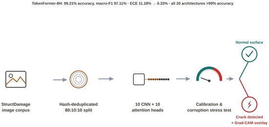
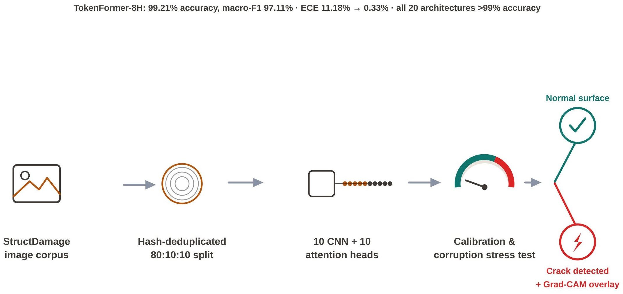
Surface recognition can organize structural inspection imagery, but high classification accuracy does not establish crack detection or structural diagnosis. This study evaluates the supplied 49,124-image StructDamage collection, containing nine surface categories and 4586 masonry-focused images. A shared ResNet-18 encoder supports ten convolutional and ten attention-based residual heads under fixed training and validation rules. The validation-selected TokenFormer-8H achieves 99.21% test accuracy and 97.11% macro-F1 on 4926 images. Temperature scaling reduces negative log-likelihood from 0.145 to 0.040 and expected calibration error from 11.18% to 0.33%. However, four selected heads retain zero residual correction, and the macro-F1 improvement over the linear control has a paired 95% component-bootstrap interval spanning zero. A revision audit identifies 101 within-class equal-perceptual-hash groups crossing partitions despite zero exact-hash overlap; excluding affected test components retains 4819 images and 99.19% accuracy. Source-folder labels alone predict 97.97% of test labels, demonstrating strong source–category confounding. A separate ImageNet-only source-held-out probe reaches 83.29% accuracy across 21 eligible folders representing three categories, without establishing nine-class external validity. Additional calibration comparisons, acquisition perturbations, and quantitative attribution tests expose class-dependent uncertainty and sensitivity to image degradation. Blur reduces macro-F1 to 46.81%, and Grad-CAM deletion does not outperform random-pixel deletion. These results support a reproducible surface-category benchmark and an audit of its limitations, not validated crack geometry, mechanism, dimensional measurement, or field safety assessment.

1. Introduction

The integrity assessment of civil infrastructure is an important component of broader structural health monitoring (SHM) and asset-management frameworks. Although sensor-based SHM systems can provide information on global or local structural response, visual inspection remains one of the principal means of identifying surface deterioration in buildings, bridges, pavements, tunnels, masonry structures, and other engineering assets [1]. Among the visible forms of deterioration encountered in structural inspection, cracking is particularly important because its occurrence, spatial distribution, and progression can provide early evidence of material degradation and developing structural distress [2,3]. If cracks remain undetected or are inadequately characterized, deterioration may progress through initiation, propagation, and unstable fracture stages, with implications for subsequent condition assessment and maintenance intervention [4]. Therefore, timely and reliable automated recognition of crack-related structural imagery is important for scalable inspection and data-driven infrastructure management [5]. Traditional structural condition assessment relies heavily on manual visual surveys, photographic documentation, and expert interpretation, processes that are time-consuming, labor-intensive, and potentially subjective when applied to extensive or difficult-to-access infrastructure [6,7]. Three-dimensional sensing and point-cloud processing have consequently emerged as complementary approaches for detecting structural surface defects and representing their spatial geometry [8]. Photogrammetric reconstruction and image-to-three-dimensional measurement techniques can further provide quantitative representations of crack geometry and surface condition [9,10]. In contrast, ordinary optical photography provides high-resolution, texture-rich information at comparatively low acquisition cost, making it attractive for automated inspection. However, structural photographs are inherently heterogeneous because illumination, shadows, surface texture, construction joints, staining, contamination, acquisition angle, background objects, and material-specific patterns can resemble or obscure actual defects [11]. Beyond image-based inspection, data-driven SHM has also developed around vibration, acoustic, strain, displacement, temperature, and other sensing modalities [12]. These characteristics make reliable recognition across heterogeneous structural-image repositories substantially more challenging than classification within a narrowly controlled laboratory dataset. Recent developments in deep learning, particularly convolutional neural networks (CNNs) [13] and Transformer or attention-based architectures [14,15], have substantially expanded the capabilities of automated structural-image analysis. Deep-learning models have been investigated for pavement and other ground-surface cracking [16,17,18], tunnel-surface inspection [19], and underwater and concrete infrastructure applications [20,21]. Nevertheless, a model developed within one material, acquisition system, or structural domain does not necessarily retain the same behavior when exposed to images collected from different sources. Concrete, asphalt, masonry, stone, tile, road surfaces, and bridge components exhibit fundamentally different textures and contextual features. Consequently, very high aggregate classification accuracy may partly reflect material or acquisition-domain separability rather than geometric crack morphology alone. This distinction is particularly important when the available labels describe surface or dataset categories rather than expert-defined crack orientation, severity, cause, or structural mechanism.

Image classification, object detection, and segmentation require different ground truth and support different interpretations. Zhuang et al. [22] studied image-level post-earthquake damage recognition, whereas Liu et al. [23] addressed mine-belt defects, an adjacent industrial application rather than civil-structure validation. Pixel-wise crack studies [24,25] and quantitative sensing or rock-image analyses [26,27] address more localized information. In directly relevant bridge work, Ruggieri et al. [28] investigated attention-enhanced detection of reinforced-concrete defects. Cardellicchio et al. [29] developed a framework combining overlapping inspection images, crack localization and segmentation, and pattern characterization. These studies evaluate defect instances or crack patterns; the present labels instead identify the surface category of a whole image. Their detection and geometry outcomes cannot be compared directly with our nine-class accuracy.

The availability and composition of representative training data remain major constraints on reliable structural-image recognition. Synthetic-data generation and augmentation have therefore been investigated as strategies for expanding structural-damage datasets and improving representation diversity when real annotated samples are limited [30,31]. Related work has also demonstrated that pretrained CNN representations can be adapted to crack-recognition applications through transfer learning and fine-tuning, reducing the need to learn all visual features exclusively from a task-specific dataset [32]. In parallel, class imbalance has become an important concern in multi-class structural-damage recognition because dominant categories can disproportionately influence training while minority defects remain poorly represented. Aung et al. [33], for example, developed a class-targeted augmentation framework for imbalanced multi-class structural damage data and demonstrated substantial improvements in minority-class performance relative to unbalanced training. However, much of the existing literature remains centered on optimizing an individual architecture, detection mechanism, or task-specific training strategy [34], making direct comparison across studies difficult. Differences in dataset composition, class prevalence, image resolution, preprocessing, augmentation, partitioning strategy, optimization schedule, model-selection criteria, and evaluation metrics can obscure whether reported improvements originate from the architecture itself or from the surrounding experimental protocol. Recent structural-damage frameworks have improved multi-task crack recognition and quantitative measurement [5] and addressed severe class imbalance through targeted data-generation strategies [33], while cross-domain transfer frameworks have been introduced to improve model performance when crack-recognition systems are transferred from source datasets to previously unseen field conditions [35]. These developments address important portions of the broader problem, but a controlled evaluation in which convolutional and attention-based recognition mechanisms operate on the same learned representation, data partitions, optimization protocol, and evaluation criteria remains valuable for establishing a defensible comparative baseline.

Beyond architecture design, reliable behavior under changing environmental and acquisition conditions has become an equally important consideration for automated structural inspection. Fan et al. [36] demonstrated this issue using real bridge crack-monitoring data affected by temperature-driven variations, showing that deep-learning performance depends on appropriate treatment of environmental effects and data representation across different bridge cases. The broader importance of representation and architecture selection has also been demonstrated in SHM using acoustic-emission signals, where Cui et al. [37] reported that the performance of KAN-based recurrent architectures varied according to both network structure and signal-segmentation configuration. These findings reinforce an important methodological point for structural-image recognition: high aggregate accuracy alone is insufficient evidence of reliable classification. Evaluation should account for class imbalance, preserve independence between training and final evaluation data, quantify uncertainty in predicted probabilities, and examine whether performance remains stable under realistic image degradation.

The present contribution is a controlled, conditional benchmark and an explicit audit of what its high scores can and cannot establish. It does not introduce a new backbone, attention mechanism, or crack-morphology detector. We use all 49,124 images in the supplied original-image collection associated with StructDamage [38], rather than claiming to reproduce every image or split in the larger published release. Twenty residual-head configurations share one learned representation, permitting comparison of small corrections to a common linear classifier. New revision analyses examine imperfect duplicate grouping, source–category confounding, class-dependent calibration, and attribution faithfulness. The contributions are:

• A traceable 49,124-image audit with the original 39,296/4902/4926 train/validation/test split, an explicit correction to the perceptual-hash isolation claim, and a 4819-image hash-isolated sensitivity analysis. Source-folder controls and a separate source-held-out linear probe quantify important limits to generalization.
• A matched comparison of ten CNN and ten attention-based residual-head configurations on one frozen ResNet-18 encoder, including an explicit linear control and identification of four selected zero-correction heads. Conclusions concern this representation and budget, not twenty independently trained end-to-end architectures.
• Validation-fitted confidence calibration evaluated with class-balanced discrimination, NLL, Brier score, ECE, class-conditional diagnostics, and additional balanced-temperature and regularized-vector comparisons. Test outcomes are not used to replace the originally validation-selected head.
• Paired component-bootstrap uncertainty, repeated head-training seeds, complete-test image-quality stress tests, quantitative Grad-CAM deletion analysis, and traceable real-image examples. Revision analyses are identified as post hoc and retain unfavorable outcomes as well as favorable ones.

The operational task is assigning an image to brick, cob, concrete, decks, pavements, road, stone, tile, or walls. This could support repository organization or preliminary routing to a specialist inspection workflow, but such downstream utility is not validated here. The task does not determine whether an image contains a crack, distinguish joints from cracks, segment a crack, or infer orientation, width, mechanism, severity, or structural reliability. In the title, surface-conditioned structural crack recognition refers to this surface-category task within a crack-image collection; category accuracy is not crack-detection accuracy.

2. Materials and Methods

The original experiment comprises corpus partitioning, common-encoder training, matched residual-head training, and validation-fitted calibration. The original split and checkpoints are retained for comparability. This revision adds retrospective diagnostic analyses without changing the selected model or promoting a head using its test rank. Original results and new post-hoc checks are distinguished throughout; neither a folder-based split nor hash isolation establishes independent field-site validation. This distinction complements the broader emphasis on acquisition variation and validation in structural monitoring [39,40,41,42].

2.1. Structural Image Corpus, Taxonomy, and Integrity Control

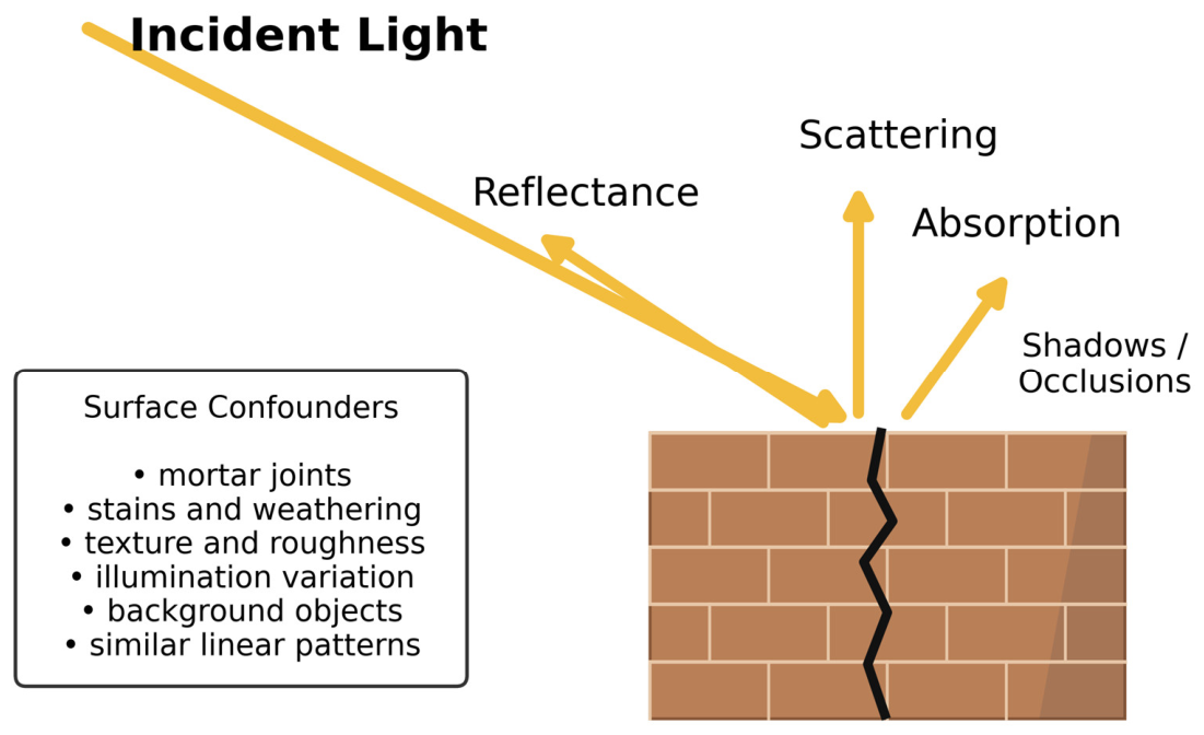
The nine labels describe surface or source-associated image categories, not crack morphology. All 49,124 JPEG/PNG files in the supplied original collection are represented in the manifest. The StructDamage source article describes a larger assembled release [38]; the scope here is the supplied original-image subset, not an assertion that 49,124 is the full published release. The separate 41,756-image balanced derivative is not an independent external cohort and is not added to the original collection as new observations. File sizes and SHA-256 hashes are rechecked against the original manifest in this revision. Heterogeneous source composition remains relevant even when files are technically valid [43,44]. The structural surface image formation and crack-confounder mechanisms is shown in Figure 1.

2.1.1. Corpus Hierarchy

Let the complete image corpus be denoted by D. It is the union of nine category-specific subsets:

$$D=\underset{c=1}{\bigcup ^9}{D}_c, \left|D\right|=\mathrm{49,124}$$

(1)

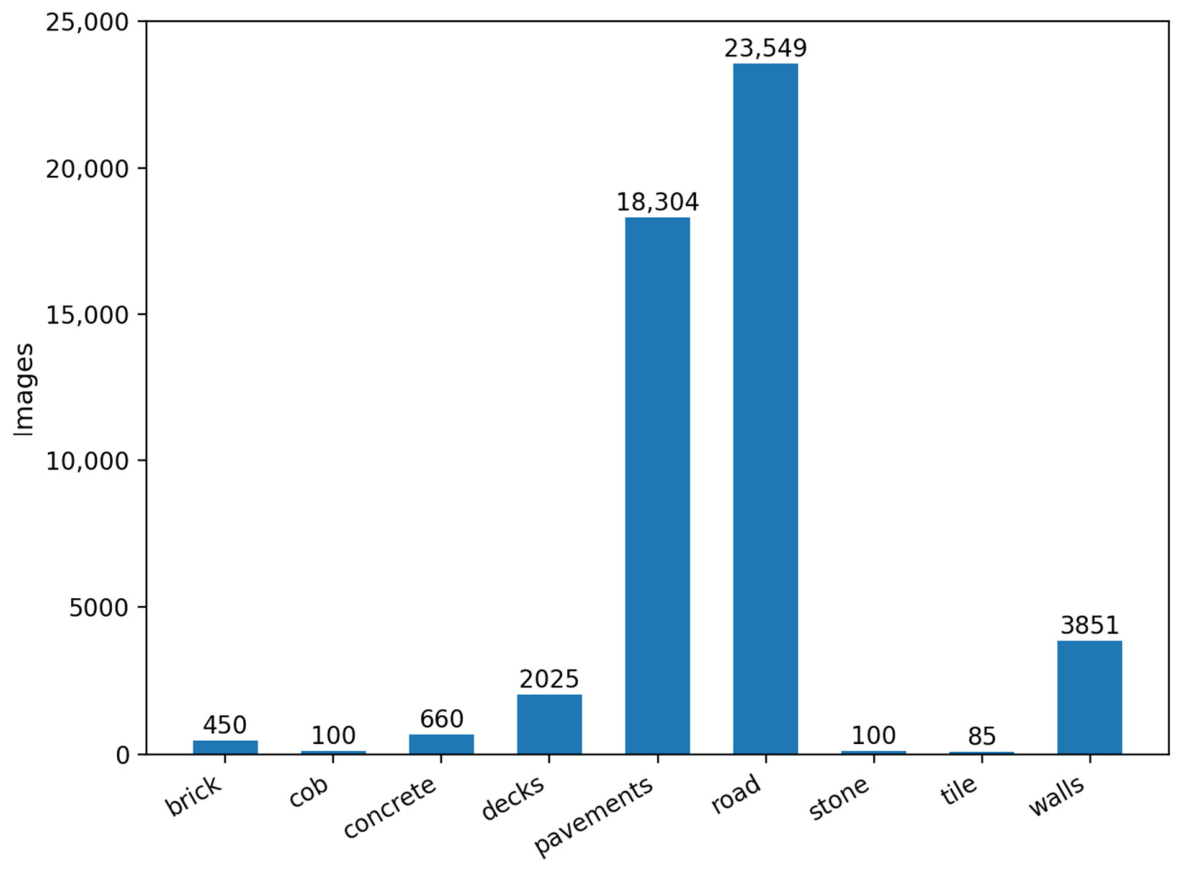
The category counts are brick (450), cob (100), concrete (660), decks (2025), pavements (18,304), road (23,549), stone (100), tile (85), and walls (3851). For reporting continuity with masonry-focused inspection, the masonry subset is defined as

$$D_{\mathrm{m}\mathrm{a}\mathrm{s}}=D_{\mathrm{b}\mathrm{r}\mathrm{i}\mathrm{c}\mathrm{k}}\cup D_{\mathrm{c}\mathrm{o}\mathrm{b}}\cup D_{\mathrm{s}\mathrm{t}\mathrm{o}\mathrm{n}\mathrm{e}}\cup D_{\mathrm{t}\mathrm{i}\mathrm{l}\mathrm{e}}\cup D_{\mathrm{w}\mathrm{a}\mathrm{l}\mathrm{l}\mathrm{s}}, \left|D_{\mathrm{m}\mathrm{a}\mathrm{s}}\right|=4586$$

(2)

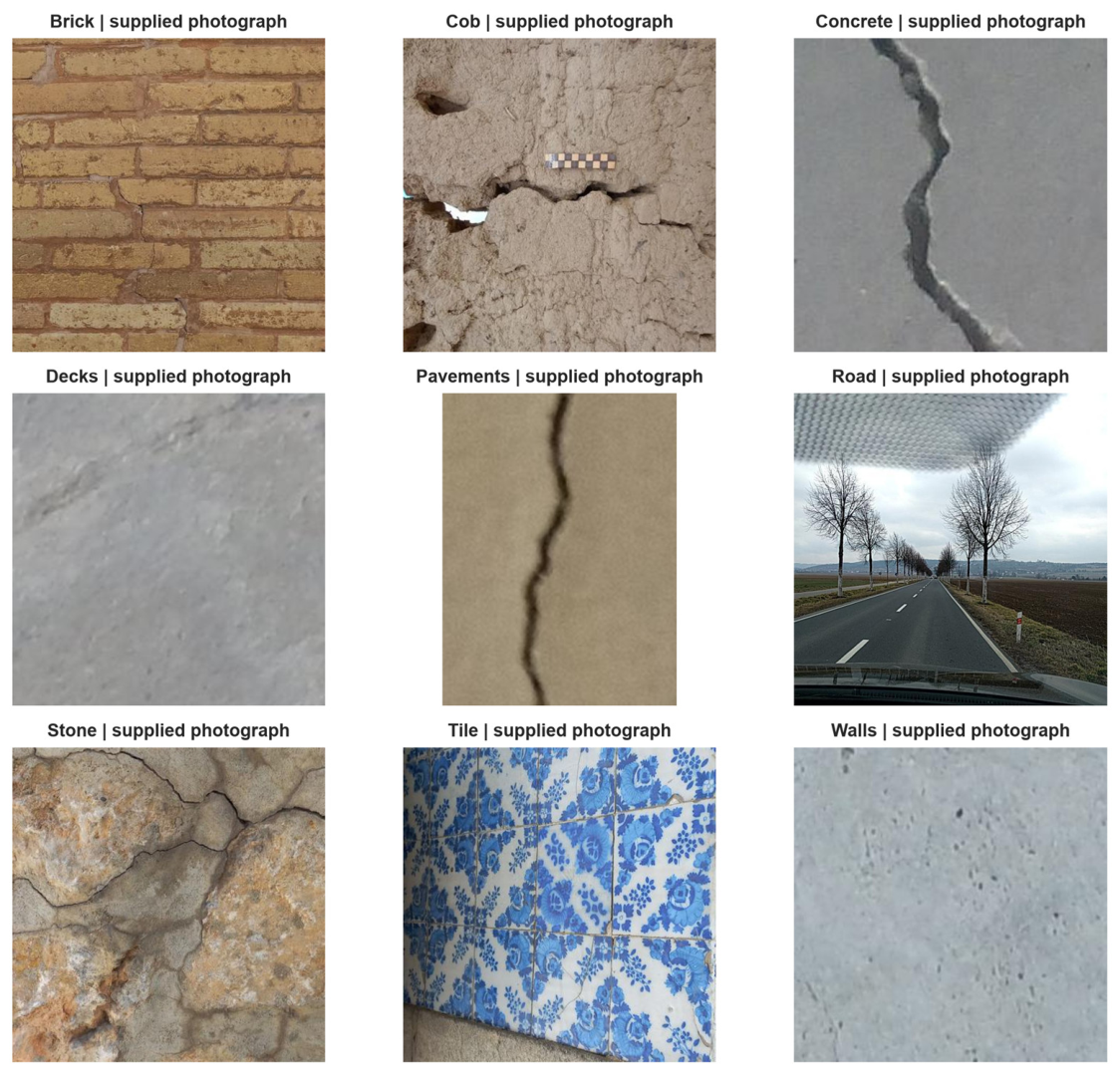
The taxonomy contains no verified crack/no-crack or construction-joint targets, masks, bounding boxes, pixel-to-millimeter scale, crack mechanism, orientation, element coordinates, stress state, or severity. Both supplied ZIP archives and the nested 155-image RAR were inspected for additional annotation files; none supplying these variables was found. The five-category masonry-focused subset is an operational grouping for continuity, and the generic walls label does not independently verify masonry construction. The original class counts and fixed train/validation/test partition is shown in

Table 1. Original class counts and fixed train/validation/test partition.

Category	All	Training	Validation	Test	Masonry Focus
brick	450	360	45	45	Yes
cob	100	80	10	10	Yes
concrete	660	528	66	66	No
decks	2025	1621	202	202	No
pavements	18,304	14,657	1809	1838	No
road	23,549	18,820	2367	2362	No
stone	100	80	10	10	Yes
tile	85	69	8	8	Yes
walls	3851	3081	385	385	Yes

. The actual test photographs representing the nine supplied surface categories is shown in Figure 2 and the natural class distribution of the complete structural-image corpus is shown in Figure 3.

2.1.2. Exact and Perceptual Duplicate Grouping

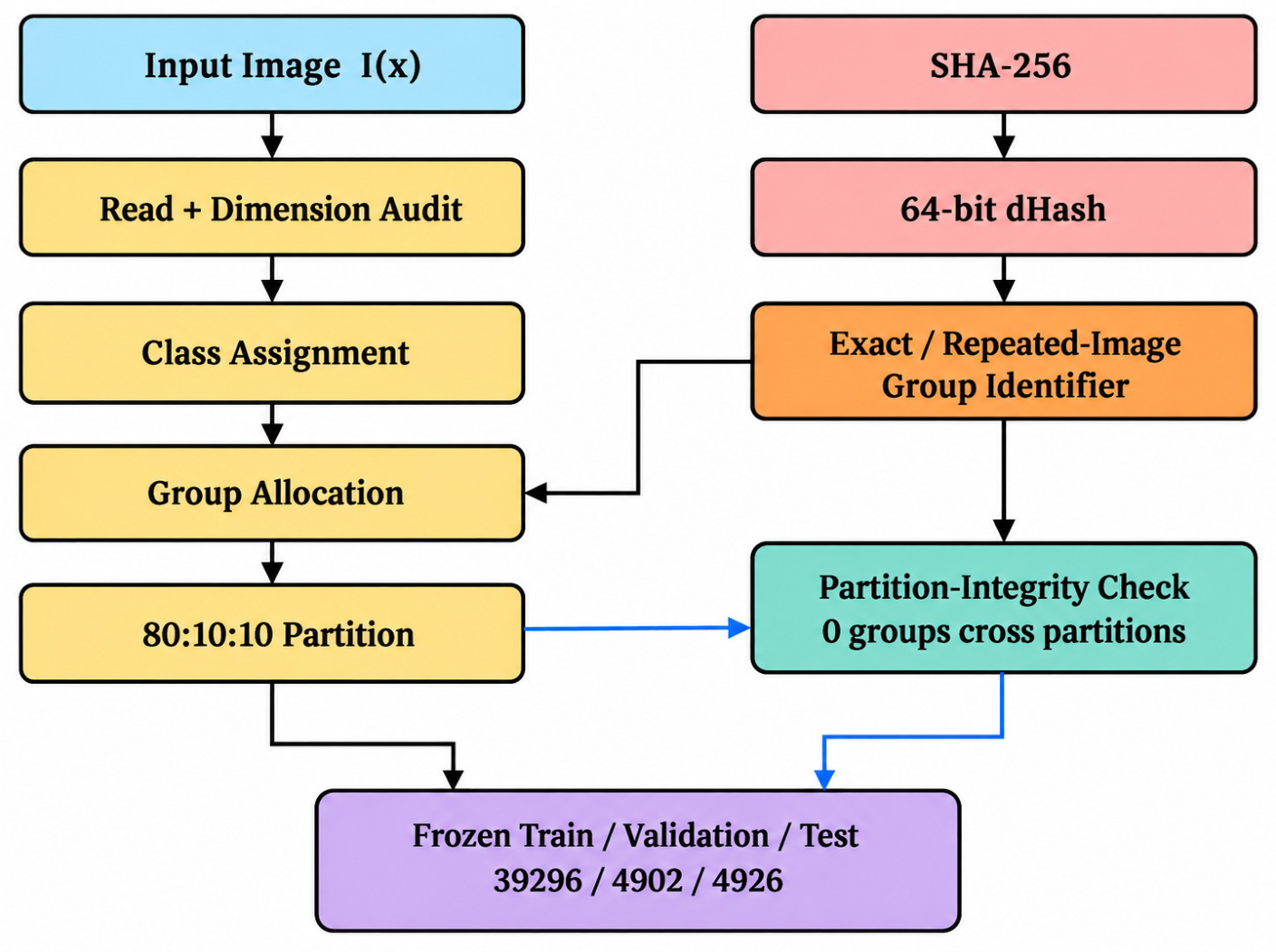
The original implementation assigns an exact SHA-256 group whenever a file has an exact duplicate; otherwise, it assigns a class-specific identical-dHash group. This precedence rule, represented schematically in Equation (3), does not combine both relationships transitively. It prevents exact-hash overlap in the stored split but can separate visually matching files when only one belongs to an exact-duplicate group. The revision therefore reconstructs connected components using the union of equal SHA-256 and within-class equal 64-bit dHash, and reports both the original grouping and the corrected audit. Equal dHash is a screening relation, not proof of identical scene content; unequal dHash does not rule out near duplication.

$$g_i=G \left(h_i^{\mathrm{S}\mathrm{H}\mathrm{A}256},\hspace{0.17em}{h}_i^{\mathrm{d}\mathrm{H}\mathrm{a}\mathrm{s}\mathrm{h}},\hspace{0.17em}{y}_i\right)$$

(3)

where $h_i^{\mathrm{S}\mathrm{H}\mathrm{A}256}$ is the exact-content hash, $h_i^{\mathrm{d}\mathrm{H}\mathrm{a}\mathrm{s}\mathrm{h}}$ is the perceptual hash, and $y_i$ is the surface-category label. The audit identified 16,896 files belonging to exact-duplicate sets and 19,683 files belonging to repeated-dHash sets. No cross-class exact-hash conflicts were detected. The counts describe repeated files, not proof that every perceptual group was isolated; the corrected union audit is reported separately.

2.1.3. Grouped 80:10:10 Partition

Within each class, original group identifiers were shuffled with seed 20260903 and assigned approximately 80:10:10 by group count, producing 39,296 training, 4902 validation, and 4926 test images. Equation (4) describes disjoint stored group identifiers, not disjoint capture sites or all perceptual matches. No exact SHA-256 group crosses partitions. The corrected union audit identifies 101 within-class equal-dHash groups crossing partitions. For a conservative sensitivity analysis, every test image whose union component also occurs in training or validation is excluded, leaving 4819 images. This is a post-hoc fixed-model evaluation, not a new training split or proof that every near duplicate is removed.

$$G_{\mathrm{t}\mathrm{r}}\cap G_{\mathrm{v}\mathrm{a}\mathrm{l}}=G_{\mathrm{t}\mathrm{r}}\cap G_{\mathrm{t}\mathrm{e}}=G_{\mathrm{v}\mathrm{a}\mathrm{l}}\cap G_{\mathrm{t}\mathrm{e}}=⌀$$

(4)

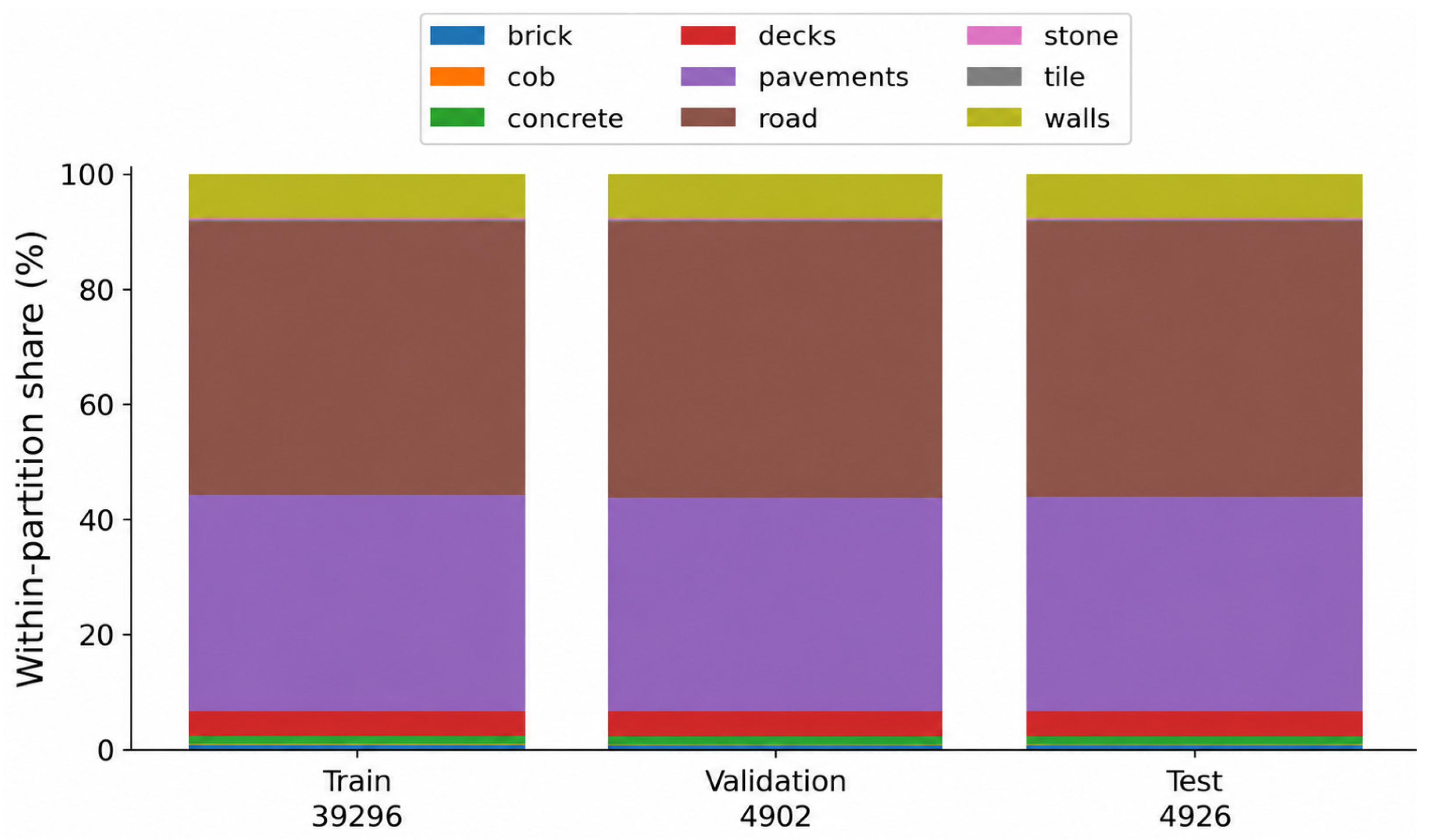
The original recorded model-selection and calibration rules use validation data. The additional hash-isolated test is reported alongside, rather than replacing, the original results. Figure 4 shows the original grouping pathway, with the corrected audit distinguished in its caption and

Table 2. Original corpus audit and partition counts, with the corrected cross-partition interpretation.

Audit Item	Measured Value
Readable images	49,124/49,124
Classes	9
Masonry-focused images	4586
Files in exact-duplicate sets	16,896
Files in repeated dHash sets	19,683
Image width range	37–4032 px
Image height range	35–4032 px
Cross-class exact-hash conflicts	0
Stored original group IDs crossing partitions	0
Cross-partition exact SHA-256 groups	0
Cross-partition within-class equal-dHash groups	101
Union-component-isolated test images	4819 (107 excluded)
Test union components for bootstrap	3920

; Figure 5 and Algorithm 1 shows the observed partition composition.

Algorithm 1 Corpus audit and duplicate-controlled partitioning

Input: Original 49,124-image corpus and supplied category labels Output: Original split plus a corrected revision integrity audit 1. Enumerate images and retain file size, SHA-256, dHash, class and source-folder string. 2. Reproduce the original grouping: exact-hash duplicates take priority; other files use class-specific equal dHash. 3. Shuffle original groups within class with seed 20260903 and allocate approximately 80:10:10. 4. Retain the original 39,296/4902/4926 split; verify zero exact-hash overlap. 5. Revision: form connected components using equal SHA-256 OR within-class equal dHash. 6. Count cross-partition matches and exclude affected test components for sensitivity analysis. 7. Preserve all original assignments and report the post-hoc status of the corrected audit.

2.2. Common Encoder and Matched Twenty-Method Recognition Benchmark

A common encoder [45] is trained once so that residual-head comparisons condition on identical features, training images, and representation quality. This reduces computational cost and one major source of experimental variation, but also limits the question being answered: which small correction, if any, improves a fixed representation under this budget? It cannot reveal which independently trained backbone or end-to-end architecture would be best. Twenty-head results must therefore be interpreted as correlated conditional experiments, not twenty independent demonstrations of crack understanding.

2.2.1. Common Representation Learning

For input image $x_i$, the encoder $f_{\theta }$ produces representation $z_i$ and common logits ${\mathsf{\ell }}_i^0$:

$$z_i=f_{\theta }\left(x_i\right), {\mathsf{\ell }}_i^0=W_0{z}_i+b_0$$

(5)

Images are resized to 96 × 96 RGB and normalized with ImageNet channel statistics. The encoder follows the recorded eight-epoch schedule, with classifier-only adaptation initially, layer 4 unfrozen from epoch 2, and layer 3 from epoch 5; the selected checkpoint is epoch 5 by validation macro-F1. Training uses batches of 128, AdamW, inverse-frequency square-root class weights, and 13,098 additional class-balanced replacement draws per epoch from epoch 2. The optimizer is recreated at each epoch in the original implementation, so its moment state is not retained between epochs. Equation (6) states the weighted, label-smoothed minibatch cross-entropy used by the implementation, with ε = 0.04 for the encoder. Weight normalization uses the sum of target-class weights in the minibatch, rather than the unweighted batch size.

$$\mathcal{L}=-{\displaystyle \frac{{\sum }_i{\sum }_c{w}_c\left[\right(1-\epsilon ) 1(c=y_i)+\epsilon /C] log p_{ic}}{{\sum }_i{w}_{y\mathrm{i}}}}$$

(6)

In Equation (6), i indexes minibatch images, c indexes the nine classes, p denotes the softmax probability, and 1(c = y_i) is the target-class indicator. The weight for class c is the square root of the total training count divided by nine times that class’s training count. Learning rates are 3 × 10⁻³ for the classifier at epoch 1; 2 × 10⁻⁴ for layer 4 and 10⁻³ for the classifier at epochs 2–4; and 7 × 10⁻⁵, 1.2 × 10⁻⁴, and 5 × 10⁻⁴ for layer 3, layer 4, and the classifier at epochs 5–8. AdamW weight decay is 2 × 10⁻⁴ and the gradient-norm limit is 3. Batch-normalization running statistics are updated in training mode, including modules whose parameters are frozen.

Encoder augmentation uses horizontal flips with probability 0.5, vertical flips with probability 0.08, independent brightness and contrast multipliers sampled uniformly from 0.85 to 1.15, and additive Gaussian noise on 35% of batches with standard deviation sampled from 0 to 0.025. Values are clipped to [0, 1] before normalization. Head training uses the fixed cached representations rather than a new independent augmentation or backbone-training experiment.

2.2.2. Residual Recognition Heads

For each head, the encoder and base classifier are frozen. The head receives the 512 × 3 × 3 layer-4 feature map and adds a gated correction to the original nine logits, as expressed in Equation (7). The gate is σ(a), with a initialized to −1.5; the correction branch ends in a zero-initialized linear layer. Only one CNN or attention adapter is active in any given model. There is no fusion ensemble of the twenty heads.

$${\mathsf{\ell }}_{\mathrm{i}}^{\left(\mathrm{m}\right)}={\mathsf{\ell }}_{\mathrm{i}}^{\left(0\right)}+\sigma \left(a_{\mathrm{m}}\right){\Delta }_{\mathrm{m}}\left(z_{\mathrm{i}}\right)$$

(7)

$$p_i^m=\mathrm{s}\mathrm{o}\mathrm{f}\mathrm{t}\mathrm{m}\mathrm{a}\mathrm{x}\left({\mathsf{\ell }}_i^m\right)$$

(8)

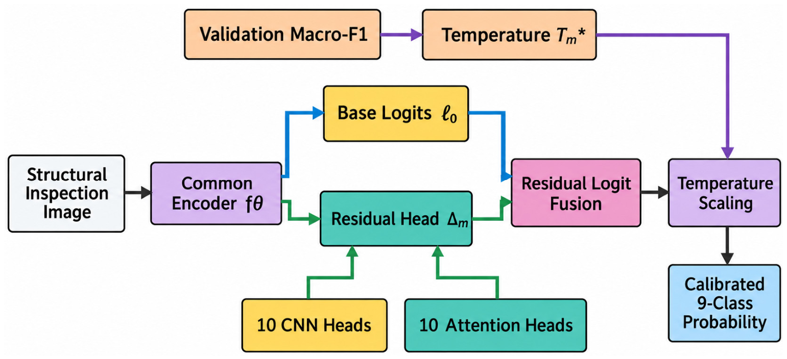
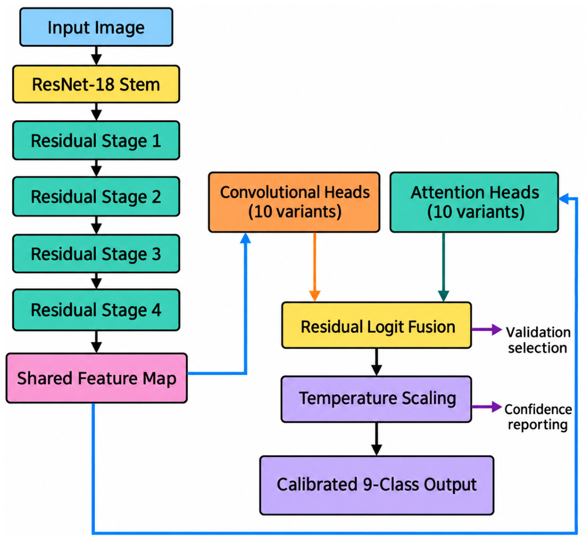
Zero initialization makes the epoch-0 prediction exactly the common linear baseline. Epoch 0 remains eligible for validation selection; consequently, SPP-Conv, Deep-TokenFormer, Class-Attention, and Pyramid-Attention retain a zero correction at their selected checkpoint. These four configurations are functional linear controls, not independently successful learned attention or convolutional models. The parameter counts in

Table 3. Twenty matched residual recognition heads.

Method	Family	Defining Operation	Trainable Parameters
Class-Attention (epoch 0)	Attention	class-query cross-attention	101,802
Cross-Covariance	Attention	channel covariance attention	101,802
Deep-TokenFormer (epoch 0)	Attention	two transformer layers	139,402
Gated-TokenMixer	Attention	depthwise token mixing + gate	101,802
Hybrid-ConvFormer	Attention	token convolution + transformer	101,802
Pyramid-Attention (epoch 0)	Attention	class/mean/max token fusion	101,802
TokenFormer-2H	Attention	one transformer layer, 2 heads	101,802
TokenFormer-4H	Attention	one transformer layer, 4 heads	101,802
TokenFormer-8H	Attention	one transformer layer, 8 heads	101,802
Window-Attention	Attention	overlapping local token windows	101,802
CBAM-CNN	CNN	channel + spatial attention	44,589
Depthwise-CNN	CNN	depthwise-separable spatial block	47,242
Dilated-CNN	CNN	dilation-2 spatial block	79,370
GAP-MLP	CNN	global average pooling + MLP	42,442
GeM-MLP	CNN	learned generalized-mean pooling	42,443
Inception-CNN	CNN	1 × 1/3 × 3/dilated branches	72,722
Pointwise-CNN	CNN	1 × 1 channel mixing	54,890
Residual-CNN	CNN	two-layer residual block	116,554
SE-CNN	CNN	squeeze-excitation gating	44,570
SPP-Conv (epoch 0)	CNN	1/2/3-level spatial pyramid	148,938

describe registered head parameters, including any registered modules unused by a selected adapter; they do not include the frozen encoder. The matched residual-head recognition and validation-only calibration framework is illustrated in Figure 6. The Common ResNet-18 encoder with alternative convolutional and attention-based recognition branches and calibrated output is illustrated in Figure 7.

2.2.3. Controlled Head Training and Validation Selection

Each head is evaluated at epoch 0 and after five training epochs. Training uses batch size 512, AdamW with learning rate 8 × 10⁻⁴ and weight decay 2 × 10⁻⁴, cosine decay to 2 × 10⁻⁵, gradient-norm clipping at 3, and label smoothing ε = 0.02 with class weighting. The original feature cache stores float16 maps, which are converted to float32 for head computation. The checkpoint maximizing validation macro-F1 is retained, and the head with the highest validation macro-F1 is selected as TokenFormer-8H. The zero-correction checkpoints are retained rather than silently discarded.

$$m^{*}=\mathrm{a}\mathrm{r}\mathrm{g}\underset{m}{\mathrm{m}\mathrm{a}\mathrm{x}}{F}_{1,\hspace{0.17em}\mathrm{m}\mathrm{a}\mathrm{c}\mathrm{r}\mathrm{o},\mathrm{v}\mathrm{a}\mathrm{l}}\left(m\right)$$

(9)

The common-encoder training and matched residual-head selection is illustrated in Algorithm 2.

Algorithm 2 Common-encoder training and matched residual-head selection

Input: Original training and validation partitions Output: Common encoder and twenty validation-selected conditional heads 1. Train the encoder under the recorded eight-epoch schedule; select by validation macro-F1. 2. Freeze the selected encoder and its original linear classifier. 3. For each CNN or attention adapter, initialize its final correction layer to zero and gate parameter to −1.5. 4. Evaluate epoch 0 and five trained epochs with the common head budget. 5. Retain each head’s best validation macro-F1 checkpoint, including epoch 0 when selected. 6. Select TokenFormer-8H by validation macro-F1; do not promote a head using test rank. 7. Record the four zero-correction selections and preserve the linear control.

2.3. Confidence Calibration, Evaluation Metrics, and Statistical Analysis

The original calibration method is scalar temperature scaling [46]. Calibration changes confidence, not the target task: a confident surface label is not a probability that a crack is present or that a structure is unsafe. The same validation partition is used for head selection and calibration fitting; it is not a separate calibration cohort.

2.3.1. Validation-Only Temperature Scaling

For method m, the fitted temperature is

$$T_m^{*}=\mathrm{a}\mathrm{r}\mathrm{g}\underset{T>0}{\mathrm{m}\mathrm{i}\mathrm{n}}\hspace{0.17em}{\mathrm{N}\mathrm{L}\mathrm{L}}_{\mathrm{v}\mathrm{a}\mathrm{l}} \left({\mathsf{\ell }}^m/T\right)$$

(10)

and calibrated class probabilities are obtained as

$${\tilde{p}}_i^m=\mathrm{s}\mathrm{o}\mathrm{f}\mathrm{t}\mathrm{m}\mathrm{a}\mathrm{x} \left({\mathsf{\ell }}_i^m/T_m^{*}\right)$$

(11)

A positive scalar temperature preserves the per-image argmax and therefore accuracy, macro-F1, and balanced accuracy. It need not preserve one-versus-rest probability rankings across different images, so macro-AUROC is recomputed after scaling. Scalar scaling cannot independently repair class-specific biases, supply epistemic uncertainty, or guarantee reliability after an acquisition shift.

2.3.2. Discrimination and Calibration Measures

The primary discrimination measures are macro-F1 and balanced accuracy. Overall accuracy, macro precision, macro recall, Matthews correlation coefficient (MCC), Cohen’s kappa, and macro area under the receiver operating characteristic curve (macro-AUROC) are reported as complementary measures. For class c, precision and recall are

$${\mathrm{P}\mathrm{r}\mathrm{e}\mathrm{c}\mathrm{i}\mathrm{s}\mathrm{i}\mathrm{o}\mathrm{n}}_c={\displaystyle \frac{T{P}_c}{T{P}_c+F{P}_c}}, {\mathrm{R}\mathrm{e}\mathrm{c}\mathrm{a}\mathrm{l}\mathrm{l}}_c={\displaystyle \frac{T{P}_c}{T{P}_c+F{N}_c}}$$

(12)

$$F_{1,\mathrm{m}\mathrm{a}\mathrm{c}\mathrm{r}\mathrm{o}}={\displaystyle \frac{1}{C}}{\displaystyle \sum _{c=1}^C}{\displaystyle \frac{2\hspace{0.17em}{\mathrm{P}\mathrm{r}\mathrm{e}\mathrm{c}\mathrm{i}\mathrm{s}\mathrm{i}\mathrm{o}\mathrm{n}}_c\hspace{0.17em}{\mathrm{R}\mathrm{e}\mathrm{c}\mathrm{a}\mathrm{l}\mathrm{l}}_c}{{\mathrm{P}\mathrm{r}\mathrm{e}\mathrm{c}\mathrm{i}\mathrm{s}\mathrm{i}\mathrm{o}\mathrm{n}}_c+{\mathrm{R}\mathrm{e}\mathrm{c}\mathrm{a}\mathrm{l}\mathrm{l}}_c}}$$

(13)

$$\mathrm{B}\mathrm{a}\mathrm{l}\mathrm{a}\mathrm{n}\mathrm{c}\mathrm{e}\mathrm{d}\hspace{0.25em}\mathrm{A}\mathrm{c}\mathrm{c}\mathrm{u}\mathrm{r}\mathrm{a}\mathrm{c}\mathrm{y}={\displaystyle \frac{1}{C}}{\displaystyle \sum _{c=1}^C}{\mathrm{R}\mathrm{e}\mathrm{c}\mathrm{a}\mathrm{l}\mathrm{l}}_c$$

(14)

Confidence quality is assessed by negative log-likelihood (NLL), multiclass Brier score, and 15-bin expected calibration error (ECE).

$$\mathrm{N}\mathrm{L}\mathrm{L}=-{\displaystyle \frac{1}{N}}\sum _i\mathrm{l}\mathrm{o}\mathrm{g}{\tilde{p}}_{i,y_i}$$

(15)

$$\mathrm{B}\mathrm{r}\mathrm{i}\mathrm{e}\mathrm{r}={\displaystyle \frac{1}{N}}\sum _i\sum _c{\left({\tilde{p}}_{ic}-y_{ic}\right)}^2$$

(16)

$$\mathrm{E}\mathrm{C}\mathrm{E}=\sum _k{\displaystyle \frac{\left|B_k\right|}{N}}\hspace{0.17em}\left|\mathrm{a}\mathrm{c}\mathrm{c}\left(B_k\right)-\mathrm{c}\mathrm{o}\mathrm{n}\mathrm{f}\left(B_k\right)\right|$$

(17)

2.3.3. Paired Statistical Testing and Bootstrap Uncertainty

The primary revision uncertainty analysis uses 5000 paired bootstrap resamples of the 3920 union-hash components represented in the original test set, sampled with replacement with seed 20260912. All images in a sampled component are retained, and identical resamples are used for every model. The 95th percentile intervals are reported for accuracy, macro-F1, balanced accuracy, and paired differences from the linear control. These intervals condition on the fixed data collection, split, and encoder; hash components are not verified across independent sites. Original image-level Cochran’s Q and Holm-adjusted exact McNemar outputs are retained as secondary descriptive checks because within-component dependence weakens their independence assumptions. Three-seed runs assess head initialization and shuffle variability with the same encoder, not full-pipeline uncertainty. Algorithm 3 illustrates the calibration, final evaluation, and paired statistical analysis.

Algorithm 3 Calibration, final evaluation, and paired statistical analysis

Input: Fixed checkpoints, validation logits and original test images Output: Calibrated predictions and conditional uncertainty estimates 1. Fit one positive temperature to each head by validation NLL; freeze it. 2. Reproduce predictions and compute class-balanced and aggregate test metrics. 3. Revision: construct union-hash components and resample the 3920 test components 5000 times. 4. Use identical resamples for all heads and the linear control. 5. Report percentile intervals for accuracy, macro-F1, balanced accuracy and paired differences. 6. Retain image-level Cochran’s Q and McNemar/Holm results only as secondary dependent-data diagnostics. 7. Fit balanced-temperature and regularized-vector alternatives on validation data; report all test outcomes without selecting a replacement. 8. Interpret repeated seeds as head-training variation with one fixed encoder.

2.4. Robustness, Visual Explanation, and Implementation Details

The original five fixed perturbations are applied to all 4926 test images: 52% brightness reduction, additive Gaussian noise with standard deviation 0.055 on [0, 1], 5 × 5 mean blur, 32 × 32 downsampling followed by nearest-neighbor upsampling, and 42% contrast reduction about the image mean. The revision adds gamma exponents 0.7 and 1.5, a left-to-right illumination multiplier from 0.35 to 1.0, RGB white-balance multipliers (1.2, 1.0, 0.8), a fixed perspective warp, and JPEG quality 30 with subsampling 2. Perspective corners (0, 0), (95, 0), (95, 95), (0, 95) map to (8, 5), (88, 0), (95, 89), (0, 95), using bilinear interpolation and filling with RGB (124, 116, 104). All six additions operate on the same cached 96 × 96 images with the original temperature fixed. They approximate selected acquisition disturbances; they do not represent newly observed cameras, weather, or inspection sites. Algorithm 4 illustrates the robustness and explanation protocol.

Algorithm 4 Robustness and explanation protocol

Input: Validation-selected model with the original temperature fixed Output: Image-quality sensitivity, attribution diagnostics and traceable examples 1. Evaluate the original five fixed corruptions on all 4926 test images. 2. Add six documented acquisition-like transformations to the same full test set. 3. Sample up to 50 component-distinct images per class without correctness selection. 4. Compute layer-3 Grad-CAM; count empty heatmaps. 5. Compare top-attribution and seeded random-pixel deletion at 10%, 20% and 30% area. 6. Bootstrap paired target-probability-drop differences over 323 component-distinct images. 7. Show actual images and traceable failures; do not claim crack-mask, physical-scale or field validation.

2.5. Reproducibility and Computational Record

The original study uses Python 3.11 and PyTorch 2.5.1+cpu. The complete computational record retains image manifests, hashes, split assignments, checkpoints, calibration values, training histories, predictions, and repeated-seed results. Revision analyses reload every original head checkpoint; all twenty class-prediction vectors reproduce the stored test predictions, with maximum probability discrepancy below 10⁻⁵. New audit tables, source-probe predictions, bootstrap samples, calibration parameters, perturbation predictions, attribution records, and figure traceability are retained separately. Original experiments and new diagnostics are not presented as one prospectively sealed analysis.

2.6. Revision-Stage Diagnostic Protocols

2.6.1. Source Controls and Hash-Isolated Evaluation

A source-only negative control maps each preserved source-folder string to its majority training class and applies that mapping to test files without image pixels. Folder strings are not verified site or device identifiers. Twenty-six of the 27 strings contain only one class, making source and label strongly entangled. The hash-isolated sensitivity analysis and component bootstrap use connected components of equal SHA-256 OR within-class equal dHash. No test labels are used to define these components.

For an additional source-held-out diagnostic, a separate ResNet-18 uses the locally available ImageNet weights without any StructDamage fine-tuning. Its 512-dimensional pooled features are extracted for all 49,124 images. Each fold holds out one complete source-folder string, removes matching union components from the remaining training pool, and fits training-only standardization followed by a class-balanced ridge classifier with fixed regularization α = 1. A fold is excluded if a held-out class has no training examples outside that folder. No fold-specific hyperparameter tuning is performed. The same probe is also fitted on the original training partition as a reference. The source-held-out probe is a different model from the submitted fine-tuned encoder and is not external field validation.

2.6.2. Additional Calibration Comparisons

Alongside raw probabilities and the original scalar temperature, a balanced temperature minimizes equal-class validation NLL, with each image weighted inversely by its validation class count. A regularized vector calibrator uses one positive scale and one centered bias per class. It minimizes mean validation NLL plus 0.01 times the sum of the mean squared deviation of scales from one and the mean squared centered biases. Log-scales and unconstrained biases are bounded to [−3, 3]; L-BFGS-B runs for at most 1000 iterations. All settings are fixed before inspecting these diagnostic test outputs. No calibrator is selected using test performance. Equal-class NLL is the unweighted mean of the nine true-class mean NLL values.

2.6.3. Quantitative Attribution and Retrospective Examples

Grad-CAM [47] is computed from the third residual stage for the predicted class. With seed 20260912, up to 50 component-distinct test images are sampled per class without conditioning on correctness, yielding 323 images. Each heatmap is bilinearly expanded to 96 × 96. The highest-attribution 10%, 20%, or 30% of pixels are replaced by the original image’s per-channel mean; a seeded random-pixel mask of equal area provides the comparator. The target is fixed to the original predicted class, and the original calibration temperature is retained. Mean target-probability drops and their paired differences are reported with 5000 image resamples; the sample contains at most one image per union component. Empty heatmaps are counted. This is a perturbation-based attribution diagnostic, not crack-mask overlap or a geometric faithfulness guarantee.

A retrospective four-image walkthrough uses existing test photographs and records manifest ID, relative path, hash, label, prediction, and calibrated confidence. Two correct brick/wall examples and the two highest-confidence test errors illustrate the actual classifier output. The selection is explicitly illustrative and cannot estimate field accuracy. No new site visit, expert structural assessment, physical scale, or crack annotation is claimed.

3. Results

Results first reproduce the original conditional benchmark and then report revision-stage integrity, source, calibration, attribution, and acquisition diagnostics. All scores refer to supplied surface categories. A test score near 99% is not a measured crack-detection sensitivity, joint false-positive rate, or structural safety accuracy.

3.1. Experimental Setup

3.1.1. Dataset Preparation

The corpus contains 49,124 images, including 4586 in the operational masonry-focused grouping. The original split is 39,296/4902/4926. Roads and pavements constitute 85.20% of the corpus and 4200 of 4926 test images. There is no exact-hash cross-partition overlap, but the stronger perceptual-isolation claim was not supported by the original precedence-based grouping. Section 3.5 reports the corrected audit and fixed-model sensitivity analysis.

3.1.2. Implementation Details

The encoder is selected at epoch 5 of the recorded eight-epoch schedule. All heads share this encoder and the same validation-selection rule. Four heads select their zero-correction epoch-0 checkpoint. Repeated-head experiments use seeds 20260903, 20260904, and 20260905 with the same representation and split. Reported reproducibility does not establish independence of capture sites or replication of full encoder training.

3.2. Evaluation Metrics

Macro-F1 and balanced accuracy are emphasized alongside aggregate accuracy. Confidence quality is evaluated with NLL, multiclass Brier score, and 15-bin ECE; equal-class mean NLL is added for the calibration comparison. The revision replaces image-resampling uncertainty as the primary interval analysis with paired hash-component resampling. Intervals reflect test-sample variation under this grouping, not all sources of model or domain uncertainty.

3.3. Comparison of Twenty Matched Recognition Methods

The common encoder achieved 99.07% test accuracy, 96.48% macro-F1, 97.18% balanced accuracy, and 0.99985 macro-AUROC. Its class-wise results in

Table 4. Original common-encoder test performance by surface category.

Category	Precision	Recall	F1	Support
Brick	1.000	1.000	1.000	45
Cob	0.800	0.800	0.800	10
Concrete	0.957	1.000	0.978	66
Decks	0.894	1.000	0.944	202
Pavements	0.998	0.987	0.993	1838
Road	0.997	0.997	0.997	2362
Stone	1.000	1.000	1.000	10
Tile	1.000	1.000	1.000	8
Walls	0.981	0.961	0.971	385

show perfect test F1 for brick, stone, and tile, while cob remained the weakest class at F1 = 0.800. The relatively small supports for cob, stone, and tile make those class-specific estimates less stable than the estimates for road, pavement, walls, and decks.

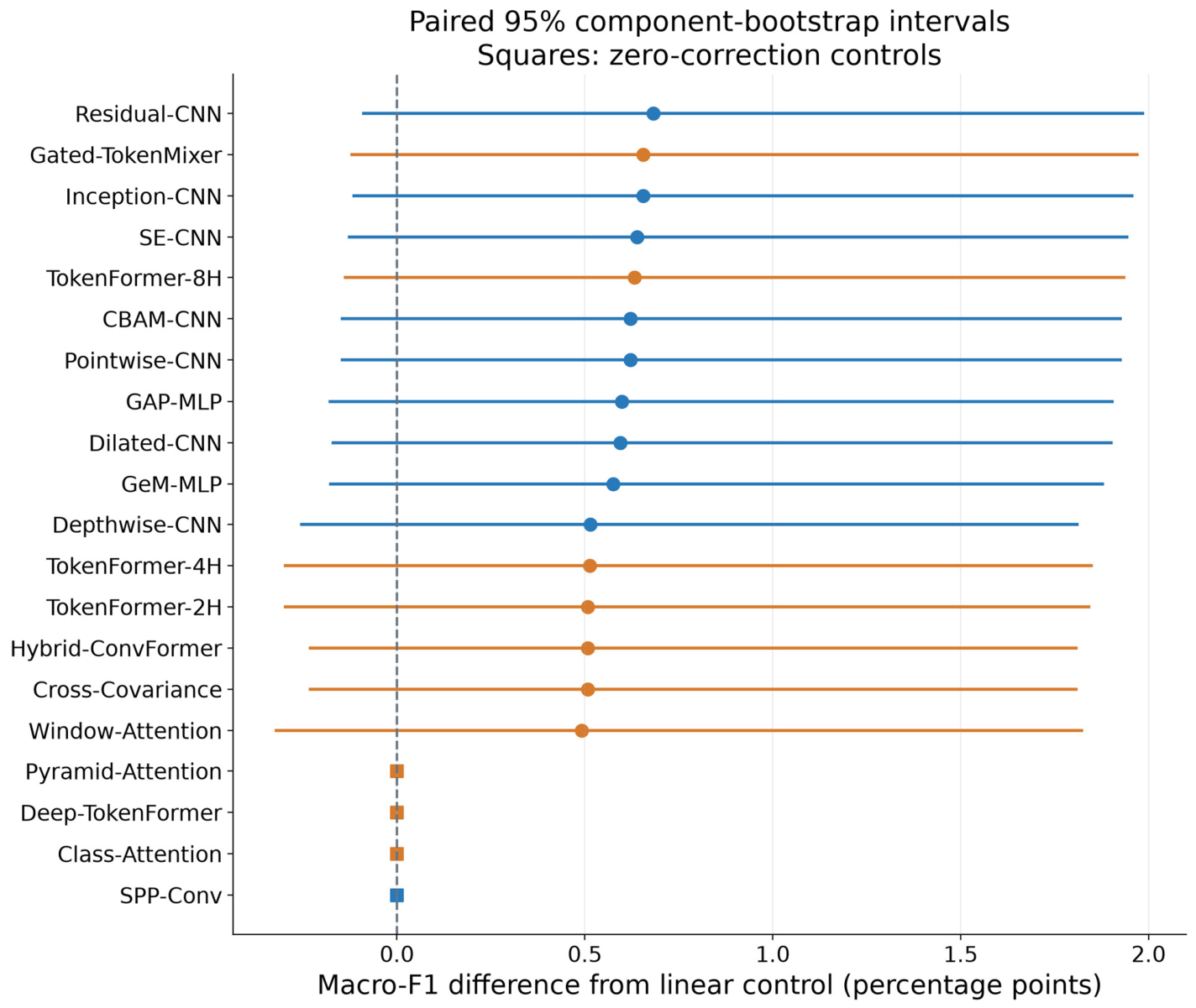
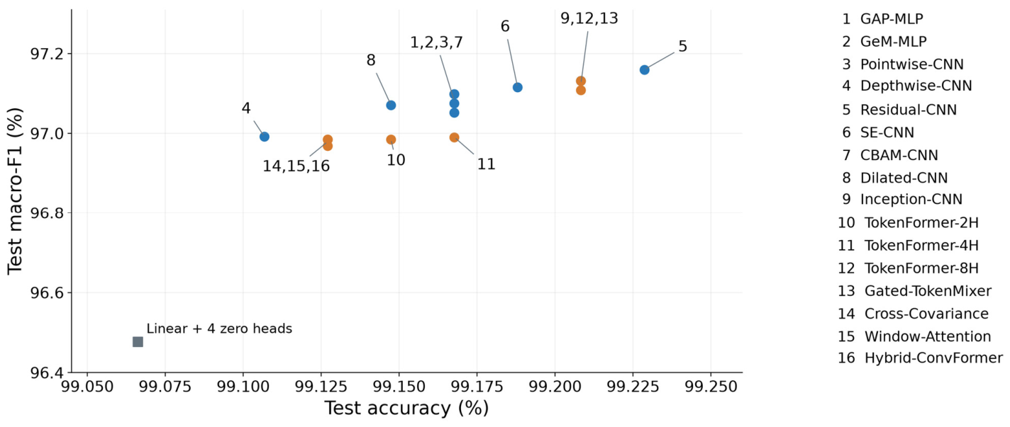
Residual-CNN has the highest observed test accuracy (99.23%) and macro-F1 (97.16%), whereas TokenFormer-8H remains the model selected by validation macro-F1 and achieves 99.21% accuracy and 97.11% macro-F1. All twenty named configurations exceed 99% accuracy, but four reproduce the linear baseline.

Table 5. Test results for twenty conditional head configurations. Rank is descriptive; the asterisk identifies the validation-selected model. Four epoch-0 heads reproduce the linear control.

Rank	Method	Family	Acc. %	Macro-F1 %	Bal. Acc. %	MCC	ECE %
1	Residual-CNN	CNN	99.23	97.16	96.90	0.988	0.42
2	Gated-TokenMixer	Attention	99.21	97.13	96.89	0.987	0.34
3	Inception-CNN	CNN	99.21	97.13	96.89	0.987	0.40
4	SE-CNN	CNN	99.19	97.12	96.89	0.987	0.36
5	TokenFormer-8H	Attention	99.21	97.11	96.87	0.987	0.33
6	Pointwise-CNN	CNN	99.17	97.10	96.88	0.987	0.42
6	CBAM-CNN	CNN	99.17	97.10	96.88	0.987	0.39
8	GAP-MLP	CNN	99.17	97.08	96.86	0.987	0.38
9	Dilated-CNN	CNN	99.15	97.07	96.88	0.986	0.41
10	GeM-MLP	CNN	99.17	97.05	96.90	0.987	0.46
11	Depthwise-CNN	CNN	99.11	96.99	96.82	0.986	0.42
12	TokenFormer-4H	Attention	99.17	96.99	96.70	0.987	0.39
13	TokenFormer-2H	Attention	99.15	96.99	96.69	0.986	0.36
14	Hybrid-ConvFormer	Attention	99.13	96.98	96.87	0.986	0.42
14	Cross-Covariance	Attention	99.13	96.98	96.87	0.986	0.44
16	Window-Attention	Attention	99.13	96.97	96.68	0.986	0.38
17	SPP-Conv	CNN	99.07	96.48	97.18	0.985	0.37
17	Deep-TokenFormer	Attention	99.07	96.48	97.18	0.985	0.37
17	Class-Attention	Attention	99.07	96.48	97.18	0.985	0.37
17	Pyramid-Attention	Attention	99.07	96.48	97.18	0.985	0.37

is a descriptive test ranking, not a basis for replacing the validation-selected model. Paired intervals in Figure 8 show that numerical ordering should not be equated with reliable architectural superiority.

The difference between Residual-CNN (97.16% macro-F1) and GAP-MLP (97.08%) is 0.08 percentage points. TokenFormer-8H improves macro-F1 over the linear control by 0.63 percentage points, but the paired 95% interval is −0.14 to 1.93 percentage points. Against Residual-CNN, its difference is −0.05 percentage points (95% interval −0.16 to 0.02). Neither interval establishes a clear macro-F1 advantage. Figure 9 retains the accuracy–macro-F1 comparison while distinguishing zero-correction controls.

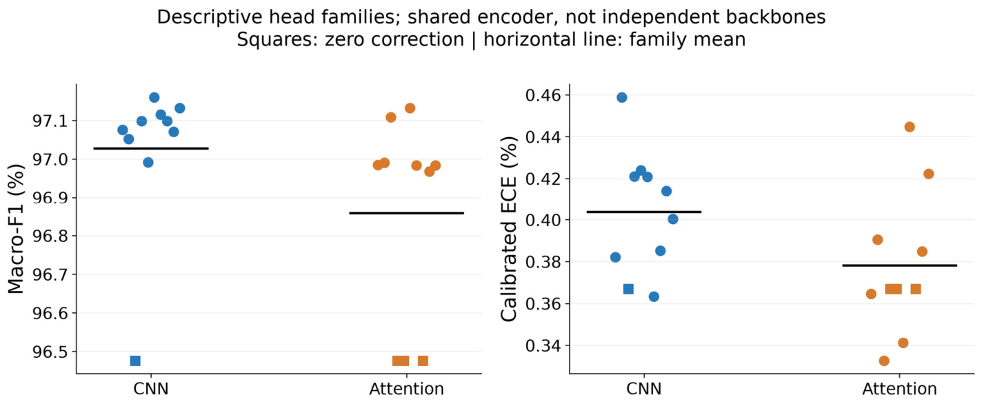
CNN heads average 97.03% macro-F1 and attention heads 96.86% in this conditional benchmark. These averages include one CNN and three attention zero-correction configurations. The observations share an encoder and test collection, and the families are not independent samples of backbone architectures. Figure 10 is descriptive only; it cannot establish general CNN superiority over transformers.

3.4. Controlled Calibration, Uncertainty, and Robustness Analysis

3.4.1. Calibration and Bootstrap Uncertainty

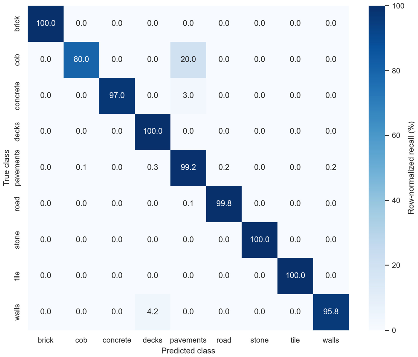
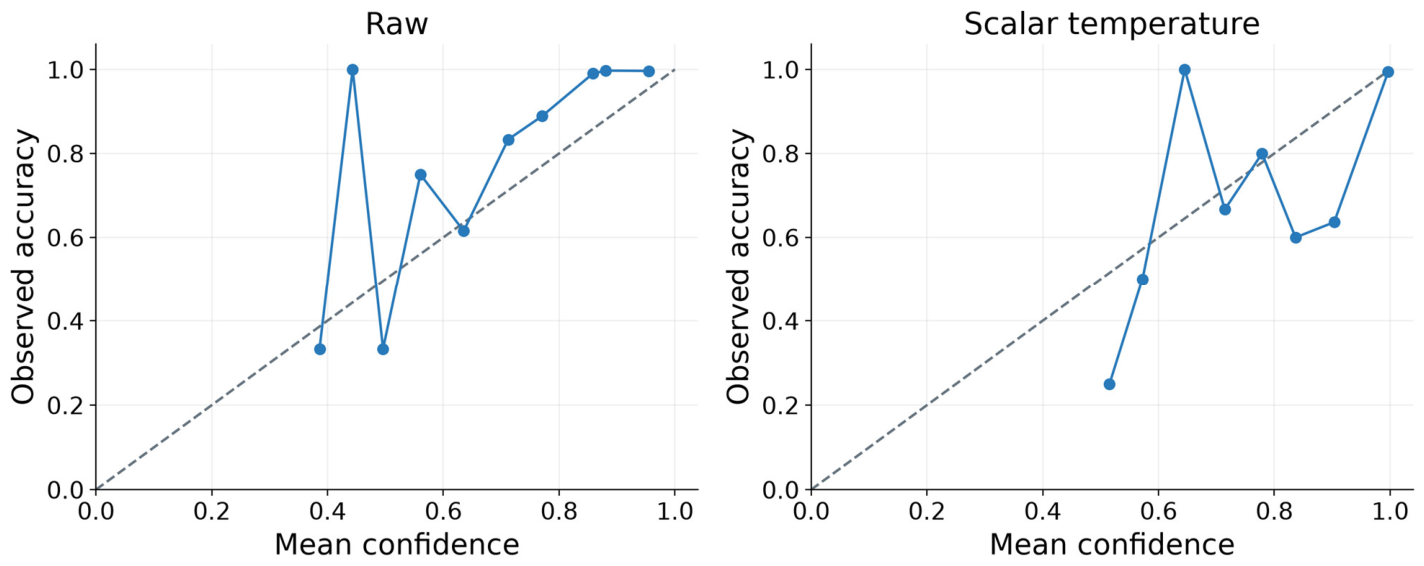
TokenFormer-8H uses validation-fitted T = 0.487. Scalar scaling reduces NLL from 0.145 to 0.040, Brier score from 0.029 to 0.014, and ECE from 11.18% to 0.33% without changing class decisions. Its accuracy is 99.21% (95% component-bootstrap interval 98.95–99.45%), macro-F1 is 97.11% (94.41–98.89%), and balanced accuracy is 96.87% (93.58–99.33%). The relatively broad class-balanced intervals reflect, in part, rare categories with only 8–10 test images. The Validation-selected TokenFormer-8H with 95% union-component bootstrap intervals is tabulated in

Table 6. Validation-selected TokenFormer-8H with 95% union-component bootstrap intervals.

Measure	Estimate	95% Component CI/Note
Accuracy	99.21%	98.95–99.45%
Macro-F1	97.11%	94.41–98.89%
Balanced accuracy	96.87%	93.58–99.33%
MCC	0.987	Not bootstrapped
Macro-AUROC	0.99980	Not bootstrapped
Calibrated ECE	0.33%	15 equal-width bins

. The row-normalized confusion matrix for the validation-selected TokenFormer-8H is illustrated in Figure 11.

The confusion matrix identifies the principal residual class errors. Cob recall was 80%, with the remaining cob cases assigned to pavements. Walls achieved 95.8% row-normalized recall, with the dominant confusion directed toward decks. Road, brick, stone, tile, and decks were nearly or completely diagonal under the observed test partition. The reliability before and after scalar temperature scaling on the same test set is illustrated in Figure 12.

3.4.2. Repeated-Seed Stability

The three leading validation-ranked heads remained tightly clustered across repeated residual-head initialization and shuffle order. TokenFormer-8H produced 99.154 ± 0.077% accuracy and 97.040 ± 0.146% macro-F1, while Gated-TokenMixer and Window-Attention showed similarly small variation. Because the common encoder and data partition were held fixed, this analysis quantifies head-level training variability rather than full-pipeline variability. The three-seed stability for the leading validation-ranked heads is tabulated in

Table 7. Three-seed stability for the leading validation-ranked heads.

Method	Family	Seeds	Accuracy %, Mean ± SD	Macro-F1 %, Mean ± SD	ECE %, Mean
TokenFormer-8H	Attention	3	99.154 ± 0.077	97.040 ± 0.146	0.371
Gated-TokenMixer	Attention	3	99.147 ± 0.054	97.039 ± 0.081	0.408
Window-Attention	Attention	3	99.141 ± 0.042	96.997 ± 0.130	0.385

.

3.4.3. Paired Statistical Comparison

The original image-level Cochran’s Q is 38.644 with 19 degrees of freedom (p = 0.0049), and exact McNemar/Holm outputs are retained in the computational record. Because images within duplicate components are not independent observations, this p-value is not used to establish practical architectural superiority. The primary paired component-bootstrap result is the uncertain 0.63-percentage-point macro-F1 increment over the linear control. No correction head is declared universally superior on the basis of these small differences.

3.4.4. Robustness and Failure Analysis

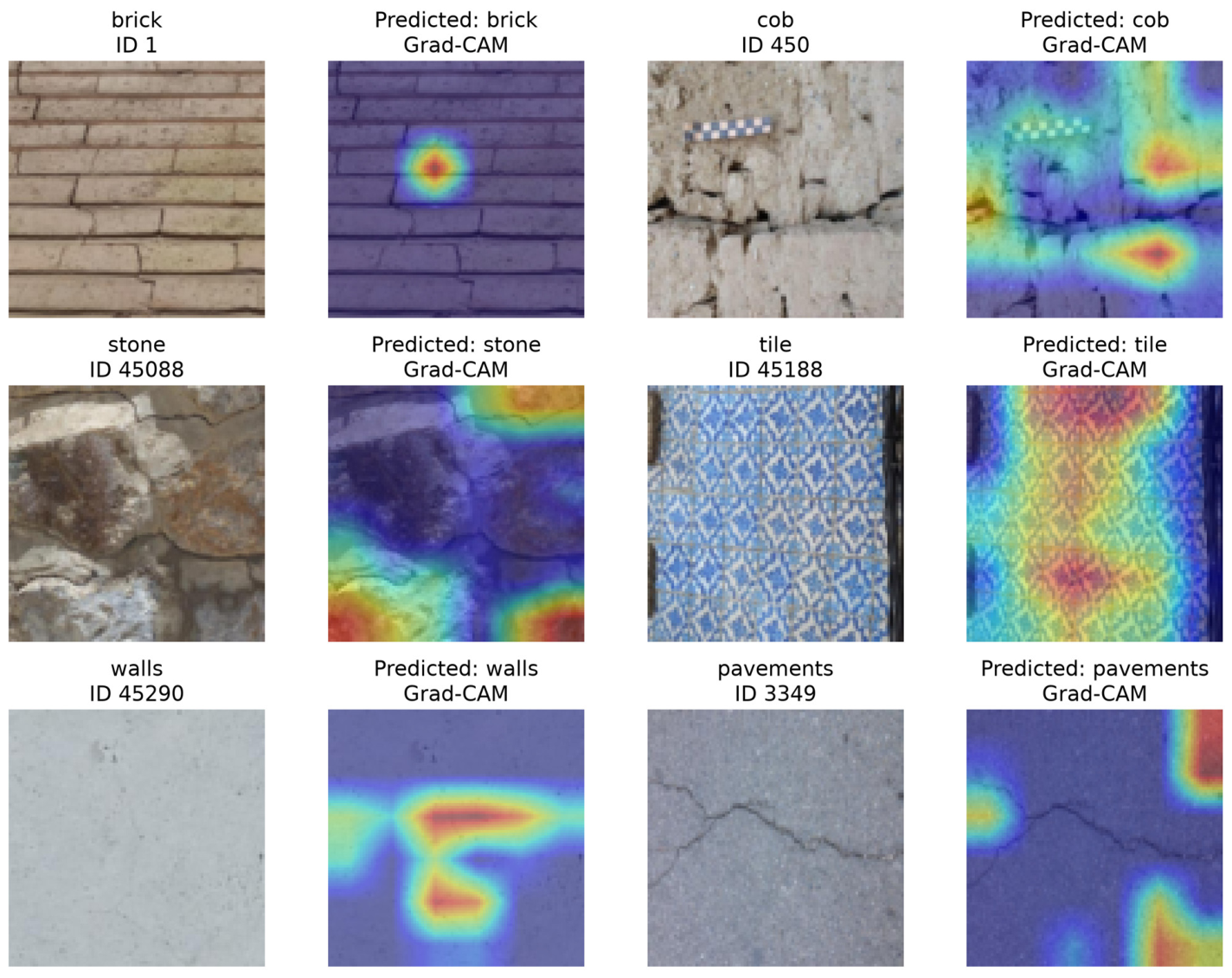
Deterministic image-quality perturbations produced a substantially wider performance range than the clean-model benchmark. Low contrast caused the smallest degradation, retaining 95.94% accuracy and 88.89% macro-F1. Pixelation retained 93.26% accuracy, while low light reduced accuracy to 92.29%. Gaussian noise reduced accuracy to 87.41%, and blur was the most severe stressor at 76.63% accuracy and 46.81% macro-F1. Calibration quality deteriorated in parallel, with ECE increasing from 0.33% on clean images to 20.18% under blur.

Table 8. Fixed-model sensitivity to the original deterministic test corruptions. Temperature is not refitted on corrupted test images.

Condition	Accuracy %	Macro-F1 %	Bal. Acc. %	ECE %	Acc. Drop pp
Clean	99.21	97.11	96.87	0.33	0.00
Low Light	92.29	78.01	74.40	6.13	6.92
Gaussian Noise	87.41	68.35	65.48	10.77	11.79
Blur	76.63	46.81	52.32	20.18	22.57
Pixelation	93.26	78.25	75.83	4.48	5.95
Low Contrast	95.94	88.89	84.57	2.32	3.27

tabulates the fixed-model sensitivity to the original deterministic test corruptions. Figure 13 illustrates the original photographs beside layer-3 Grad-CAM overlays for six cases from the component-distinct attribution sample.

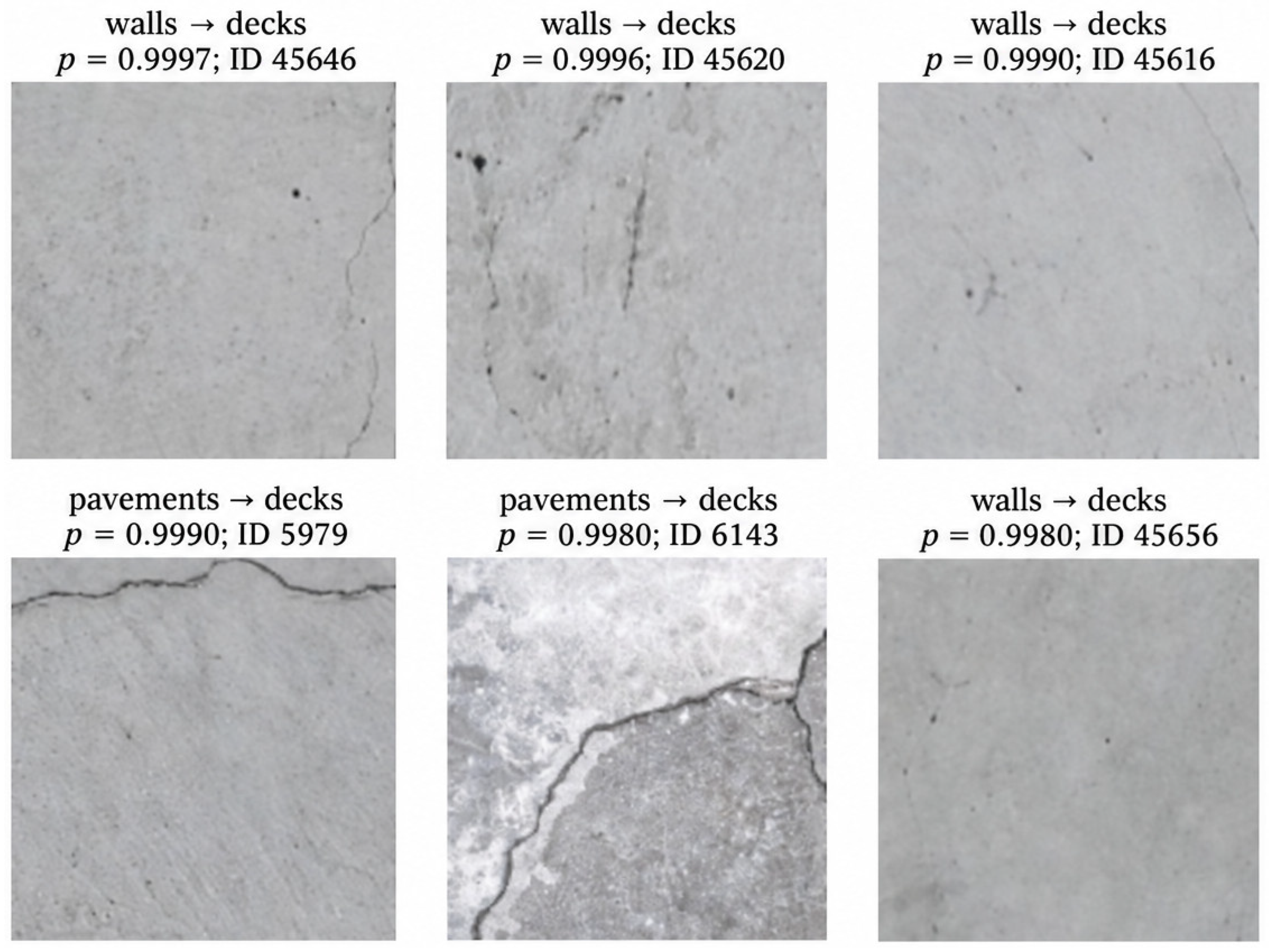
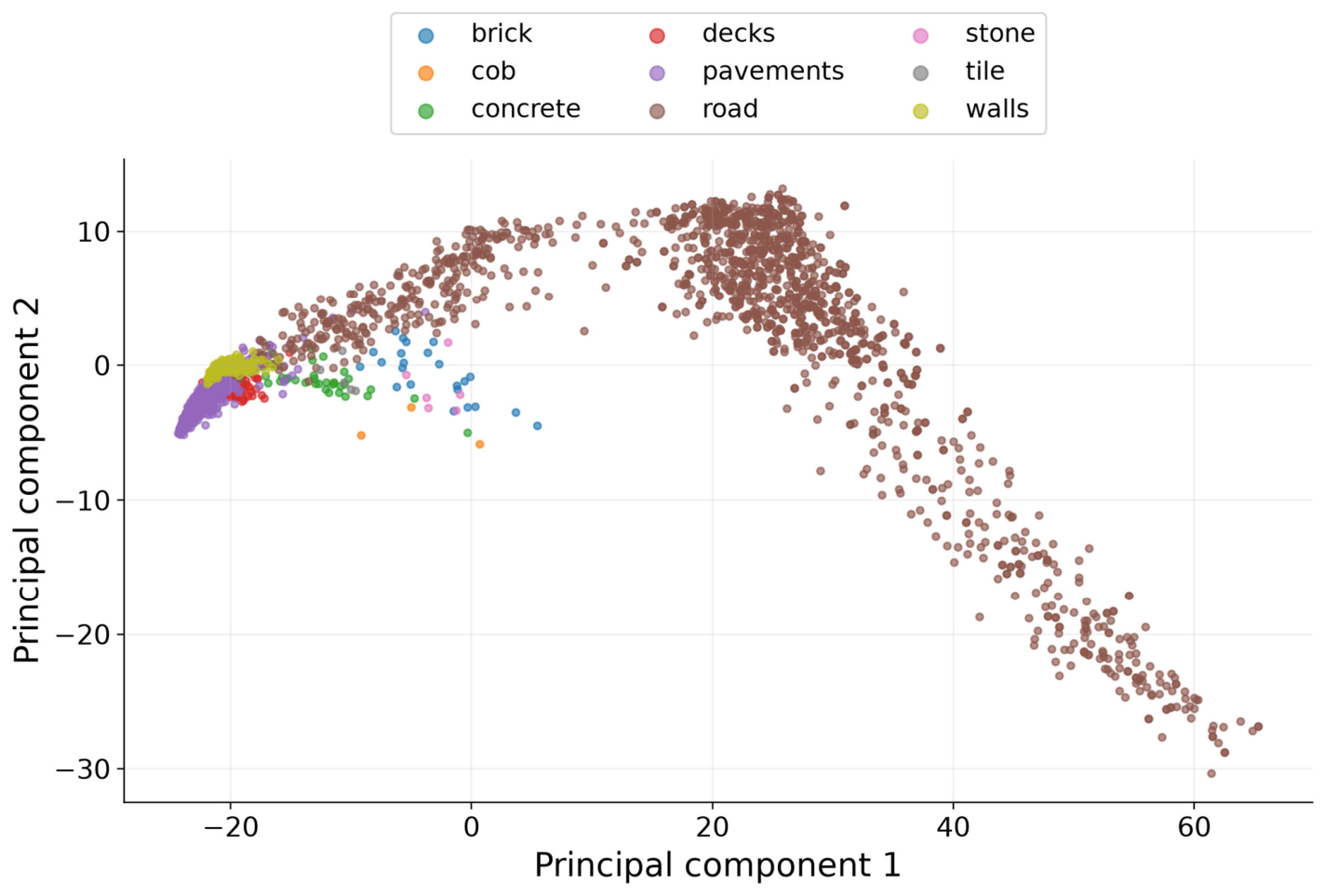
The overlays do not establish that predictions depend on crack geometry rather than material texture or acquisition context. The quantitative deletion analysis in Section 3.7 does not show an advantage over matched-area random-pixel deletion. Figure 14 exposes high-confidence surface-label errors, including walls assigned to decks. A calibrated surface classifier can still make confident mistakes and cannot be used to dismiss an apparent crack or approve an element’s structural condition. Figure 15 illustrates the PCA of 3000 test feature vectors sampled with seed 20260912.

3.5. Integrity, Source Controls, and Subset Performance

The revision verifies all 49,124 original files against the stored byte counts and SHA-256 hashes. Exact-content isolation holds, but the original grouping does not guarantee isolation of every within-class identical-dHash group. The corrected audit finds 101 cross-partition dHash groups and excludes 107 test images through union-component isolation. All 458 masonry-focused test images are retained. TokenFormer-8H changes from 99.21% to 99.19% accuracy and from 97.11% to 97.10% macro-F1. This limited sensitivity does not rule out more general visual duplication or collection-level shortcuts.

Table 9. Integrity and source diagnostics. Macro-F1 uses the supported label set stated in each row; rows with different populations are not directly interchangeable.

Experiment/Scope	Images	Accuracy %	Macro-F1 %
TokenFormer-8H: original, 9 classes	4926	99.21	97.11
TokenFormer-8H: hash-isolated, 9 classes	4819	99.19	97.10
TokenFormer-8H: masonry-focused, 5 labels	458	96.07	97.35
Source-folder majority: original, 9 classes	4926	97.97	81.85
ImageNet-only probe: original, 9 classes	4926	92.94	75.20
ImageNet-only probe: original, eligible-source subset	2700	94.37	88.31
ImageNet-only probe: held-out folders, 3 labels	26,953	83.29	61.02

separates distinct evaluation populations. The masonry-focused subset has 96.07% accuracy and 97.35% macro-F1 averaged over its five supported labels; predictions outside those labels count as errors. These subset values are not nine-class macro averages. The source-only control reaches 97.97% accuracy and 81.85% macro-F1 without using image pixels, demonstrating that acquisition-folder information is highly predictive. It does not prove that the image model directly reads metadata, but it prevents excluding source-associated visual cues as an explanation for high accuracy.

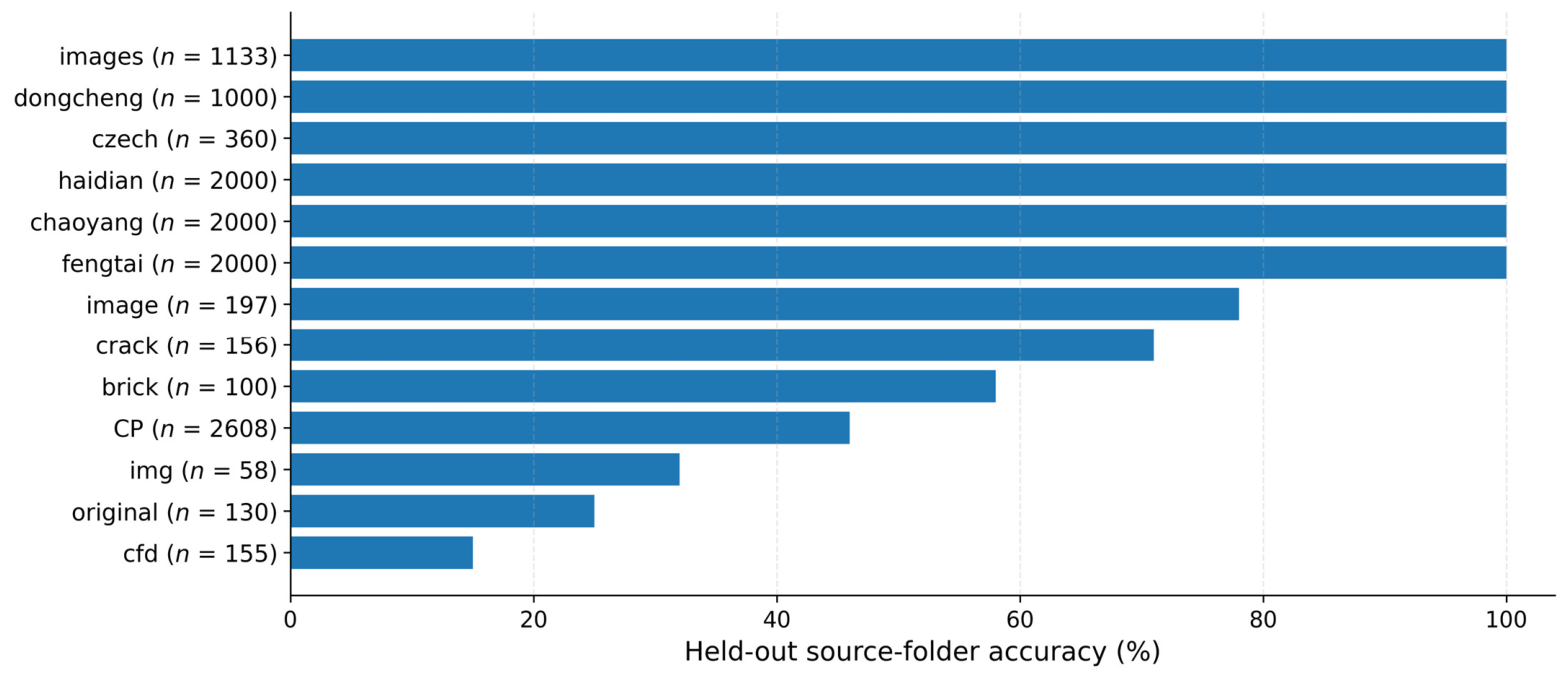
The source-held-out probe evaluates 21 folders containing 26,953 images from brick, pavements, and road; six folders cannot be evaluated because a held-out class would be absent from training. Pooled accuracy is 83.29%, three-class macro-F1 is 61.02%, and the unweighted mean of folder accuracies is 75.58%. Folder accuracy ranges from 12.90% to 100% (Figure 16). The same ImageNet-only probe reaches 94.37% accuracy on 2700 original-test images from eligible folders. These populations and fitted training pools differ, so their difference is descriptive, not a paired estimate of the selected head’s transfer loss. The fine-tuned champion itself has not been validated on an independent site.

3.6. Class-Dependent Calibration Trade-Offs

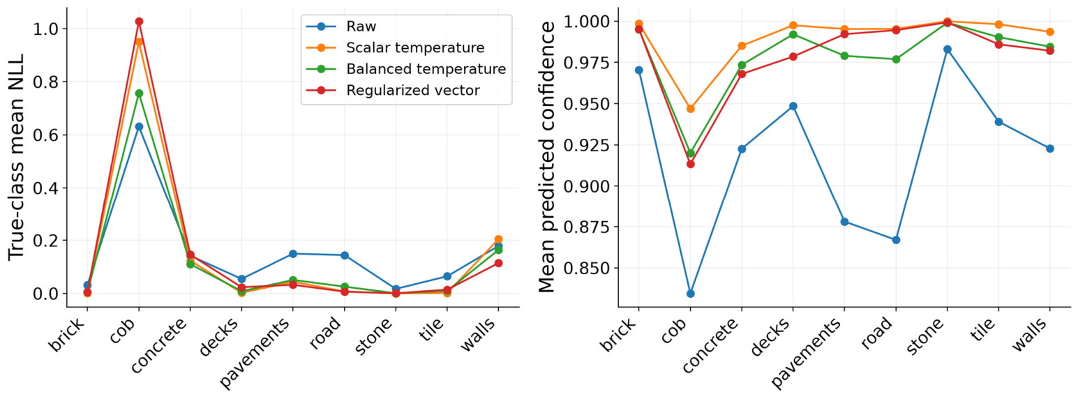
The balanced temperature is 0.652, compared with the original scalar T = 0.487. It lowers equal-class NLL from 0.1485 to 0.1259 but raises global ECE from 0.33% to 1.57%. Regularized vector scaling lowers aggregate NLL to 0.0295 and raises accuracy to 99.29%, but macro-F1 falls to 96.52% and balanced accuracy to 95.83%. Therefore, no alternative dominates every criterion. The original scalar calibration remains the reference; the higher vector-scaled test accuracy is not used to replace it. Figure 17 displays true-class mean NLL and mean predicted confidence to expose minority-class effects that a prevalence-weighted ECE can obscure.

Table 10. Validation-fitted calibration alternatives on the same 4926 test images. NLL and Brier values are unitless; no alternative is chosen using these test results.

Calibrator	Acc. %	Macro-F1 %	NLL	Equal-Class NLL	Brier	ECE %
Raw	99.21	97.11	0.1451	0.1573	0.0291	11.18
Scalar temperature	99.21	97.11	0.0398	0.1485	0.0138	0.33
Balanced temperature	99.21	97.11	0.0475	0.1259	0.0138	1.57
Regularized vector	99.29	96.52	0.0295	0.1524	0.0122	0.42

tabulates validation-fitted calibration alternatives on the same 4926 test images.

3.7. Quantitative Attribution Results

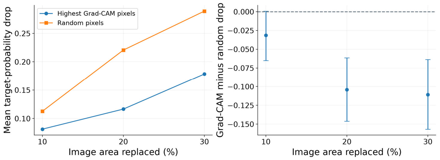
Across 323 component-distinct images, 11 Grad-CAM maps are empty. At 20% replacement, highest-attribution deletion reduces the target probability by 0.117 on average, compared with 0.221 for random-pixel deletion. The paired difference is −0.104 (95% interval −0.146 to −0.061). Results at 10% and 30% are reported in

Table 11. Grad-CAM deletion diagnostic on 323 images. Drops are calibrated target-probability differences; a positive paired difference would favor Grad-CAM-ranked deletion.

Replaced Area	Grad-CAM Drop	Random Drop	Paired Difference	95% Interval
10.00%	0.081	0.113	−0.031	−0.065 to 0.001
20.00%	0.117	0.221	−0.104	−0.146 to −0.061
30.00%	0.178	0.289	−0.111	−0.157 to −0.064

and Figure 18. These results do not demonstrate superior faithfulness of the heatmap under this test and provide no evidence of crack-specific geometry localization. Different spatial artifact patterns between the deletion masks limit causal interpretation of the comparison. No IoU or Dice score is reported because no verified crack masks are available.

3.8. Acquisition Sensitivity and Retrospective Walkthrough

The six additional full-test transformations yield accuracy from 85.71% to 99.09% and macro-F1 from 68.04% to 95.60% (

Table 12. Added synthetic acquisition-like disturbances, each evaluated on all 4926 original test images with fixed temperature.

Condition	Accuracy %	Macro-F1 %	Bal. Acc. %	ECE %
Gamma 0.7	98.84	95.27	94.15	0.49
Gamma 1.5	99.09	95.60	94.88	0.29
Spatial shadow	85.73	68.04	69.21	12.60
White balance	88.23	73.52	72.72	10.30
Perspective	85.71	73.88	75.99	10.81
JPEG quality 30	93.91	82.19	85.43	3.83

). Calibration is held fixed, so changes in ECE also indicate transfer limits of the clean-validation temperature. These additions do not replace the severe blur/noise outcomes in Section 3.4.4. A synthetic perspective warp or white-balance multiplier is not equivalent to testing an independently acquired device or environment.

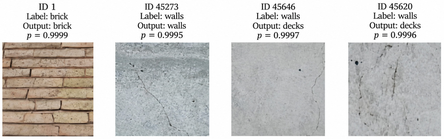
Figure 19 follows four actual stored test images through surface-label prediction. Correct brick and wall classifications coexist with highly confident wall-to-deck errors. The manifest IDs, paths, hashes, labels, and confidence values are retained in the evidence archive. The walkthrough establishes traceability of the displayed outputs only: it is retrospective, uses previously collected images, and contains no independent field inspection or structural ground truth. It therefore does not satisfy an external case-study validation claim.

4. Discussion

4.1. Positioning in Relation to Recent Works

The distinction from recent defect-localization and crack-pattern work [28,29] is the supervised target and experimental question. This study compares conditional surface-label corrections and calibration on a shared representation; it does not introduce a new detector or recover physical crack geometry. Its contribution is strengthened by explicit negative controls, a corrected integrity audit, and measured failure conditions. Source and annotation limitations prevent a claim that the benchmark advances crack-mechanism identification or is directly superior to the StructDamage source-paper architecture scores [38], whose release and evaluation setup differ.

4.2. Overall Performance Evaluation

The validation-selected head retains 99.21% accuracy and 97.11% macro-F1 on the original test partition. Residual-CNN’s 99.23% accuracy is a descriptive maximum rather than evidence for changing the selected model. The source-only control, four zero-correction heads, and component-bootstrap intervals show why a near-saturated benchmark requires interpretation beyond score ranking. The findings support accurate recognition within the observed taxonomy and collection, not a causal attribution of that accuracy to crack geometry.

Road and pavement prevalence is a property of this supplied collection, not an estimate of defect prevalence in real infrastructure. Aggregate accuracy is therefore dominated by these classes. Macro-F1, balanced accuracy, class support, the five-category masonry subset, and source-conditioned analyses expose complementary behavior, but they cannot make the collection representative of sites or material types that were not sampled.

4.3. Class-Wise Error and Minority-Category Behavior

Rare-category outcomes remain unstable because the test set contains only 10 cob, 10 stone, and 8 tile images. Perfect observed classification on a small category is not proof of generalization. The selected model’s masonry-focused accuracy is 96.07%, below its 99.21% aggregate accuracy, and its wall-to-deck errors remain practically relevant. Additional independent, expert-annotated cases are required before drawing category-specific engineering conclusions.

4.4. CNN and Attention-Family Evidence

The shared encoder isolates one narrow design choice while potentially masking differences that would emerge under end-to-end optimization. A stronger independently trained backbone might perform differently, and this experiment cannot rank full CNN or vision-transformer architectures. Four zero corrections further show that the learned representation, not the nominal head name, explains much of the reported performance. Head-only parameter counts and timings must not be interpreted as complete-model resource measurements.

4.5. Calibration and Confidence Reliability

Scalar temperature scaling improves global confidence measures on this split but does not guarantee classwise calibration. Balanced-temperature fitting reduces equal-class NLL while increasing aggregate ECE; vector scaling improves aggregate NLL but lowers macro-F1. This trade-off illustrates why a single overall reliability score is insufficient for an imbalanced taxonomy. These deterministic post-hoc calibrators are not ensembles or estimates of epistemic uncertainty. No field abstention threshold is validated, and a high category confidence cannot justify a safety decision.

4.6. Robustness and Visual Failure Analysis

The observed blur and noise failures rule out a claim of demonstrated field robustness. Macro-F1 of 46.81% under blur and 68.35% under Gaussian noise is a major limitation, not a minor degradation. The six additional acquisition-like transformations broaden sensitivity assessment but remain synthetic manipulations of low-resolution cached images. They cannot establish transfer across new cameras, weather, sites, or inspection operators. Image-quality rejection and field recalibration are requirements for future validation, not implemented guarantees.

4.7. Representation Behaviour, Explainability, and Practical Model Choice

Feature clustering and visually plausible heatmaps cannot identify the causal cue used by a classifier. The source-folder control shows that collection context is strongly predictive, and the Grad-CAM deletion experiment does not provide positive evidence of crack-specific localization. Random-pixel deletion can create more spatially dispersed artifacts than heatmap deletion, so the negative result is also conditional on the perturbation design. A fair geometric explanation study would require expert crack masks and spatially matched attribution controls; neither a mask-overlap score nor a physical mechanism is inferred here.

The practical model-selection evidence is limited to the recorded validation criterion, head size, and measured conditional performance. TokenFormer-8H remains the reproducible validation choice. GAP-MLP is a smaller candidate for future complete-pipeline evaluation, while the linear control is a necessary low-complexity reference. The small, uncertain macro-F1 differences do not justify recommending one full architecture for deployment.

Table 13. Representative high-performing recognition heads.

Method	Role in Comparison	Family	Trainable Params	Acc. %	Macro-F1 %	Bal. Acc. %	ECE %
Residual-CNN	Highest test score (descriptive)	CNN	116,554	99.23	97.16	96.90	0.42
Gated-TokenMixer	Best attention test macro-F1	Attention	101,802	99.21	97.13	96.89	0.34
Inception-CNN	Tied second test macro-F1	CNN	72,722	99.21	97.13	96.89	0.40
TokenFormer-8H	Validation-selected	Attention	101,802	99.21	97.11	96.87	0.33
GAP-MLP	Compact comparator	CNN	42,442	99.17	97.08	96.86	0.38

retains descriptive head comparisons without treating test rank as a selection rule.

The benchmark’s strongest supported conclusion is that the supplied surface categories are highly separable under the original split, while source structure, imbalance, and shared features account for much of the apparent ease. Hash-isolated reanalysis preserves high accuracy but does not remove source confounding. The deployment-relevant gaps are external site validation, crack-specific labels, acquisition robustness, and calibrated decisions under shifted conditions—not an additional fraction of a percentage point in the existing test ranking.

4.8. Engineering Scope and Required Ground Truth

Surface category is only contextual information. Distinguishing tensile, shear, shrinkage, and thermal cracking would require expert mechanism labels informed by material, loading, restraint, geometry, and history; assigning mechanisms from appearance alone would create unvalidated targets. Physical width or length requires crack delineation and a traceable scale or calibrated reconstruction with perspective correction. Width alone cannot establish residual life or hazard, which also depend on structural system, load, exposure, and deterioration history. No such quantities are inferred from resized unscaled photographs.

Likewise, compression/tension state and crack position within an element require spatial registration and structural information, not a surface-class softmax. The model has no construction-joint or non-crack output and cannot quantify a joint false-positive rate. Its confidence must not be interpreted as evidence that a visible line is a crack.

Table 14. Supported output and boundaries of engineering interpretation.

Outcome	Required Evidence	Status in This Study
Surface-category recognition	Image-level supplied category labels	Evaluated; subject to source and class imbalance
Crack mechanism/origin	Expert labels plus loading, restraint and history	Not evaluated; no verified targets
Length or opening width in mm	Crack delineation, scale and perspective calibration	Not evaluated; no physical scale
Element location and stress state	Registered coordinates, geometry and structural model	Not evaluated; no spatial or loading data
Joint versus crack rejection	Annotated joints, cracks and intact negatives	Not evaluated; no such label classes
Residual life/hazard	Structural assessment and longitudinal validation	Not supported by surface predictions
Field generalization	Independent site/device cohort and expert reference	Not established; retrospective diagnostics only

maps each requested engineering outcome to the missing ground truth. These are boundaries of the completed study.

5. Conclusions

This study evaluates all 49,124 images in the supplied original StructDamage collection using one shared encoder and twenty conditional residual-head configurations. The validation-selected TokenFormer-8H achieves 99.21% accuracy and 97.11% macro-F1; four named configurations retain zero correction. The paired macro-F1 interval over the linear control spans zero, so the benchmark does not establish a generally superior architecture. A corrected union-hash audit excludes 107 test images and retains 99.19% accuracy on 4819 images, but source-folder controls expose substantial source–category confounding. Scalar temperature scaling improves aggregate confidence measures, while class-balanced and vector alternatives reveal trade-offs hidden by ECE alone. A separate source-held-out ImageNet-only probe, quantitative attribution deletion, and eleven synthetic image-quality/acquisition conditions add diagnostic evidence without constituting external field validation. Severe blur/noise degradation and the absence of positive crack-localization evidence constrain deployment claims. The contribution is a reproducible, calibrated surface-recognition benchmark with explicit integrity and validity limits. The available data do not support crack/no-crack discrimination, mechanism classification, millimeter measurement, joint rejection, stress-state inference, residual-life prediction, or structural safety assessment. Those outcomes require new ground truth and independent site-level evaluation. High surface-category accuracy should not be substituted for those missing engineering validations.

References

1. Zou, Z.; Wang, M.; Song, B.; He, J.; Yang, S. Deep learning and digital twin driven structural health monitoring of masonry structures: Progress and challenges. Autom. Constr. 2026, 188, 106993. [Google Scholar] [CrossRef] [Scilit]
2. Zhuang, H.; Cheng, Y.; Zhou, M.; Yang, Z. Deep learning for surface crack detection in civil engineering: A comprehensive review. Measurement 2025, 248, 116908. [Google Scholar] [CrossRef] [Scilit]
3. Song, Y.; Zhang, Q.; Su, Y.; Zhang, S.; Wang, R.; Zhang, W.; Bi, Z.; Yu, Y. Advances in crack dataset development and deep learning-based detection models. J. Build. Eng. 2025, 116, 114734. [Google Scholar] [CrossRef] [Scilit]
4. Zeng, Y.; Lei, D.; He, J.; Zhou, K.; Wang, D. Deep learning-based classification of concrete crack evolution stages with reference to the double-K fracture criterion. J. Build. Eng. 2026, 119, 115176. [Google Scholar] [CrossRef] [Scilit]
5. Xu, G.; Zhang, Y.; Yue, Q.; Liu, X. A deep learning framework for real-time multi-task recognition and measurement of concrete cracks. Adv. Eng. Inform. 2025, 65, 103127. [Google Scholar] [CrossRef] [Scilit]
6. Ganduri, K.V.; Pathri, B.P.; Hemachandran, K.; Kommu, P.K.; Sharma, V.K. A deep learning and unmanned aerial vehicle framework for autonomous structural monitoring and crack detection. Eng. Appl. Artif. Intell. 2026, 182, 115922. [Google Scholar] [CrossRef] [Scilit]
7. Liu, Z.; Su, D.; Zhang, Y.; Lin, D.-W.; Sun, Z. An enhanced YOLO-based deep learning framework for automated structural defect inspection in complex backgrounds. Eng. Struct. 2026, 366, 123483. [Google Scholar] [CrossRef] [Scilit]
8. Liu, S.; Isobe, K.; Si, J.; Li, D.; Ren, D. A multi-module deep learning framework with graph-based network and crack attention for tunnel lining crack segmentation from LiDAR point cloud. Constr. Build. Mater. 2025, 494, 143383. [Google Scholar] [CrossRef] [Scilit]
9. Majidi, S.; Sharifi, M.A.; Omidalizarandi, M. Deep learning-based crack detection and 3D reconstruction for cost-effective structural health monitoring. Meas. Digit. 2026, 7, 100040. [Google Scholar] [CrossRef] [Scilit]
10. Duan, Z.; Cai, Z.; Li, Q.; Liu, Y.; Mao, Y.; Zhou, X. Adaptive deep learning framework for crack contour recognition and dimensional measurement in concrete structures. Constr. Build. Mater. 2026, 512, 145400. [Google Scholar] [CrossRef] [Scilit]
11. Jin, T.; Shou, Z.; Liu, H.; Shao, Y. Attention mechanisms and FFM feature fusion module-based modification of the deep neural network for detection of structural cracks. CMES Comput. Model. Eng. Sci. 2026, 146, 11. [Google Scholar] [CrossRef] [Scilit]
12. Dias Júnior, L.T.; Finotti, R.P.; Barbosa, F.S.; Cury, A.A. The trajectory of data-driven structural health monitoring: A review from traditional methods to deep learning and future trends for civil infrastructures. CMES Comput. Model. Eng. Sci. 2026, 146, 3. [Google Scholar] [CrossRef] [Scilit]
13. Chauhan, S.; Ranjan, R.; Dutta, B.R. A hybrid deep learning method for the crack detection and classification in surface images. Frankl. Open 2026, 16, 100705. [Google Scholar] [CrossRef] [Scilit]
14. Djerrad, A.; Zhou, Y.; Meng, S. A transformer-based deep learning framework for predicting crack patterns and structural responses in RC shear walls. Eng. Struct. 2025, 343, 121051. [Google Scholar] [CrossRef] [Scilit]
15. Ahani, E.; Yang, J. Deep learning framework for crack type detection in laminated glass based on ultrasonic and modal analysis using finite element simulations. J. Non-Cryst. Solids 2026, 676, 123950. [Google Scholar] [CrossRef] [Scilit]
16. Talaghat, M.A.; Golroo, A.; Shahhosseini, V.; Rasti, M. Fully automated pavement crack quantification and PCI estimation via a digital twin-ready vision-based deep learning pipeline. Results Eng. 2026, 32, 111659. [Google Scholar] [CrossRef] [Scilit]
17. Shah, S.M.H.; Qureshi, W.S.; O’Dea, G.; Power, D.; Ullah, I. Automated pavement condition rating for cycle routes and greenways using deep learning. Autom. Constr. 2026, 192, 107210. [Google Scholar] [CrossRef] [Scilit]
18. Zhang, Q.; Wang, C.; Xie, M.; Qi, W.; Feng, G.; Zhang, Z.; Li, Y. Soil crack healing, recurrence and the temporal persistence of preferential flow under wet-dry cycles revealed by deep-learning image analysis and breakthrough curves. Soil Tillage Res. 2026, 259, 107054. [Google Scholar] [CrossRef] [Scilit]
19. Zhang, W.; Tian, C.; Yang, J.; Xiao, P.; Wu, Z.; Li, H.; Sun, W. Vision and deep learning-based tunnel surface defect detection: Technological evolution, challenges, and prospects. Measurement 2026, 257, 118853. [Google Scholar] [CrossRef] [Scilit]
20. Li, X.; Wang, X.; Wu, S.; Guo, S.; Li, B.; Zhu, R.; Xu, L.; Li, D.; Zou, Z.; Zhang, C. Intelligent crack detection in underwater concrete structures: An image enhancement and deep learning fusion-driven approach. Case Stud. Constr. Mater. 2026, 25, e06421. [Google Scholar] [CrossRef] [Scilit]
21. Yuan, J.; Ren, Q.; Jia, C.; Zhang, J.; Fu, J.; Li, M. Automated pixel-level crack detection and quantification using deep convolutional neural networks for structural condition assessment. Structures 2024, 59, 105780. [Google Scholar] [CrossRef] [Scilit]
22. Zhuang, X.; Tran, T.V.; Nguyen-Xuan, H.; Rabczuk, T. Deep learning-based post-earthquake structural damage level recognition. Comput. Struct. 2025, 315, 107761. [Google Scholar] [CrossRef] [Scilit]
23. Liu, J.; Zhang, H.; Xiao, D. Research on defect recognition method of mine belts based on deep learning. Eng. Appl. Artif. Intell. 2026, 177, 114973. [Google Scholar] [CrossRef] [Scilit]
24. Wang, L.; Bu, B.; Zai, D.; Meng, L.; Li, J. A high-precision deep learning concrete thin crack segmentation network. Structures 2026, 92, 112936. [Google Scholar] [CrossRef] [Scilit]
25. Feng, J.; Wang, Y. Intelligent detection algorithm for concrete structure cracks based on deep learning. Procedia Comput. Sci. 2026, 281, 1095–1104. [Google Scholar] [CrossRef] [Scilit]
26. Tang, J.; Shang, Y.; Meng, J.; Li, J.; Xu, M.; Hu, Y.; Zhang, J. A new method for quantitative evaluation of micro-cracks on turbine blade surfaces fusing triboelectric sensing and hybrid deep learning. Mech. Syst. Signal Process. 2026, 247, 113947. [Google Scholar] [CrossRef] [Scilit]
27. Lu, M.; Qian, Q.; Yang, F.; Li, M. Deep learning enhanced crack identification on rocks. Artif. Intell. Geosci. 2026, 7, 100200. [Google Scholar] [CrossRef] [Scilit]
28. Ruggieri, S.; Cardellicchio, A.; Nettis, A.; Renò, V.; Uva, G. Using Attention for Improving Defect Detection in Existing RC Bridges. IEEE Access 2025, 13, 18994–19015. [Google Scholar] [CrossRef] [Scilit]
29. Cardellicchio, A.; Renò, V.; Natali, A.; Di Mucci, V.M.; Nettis, A.; Ruggieri, S.; Uva, G. An automated framework to characterize crack patterns in existing RC bridges. Data-Centric Eng. 2026, 7, e26. [Google Scholar] [CrossRef] [Scilit]
30. Aung, P.P.W.; Sam, K.M.; Kulinan, A.S.; Cha, G.; Park, M.; Park, S. Enhancing deep learning in structural damage identification with 3D-engine synthetic data. Autom. Constr. 2025, 175, 106203. [Google Scholar] [CrossRef] [Scilit]
31. Türer, A.; Bai, Y.; Sezen, H.; Yilmaz, A. Automated post-earthquake structural damage assessment of concrete buildings using a hybrid deep learning and rule-based framework on image datasets. J. Infrastruct. Intell. Resil. 2026, 5, 100208. [Google Scholar] [CrossRef] [Scilit]
32. Awan, M.R.; Chan, C.-W.; Murphy, A.; Kumar, D.; Goel, S.; McClory, C. Deep learning and image data-based surface cracks recognition of laser nitrided titanium alloy. Results Eng. 2024, 22, 102003. [Google Scholar] [CrossRef] [Scilit]
33. Aung, P.P.W.; Kulinan, A.S.; Park, M.; Ko, D.; Cha, G.; Park, S. Mitigating class imbalance in deep learning-based multi-class structural damage recognition using an informatics-oriented data augmentation framework. Adv. Eng. Inform. 2026, 71, 104430. [Google Scholar] [CrossRef] [Scilit]
34. Raza, A.; Hanif, F. COOT-CNN: A metaheuristic-optimized deep learning framework based on lightweight convolutional architectures for multi-class robust crack detection in concrete infrastructures. Ain Shams Eng. J. 2026, 17, 104293. [Google Scholar] [CrossRef] [Scilit]
35. He, X.; Liu, J.; Li, J.; Yang, Z.; Kong, X.; Zhang, Y.; Lu, Y.; Yu, Y. Toward intelligent pavement maintenance: A transferable deep learning framework for cross-domain crack segmentation and UAV-based field inspection. Adv. Eng. Inform. 2026, 73, 104582. [Google Scholar] [CrossRef] [Scilit]
36. Fan, C.; Ding, Y.; Geng, F.; Lv, Z.; Yang, K. Anomaly warning classification based on deep learning method and temperature-induced effect of bridge crack monitoring data. Eng. Struct. 2026, 352, 122158. [Google Scholar] [CrossRef] [Scilit]
37. Cui, J.; Lv, C.; Du, J. Real-time structural health monitoring of steel structures using acoustic emission signals and a KAN-LSTM deep learning framework. Eng. Struct. 2025, 344, 121328. [Google Scholar] [CrossRef] [Scilit]
38. Ijaz, M.; Khan, S.U.R.; Rehman, A.U.; Vollmer, S.; Dengel, A.; Asim, M.N. StructDamage: A Large Scale Unified Crack and Surface Defect Dataset for Robust Structural Damage Detection. arXiv 2026, arXiv:2603.10484. [Google Scholar] [CrossRef] [Scilit]
39. Zhang, Q.; Wang, S.; Cui, C.; Zhang, D. Crack detection in strengthened steel plates based on ultrasonic guided waves and deep learning. Structures 2026, 90, 112492. [Google Scholar] [CrossRef] [Scilit]
40. Li, S.; Tian, X.; Li, Q.; Ai, S. Advancing structural health monitoring: Deep learning-enhanced quantitative analysis of damage in composite laminates using surface strain field. Compos. Sci. Technol. 2024, 258, 110880. [Google Scholar] [CrossRef] [Scilit]
41. Zhao, W.; Shi, X.; Ni, F.; Tian, Y. Semi-dense sub-pixel displacement measurement for structural health monitoring: A framework of deep learning-based detector-free feature matching. Measurement 2025, 254, 117899. [Google Scholar] [CrossRef] [Scilit]
42. Bi, Q.; Sun, Y.; Yang, Y.; Sun, H. Integrated analysis of crack evolution in anchored jointed rock using Digital Image Correlation and deep learning-based detection. Appl. Comput. Geosci. 2026, 31, 100402. [Google Scholar] [CrossRef] [Scilit]
43. Wang, S.; Lin, Y.; Duan, J.; Yan, H.; Wang, X.; Xiong, X.; Huang, Y.; Guan, S.; Tao, C. Reinforcement response prediction of composite-concrete beams with crack patterns and deep learning. Comput.-Aided Civ. Infrastruct. Eng. 2025, 40, 6638–6655. [Google Scholar] [CrossRef] [Scilit]
44. Ma, Y.; Jiang, S.; Chen, X.; Sun, L.; Xue, B.; Zhang, Y. A rapid prediction method for structural fatigue life based on SBFEM and deep learning. Eng. Anal. Bound. Elem. 2026, 191, 106938. [Google Scholar] [CrossRef] [Scilit]
45. He, K.; Zhang, X.; Ren, S.; Sun, J. Deep Residual Learning for Image Recognition. In Proceedings of the IEEE Conference on Computer Vision and Pattern Recognition, Las Vegas, NV, USA, 27–30 June 2016; pp. 770–778. [Google Scholar] [CrossRef] [Scilit]
46. Guo, C.; Pleiss, G.; Sun, Y.; Weinberger, K.Q. On Calibration of Modern Neural Networks. Proc. Mach. Learn. Res. 2017, 70, 1321–1330. [Google Scholar]
47. Selvaraju, R.R.; Cogswell, M.; Das, A.; Vedantam, R.; Parikh, D.; Batra, D. Grad-CAM: Visual Explanations from Deep Networks via Gradient-Based Localization. In Proceedings of the IEEE International Conference on Computer Vision, Venice, Italy, 22–29 October 2017; pp. 618–626. [Google Scholar] [CrossRef] [Scilit]
Figure 1. Structural surface image formation and crack-confounder mechanisms.
Applsci 16 09337 g001
Figure 2. Actual test photographs representing the nine supplied surface categories. Category labels are not crack-mechanism or geometric annotations.
Applsci 16 09337 g002
Figure 3. Natural class distribution of the complete structural-image corpus.
Applsci 16 09337 g003
Figure 4. Integrity-controlled image audit, grouping, and partition pathway. The displayed zero overlap refers to the stored original group identifiers, not all perceptual matches. The corrected union-hash audit identifies 101 cross-partition within-class equal-dHash groups (Table 2).
Applsci 16 09337 g004
Figure 5. Class composition of each original partition. Percentages are normalized within each partition; sample counts are shown below the bars.
Applsci 16 09337 g005
Figure 6. Matched residual-head recognition and validation-only calibration framework. The purple path denotes sequential validation operations: macro-F1 selects the head, whereas NLL separately fits the temperature. Residual logit fusion combines the base logits with one gated correction, as specified in Equation (7).
Applsci 16 09337 g006
Figure 7. Common ResNet-18 encoder with alternative convolutional and attention-based recognition branches and calibrated output. The branches depict separate head experiments, not a joint ensemble. Residual logit fusion combines the base logits (omitted from this overview) with one sigmoid-gated correction, as specified in Equation (7).
Applsci 16 09337 g007
Figure 8. Paired macro-F1 differences from the linear control with 95% union-component bootstrap intervals (5000 resamples). Squares mark zero-correction configurations. Intervals are unadjusted descriptive intervals, not simultaneous family-wise confidence bounds.
Applsci 16 09337 g008
Figure 9. Accuracy versus macro-F1 for conditional head configurations. Numeric keys avoid overlapping model names; the square combines the linear control and four identical zero-correction outputs. The displayed axes are restricted to the observed score range.
Applsci 16 09337 g009
Figure 10. All head-level observations by family. Squares indicate selected zero-correction heads and horizontal lines indicate descriptive means. The shared encoder precludes an independent-backbone interpretation.
Applsci 16 09337 g010
Figure 11. Row-normalized confusion matrix for the validation-selected TokenFormer-8H.
Applsci 16 09337 g011
Figure 12. Reliability before and after scalar temperature scaling on the same test set. Points are non-empty equal-width confidence bins; low-confidence bins contain few images and should not be interpreted as precise reliability estimates.
Applsci 16 09337 g012
Figure 13. Original photographs beside layer-3 Grad-CAM overlays for six cases from the component-distinct attribution sample. Manifest IDs provide traceability; images are selected without conditioning on correct prediction. Overlays are score attributions, not crack masks or geometric ground truth.
Applsci 16 09337 g013
Figure 14. Six actual test misclassifications with the highest calibrated confidence, selected deterministically without image synthesis. Titles report supplied label, predicted surface category, confidence, and manifest ID.
Applsci 16 09337 g014
Figure 15. PCA of 3000 test feature vectors sampled with seed 20260912. The projection is descriptive and does not separate material, acquisition-source, and crack-morphology causes of clustering.
Applsci 16 09337 g015
Figure 16. Leave-source-folder-out accuracy of the separate ImageNet-only ridge probe. Training excludes the held-out folder and matching hash components. All 21 eligible folders are shown. Source-folder names are reproduced exactly from the dataset directory structure; similarly named folders (e.g., dongcheng_JPEGImages and dongcheng_images2, and fengtai_JPEGImages and fengtai_images2) are distinct source folders and were treated independently.
Applsci 16 09337 g016
Figure 17. Class-conditional NLL and mean predicted confidence for four calibration conditions. Each class contributes equally to equal-class NLL; rare-class estimates remain based on 8–10 images.
Applsci 16 09337 g017
Figure 18. Attribution-directed versus random-pixel deletion and paired 95% bootstrap intervals. Neither plot is a crack-localization accuracy measure.
Applsci 16 09337 g018
Figure 19. Traceable retrospective image walkthrough: two correct surface classifications and two highest-confidence errors. These are existing test photographs, not a new field case study or physical crack measurement.
Applsci 16 09337 g019