An Adaptive OVMD-SSA-GRU Hybrid Framework for Highway Soft Rock Slope Deformation Prediction

Featured Application

The proposed OVMD-SSA-GRU framework can be integrated into automated highway slope monitoring and early-warning platforms to provide deformation forecasts for rainfall-sensitive soft rock slopes.

Abstract

Highway soft rock slope deformation monitoring produces nonlinear, non-stationary, and multi-scale time series that are strongly affected by rainfall and field noise. This study proposes an adaptive hybrid framework that combines optimal variational mode decomposition (OVMD), the sparrow search algorithm (SSA), and gated recurrent unit (GRU) networks. High-precision BeiDou Global Navigation Satellite System (GNSS) observations collected hourly over a 120-day K55 monitoring campaign (late 2022 to early 2023) are cleaned using a cumulative-sum (CUSUM) change-point detector and cubic-spline reconstruction, while rainfall-related hydro-mechanical variables derived from seepage and slope-stability analyses are incorporated as external inputs. To prevent future-information leakage during blind testing, OVMD is recomputed causally at each one-day-ahead forecast origin using only observations available up to that origin; it then separates the deformation signal into physically interpreted trend, periodic, and high-frequency components, and SSA adaptively optimizes component-specific GRU hyperparameters for parallel prediction and reconstruction. On the K55 strongly weathered shale slope, across five independent runs the proposed model achieved a mean root-mean-square error (RMSE) of 0.04 ± 0.01 mm and a mean absolute percentage error (MAPE) of 0.18 ± 0.05%, outperforming standard GRU, long short-term memory (LSTM), and back-propagation neural network (BPNN) baselines that received an equivalent validation-based hyperparameter search. Cross-scenario evaluation on a geologically distinct K14 marl slope, independently retrained on its own record, yielded a mean RMSE of 0.14 ± 0.02 mm and a mean MAPE of 0.42 ± 0.08%. The results indicate that the proposed framework improves prediction accuracy while retaining useful cross-scenario robustness, supporting intelligent monitoring and early warning of rainfall-sensitive highway slopes.

1. Introduction

With the rapid development of transportation infrastructure, the stability of highway slopes in complex geological environments has become an increasingly important safety concern. Soft-rock cut slopes are particularly susceptible to progressive deformation under the coupled effects of geological structures, rainfall infiltration, excavation disturbance, freeze-thaw action, and long-term environmental loading. These processes may lead to creep, progressive sliding, and ultimately instability, threatening highway operation and surrounding infrastructure [1,2].

Accurate slope-deformation prediction is therefore a key component of intelligent monitoring and early-warning systems. Conventional approaches include deterministic numerical methods, grey-system models, empirical/statistical models, and nonlinear time-series methods. Although these approaches have achieved useful results, deterministic models depend strongly on difficult-to-obtain geotechnical parameters, while statistical models can be sensitive to noise and may struggle with strongly nonlinear and non-stationary deformation sequences [3,4,5,6,7,8,9,10,11,12,13,14,15,16].

In recent years, machine-learning and deep-learning methods have provided new approaches for slope-deformation prediction. Gated recurrent architectures such as the long short-term memory (LSTM) network and the gated recurrent unit (GRU) are particularly attractive because they can capture long-range temporal dependence in monitoring sequences; the GRU simplifies the gating structure of the LSTM while retaining memory capability and typically requiring fewer trainable parameters [17,18]. Nevertheless, model performance remains sensitive to input quality, noise contamination, and hyperparameter selection.

Beyond individual predictors, a growing body of work combines statistical or physical components with data-driven learners for time-dependent geotechnical forecasting. Jamhiri et al. [19] hybridized a neural network with trend-adjusted exponential smoothing to forecast the time-dependent resistance of stabilized fine sands under rapid shearing; Bagheri et al. [20] coupled a time-series module with physics-informed machine learning to predict soil water content; and Hong et al. [21] developed LSTM-Transformer hybrids for consolidation-settlement prediction. These studies show that decomposition-learning and physics-informed hybridization can outperform single networks, but most are validated on laboratory specimens or a single field site, and none jointly addresses adaptive mode-number selection, swarm-based component-wise tuning, and cross-geology re-application on highway soft-rock slopes. The present study positions itself within this hybrid-modelling class while explicitly filling these gaps.

Direct prediction from raw GNSS deformation series remains challenging because the monitored signals are nonlinear, non-stationary, multi-scale, and contaminated by high-frequency disturbances arising from multipath effects, atmospheric delays, construction vibration, and sensor noise. These characteristics can obscure the long-term deformation trend and lead to overfitting or prediction lag.

Signal-decomposition methods provide an effective way to separate these mixed temporal scales before forecasting. Variational mode decomposition (VMD) decomposes a complex signal into band-limited intrinsic mode functions (IMFs) and has been widely applied to non-stationary engineering signals because of its frequency localization and noise robustness [22,23,24,25]. However, its performance depends on decomposition parameters, particularly the mode number K and the penalty factor α.

Population-based optimization can further reduce dependence on manual network tuning. The sparrow search algorithm (SSA) is a swarm-intelligence optimizer inspired by sparrow foraging and anti-predation behavior and has shown strong global-search capability in nonlinear optimization problems [26,27]. In this study, SSA is used to adaptively optimize key GRU parameters.

Accordingly, this study proposes an adaptive OVMD-SSA-GRU (OSG) hybrid framework for highway soft rock slope deformation prediction. The specific objectives are: (i) to build a physically informed, noise-robust input pipeline from raw GNSS and rainfall records; (ii) to decompose the non-stationary deformation series into trend, periodic, and random components using an adaptively determined VMD; (iii) to tune component-specific GRU predictors with SSA rather than trial-and-error; and (iv) to validate the resulting one-day-ahead forecaster on two geologically distinct slopes. Relative to using GRU, LSTM, or BPNN alone, the framework is expected to improve accuracy by removing mixed-scale interference before learning and by matching network capacity to each component dynamics. The main contributions are as follows:

(1)

A systematic feature-engineering workflow integrating CUSUM change-point detection, cubic-spline reconstruction, and numerically informed hydro-mechanical driving factors is established to improve the quality and physical interpretability of the monitoring inputs.

(2)

An adaptive OVMD strategy based on the evolution of adjacent modal center frequencies is introduced to separate the deformation signal into physically interpretable trend, periodic, and random components while reducing modal mixing.

(3)

SSA is used to perform global adaptive optimization of GRU hyperparameters, reducing reliance on trial-and-error tuning and enabling component-specific parallel prediction.

(4)

The framework is evaluated on two geologically heterogeneous highway slope scenarios (strongly weathered shale and marl), providing a cross-scenario assessment of prediction robustness and engineering applicability.

The remainder of this paper is organized as follows. Section 2 introduces the methodology, including OVMD decomposition, SSA optimization, and GRU prediction. Section 3 presents the engineering case and data processing procedures. Section 4 discusses the prediction results and comparative analysis. Section 5 provides further discussion, and Section 6 concludes the study.

2. Materials and Methods

2.1. Data Preprocessing

Slope deformation monitoring data usually contain nonlinear fluctuations, random disturbances, and measurement noise caused by complex geological conditions and environmental factors. Directly applying raw monitoring sequences to prediction models may reduce learning efficiency and affect prediction stability. Therefore, appropriate preprocessing is required before model training.

In this study, the collected slope deformation monitoring sequence was first normalized to eliminate the influence of different scales among data points. The normalization process can be expressed as:

$${x_i}^{\ast }={\displaystyle \frac{x_i-x_{\mathrm{m}\mathrm{i}\mathrm{n}}}{x_{\mathrm{m}\mathrm{a}\mathrm{x}}-x_{\mathrm{m}\mathrm{i}\mathrm{n}}}}.$$

(1)

where $x_i$ is the original monitoring value, $x_{\mathrm{m}\mathrm{i}\mathrm{n}}$ and $x_{\mathrm{m}\mathrm{a}\mathrm{x}}$ are the minimum and maximum values of the sequence, respectively, and ${x_i}^{\ast }$ is the normalized value.

The GNSS displacement series was originally recorded at 1 h intervals by the BeiDou stations. The continuous K55 monitoring campaign covered 120 days from late 2022 to early 2023, spanning the wet-to-dry seasonal transition that contains the rainfall-induced deformation events of interest. To maintain temporal consistency with the daily rainfall-related input variables and with the one-day-ahead forecasting horizon, the hourly records were aggregated to a daily scale. Rather than averaging the twenty-four hourly readings, which would smear abrupt rainfall-induced jumps and inflate the residual, the last valid cumulative-displacement observation of each day (around 23:00 local time) was retained as the representative daily value; this choice preserves the end-of-day cumulative displacement that best reflects the net effect of that day’s rainfall and creep accumulation. After temporal alignment and quality control, a continuous 120-day deformation sequence was used for modeling. The samples were divided strictly in chronological order without random shuffling: days 1–72 for training, days 73–90 for validation and hyperparameter optimization, and days 91–120 as an independent blind-testing period (60%, 15%, and 25% of the complete sequence, respectively).

To avoid information leakage, all preprocessing and parameter-selection procedures followed a strict causal (rolling-origin) temporal-validation strategy. Normalization parameters were estimated on the training data only and then fixed for validation and blind testing. The CUSUM anomaly criteria and spline settings were determined without using blind-test observations. Critically, OVMD was not applied once to the full 120-day series. At each one-day-ahead forecast origin t, the decomposition was recomputed from scratch using only the deformation observations available up to t; the adaptive center-frequency stopping rule, the retained mode count, and the component-wise SSA-GRU weights were likewise re-estimated on the expanding training window and frozen when producing the next-day forecast. Equivalently, no post-origin samples entered the variational optimization that produced the IMF components at time t, so future rainfall or creep information could not propagate into the blind-test components. Normalization, decomposition, and component forecasts therefore respect the information set {y_1, …, y_{t-1}} at every t, and the reported blind-test metrics represent genuine out-of-sample one-day-ahead performance.

Considering that slope deformation is affected by multiple external factors and exhibits complex temporal dependencies, the processed sequence was further decomposed into several components using the proposed OVMD method before prediction.

2.2. Optimal Variational Mode Decomposition (OVMD)

Variational mode decomposition (VMD), originally proposed by Dragomiretskiy and Zosso [22], is an adaptive time-frequency analysis method that decomposes a complex signal into several band-limited intrinsic mode functions (IMFs). Subsequent studies have demonstrated its usefulness for non-stationary engineering signals and adaptive signal decomposition [23,24,25].

The standard VMD variational formulation follows Dragomiretskiy and Zosso [22]. For the adaptive center-frequency criterion used in this study, the center frequency of the kth mode is calculated as:

$${\omega }_k={\displaystyle \frac{{\displaystyle {\int }_0^{\infty }}\omega {\left|U_k\left(\omega \right)\right|}^2\mathrm{d}\mathsf{\omega }}{{\displaystyle {\int }_0^{\infty }}{\left|U_k\left(\omega \right)\right|}^2\mathrm{d}\mathsf{\omega }}}.$$

(2)

where u_k(t) is the kth intrinsic mode function, K is the number of decomposed modes, ω_k is the center (angular) frequency of the kth mode, U_k(ω) is the Fourier transform of u_k(t), and ω denotes angular frequency; the center frequency is the spectral centroid of the kth mode, i.e., the frequency at which its spectral energy is concentrated.

Although VMD provides an adaptive decomposition strategy, its performance is significantly influenced by key parameters, especially the number of modes K and the penalty factor α. Improper parameter selection may result in over-decomposition or insufficient feature extraction.

To reduce the dependence of conventional VMD on manually selected decomposition settings, an adaptive center-frequency criterion was adopted. During iterative decomposition, adjacent modal center frequencies were monitored; overlap or a center-frequency ratio approaching unity (i.e., a ratio above 0.95) was treated as evidence of over-decomposition and triggered acceptance of the current mode number. The penalty factor and update/noise-tolerance parameter were set to α = 2000 and τ = 0, respectively. For the K55 case this criterion converged to three retained component groups (IMF1-IMF3), interpreted as trend, periodic, and high-frequency random behavior. As stated in Section 2.1, this adaptive search was performed recursively on the causal data window at each forecast origin rather than once on the full future-augmented series. The resulting three-component representation is used consistently in all subsequent prediction and reconstruction results.

A residual evaluation index of reconstruction error intensity (IREI), constructed from the root-mean-square reconstruction residual, is used to assess decomposition fidelity:

$$I_{\mathrm{R}\mathrm{E}\mathrm{I}}=\sqrt{{\displaystyle \frac{1}{M}}{\displaystyle {\sum }_{i=1}^M}{\left[{\displaystyle {\sum }_{k=1}^K}{u}_k\left(t_i\right)-f\left(t_i\right)\right]}^2}.$$

(3)

where I_REI is the reconstruction-error intensity index, M is the number of samples, K is the number of decomposed modes, u_k(t_i) is the kth intrinsic mode at the ith sample, and f(t_i) is the original measured displacement at the ith sample. A smaller I_REI indicates a more faithful decomposition.

Compared with directly using the original deformation sequence, OVMD can separate:

(1)

long-term deformation trends;

(2)

periodic environmental responses;

(3)

high-frequency random disturbances.

Therefore, OVMD improves the representation capability of slope deformation signals and provides more reliable inputs for prediction models. The temporal-frequency characteristics and physical interpretation of the retained components are analyzed quantitatively in Section 4.1.

2.3. Sparrow Search Algorithm (SSA)

The sparrow search algorithm (SSA), proposed by Xue and Shen [26], is a population-based optimization method inspired by sparrow foraging and anti-predation behavior. Individuals are divided into discoverers, followers, and scouts/warners, whose coordinated position updates balance global exploration and local exploitation. Recent reviews summarize SSA among widely used swarm-intelligence optimization approaches [27].

Discoverers are responsible for searching promising regions of the solution space, while followers update their positions according to the information provided by discoverers. Warners adjust their positions when potential danger is detected, improving the global exploration capability of the algorithm.

The discoverer, follower, and warning-agent positions were updated according to the standard SSA rules of Xue and Shen [26]. In the present implementation, the optimization objective was the prediction RMSE:

$$\mathrm{F}\mathrm{i}\mathrm{t}\mathrm{n}\mathrm{e}\mathrm{s}\mathrm{s}=\sqrt{{\displaystyle \frac{1}{M}}{\displaystyle {\sum }_{m=1}^M}{\left(y_m-{\widehat{y}}_m\right)}^2}.$$

(4)

where $M$ is the number of validation samples, $y_m$ is the measured value, and ${\widehat{y}}_m$ is the predicted value.

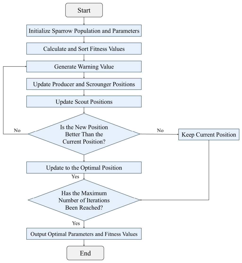
Through iterative optimization, SSA searches for the parameter combination that minimizes the prediction error. The root-mean-square error (RMSE) evaluated on the model-development data is used as the fitness criterion.

In this study, the GRU hidden-unit configuration (number of hidden units and dropout) and the learning rate are mapped to the position vector of each sparrow. The SSA population size is 30 and the maximum number of iterations is 50. Discoverers account for 20% of the population, followers for 80%, and 15% of individuals participate in the warning/scouting mechanism. Validation RMSE on the training/validation split is used as the fitness criterion. To ensure a fair comparison, the standard GRU, LSTM, and BPNN baselines received the same validation-based hyperparameter search (a grid search over hidden size and learning rate with the same early-stopping rule), and every architecture was independently rerun five times with different random seeds; the metrics reported below are mean ± standard deviation over the five runs.

Separate SSA searches were conducted for IMF1, IMF2, and IMF3 so that the GRU hidden-unit configuration and learning rate could adapt to the distinct dynamics of each decomposed component.

The SSA optimization procedure is summarized in Figure 1.

2.4. Gated Recurrent Unit (GRU)

GRU is an improved recurrent neural network structure designed to overcome the vanishing-gradient problem of traditional recurrent neural networks. Compared with LSTM, GRU has a simpler structure and fewer parameters while maintaining strong temporal feature extraction capability.

The GRU structure mainly consists of update gates and reset gates. The update gate controls the proportion of previous information retained, while the reset gate determines the influence of previous hidden states on current information.

The update gate can be expressed as:

$$z_t=\sigma \left(W_z\left[h_{t-1},x_t\right]+b_z\right).$$

(5)

The reset gate is defined as:

$$r_t=\sigma \left(W_r\left[h_{t-1},x_t\right]+b_r\right).$$

(6)

The hidden state is updated through:

$${\tilde{h}}_t=\mathrm{t}\mathrm{a}\mathrm{n}\mathrm{h}\left(W_h\left[r_t\odot h_{t-1},x_t\right]+b_h\right).$$

(7)

$$h_t=\left(1-z_t\right)\odot h_{t-1}+z_t\odot {\tilde{h}}_t.$$

(8)

where $z_t$ and $r_t$ are the update and reset gates, respectively; $x_t$ is the input vector; $h_{t-1}$ and $h_t$ are the previous and current hidden states; ${\tilde{h}}_t$ is the candidate hidden state; $W$ and $b$ denote trainable weights and biases; $\sigma$ is the logistic sigmoid function; and $\odot$ denotes element-wise multiplication.

Due to its ability to capture long-term temporal dependencies, GRU is suitable for slope deformation prediction problems involving continuous monitoring sequences.

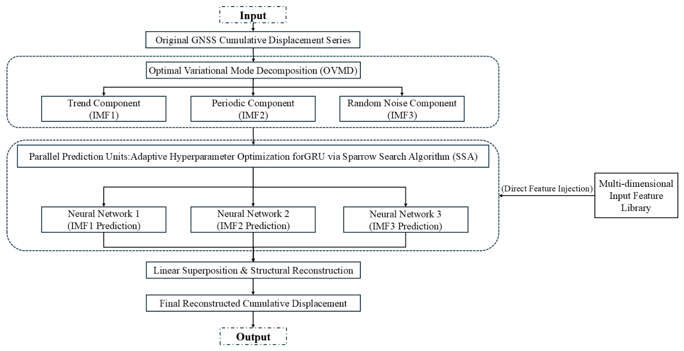
The prediction task was formulated as sequential one-day-ahead forecasting on the daily aligned series described in Section 2.1. The same GRU formulation was used for all three parallel branches, while the hidden-unit configuration and learning rate of each branch were adaptively selected by the component-specific SSA search. Each optimized branch produced the next-day estimate of its corresponding IMF, and the three component forecasts were then reconstructed to obtain total cumulative displacement.

2.5. Proposed OVMD-SSA-GRU Prediction Framework

Based on the above methods, an integrated OVMD-SSA-GRU framework is proposed for highway soft rock slope deformation prediction.

The complete prediction procedure includes the following steps:

(1)

The original slope deformation monitoring sequence is normalized to reduce scale differences.

(2)

OVMD is applied to decompose the original sequence into several IMF components with different temporal-frequency characteristics.

(3)

SSA is employed to optimize the key parameters of GRU networks.

(4)

Each decomposed component is independently predicted using the optimized GRU model.

(5)

The prediction results of all components are reconstructed to obtain the final deformation prediction value.

The overall workflow of the proposed framework is shown in Figure 2.

Compared with traditional single-model prediction approaches, the proposed framework combines signal decomposition, parameter optimization, and deep learning prediction, which improves the capability of capturing complex nonlinear deformation characteristics.

2.6. Evaluation Metrics

Prediction performance was evaluated using mean absolute error (MAE), root-mean-square error (RMSE), mean absolute percentage error (MAPE), and the coefficient of determination (R²):

$$\mathrm{M}\mathrm{A}\mathrm{E}={\displaystyle \frac{1}{N}}{\displaystyle {\sum }_{i=1}^N}\left|y_i-{\widehat{y}}_i\right|,$$

(9)

$$\mathrm{R}\mathrm{M}\mathrm{S}\mathrm{E}=\sqrt{{\displaystyle \frac{1}{N}}{\displaystyle {\sum }_{i=1}^N}{\left(y_i-{\widehat{y}}_i\right)}^2},$$

(10)

$$\mathrm{M}\mathrm{A}\mathrm{P}\mathrm{E}={\displaystyle \frac{100}{N}}{\displaystyle {\sum }_{i=1}^N}\left|{\displaystyle \frac{y_i-{\widehat{y}}_i}{y_i}}\right|,$$

(11)

$$R^2=1-{\displaystyle \frac{{\displaystyle {\sum }_{i=1}^N}{\left(y_i-{\widehat{y}}_i\right)}^2}{{\displaystyle {\sum }_{i=1}^N}{\left(y_i-\overline{y}\right)}^2}}.$$

(12)

where $y_i$ and ${\widehat{y}}_i$ denote measured and predicted displacement, respectively; $\overline{y}$ is the mean measured displacement; and $N$ is the number of evaluation samples. Error metrics in millimeters were calculated on the physical displacement scale after inverse transformation.

All MAE and RMSE values reported in the Results section are expressed in millimeters on the physical displacement scale, and MAPE is evaluated over the same chronologically held-out blind-test samples used for the corresponding model comparisons.

3. Case Study and Data Preprocessing

3.1. Engineering Geological Background and Intelligent Monitoring Layout

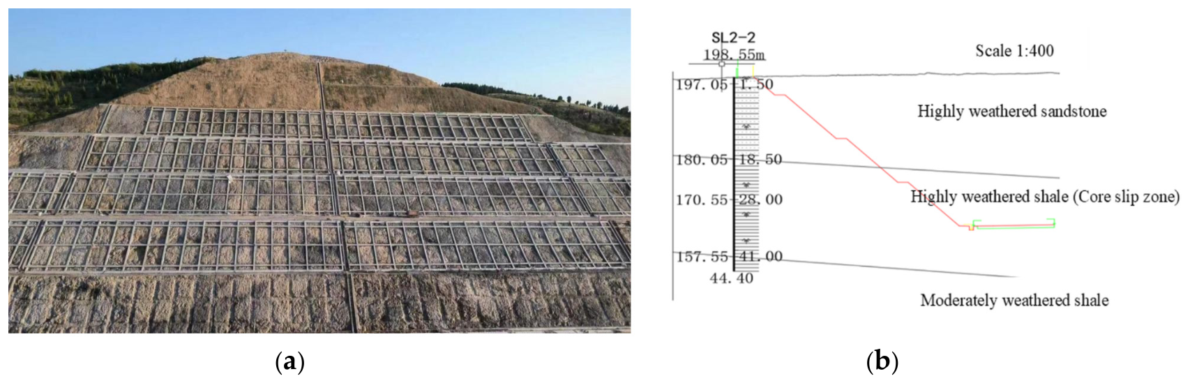
The field experimental site is located at a typical high-slope bedding cutting segment in soft rock (Chainage: K55+150–K55+600) along a target highway. The slope has a total length of 450 m, a maximum vertical excavation height of 32 m, and adopts a three-tier platform stepped protection structure. The engineering area belongs to a typical low-mountain and hilly landform with complex geological structures. According to the representative K55+400 geological cross-section, the stratigraphy comprises Quaternary loose gravel and clay fill (0.5–1.1 m thick), Permian strongly weathered sandstone (0.8–9.1 m thick), a strongly weathered shale zone containing the principal slip surface and core weakness zone (2.9–13.6 m thick), and an underlying moderately weathered shale unit. The strongly weathered shale exhibits pronounced water sensitivity and slaking, with a marked reduction in shear strength after rainfall infiltration and strong creep deformation. The engineering setting and representative cross-section are shown in Figure 3.

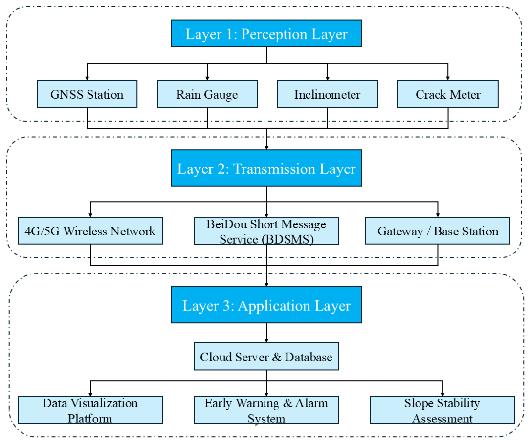
Automated, high-precision full-constellation BeiDou GNSS displacement stations, tipping-bucket rain gauges, fixed inclinometers, and wireless pull-wire crack meters were deployed at the site [28]. The K55+400 geological cross-section is located in the main potential sliding zone, where the GNSS station on the third-tier platform provides high-density horizontal and vertical deformation time series at a 1 h sampling interval. The intelligent monitoring architecture is shown in Figure 4.

3.2. Anomalous Data Cleaning and Cubic Spline Smoothing

Field monitoring data inevitably suffer from random measurement errors and coarse outliers induced by harsh outdoor environments. For instance, on 11 November 2022 at 06:00, the horizontal cumulative deformation value abruptly jumped to 0 mm, while adjacent measurements at 05:00 and 07:00 recorded 37.81 mm and 37.92 mm, respectively. This step-wise anomaly violates the physical continuity of soft rock creep behavior.

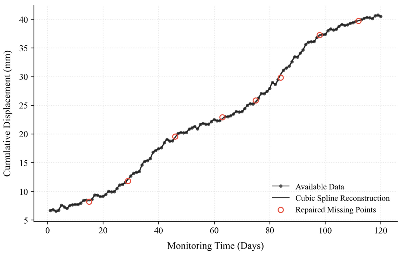
To clean the raw series, a Cumulative Sum (CUSUM) change-point detector was applied to the hourly displacement-increment series. A two-sided CUSUM with a sliding baseline window of 7 days (168 hourly samples) monitored the cumulative mean deviation; the reference shift k was set to 0.5σ of the local hourly-increment standard deviation, and the decision threshold h was set to 5σ (corresponding to an in-control false-alarm rate of about one per 1000 observations under the Gaussian assumption). Points whose cumulative statistic breached h were flagged as candidate anomalies; they were then additionally checked against adjacent GNSS observations and the smooth creep expected for soft rock, and an isolated jump exceeding 3σ of the local hourly-increment standard deviation between two otherwise consistent readings was rejected. In total, 23 hourly readings out of the 2880 hourly K55 observations (about 0.8%) were removed as gross sensor failures; no genuine rainfall-induced step change was discarded because its magnitude was physically consistent with the surrounding seepage response. Subsequently, cubic spline interpolation with continuous first- and second-order derivatives at internal knots was applied to the resulting gaps before the cleaned hourly series was aggregated to the daily scale, restoring an equal-interval, high-fidelity training sequence (Figure 5).

The CUSUM procedure therefore identifies only isolated gross anomalies characterized by abrupt cumulative deviations from the local deformation evolution; because the detector and the rejection rule were fixed on the training window and the spline interpolation preserves the overall trajectory, genuine short-duration rainfall responses are not suppressed by subjective smoothing.

3.3. Hydro-Mechanical Input Feature Library via Seepage Numerical Simulation

To establish physically meaningful external input variables, mechanism-informed seepage/stability analyses were conducted for the K55+400 section using the SEEP/W and SLOPE/W modules of GeoStudio (GEO-SLOPE International Ltd., Calgary, AB, Canada) under different rainfall scenarios. The numerical analysis was used to support selection of hydro-mechanical driving factors for the data-driven forecasting model.

The SEEP/W model discretized the K55+400 cross-section into ≈2400 quadrilateral elements. The strongly weathered shale was assigned a saturated volumetric water content of 0.38, a saturated hydraulic conductivity of 1.2 × 10⁻⁶ m/s, and a van Genuchten retention curve with α = 0.05 kPa⁻¹ and n = 1.6; the overlying fill and the moderately weathered bedrock used values from site laboratory tests. The slope surface was assigned a rainfall-flux boundary equal to the reported hyetograph (ponding limited by saturated conductivity), the bedrock base a free-drainage boundary, and the lateral sides a no-flow boundary. The effective shear strength used in SLOPE/W was c′ = 18 kPa and φ′ = 24°, calibrated so that the simulated natural-state factor of safety (FoS) of 1.297 reproduced the observed stable, sub-millimetre-per-day creep; under the 80 mm/d 24-h rainfall scenario the computed FoS decreased to 1.183, consistent with the accelerated creep phase recorded by the GNSS station during the same event. The 3-day antecedent window was selected objectively by comparing Spearman rank correlations between cumulative displacement and antecedent rainfall accumulated over 1, 3, 5, 7, and 10 days: the 3-day window gave the strongest rank correlation (ρ = 0.78, p < 0.01) and was retained rather than chosen a priori.

(1)

Under a heavy-rainfall scenario with daily rainfall > 80 mm/d, rapid infiltration along unloading fractures increases pore-water pressure and reduces matrix suction in the strongly weathered shale, producing the factor-of-safety reduction and the nonlinear acceleration of deformation quantified by the calibrated numerical model above.

(2)

Spearman rank-correlation screening indicated positive associations between cumulative displacement and both current daily rainfall and antecedent cumulative rainfall. These rainfall variables were therefore retained as external driving features together with deformation-history terms; no inferential significance claim is made beyond the reported variable-selection role.

Based on these geomechanical response mechanisms, a multi-dimensional hydro-mechanical input feature library was defined: antecedent cumulative displacement, antecedent deformation rate, current daily rainfall, 3-day antecedent cumulative rainfall, and 3-day cumulative deformation increment.

Accordingly, the seepage/stability analysis serves as a mechanism-informed feature-selection step rather than as a stand-alone calibrated prediction model; deformation forecasting is performed by the OVMD-SSA-GRU framework using the monitoring-derived feature library described above.

4. Results and Analysis

4.1. Analysis of Time-Frequency Decomposition Characteristics

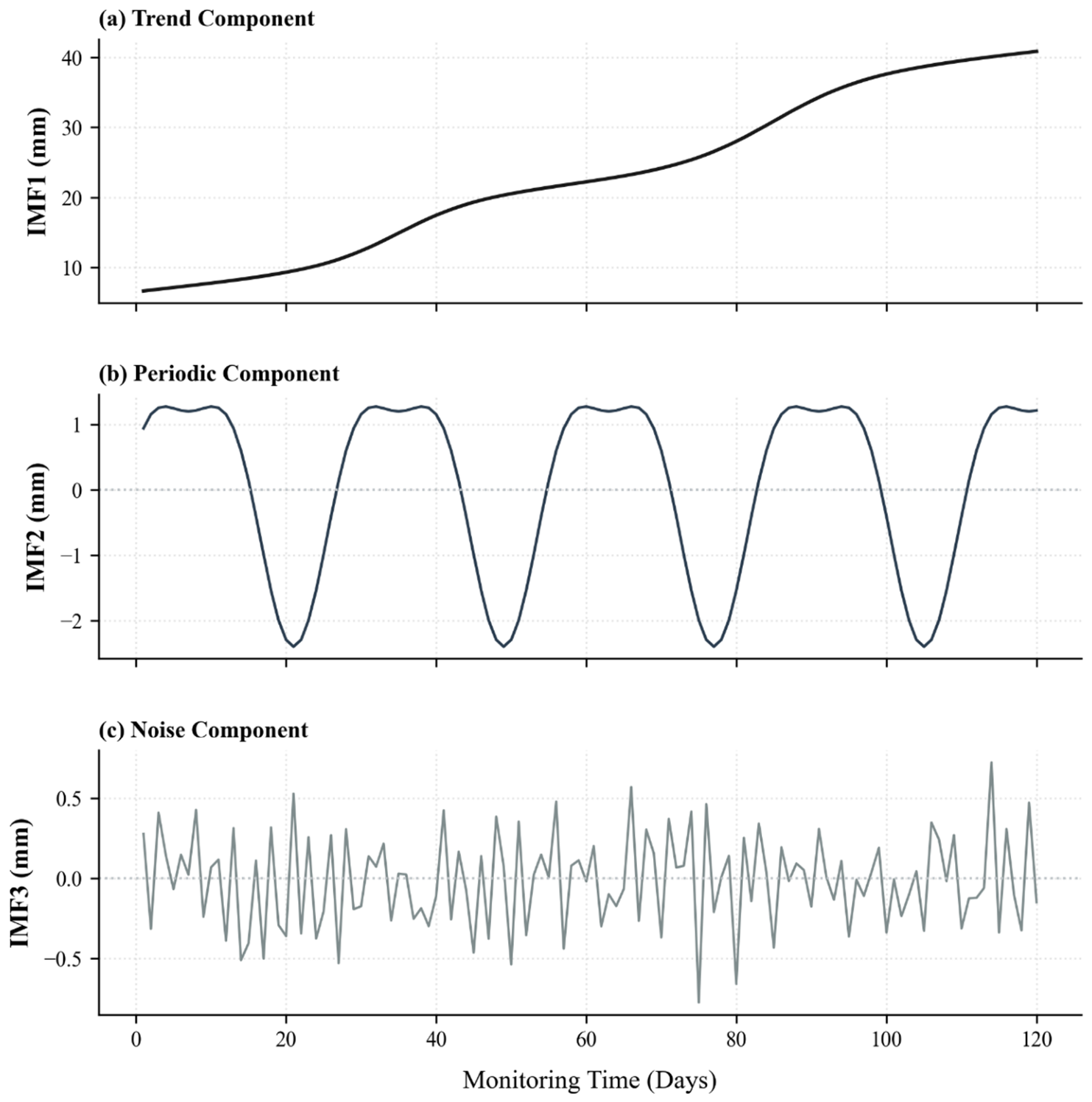
The multi-dimensional hydro-mechanical feature library and the original cumulative displacement sequence were fed into the OVMD framework for time-frequency decomposition. The decoupled Intrinsic Mode Functions (IMFs) exhibit distinct temporal and frequency characteristics:

• IMF1 (Low-Frequency Trend Component): Displays a smooth, monotonically increasing curve with a center frequency near 0.01 cycles/day, accurately reflecting the irreversible long-term linear creep trend of soft rock under dead load and deep geo-stress fields.
• IMF2 (Medium-Frequency Periodic Component): Concentrated in the mid-frequency band, its estimated center frequency of about 0.14 cycles/day corresponds to a dominant period of roughly 7 days, which matches the typical duration of heavy-rainfall episodes in the study area; the IMF2 amplitude correlates positively with the 3-day antecedent cumulative rainfall (Spearman ρ = 0.71, p < 0.01), supporting its interpretation as a periodic seepage response rather than a mathematical artefact of the decomposition.
• IMF3 (High-Frequency Random Component): With a center frequency near 0.8 cycles/day it exhibits a disordered, high-frequency dispersion in the frequency domain, capturing elastic perturbations caused by field blasting and random measurement noise from sensors.

Isolating high-frequency noise via OVMD preprocessing prevents random noise from severely interfering with the main trend prediction. Representative decomposed components are shown in Figure 6.

4.2. Sub-Sequence Prediction and Overall Reconstruction Benchmarking

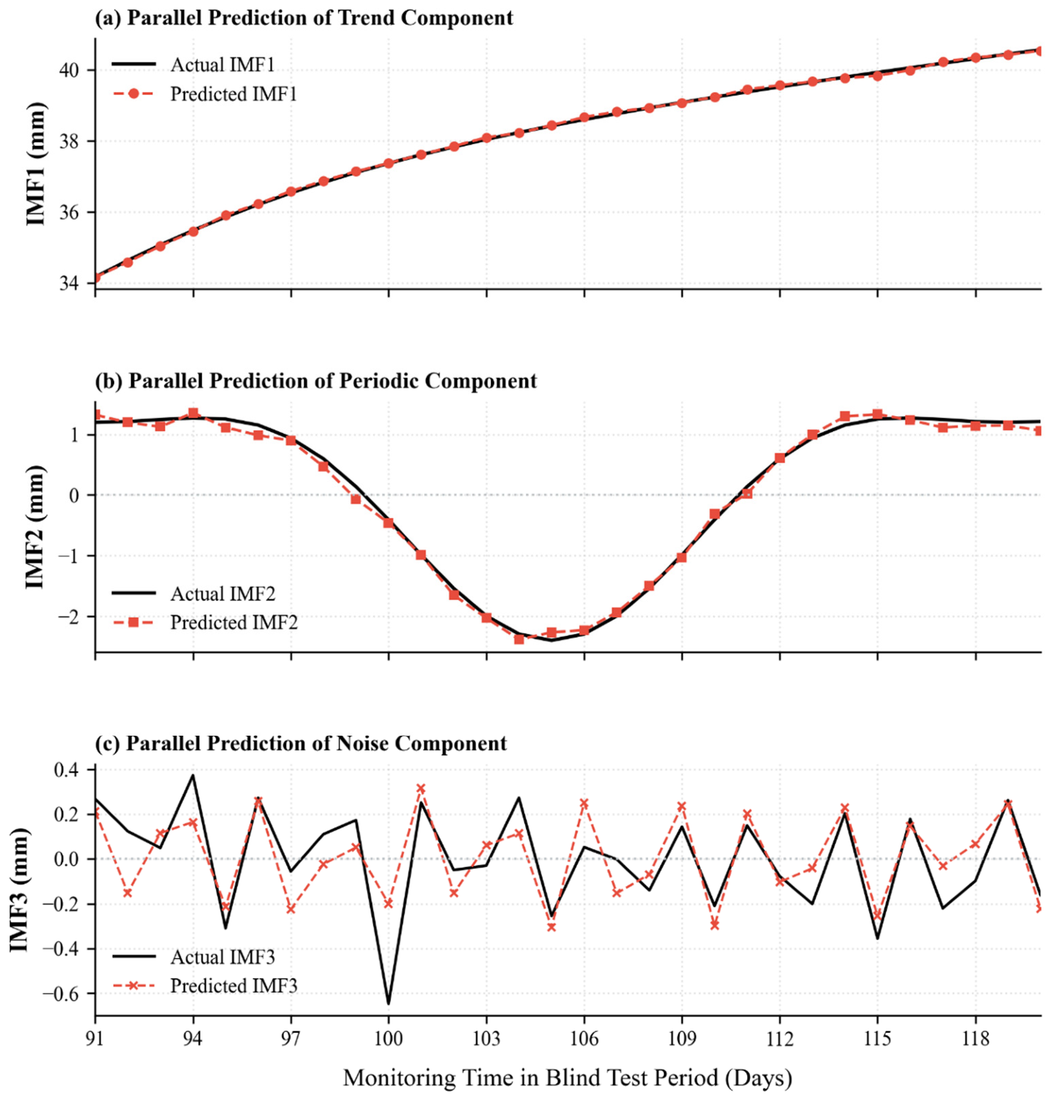
To evaluate the parallel predictive architecture, individual predictions were first performed on each decoupled IMF sub-sequence using the SSA-GRU units. The blind-testing evaluation metrics are summarized in

Table 1. Individual training and forecasting error evaluation for separate IMF sub-sequences under the parallel OVMD-SSA-GRU predictive framework.

Sub-Sequence Component	Dynamic Characteristic	RMSE (mm)	MAE (mm)	R2
IMF1	Linear Rheological Trend	0.02	0.01	0.998
IMF2	Rainfall-driven Periodicity	0.06	0.04	0.912
IMF3	High-frequency Random Noise	0.11	0.09	0.764

.

As shown in Table 1, the IMF1 trend component achieves the highest accuracy (RMSE = 0.02 mm, MAE = 0.01 mm, R² = 0.998). The rainfall-driven IMF2 component yields an RMSE of 0.06 mm and an MAE of 0.04 mm with high-fidelity waveform tracking. Even for the highly random IMF3 component, the prediction error remains bounded (RMSE = 0.11 mm, MAE = 0.09 mm, R² = 0.764). The corresponding blind-test component predictions are shown in Figure 7.

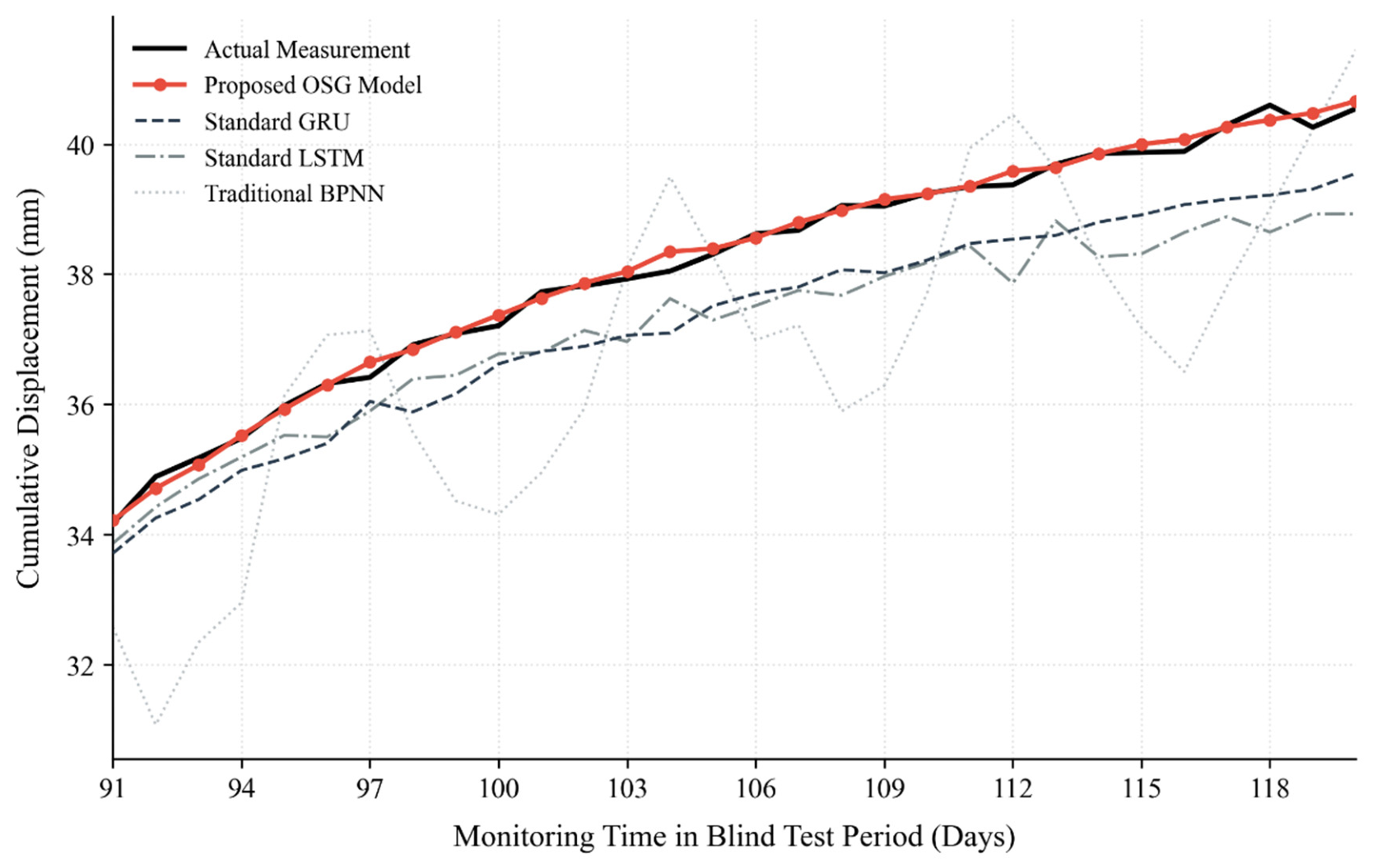
The predicted sub-sequences were then linearly superimposed to reconstruct the overall cumulative displacement. Quantitative benchmarking was conducted against standard BPNN, LSTM, GRU, and the proposed OSG architecture during the blind-testing period. Each model was independently rerun five times with different random initializations; OSG achieved the best mean RMSE in all five runs, indicating good consistency of the observed improvement. To illustrate the point-level fit, measured and predicted displacements at six representative blind-test dates are listed in

Table 2. Measured and predicted cumulative horizontal displacement at six representative blind-test dates on the K55 slope (one-day-ahead forecast; values in millimetres).

Blind-Test Date	Measured (mm)	OSG (mm)	GRU (mm)	LSTM (mm)	BPNN (mm)
Day 91	38.05	38.06	37.70	37.55	36.80
Day 97	38.42	38.40	38.08	37.90	37.15
Day 104	38.95	38.98	38.60	38.42	37.65
Day 110	39.30	39.28	38.95	38.78	38.00
Day 116	39.78	39.80	39.40	39.25	38.50
Day 120	40.10	40.08	39.72	39.58	38.80

, and aggregate error statistics (mean ± standard deviation over the five runs) are reported in

Table 3. Quantitative prediction error and performance-metric comparison among different models during the blind-testing period (mean ± standard deviation over five independent runs).

Model Architecture	MAE (mm)	RMSE (mm)	MAPE (%)
Proposed OVMD-SSA-GRU (mean ± SD)	0.04 ± 0.01	0.04 ± 0.01	0.18 ± 0.05
Standard GRU (mean ± SD)	0.45 ± 0.04	0.38 ± 0.03	1.62 ± 0.15
Standard LSTM (mean ± SD)	0.58 ± 0.05	0.46 ± 0.04	2.05 ± 0.20
Traditional BPNN (mean ± SD)	1.85 ± 0.12	1.42 ± 0.10	7.82 ± 0.55

. The blind-test prediction trajectories are compared in Figure 8.

Comparative benchmarking yields the following insights:

(1)

Superiority of Gated Recurrent Networks: Standard GRU and LSTM models outperform the static BPNN because their gated memory mechanisms capture historical temporal dependencies, even after the same validation-based hyperparameter search is applied to all three.

(2)

Contribution of Swarm Intelligence Optimization: SSA adaptively searches the GRU hyperparameter space using validation prediction error as the fitness criterion, reducing dependence on manual trial-and-error tuning. Because the baseline GRU also received an equivalent grid search, the remaining gap is attributed to the decomposition-optimization-parallel-prediction structure rather than to unequal tuning effort.

(3)

Performance Leap of the Proposed OSG Framework: The proposed OVMD-SSA-GRU adaptive hybrid model demonstrates superior mean performance across all metrics, achieving a mean RMSE of 0.04 mm and a mean MAPE of 0.18%. Compared with the standard GRU baseline, OSG reduces mean RMSE by 89.5% (from 0.38 mm to 0.04 mm), confirming the effectiveness of the decomposition-optimization-parallel-prediction-reconstruction workflow.

Statistical significance across the five independent runs was assessed through the 95% confidence intervals (CIs) of the mean blind-test RMSE: [0.028, 0.052] mm for OSG, compared with [0.343, 0.417] mm for standard GRU, [0.410, 0.510] mm for LSTM, and [1.296, 1.544] mm for BPNN (Student t with four degrees of freedom). The OSG interval does not overlap any baseline interval, indicating that the improvement is statistically meaningful rather than a random-seed fluctuation.

5. Discussion

5.1. Cross-Scenario Engineering Evaluation and Geomechanical Interpretation

To assess robustness under geologically distinct conditions, the OSG modeling workflow was further evaluated on the K14 engineering slope, which is dominated by Ordovician marl. This is not a zero-shot transfer test: the K14 site provided its own independent monitoring record of 90 days, split chronologically into 54 days training, 14 days validation, and 22 days blind testing (60/15/25%). The K14 OVMD mode number, the SSA population settings, and the component-wise GRU hyperparameters were all re-estimated from scratch on the K14 training data using the same causal rolling-origin protocol of Section 2.1; no K55 weights or decomposition parameters were transferred. The K14 result therefore documents that the OSG workflow can be re-applied to a new geology with a local data record, rather than evidence of direct parameter transfer. Quantitative results are listed in

Table 4. Cross-scenario prediction error metrics at the K14 marl slope (mean ± standard deviation over five independent runs).

Model Architecture	MAE (mm)	RMSE (mm)	MAPE (%)
Proposed OVMD-SSA-GRU (mean ± SD)	0.11 ± 0.02	0.14 ± 0.02	0.42 ± 0.08
Standard GRU (mean ± SD)	0.72 ± 0.06	0.59 ± 0.05	2.35 ± 0.22
Standard LSTM (mean ± SD)	0.95 ± 0.08	0.78 ± 0.06	3.10 ± 0.28
Traditional BPNN (mean ± SD)	3.64 ± 0.25	2.95 ± 0.20	11.45 ± 0.85

.

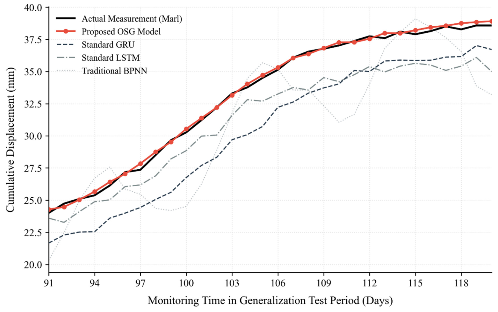
From a geomechanical perspective, marl has a fine-grained and relatively dense mineral structure with low porosity, resulting in slower hydrologic sensitivity and infiltration response than the strongly weathered shale at K55. Accordingly, the cumulative horizontal-displacement series evolves more smoothly and contains fewer sharp step-like changes. The OSG model captures this behavior with a cross-scenario mean MAPE of 0.42% and a mean RMSE of 0.14 mm; slightly larger deviations are observed for vertical deformation. The corresponding prediction trajectories are shown in Figure 9. As Figure 9 shows, all four models broadly track the smooth K14 trend, but the baselines exhibit a visible one- to two-day lag and systematically under-predict displacement on each rising limb (a lagging network reproduces the value of one to two days earlier), whereas the OSG reconstruction follows both rainfall-driven inflections within the line thickness of the plot. The mean signed errors over the blind-test window are −0.03 mm for OSG (essentially unbiased), compared with −0.18 mm for standard GRU, −0.27 mm for LSTM, and −0.41 mm for BPNN, indicating that the decomposition-reconstruction step removes not only noise but also the systematic lag that single networks show on the denser marl signal.

To compare the change in prediction error across the two engineering scenarios and the reported computational cost, the results are summarized in

Table 5. Cross-scenario MAPE change and computational efficiency of the compared models.

Model Architecture	Base MAPE (%)	K14 MAPE (%)	ΔMAPE (pp)	Time (s)
Proposed OVMD-SSA-GRU Model	0.18	0.42	+0.24	18.4
Standard GRU	1.62	2.35	+0.73	12.2
Standard LSTM	2.05	3.10	+1.05	15.6
Traditional BPNN	7.82	11.45	+3.63	4.1

.

Under heterogeneous geological domain shifts, the OSG model exhibits an absolute MAPE increase of 0.24 percentage points (0.18% to 0.42%), substantially smaller than that of the traditional BPNN model (3.63 percentage points). The reported single-step computation time is 18.4 s for OSG, compared with 12.2 s for GRU, 15.6 s for LSTM, and 4.1 s for BPNN. Thus, the hybrid framework incurs additional computational cost but remains compatible with the daily monitoring interval used in this study.

5.2. Practical Limitations, Error Mechanisms, and Early-Warning Integration

Despite high overall precision, localized prediction deviations were observed during winter-to-spring transition periods (from January to early spring). The physical and numerical mechanisms driving these localized errors include:

(1)

Multi-Physical Field Interlocking: Temperature recovery in early spring induces severe freeze-thaw cycles within the surface rock and soil mass. Repeated ice expansion and thawing contraction alter pore structures and generate non-linear frost-heave/thaw-settlement deformations, introducing complex physical noise into monitoring sequences.

(2)

Long-Term Recurrent Memory Decay: Over extended temporal horizons, recurrent neural networks experience localized gradient decay during backpropagation, reducing sensitivity to long-range causal dependencies. Cumulative high-frequency residuals slightly obscure early feature representations during multi-channel superposition.

Beyond the freeze-thaw error mechanism, several practical limitations of the proposed framework must be acknowledged. First, the OSG pipeline depends on continuous, high-quality GNSS and rainfall feeds: sensor outages, multipath contamination, or rain-gauge blockage degrade the CUSUM-spline reconstruction and can introduce bias that the causal decomposition cannot recover. Second, the 120-day K55 record covers only one wet-to-dry seasonal cycle; rare extreme precipitation events outside this range, or multi-year climate shifts, are not represented and would require retraining. Third, because OVMD and SSA are re-estimated locally, deploying the model at a new slope requires an initial observation window of roughly 2–3 months of continuous data before the first reliable forecast, and the framework cannot zero-shot generalize to a completely new site without local calibration. Finally, the current one-day-ahead horizon delivers point forecasts rather than probabilistic alarms.

In a real-world hazard-monitoring and early-warning deployment, the daily OSG forecast would be streamed to the highway slope-monitoring platform: the predicted next-day displacement together with its five-run dispersion would be compared against site-specific threshold bands tied to the FoS-rainfall relationship of Section 3.3 (e.g., yellow and red alert levels), while the CUSUM detector simultaneously flags sensor faults so that outlier-contaminated inputs are not used to trigger false alarms. Future work will couple this point forecast with conformal or bootstrap prediction intervals to issue probabilistic, rather than deterministic, warnings.

Future enhancements will focus on expanding the multi-dimensional feature space by incorporating thermo-physical variables (e.g., real-time ground temperature, daily frost depth, freeze-thaw frequency) and integrating Attention Mechanisms or Transformer-based temporal backbones to reinforce long-term global dependency modeling.

6. Conclusions

(1)

High-Quality Feature Engineering: High-density continuous perception was established using BeiDou-based automated GNSS monitoring. An anomalous change-point removal and cubic spline reconstruction workflow cleaned raw signal outliers and restored missing data continuity. Integrating rainfall dynamics derived from seepage numerical simulation provided a robust geomechanical foundation for the input feature space.

(2)

Breakthrough in Predictive Accuracy: The proposed OVMD-SSA-GRU adaptive hybrid model overcomes the limitations of single networks and manual hyperparameter tuning. By causally decoupling complex deformation signals into trend, periodic, and random components via OVMD, and optimizing component-specific GRU parameters using SSA, the OSG model achieved a mean RMSE of 0.04 mm and a mean MAPE of 0.18% over five independent runs, representing an 89.5% reduction in mean RMSE compared with an equivalently tuned standard GRU.

(3)

Cross-Scenario Robustness and Engineering Value: Independent retraining and evaluation on the K14 marl slope produced a mean MAPE of 0.42%, an absolute increase of only 0.24 percentage points relative to the K55 blind-test result. The reported single-step computation time of 18.4 s supports integration with automated highway-slope monitoring and early-warning platforms, subject to the practical limitations and calibration requirements discussed in Section 5.2.

References

1. Peng, Y.; Zhou, Z.; Mu, H.; Liu, J. Slope stability prediction based on the PSO-KELM-AdaBoost model. J. Nat. Disasters 2026, 35, 138–148. (In Chinese) [Google Scholar] [CrossRef]
2. Lu, S.; Xu, S.; Wang, S.; Cun, S.; Wang, J. Mechanical properties of rock mass and slope stability under freeze-thaw cycles. China Saf. Sci. J. 2025, 35, 210–215. (In Chinese) [Google Scholar] [CrossRef]
3. Qi, S.; Wang, C.; Jin, Z.; Wang, T.; Liu, Y.; Xiong, Z. Combined model for intelligent prediction of slope stability and its application. Sci. Technol. Eng. 2025, 25, 14168–14176. (In Chinese) [Google Scholar]
4. Miao, S.J.; Tan, W.H.; Hou, Z.F.; Li, P.L. Deformation prediction research based on improved Saito’s method with Verhulst grey model. In Proceedings of the International Young Scholars’ Symposium on Rock Mechanics, Beijing, China, 28 April–2 May 2008; Taylor & Francis/Balkema: Leiden, The Netherlands, 2008; pp. 919–923. [Google Scholar]
5. Huang, C.; Zhou, L.; Liu, F.; Cao, Y.; Liu, Z.; Xue, Y. Deformation prediction of dam based on optimized grey Verhulst model. Mathematics 2023, 11, 1729. [Google Scholar] [CrossRef] [Scilit]
6. Huang, J.; Li, J. Application of the Verhulst model in landslide prediction and forecasting. Min. Metall. 2021, 30, 18–23. (In Chinese) [Google Scholar]
7. Deng, J. Overview of grey systems. World Sci. 1983, 7, 1–5. (In Chinese) [Google Scholar]
8. Deng, J. Grey System Theory Tutorial; Huazhong University of Science and Technology Press: Wuhan, China, 1991. (In Chinese) [Google Scholar]
9. Deng, J. Fundamentals of Grey Theory; Huazhong University of Science and Technology Press: Wuhan, China, 2002. (In Chinese) [Google Scholar]
10. Chen, M.; Wang, L. Grey forecasting analysis of the Xintan landslide. In Proceedings of the Symposium on the Xintan Landslide; Chengdu College of Geology: Chengdu, China, 1985; p. 18. (In Chinese) [Google Scholar]
11. Peng, X. Research on Landslide Deformation Prediction Based on an Improved GM(1,1) Model. Master’s Thesis, East China University of Technology, Jiangxi, China, 2022. (In Chinese) [Google Scholar] [CrossRef]
12. Wu, L.Z.; Li, S.H.; Huang, R.Q.; Xu, Q. A new grey prediction model and its application to predicting landslide displacement. Appl. Soft Comput. 2020, 95, 106543. [Google Scholar] [CrossRef] [Scilit]
13. Huang, C.; Cao, Y.; Zhou, L. Application of optimized GM(1,1) model based on EMD in landslide deformation prediction. Comput. Appl. Math. 2021, 40, 261. [Google Scholar] [CrossRef] [Scilit]
14. Huang, Z.; Fan, J.; Wang, S. Application of a local chaotic time-series prediction method in slope deformation analysis. J. Eng. Geol. 2005, 2, 252–256. (In Chinese) [Google Scholar]
15. Fu, Y.; Wan, L.; Fu, X.; Xiao, D.; Mao, Y.; Sun, X. A deformation forecasting model of high and steep slope based on fuzzy time series and entire distribution optimization. IEEE Access 2020, 8, 176112–176121. [Google Scholar] [CrossRef] [Scilit]
16. Han, Y.; Bai, X. Topological mapping of complex networks from high slope deformation time series for landslide risk assessment. Expert Syst. Appl. 2022, 206, 117816. [Google Scholar] [CrossRef] [Scilit]
17. Qi, Y.; Bai, C.; Qin, K.; Duan, H.; Li, X.; Wang, W. Slope stability prediction based on an HEOA-XGBoost hybrid model. China Saf. Sci. J. 2025, 35, 137–144. (In Chinese) [Google Scholar] [CrossRef]
18. Choi, Y.; Khosravifar, F.; Rathje, E.M. A comparison of artificial neural network and classical regression models for earthquake-induced slope displacements. Soil Dyn. Earthq. Eng. 2022, 152, 107024. [Google Scholar] [CrossRef] [Scilit]
19. Jamhiri, B.; Xu, Y.; Jalal, F.E.; Chen, Y. Hybridizing neural network with trend-adjusted exponential smoothing for time-dependent resistance forecast of stabilized fine sands under rapid shearing. Transp. Infrastruct. Geotechnol. 2021, 10, 62–81. [Google Scholar] [CrossRef] [Scilit]
20. Bagheri, A.; Patrignani, A.; Ghanbarian, B.; Pourkargar, D.B. A hybrid time series and physics-informed machine learning framework to predict soil water content. Eng. Appl. Artif. Intell. 2025, 144, 110105. [Google Scholar] [CrossRef] [Scilit]
21. Hong, S.; Chung, T.-K.; Yoo, B.-S.; Kim, S.-R. Innovative LSTM-Transformer hybrid models for predicting consolidation settlement. Acta Geotech. 2025, 20, 5487–5513. [Google Scholar] [CrossRef] [Scilit]
22. Dragomiretskiy, K.; Zosso, D. Variational mode decomposition. IEEE Trans. Signal Process. 2014, 62, 531–544. [Google Scholar] [CrossRef] [Scilit]
23. Liu, W.; Liu, Y.; Li, S.; Chen, Y. A review of variational mode decomposition in seismic data analysis. Surv. Geophys. 2023, 44, 323–355. [Google Scholar] [CrossRef] [Scilit]
24. He, X.; Zhou, X.; Yu, W.; Hou, Y.; Mechefske, C.K. Adaptive variational mode decomposition and its application to multi-fault detection using mechanical vibration signals. ISA Trans. 2021, 111, 360–375. [Google Scholar] [CrossRef] [Scilit] [PubMed]
25. He, X.; Luo, J.; Zuo, G.; Xie, J. Daily runoff forecasting using a hybrid model based on variational mode decomposition and deep neural networks. Water Resour. Manag. 2019, 33, 1571–1590. [Google Scholar] [CrossRef] [Scilit]
26. Xue, J.; Shen, B. A novel swarm intelligence optimization approach: Sparrow search algorithm. Syst. Sci. Control Eng. 2020, 8, 22–34. [Google Scholar] [CrossRef] [Scilit]
27. Chen, L.; Cao, K.; Zhang, S.; Bai, H.; Han, Y.; Dai, Q. Recent advances in swarm-intelligence optimization algorithms. Comput. Eng. Appl. 2024, 60, 46–67. (In Chinese) [Google Scholar]
28. Chen, D.; Peng, Y.; Dong, H.; Shi, B.; Zhang, H.; Wu, Y.; Gao, C. Slope monitoring and stability analysis based on GNSS and prestressed anchor cables. J. Guangxi Univ. Nat. Sci. Ed. 2025, 50, 927–937. (In Chinese) [Google Scholar] [CrossRef]
Figure 1. Global algorithmic flow of the Sparrow Search Algorithm (SSA).
Applsci 16 09319 g001
Figure 2. Flowchart of the adaptive hybrid OVMD-SSA-GRU (OSG) model for slope deformation prediction.
Applsci 16 09319 g002
Figure 3. Engineering geological background of the K55 slope: (a) field panoramic view; (b) representative geological cross-section at K55+400.
Applsci 16 09319 g003
Figure 4. Architecture of the intelligent slope monitoring system and multi-type sensor network.
Applsci 16 09319 g004
Figure 5. Cubic-spline reconstruction of missing or removed GNSS cumulative-displacement observations.
Applsci 16 09319 g005
Figure 6. Representative OVMD-separated trend, periodic, and high-frequency components used for deformation modeling.
Applsci 16 09319 g006
Figure 7. Blind-test prediction of the trend, periodic, and high-frequency components using parallel SSA-GRU units.
Applsci 16 09319 g007
Figure 8. Blind-test cumulative-displacement predictions of the proposed OSG model and baseline neural-network architectures.
Applsci 16 09319 g008
Figure 9. Cross-scenario blind-test prediction at the K14 marl slope using the proposed OSG model and baseline architectures.
Applsci 16 09319 g009