Conditional Deep Convolutional GAN for the Design of High-Performance Periodic Absorber Metasurfaces

Abstract

This work presents a conditional deep convolutional generative adversarial network (CDCGAN) for the inverse design of high-absorptance periodic metasurfaces (MSs) with different geometries. The conditioning mechanism encodes geometric and spectral parameters. A key innovation is the inclusion of unit cells with different periods to produce fine-tuned responses within the W-band. The period is embedded in the fringe pixels before training and recovered from generated high-resolution images to reconstruct the unit cell. This joint topology–period representation allows both the metallic geometry and lattice scale to be recovered from a single generative output without requiring a separate period-optimization stage. The resulting spectra closely matched the targets when tested at three angles of incidence, thereby demonstrating the method’s effectiveness for high-performance MS design.

1. Introduction

Metasurfaces (MSs) manipulate electromagnetic waves to achieve specific functionalities through sub-wavelength unit cells [1,2,3,4,5]. Though promising, their design is difficult due to the intricate relationships between geometries, materials and spectral response [6]. Designing MSs while optimizing local unit cells introduces complexity [7], requiring the solution of both forward and inverse electromagnetic problems [6,8,9]. Moreover, flat electromagnetic absorbers, whether single- or multilayered structures, selectively absorb electromagnetic waves [10], enabling diverse applications that require high-absorptance performance [11,12,13,14]. Though beneficial, their design demands extensive optimizations to obtain precise unit cells [11]. For this reason, AI-driven methods are emerging to address these limitations [15,16,17].

Conventional neural networks have been used to design MSs [18,19,20,21]. Generative adversarial network (GAN) models have been used for the inverse design of reflective polarizing MSs [9]. To add auxiliary parameters to the training process, Conditional GANs (CGANs) have been introduced to solve for transmissive MSs [22,23]. Meanwhile, variational autoencoders have been used for the forward design of reflective MSs [24], while related latent-space generative approaches have been combined with predictive regression networks for multilayered MSs [16]. To design high-absorption MSs, GANs were tested on Jerusalem-cross shapes [25,26], while multilayered absorbers were approached using autoencoders [24,27]. Deep learning algorithms were also tested to generate non-canonical absorbing MSs by employing binary-encoded unit cells [28].

This work presents a conditional deep convolutional GAN (CDCGAN) [29] for the inverse design of absorbing MSs in the W-band (75–78 GHz). While deep learning has been extensively applied to MSs absorber design, our work introduces novel contributions that directly address practical challenges and enhance the design process.

This work focuses on the representation adopted for periodic metasurface inverse design. In addition to the local metallic topology, the global lattice period is embedded in reserved fringe pixels of the same high-resolution image. The generator produces a joint topology–period representation from which both the metallic geometry and the physical unit-cell scale can be recovered. We introduce the following: (i) An early conditioning scheme that concatenates the spectral target and geometry class before the first dense layer, yielding fast convergence and high fidelity. (ii) A period-in-fringe encoding scheme that embeds the unit-cell size into image pixels and learns it jointly with the metallic topology. The generated fringe therefore provides the lattice scale associated with a particular generated sample, allowing both the topology and the period to be recovered from the same image representation produced by the generator for a given target spectrum. This enables variable-period generation within the range represented by the training data without requiring a separate period-optimization step, (iii) High-resolution, simulation-ready images that are suitable for wavelength-scale designs and interface directly with commercial full-wave solvers (HFSS). The generated image is post-processed to recover the encoded period and metallic contour and to produce the corresponding DXF files for 3D modeling and full-wave reconstruction. Thus, the proposed workflow avoids a separate iterative geometry-optimization stage after generation. A practical advantage of this approach is that the lattice period is generated together with the topology, rather than chosen a priori. The period strongly influences the resonance and cannot be uniquely inferred from the target spectrum [30], so it is conventionally selected by trial-and-error, whereas here it is treated as a learned design variable jointly produced by the CDCGAN. Because the electromagnetic inverse problem is generally non-unique, the proposed framework does not assume that a target absorptance spectrum uniquely determines the lattice period. Rather, the conditional generator produces one geometry–period realization from the distribution learned from the training data. Thus, the period-in-fringe encoding provides an explicit representation of the lattice scale associated with the generated sample, rather than imposing a unique spectrum-to-period mapping. Finally, we validated a generated unit cell experimentally, obtaining close spectral agreement at three different incidence angles.

2. Architecture and Training

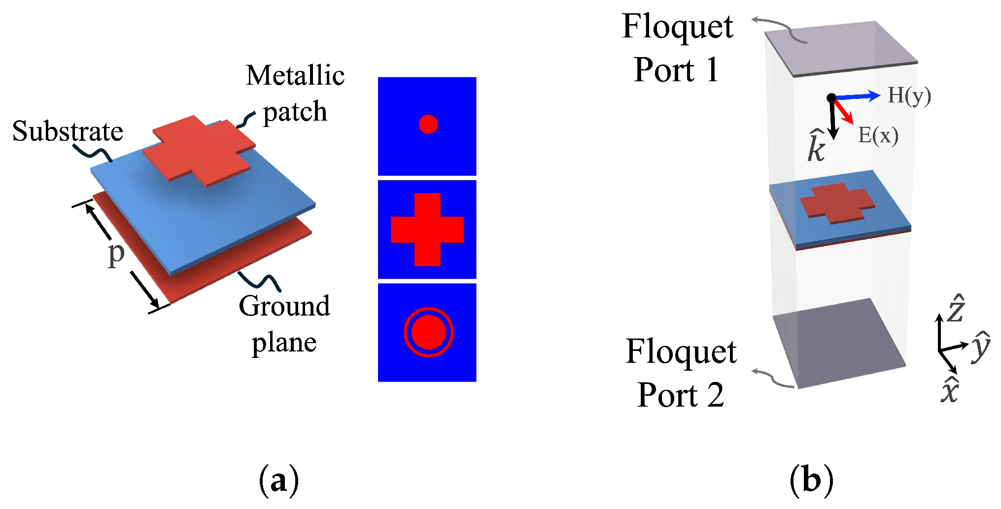
We start with three canonical shapes of the absorbing unit cells, as presented in Figure 1a. Each cell consists of a grounded Rogers 5880 substrate of thickness $d=0.508$ mm, a period p, and a metallic patch etched on top. The simulations were conducted in Ansys HFSS 2025 R1 with Floquet ports to evaluate MS responses, using a configuration as depicted in Figure 1b. To improve the relevance of the model, the training targets are high-absorptance responses in the 75–78 GHz band, thus requiring variations in both metallic patches and periods.

A Python 3.13.0 script was used to construct the electromagnetic database by randomly varying the geometric parameters of the unit cells, including the lattice period, radii, lengths, widths, and separations, within predefined constraints. The final curated dataset used for this study contains 20,543 simulated image–spectrum pairs distributed among three canonical geometries: circular, cross-shaped, and ring-shaped unit cells (see

Table 1. Distribution of the dataset used for CDCGAN training and validation.

Geometry	Number of Samples	Fraction (%)
Circular	6116	29.8
Cross	8000	38.9
Ring	6427	31.3
Total	20,543	100.0

). The original simulation pool contained a larger number of cross-shaped examples. To reduce the class imbalance, this class was downsampled to 8000 samples before constructing the final training dataset. Each full-wave simulation required approximately 5–8 min, corresponding to approximately 1660 h of cumulative electromagnetic simulation time. Prior to training, $15\%$ of the available samples were held out from gradient-based optimization and used for validation and testing, divided into training, validation, and independent test subsets using approximately $85\%$, $10\%$, and $5\%$ of the available samples, respectively. For the 20,543 samples used in the reported dataset, this corresponds to approximately 17,461 training samples, 2055 validation samples, and 1027 test samples. The training subset was used for gradient-based network optimization, whereas the validation subset was used to monitor training and select the final model configuration. The independent test subset was reserved exclusively for final evaluation.

The absorptance is extracted from the simulated scattering parameters for the TM and TE polarizations, according to Equations (1) and (2) [31]. A top-view of the model is saved to serve as training input, encoding physical layers, namely, the metallic patch (red) and the substrate (blue).

$${\mathrm{Abs}}_{\mathrm{TM}}=1-\mid S_{21}^{\mathrm{TM}}{\mid }^2-\mid S_{11}^{\mathrm{TM}}{\mid }^2$$

(1)

$${\mathrm{Abs}}_{\mathrm{TE}}=1-\mid S_{21}^{\mathrm{TE}}{\mid }^2-\mid S_{11}^{\mathrm{TE}}{\mid }^2$$

(2)

Both TE- and TM-polarized responses can be extracted from the full-wave simulations. However, only the TE-polarized absorptance spectra at normal incidence, $\theta =0^{\circ }$, were used as spectral inputs during CDCGAN training. The TM response was not used as a training target in the present model. For the canonical geometries considered here, the symmetry of the unit cells leads to similar TE and TM responses under the illumination conditions studied. For geometries exhibiting polarization-dependent behavior, however, the TM response could be used to train a separate polarization-specific network.

During pre-processing, all training images were resized to $512\times 512$ pixels to provide high-resolution input to the model. Additionally, the unit-cell period p, ranging from 4.85 to 5.3 mm, was linearly rescaled to the $[-1,1]$ range and embedded into the fringe pixels, thereby preserving pixel integrity. At inference time, the lattice period does not need to be specified a priori; instead, the generator produces an image containing both the metallic topology and the encoded lattice scale, from which the period is subsequently recovered. Thus, within the period domain represented by the training data, variable-period unit cells can be generated without requiring an independently prescribed period or a separate post-generation period-optimization step. The electromagnetic inverse problem is generally non-unique; therefore, the proposed model does not assume that a target absorptance spectrum uniquely determines the unit-cell period p. Instead, let $x_c=[\mathcal{L},\mathcal{C}]$ denote the complete conditioning input, comprising the target absorptance spectrum $\mathcal{L}$ and the auxiliary conditioning vector $\mathcal{C}$. For each generation, a 400-dimensional latent vector $\mathcal{Z}$ is sampled from a standard multivariate normal distribution,

$$\mathcal{Z}\sim p_{\mathcal{Z}}\left(\mathcal{Z}\right)=\mathcal{N}\left(0,I_{400}\right),$$

(3)

and the trained generator produces a corresponding RGB image, $\hat{\mathcal{I}}=G_{\mathit{\varphi }}\left(x_c,\mathcal{Z}\right)$, where $G_{\mathit{\varphi }}$ denotes the generator parameterized by the learned network weights $\mathit{\varphi }$ and $\hat{\mathcal{I}}$ is the generated $512\times 512\times 3$ image. The metallic topology and lattice period are subsequently recovered from this image through the deterministic post-processing operation

$$\left(\hat{\mathcal{G}},\hat{p}\right)=\mathrm{Dec}\left(\hat{\mathcal{I}}\right),$$

(4)

where Dec denotes the image-decoding and geometry-reconstruction procedure, $\hat{\mathcal{G}}$ is the recovered metallic topology, and $\hat{p}$ is the period decoded from the image fringe. The fringe therefore does not impose uniqueness on the inverse problem; rather, it provides an explicit representation of the lattice period associated with a particular generated sample.

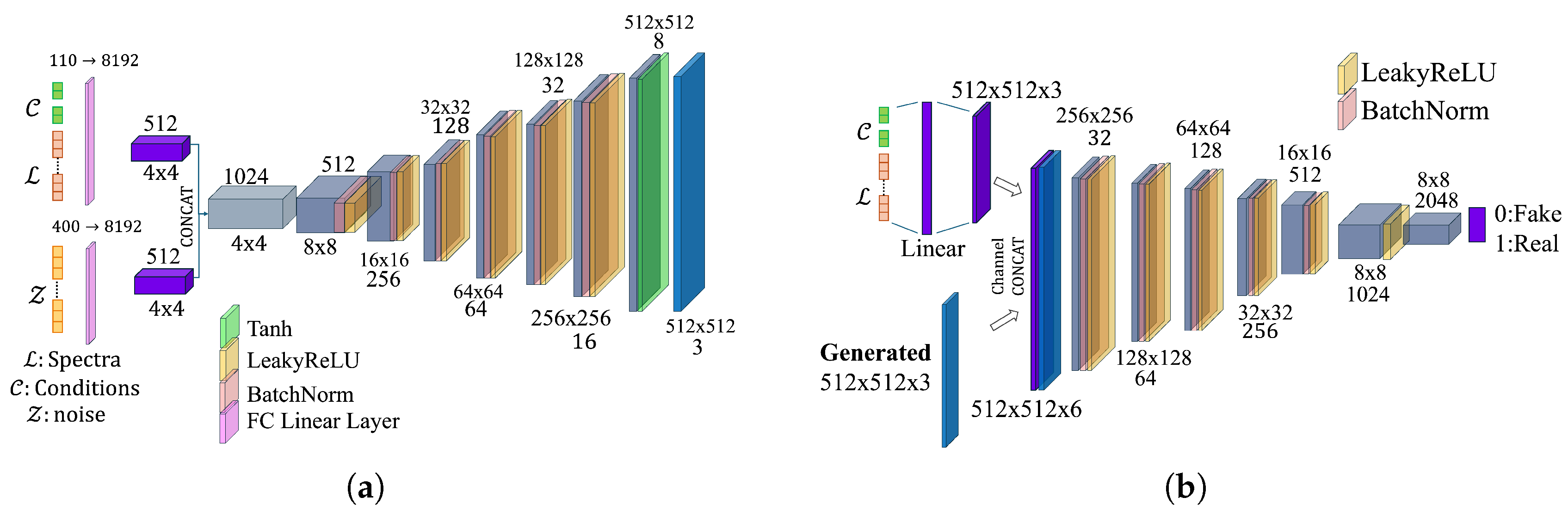
The CDCGAN follows a GAN architecture [29,32], with a generator producing realistic $512\times 512\times 3$-pixel unit-cell images from target absorptance spectra and conditioning data, and the discriminator assesses their authenticity (see Figure 2a,b). Detailed architectures, including layer and filter configurations, are shown in Figure 2. The training input consisted of TE-polarization absorptance spectra $\mathcal{L}$ with 100 frequency samples, a conditioning vector $\mathcal{C}$, and a latent noise vector $\mathcal{Z}$. 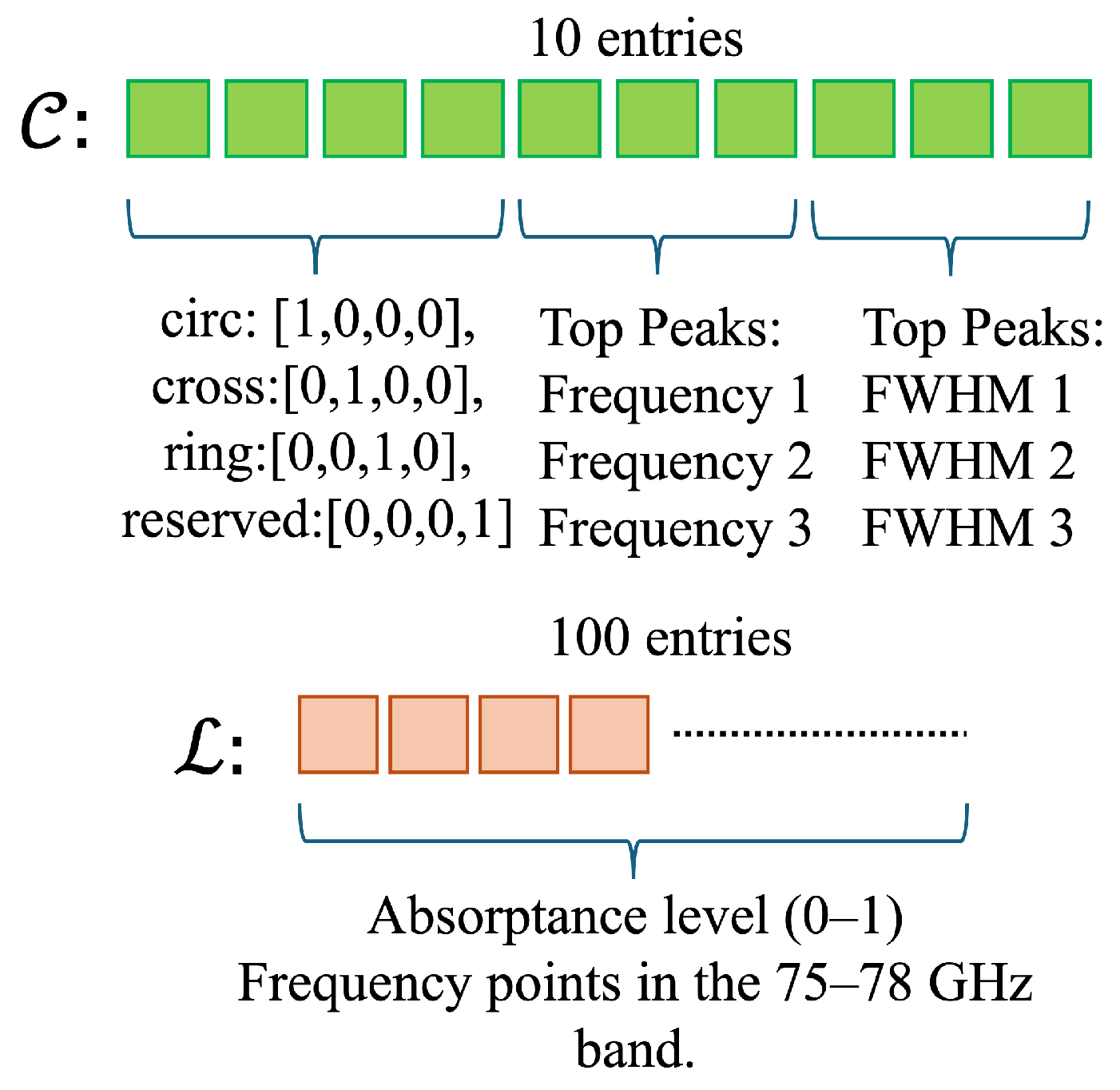The vector $\mathcal{C}$ encodes the unit-cell shape using a one-hot representation for circle, cross, and ring classes, and can include additional parameters, as presented in Figure 3. Furthermore, $\mathcal{C}$ is concatenated with the absorptance spectrum vector $\mathcal{L}$.

The resulting conditioning vector, with 110 entries, is mapped by a fully connected layer to 8192 features and then reshaped as a $4\times 4\times 512$ tensor. Independently, the latent vector $\mathcal{Z}\in {\mathbb{R}}^{400}$ is projected to 8192 features and reshaped to a second $4\times 4\times 512$ tensor. Concatenation along the channel dimension yields a $4\times 4\times 1024$ tensor, which is supplied to the first transposed-convolution block of the generator. This integration occurs before the input is passed through the first dense layer, ensuring that conditioning information is embedded from the earliest stage of the generation process. Though this model targets single-band absorbers, its structure supports future extension to dual-band responses. For this reason, the top three absorptance peaks and their full width at half maximum (FWHM) are extracted from ground-truth and included in $\mathcal{C}$, thus enabling the model to learn more spectral features. The detailed layer-by-layer architecture of the generator and discriminator is summarized in

Table 2. Layer-by-layer architecture of the CDCGAN generator and discriminator. K, S, and P denote kernel size, stride, and padding, respectively.

Stage	Operation	In Ch.	Out Ch.	K	S	P
Generator
G1	ConvTranspose2d	1024	512	5	1	0
G2	ConvTranspose2d	512	256	6	2	2
G3	ConvTranspose2d	256	128	6	2	2
G4	ConvTranspose2d	128	64	6	2	2
G5	ConvTranspose2d	64	32	6	2	2
G6	ConvTranspose2d	32	16	6	2	2
G7	ConvTranspose2d	16	8	6	2	2
G8	ConvTranspose2d	8	3	5	1	2
Discriminator
D1	Conv2d	6	32	6	2	4
D2	Conv2d	32	64	6	2	5
D3	Conv2d	64	128	6	2	4
D4	Conv2d	128	256	6	2	2
D5	Conv2d	256	512	6	2	2
D6	Conv2d	512	1024	6	2	2
D7	Conv2d	1024	2048	2	2	1
D8	Conv2d	2048	1	6	2	1

.

Both networks used ADAM optimizers with ${\beta }_1=0.8$ and ${\beta }_2=0.999$. To improve stability, one-sided label smoothing was applied to real and fake labels [33], and random label flipping was introduced to prevent discriminator overconfidence [34]. Regularization through exponential learning rate decay further enhanced generalization.

A hyperparameter optimization was employed to maximize the similarity between validation and generated images. To assess shape similarity between reference and generated images, denoted $A=[a_1,\dots ,a_n]$ and $B=[b_1,\dots ,b_n]$, where A and B are flattened images, the cosine similarity (CS) is considered as in Equation (5). The CS metric ranges from $-1$ to 1, with 1 indicating identical direction, 0 denotes orthogonality, and $-1$ signifies opposite directions [35].

$$\mathrm{Cosine}\mathrm{Similarity}={\displaystyle \frac{{\sum }_{i=1}^n{a}_i{b}_i}{\sqrt{{\sum }_{i=1}^n{a}_i^2}\sqrt{{\sum }_{i=1}^n{b}_i^2}}}$$

(5)

To further confirm the similarity between both images, the structural similarity index measure (SSIM) is used. The SSIM measures geometric precision, enhancing the model’s reliability. For two image patches x and y, SSIM is defined in Equation (6). Here, ${\mu }_x$, ${\mu }_y$ are the mean intensities, ${\sigma }_x^2$, ${\sigma }_y^2$ are the variances, and ${\sigma }_{xy}$ is the covariance. The constants $C_1={\left(k_{1}L\right)}^2$ and $C_2={\left(k_{2}L\right)}^2$ stabilize the division, with L being the dynamic range of the pixel values, and typical values $k_1=0.01$, $k_2=0.03$. We use the torchmetrics package to compute the SSIM between reference and generated images [36].

$$\mathrm{SSIM}(x,y)={\displaystyle \frac{(2{\mu }_x{\mu }_y+C_1)(2{\sigma }_{xy}+C_2)}{({\mu }_x^2+{\mu }_y^2+C_1)({\sigma }_x^2+{\sigma }_y^2+C_2)}}$$

(6)

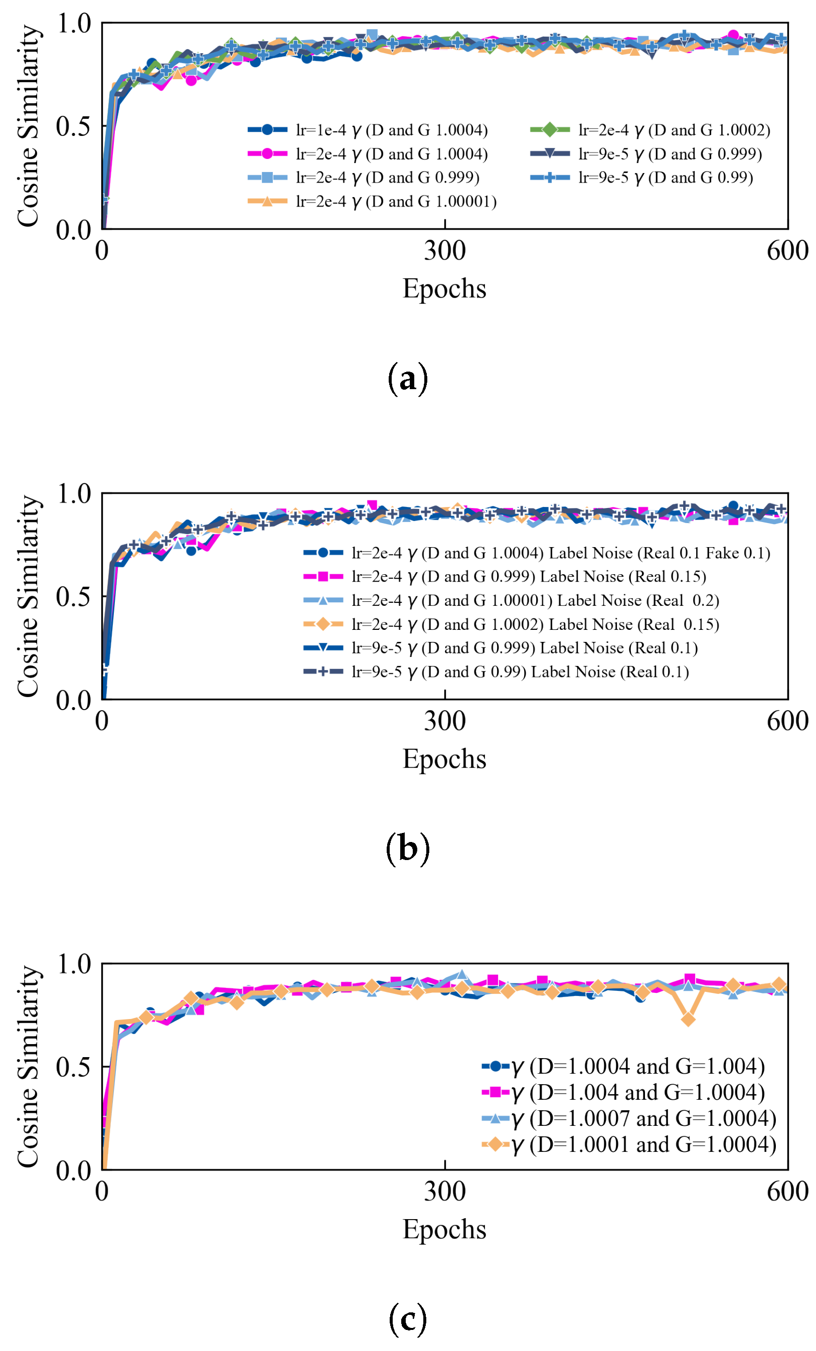
The sensitivity of our model was optimized against the CS metric, tuning key hyperparameters with the aim of quantifying effects on generation quality. We investigated different learning rate values, exploring three particular values: 0.0001, 0.0002 (default), 0.00009. As shown in Figure 4a, the learning rate of 0.0002 resulted in the most stable convergence and the highest CS values, without incurring overfitting. For instance, moving from 0.0001 to 0.0002 in our learning rate increased the CS from 0.86 up to 0.92. Moreover, after several tests, we settled on a latent dimension of 400 to provide the best trade-off between convergence speed and generation quality. A lower dimension reduced sample diversity, thus leading to repetitive patterns, while a higher dimension slowed training and resulted in less stable convergence. Also, to improve generalization and reduce discriminator overconfidence and memorization, we use one-sided label smoothing together with random label flipping, effectively introducing label noise during training. We tested noise levels of 0%, 10%, and 20%, and found that 10% provided the best validation performance, improving stability while preserving a clear separation between real and generated samples (Figure 4b). Finally, we also studied the effect of exponential learning rate decay by tuning the gamma parameter. As shown in Figure 4c, we tested gamma values in the range of [0.99, 1.0004]. A decay factor of $\gamma$ = 0.99 provided the most stable training curve while slightly improving final reconstruction accuracy. Gamma values $<0.9$ decayed the learning rate too rapidly, thus preventing convergence.

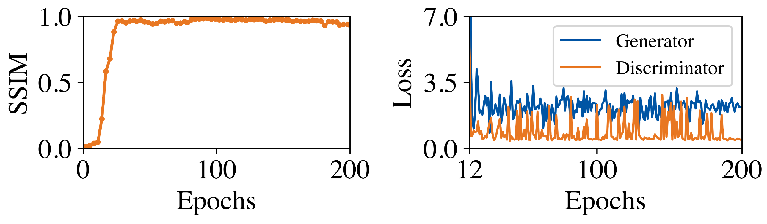
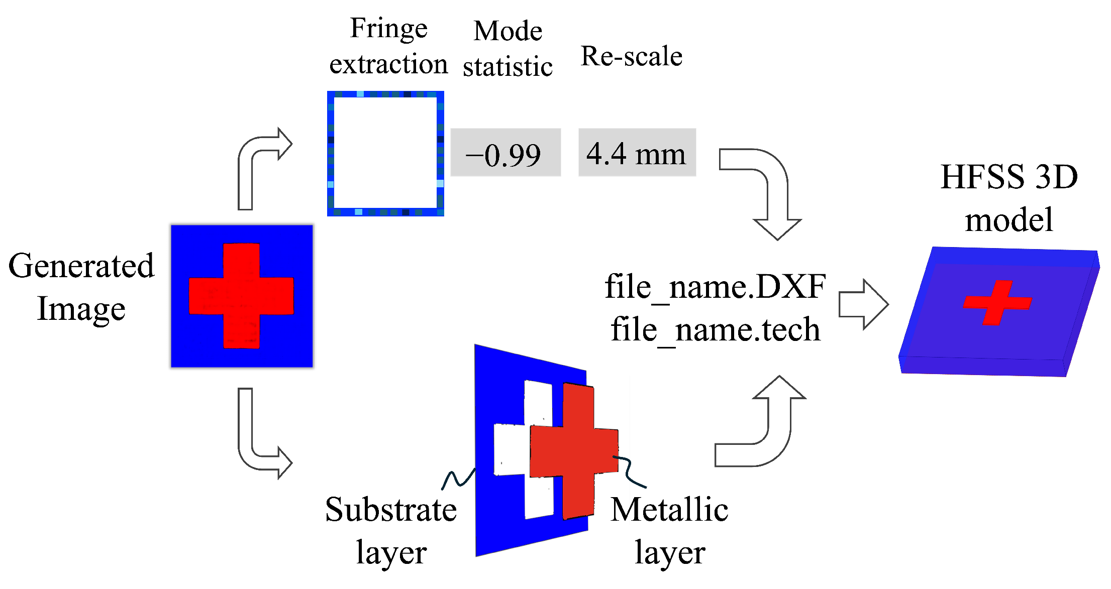
Figure 5 shows the evolution of the SSIM during training, comparing generated cells with their references; the improved fidelity is associated with fewer geometry-induced features in later simulations. The training was conducted on two NVIDIA H100 GPUs for 200 epochs with a batch size of 64, exhibiting expected adversarial dynamics (see Figure 5). The full training process took ∼21 h to complete. After training, generated images undergo post-processing for simulation (Figure 6). The period is recovered from the blue channel’s fringe by inverse-mapping from $[-1,1]$ to the original scale. Images are converted to HSV via OpenCV, and binary masks isolate substrate and metallic patches. Contours from the masks are processed by a Python module to produce .DXF and .tech files for HFSS. Validation simulations are used to confirm that the generated unit cells match the target absorptance spectra. Thus, although an automated geometry-reconstruction stage is required, the proposed workflow avoids a separate iterative geometry-optimization stage after generation. Finally, generating a new unit cell and running the post-processing pipeline takes 8 s per sample, enabling the integration with full-wave verification.

3. Results and Discussion

Generation batches were carried out using reference spectra randomly sampled from the test dataset. The unit cell was generated using the normal-incidence conditioning input; incidence angle was not included in the CDCGAN conditioning vector. All samples were generated successfully, matching the target shape. We evaluated spectral and geometric fidelity using three metrics for a rigorous comparison. The agreement between ground-truth and generated absorptance curves is quantified by mean squared error (MSE) and CS metrics, confirming the model’s accuracy. MSE measures the error between two curves, with lower values indicating a closer match [37]. For curves represented by vectors $X=[x_1,\dots ,x_n]$ and $Y=[y_1,\dots ,y_n]$, where n is the number of data points, the MSE is defined as in Equation (7).

$$\mathrm{MSE}={\displaystyle \frac{1}{n}}{\displaystyle \sum _{i=1}^n}{(x_i-y_i)}^2$$

(7)

Two different spectral comparisons are considered in the following analysis. For the numerical reconstruction results, the reference–generated error is defined as

$${\mathrm{MSE}}_{\mathrm{ref}-\mathrm{gen}}={\displaystyle \frac{1}{N}}{\displaystyle \sum _{i=1}^N}{\left[A_{\mathrm{ref}}^{\mathrm{HFSS}}\left(f_i\right)-A_{\mathrm{gen}}^{\mathrm{HFSS}}\left(f_i\right)\right]}^2,$$

(8)

where $A_{\mathrm{ref}}^{\mathrm{HFSS}}$ is the full-wave response associated with the reference unit cell and $A_{\mathrm{gen}}^{\mathrm{HFSS}}$ is the full-wave response of the reconstructed CDCGAN-generated geometry. For the experimental validation, a separate simulation–measurement metric is used:

$${\mathrm{MSE}}_{\mathrm{meas}-\mathrm{gen}}={\displaystyle \frac{1}{N}}{\displaystyle \sum _{i=1}^N}{\left[A_{\mathrm{meas}}\left(f_i\right)-A_{\mathrm{gen}}^{\mathrm{HFSS}}\left(f_i\right)\right]}^2,$$

(9)

where $A_{\mathrm{meas}}$ denotes the measured absorptance of the fabricated generated sample. These two metrics quantify different comparisons and are therefore reported separately.

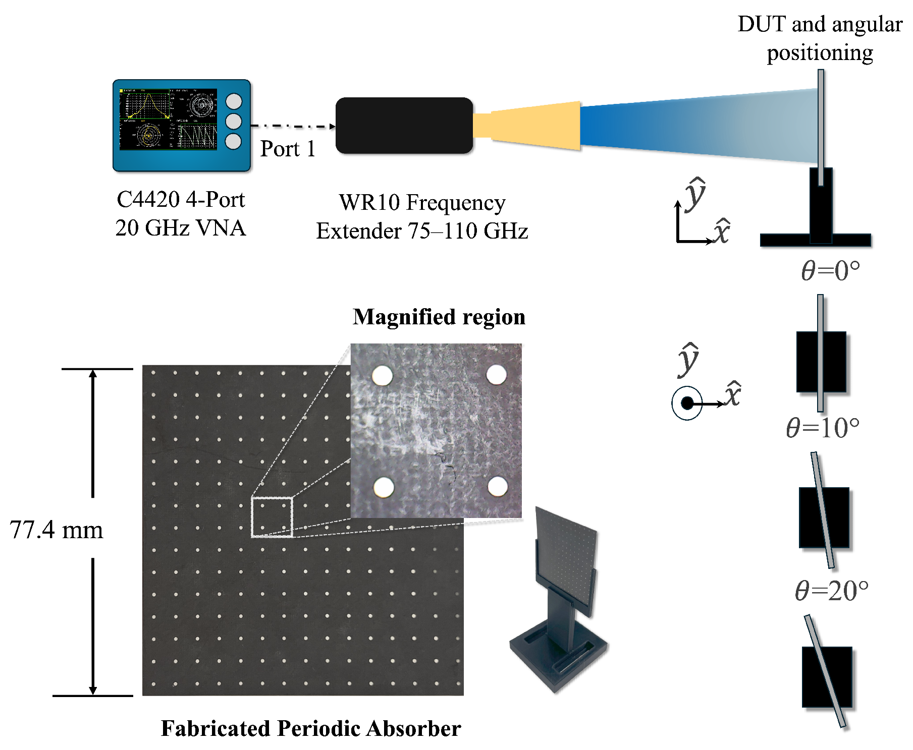
To validate the generated design experimentally, one CDCGAN-generated unit cell was fabricated on a Rogers 5880 substrate using standard PCB etching techniques. The prototype was fabricated on nominal $0.508$ mm RT/duroid 5880 with $35\mathsf{\mu }$m copper. Rogers specifies $D_k=2.20\pm 0.02$ and $tan\delta =0.0009$ at 10 GHz. The periodic array spans up to 15 unit cells, corresponding to approximately 18–$21{\lambda }_0$ across the 75–78 GHz band. This provides a sufficiently large periodic region for the illuminated area to approximate the response of the infinite periodic structure while limiting edge effects. The prototype was characterized in a free-space reflection measurement setup over the 75–78 GHz interval, as shown in Figure 7. To examine the angular behavior of the generated absorber used in the experimental validation (see Figure 8a), full-wave simulation and measurements were performed for different incidence angles $\theta$. For each angle, the reflected response of the absorber was measured together with an angle-matched metallic reference positioned at the same device-under-test (DUT) plane. The metallic-reference measurement was used to normalize the reflected response and thereby remove the frequency-dependent response of the measurement path. Defining the normalized complex reflection coefficient as ${\Gamma }_{\mathrm{norm}}(f,\theta )$, the experimental absorptance was calculated as

$$A_{\mathrm{meas}}(f,\theta )=1-{\left|{\Gamma }_{\mathrm{norm}}(f,\theta )\right|}^2.$$

(10)

Because the absorber contains a continuous metallic ground plane, transmission through the structure is neglected in the experimental power balance. Thus, the measured absorptance is obtained from the metallic-reference-normalized reflected power.

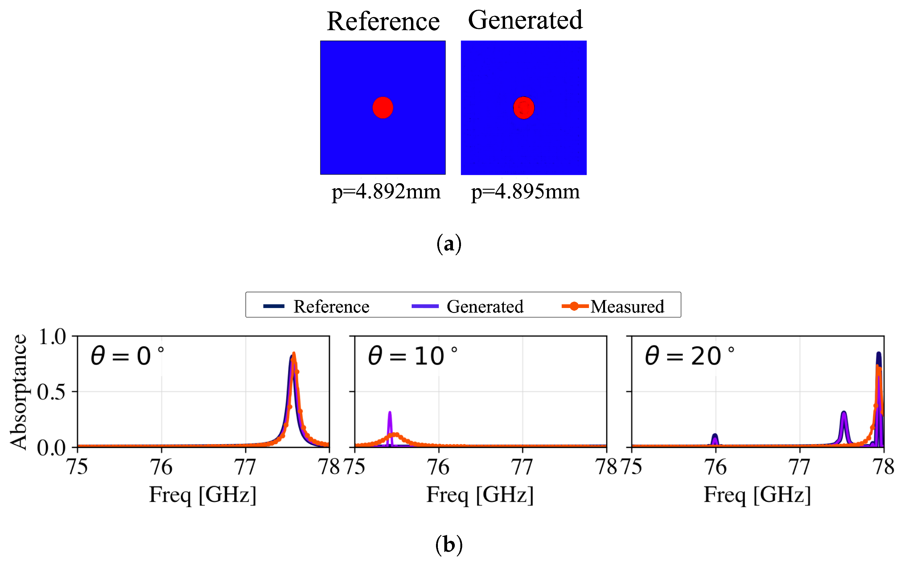
Figure 8 compares the reference HFSS response, the full-wave response of the reconstructed generated geometry, and the measured absorptance of the fabricated sample. The numerical values reported in

Table 3. Full-wave reconstruction accuracy of the CDCGAN-generated samples. The reported MSE values correspond to ${\mathrm{MSE}}_{\mathrm{ref}-\mathrm{gen}}$.

Figure	Shape	SSIM	CS $0^{\circ }$	${\mathbf{MSE}}_{\mathbf{ref}-\mathbf{gen}}$$0^{\circ }$	${\mathbf{MSE}}_{\mathbf{ref}-\mathbf{gen}}$${10}^{\circ }$	${\mathbf{MSE}}_{\mathbf{ref}-\mathbf{gen}}$${20}^{\circ }$	${\mathbf{MSE}}_{\mathbf{ref}-\mathbf{gen}}$${30}^{\circ }$
Figure 8	Circle	0.966	0.999	$1.48\times {10}^{-4}$	$9.37\times {10}^{-4}$	$2.16\times {10}^{-4}$	$1.77\times {10}^{-3}$
Figure 9a	Circle	0.974	0.990	$1.30\times {10}^{-2}$	$1.16\times {10}^{-4}$	$1.44\times {10}^{-2}$	$1.54\times {10}^{-3}$
Figure 9b	Circle	0.976	0.980	$1.63\times {10}^{-2}$	$4.78\times {10}^{-5}$	$4.66\times {10}^{-3}$	$1.74\times {10}^{-2}$
Figure 9c	Cross	0.965	0.917	$2.55\times {10}^{-2}$	$9.48\times {10}^{-3}$	$3.62\times {10}^{-3}$	$1.33\times {10}^{-3}$
Figure 9d	Cross	0.904	0.640	$3.18\times {10}^{-2}$	$6.72\times {10}^{-3}$	$2.51\times {10}^{-2}$	$2.11\times {10}^{-3}$
Figure 9e	Ring	0.967	0.950	$2.11\times {10}^{-3}$	$5.04\times {10}^{-4}$	$4.08\times {10}^{-2}$	$6.03\times {10}^{-3}$
Figure 9f	Ring	0.967	0.980	$2.74\times {10}^{-4}$	$1.34\times {10}^{-4}$	$2.01\times {10}^{-3}$	$1.39\times {10}^{-3}$

correspond to ${\mathrm{MSE}}_{\mathrm{ref}-\mathrm{gen}}$ and therefore quantify the reconstruction accuracy between the reference and generated HFSS models. A separate comparison is used to quantify the agreement between the fabricated sample and the generated-geometry simulation. The resulting ${\mathrm{MSE}}_{\mathrm{meas}-\mathrm{gen}}$ values are $7.60\times {10}^{-4}$, $1.17\times {10}^{-3}$, and $7.89\times {10}^{-3}$ at $\theta =0^{\circ }$, ${10}^{\circ }$, and ${20}^{\circ }$, respectively. At ${20}^{\circ }$, the dominant absorption feature remains centered near 77.9 GHz: the measured- and generated-HFSS peak frequencies are approximately 77.92 GHz and 77.94 GHz, respectively. The corresponding peak absorptances are approximately 0.736 and 0.697. At oblique incidence, small angular-positioning errors can introduce diffractive effects and modify the measured spectral response. The positioning uncertainty of our free-space setup is approximately $\pm 2^{\circ }$, which may contribute to the differences observed at ${20}^{\circ }$. Another possible source of discrepancy is the slight bending of the $0.508$ mm-thick substrate during mounting. Since the sample could not be maintained perfectly flat, small local variations in incidence angle and phase may occur across the illuminated area and affect the measured response.

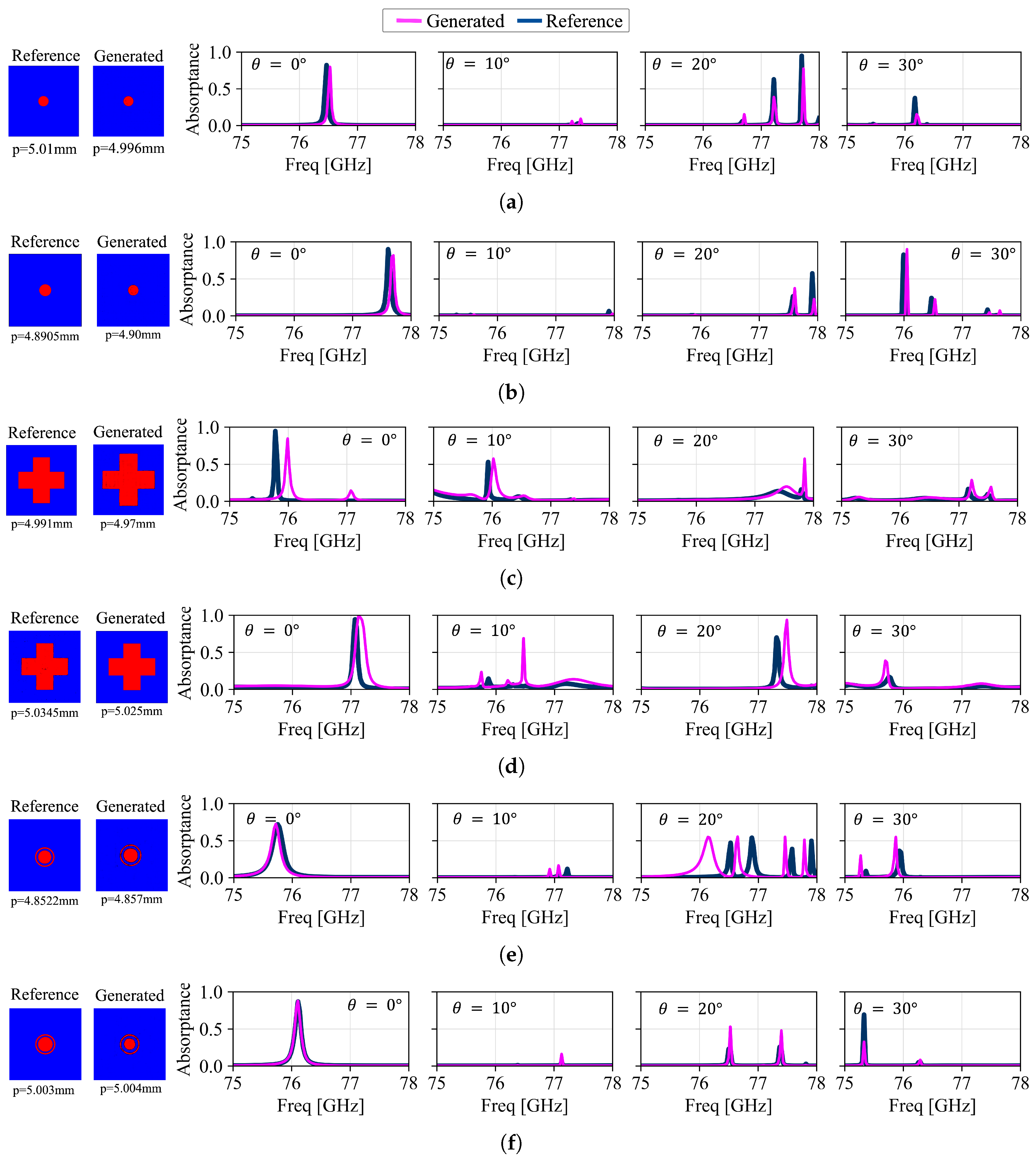
Figure 9 shows several representative CDCGAN-generated absorbers and compares their full-wave spectra with the corresponding reference structures. The reconstruction agreement is quantified by the SSIM, cosine similarity, and ${\mathrm{MSE}}_{\mathrm{ref}-\mathrm{gen}}$ values reported in Table 3. Some generated structures preserve the reference spectral response closely over the evaluated angular range, whereas others exhibit larger discrepancies at particular incidence angles. Notably, the model was trained exclusively using absorptance spectra corresponding to $\theta =0^{\circ }$. The responses shown at nonzero incidence angles therefore correspond to post-generation full-wave evaluations of the reconstructed unit cells rather than to angle-conditioned network predictions. The discrepancies observed in Figure 9 at ${20}^{\circ }$ and ${30}^{\circ }$ are not monotonic with incidence angle and vary from one generated geometry to another. For example, Figure 9b exhibits a larger error at ${30}^{\circ }$, whereas Figure 9d,e show their largest discrepancies at ${20}^{\circ }$ and improvement again at ${30}^{\circ }$. Conversely, Figure 9f maintains low ${\mathrm{MSE}}_{\mathrm{ref}-\mathrm{gen}}$ values at both angles. This behavior can be associated with the fact that the generated unit cells are not exact replicas of the reference structures. The decoded lattice period exhibits a small but finite reconstruction error, while the generated metallic contours also show small local differences with respect to the reference geometry. Small differences in the period or contour dimensions can become more electromagnetically significant at particular incidence angles. The case in Figure 9f illustrates this point particularly well. A close inspection of the reference and generated unit cells reveals small differences in the reconstructed ring dimensions and contour shape, yet the spectral agreement remains strong, with ${\mathrm{MSE}}_{\mathrm{ref}-\mathrm{gen}}=2.01\times {10}^{-3}$ at ${20}^{\circ }$ and $1.39\times {10}^{-3}$ at ${30}^{\circ }$. In other samples, comparable geometrical differences produce larger spectral deviations. Therefore, the angular discrepancies are interpreted as the combined electromagnetic consequence of small period- and topology-reconstruction errors rather than as a systematic loss of performance with increasing incidence angle. The CS metric, reaching up to 0.999, indicates that the generated curves closely match references, demonstrating the algorithm’s ability to accurately capture spectral features, i.e., absorptance profile height and bandwidth. This is also supported by the results obtained for the measured absorber.

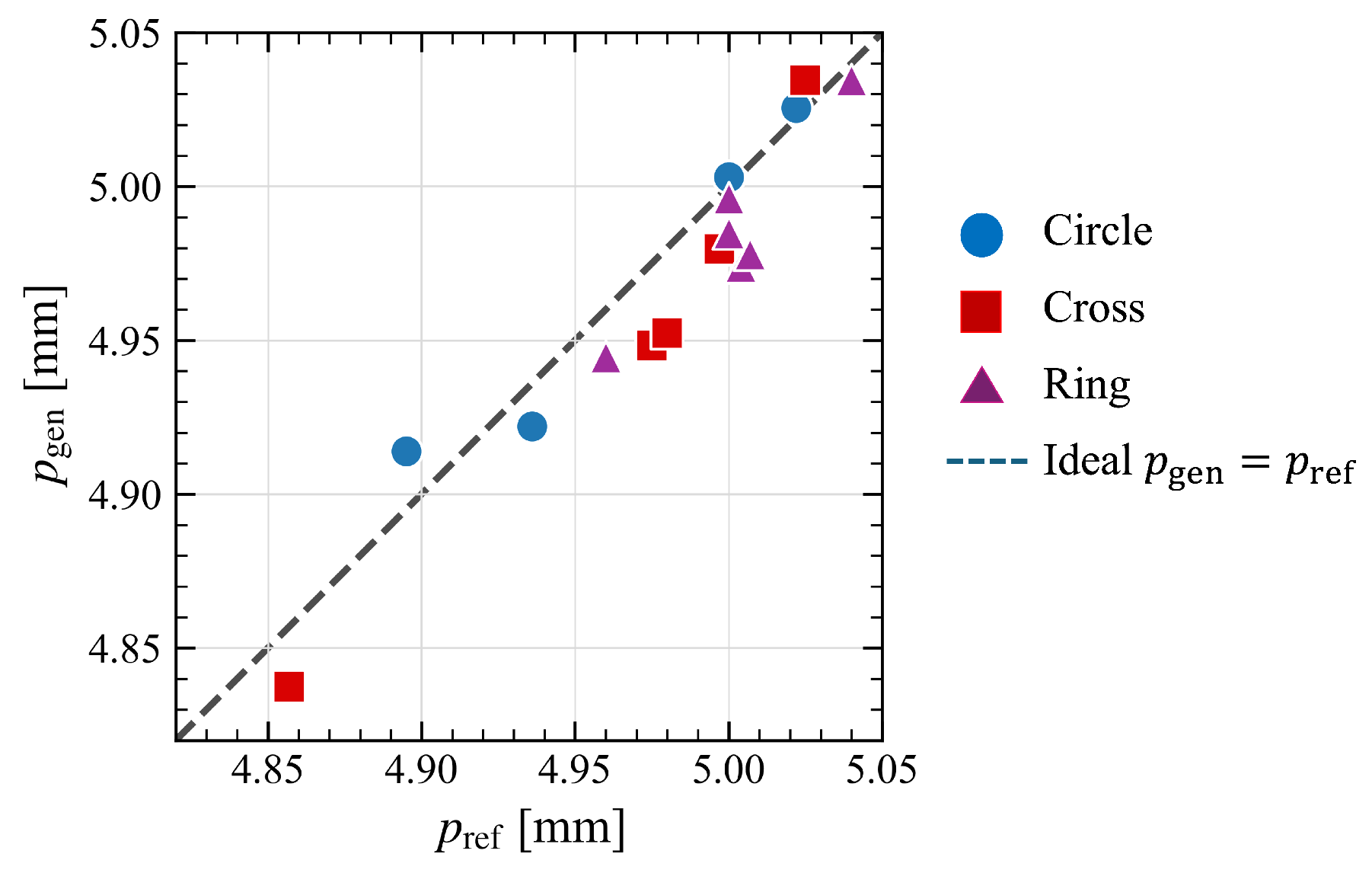
As for the varying-period feature, the lattice period constitutes an additional design degree of freedom that enables fine adjustment of the resonant response within the target frequency band. Figure 10 compares the reference period with the period decoded from the generated image for 15 representative samples. The mean absolute period error is defined as

$${\mathrm{MAE}}_p={\displaystyle \frac{1}{N}}{\displaystyle \sum _{i=1}^N}\left|p_{\mathrm{gen},i}-p_{\mathrm{ref},i}\right|,$$

(11)

where N is the number of evaluated unit cells, and $p_{\mathrm{gen}}$ and $p_{\mathrm{ref}}$ correspond to the decoded period from the generated image and the reference period, respectively. For the $N=15$ samples, the resulting ${\mathrm{MAE}}_p$ is $0.0159$ mm. The recovered periods closely follow the ideal $p_{\mathrm{gen}}=p_{\mathrm{ref}}$ relation, with a mean absolute error of $0.0159$ mm. These results validate the effectiveness of the lattice size fringe-encoding strategy for recovering unit-cell dimensions. This is demonstrated with the measured absorber, and further validation comes from simulations with varying incidence angles. The generated unit cells closely match the intended designs and exhibit behavior consistent with the originals. Finally, despite the low MSE, high CS, and strong SSIM, minor variability persists in cross-shaped unit cells, which is related to the growing complexity of the shapes. Spectral discrepancies arise from structural complexity, with slight arm dimension variations or differences in unit-cell period. Given that these results are obtained for variable-period, wavelength-scale unit cells and without any post-optimization loops, they show that a properly conditioned CDCGAN can already deliver high-fidelity, fabrication-ready absorber designs with a good angular response.

Comparative Analysis

To contextualize the proposed framework, we compare it against other AI-driven MS design methods (e.g., variational autoencoders (VAE) and deep neural network (DNN)) using qualitative and quantitative parameters. To contextualize how previous studies assess the quality of their reported results, it is useful to note that the adopted evaluation criteria vary considerably across the literature. Some works rely primarily on qualitative agreement between target and predicted spectra, whereas others report quantitative error metrics under their own specific prediction or inverse-design protocols. For example, Yeung et al. [38] reported MSE values on the order of $2\times {10}^{-3}$, Tezsezen et al. [39] reported approximately $8\times {10}^{-3}$, and Wang et al. [40] reported approximately $5\times {10}^{-3}$. Ma et al. [27] relied mainly on qualitative spectral agreement, while An et al. [21] reported errors on the order of ${10}^{-4}$ for their predictive network. These approaches differ not only in their electromagnetic objectives, but also in how the physical design itself is represented. The novelty of the present work therefore does not arise from the CDCGAN architecture alone. Rather, the principal distinction lies in the representation adopted for the inverse-design problem.

Our propose method supports multiple design degrees of freedom, as geometric and spectral parameters are encoded directly into the training images. In our implementation, we condition the generation process using a shape class vector, allowing the model to selectively produce cross-, ring-, or circle-shaped unit cells. This conditioning is flexible: additional parameters such as substrate type, layer count, or even polarization mode can be included in the conditioning vector during training. In comparison (

Table 4. Feature-based comparison of the proposed CDCGAN with representative AI-driven metasurface design approaches.

Feature	This Work	Ref. [16]	Ref. [21]	Ref. [41]
Design task	Inverse design of high-absorptance W-band metasurfaces	Inverse design of multilayer metasurfaces	Forward/inverse design of all-dielectric metasurfaces	Design of pixelated broadband absorbers (C- and X-band)
Design representation	$512\times 512$ RGB image with topology and lattice scale jointly represented	$52\times 52$ image-based multilayer representation	Geometric parameter vector	Binary pixelated unit-cell representation
Period variability	Variable within the trained $4.85$–$5.30$ mm domain; period encoded and recovered from the image fringe	Fixed in the reported formulation	Fixed in the reported formulation	Fixed-period unit cell
Input/conditioning	Target absorptance spectrum + spectral descriptors + shape class + latent vector	Flattened spatial representation combined with latent-space generation	Target response or geometric parameters, depending on forward/ inverse network	Reflection spectrum + Gaussian latent noise for CDCGAN generation
Training data	20,543 samples; circle, cross, and ring classes	$>30,000$ samples	14,800 “H” models and 50,000 cylindrical models	$>2000$ samples
Post-generation optimization	No separate iterative geometry-optimization stage; generated image is decoded, converted to CAD, and verified by full-wave simulation	Additional predictive/ design workflow used in the reported framework	Inverse-design stage operates together with the trained forward model	Additional prediction/ design stages are used in the reported workflow
Experimental validation	One fabricated generated absorber characterized in free space	Numerical validation	Numerical validation	Fabricated absorber with experimental verification
Angular evaluation	HFSS at $0^{\circ }$, ${10}^{\circ }$, ${20}^{\circ }$, and ${30}^{\circ }$; measurements at $0^{\circ }$, ${10}^{\circ }$, and ${20}^{\circ }$	Not used as a comparison criterion	Not used as a comparison criterion	Experimental validation reported at normal incidence

), Naseri and Hum [16] utilized a VAE to design multilayer MSs, with high degrees of freedom. Now, this model does not provide an explicit way to add conditioning to the generative process. The sampling method of the latent space is different as well, as we have noise and an added extra conditioning vector that supports and guides the sampling process. While the VAE approach is well-suited for exploring latent design spaces, it does not support conditional generation.

On the other hand, An et al. [21] introduced a DNN for phase and amplitude prediction in all-dielectric MSs. The DNN supports the use of input vector encoding the geometric information and training is performed over the specific shape of the unit cell, thus solving the forward problem of predicting the EM response from the geometric design. The inverse problem is tackled by using a network that receives the ideal spectra and produces a vector with the specific parameters for the geometry under study, namely, a cylinder. This is a simpler version as it does not use images to train the model. Although the model achieves high prediction accuracy, the model is limited to parameter-based representations of a single-shaped unit cell. As for the inverse design network, they rely on a meta-filter intended to produce the approximate geometrical parameters. Now, they do not provide the actual error by comparing the target spectral responses and the generated ones. By inspection, they look close but not necessarily fitted, as seen in Figure 6 of the aforementioned reference. Also, they only demonstrate the result based on simulations while not adding more results like changing incidence angles or fabricated measurements.

Further cases can be analyzed, but it is worth considering the following. He et al. [41] design pixelated C- and X-band absorbers using a transfer-learning network combined with a CDCGAN that outputs binary pixel maps on fixed-period unit cells (Table 4). The lattice period is neither encoded nor recovered, and there is no explicit near-unity absorptance target. Moreover, their experimental validation is reported only for normal incidence, and the agreement between simulation and measurement is discussed qualitatively, with discrepancies attributed to parameter error and the experimental environment. Hodge et al. [42] use DCGANs to generate reflective unit cells. Their GAN operates on $64\times 64$ unit-cell images with a fixed lattice and is conditioned only on the target reflection spectra, without the explicit encoding of additional spectral descriptors (such as peak positions or bandwidth) or meta-atom class, and the unit-cell period is not treated as a design variable. While they report good agreement for the reflective response in their RF setting, the approach does not address high-absorptance behavior, variable-period design, or high-resolution images. Mall et al. [43] propose a multi-model cyclic framework with several networks (forward predictor and inverse generator) combined with a genetic algorithm for optical MSs, operating on fixed unit-cell sizes and requiring explicit re-optimization. They report a best simulated case and cosine similarity for their objective, but the performance is evaluated at a single incidence condition, without studying how the generated designs behave under angle variation or including incidence angle in the conditioning.

It is important to highlight several practical differences in the design workflow. Although the training-set sizes are of a similar order, the present framework operates on higher-resolution $512\times 512$ images, which reduces the pixelation of the generated contours and can limit discretization artifacts during subsequent full-wave reconstruction. In addition to the target absorptance spectrum, the conditioning includes auxiliary descriptors such as shape class, peak information, and FWHM. Finally, while some reported inverse-design frameworks employ forward predictive models or additional optimization stages to refine the generated solution, the present approach directly decodes the generated topology and period and proceeds to full-wave verification without a separate post-generation optimization loop.

4. Conclusions

A CDCGAN model is presented that generates unit cells with high absorptance in the W-band with high structural and spectral fidelity while supporting variable period sizes. MSE and CS metrics confirm strong agreement between generated and reference absorptances. The simulated and measured results exhibit good response across various incidence angles, despite not counting them as training parameters. By embedding the unit-cell period in the blue channel fringe of the generated image, our model enables the precise tuning of spectral responses across a band without requiring model retraining or external optimization. This feature, uncommon in prior works where the lattice period is typically fixed, provides additional design flexibility within the period range represented by the training data. Extension to other frequency bands or broader operating ranges would require corresponding training data and, when necessary, the retraining or fine-tuning of the model. The comparative analysis highlights differences in representation and workflow among recent AI-driven metasurface design methods. In the present framework, the principal distinction is the joint representation of high-resolution unit-cell topology and lattice period, which improves design flexibility and facilitates extending the framework to other frequency bands, where the lattice period plays a key role in tuning the absorber response.

The framework supports the generation of diverse unit-cell geometries (circle, cross, ring), providing adaptability for various absorber applications. In scenarios where the unit-cell size is closer to the wavelength, our approach ensures high geometric precision through high-resolution images, minimizing pixelation artifacts and maintaining well-defined shapes to achieve accurate electromagnetic responses. Further refinement is needed to improve the geometric precision of patches and their periods, which can be achieved through interpolation strategies or optimization algorithms. However, as geometry complexity or shape variety increases, training becomes more challenging. To address this, ongoing efforts integrate Transformers or ResNet-based architectures to refine outcomes. These techniques aim to enhance the precision and adaptability of generated unit cells, bridging the gap between AI-driven design and practical MS implementation.