Machine Learning Based on Hybrid Optimization Algorithm for the Prediction and Risk Assessment of Rock Tunnel Lining Displacement

Abstract

Accurate prediction of tunnel vault displacement and reliable assessment of deformation risk are essential for tunnel safety management under complex geological conditions. This study develops an integrated data-driven framework combining machine-learning prediction, metaheuristic hyperparameter optimization, statistical model comparison, and uncertainty-informed relative deformation-severity classification. Four baseline models, namely BP, SVM, LSTM, and Peephole-LSTM, were combined with GA, WOA, and PSO to construct 12 optimized models, resulting in 16 candidate models. Monitoring observations were chronologically divided into training, validation, and test sets at a ratio of 70%:15%:15%, and normalization parameters were calculated exclusively from the training set to prevent data leakage. Model robustness was further evaluated using rolling validation, the Friedman test, and post hoc Wilcoxon signed-rank tests with Holm correction. PSO-Peephole-LSTM achieved the best test-set performance, with an MAE of 0.058 mm, an RMSE of 0.074 mm, and an R² of 0.884. PSO-Peephole-LSTM also achieved the lowest mean RMSE and average rank across the rolling validation windows, with statistically significant improvements over the competing models after Holm correction. Finally, 2000 Latin hypercube samples were generated to propagate prediction uncertainty and establish a five-level, project-specific relative deformation-severity classification framework. The integrated workflow provides a systematic connection between tunnel monitoring, displacement forecasting, uncertainty characterization, and uncertainty-informed monitoring and decision support.

1. Introduction

Tunnel deformation reflects the response of the tunnel system to stress redistribution, geological conditions, and environmental disturbances, and is therefore widely regarded as a key indicator of structural performance and operational safety [1,2,3]. In newly constructed tunnels, deformation continues to develop during construction and the early stages of operation as the surrounding rock mass gradually reaches a new equilibrium state. Continuous observation and reliable prediction of deformation are consequently required for stability assessment, hazard identification, and maintenance planning.

The development of monitoring technologies has provided unprecedented opportunities for understanding tunnel behaviour. Three-dimensional laser scanning [4,5], Wireless Sensor Networks (WSNs) [6], and other sensing technologies enable continuous acquisition of temperature, stress, strain, and displacement data [7,8]. Through real-time transmission and long-term storage of monitoring information, WSN-based systems have become an important component of modern tunnel monitoring frameworks [9,10,11,12]. The increasing availability of monitoring data has shifted attention from data acquisition to data interpretation, creating a demand for methods capable of extracting meaningful information from complex monitoring records.

Machine learning (ML) has emerged as an effective tool for addressing this challenge because of its ability to establish nonlinear relationships directly from data [13,14]. Early applications in tunnel engineering mainly relied on Back Propagation (BP) neural networks [15] and Support Vector Machines (SVM) [16] to predict tunnel responses from monitoring variables. With the accumulation of long-term monitoring data, attention has gradually expanded towards deep learning approaches, particularly Long Short-Term Memory (LSTM) networks and Gated Recurrent Units (GRU), which are well suited to modelling temporal dependencies in sequential data [17,18,19,20]. These developments have extended the capability of data-driven methods for tunnel deformation prediction. More recently, Transformer-based models have been introduced into tunnelling time-series forecasting to capture long-range dependencies within multivariate monitoring data [21]. Meanwhile, Bayesian and uncertainty-aware neural networks have been applied to structural safety assessment to quantify predictive uncertainty beyond deterministic point estimates [22]. Explainable tunnel deformation models have also used SHAP to identify influential temporal and static factors, thereby improving the transparency of data-driven predictions [23]. These developments broaden the methodological landscape of structural health monitoring, although their data and computational requirements may restrict their application to relatively small tunnel-monitoring datasets.

Nevertheless, the prediction performance reported in the literature varies considerably across different studies. One reason is that the effectiveness of machine learning models depends strongly on hyperparameter selection. Model calibration influences the representation of complex deformation patterns and directly affects prediction accuracy and generalization capability. To improve model performance, metaheuristic optimization algorithms have been coupled with machine learning models in a variety of engineering applications. However, existing tunnel studies generally focus on individual model configurations, making it difficult to assess the relative merits of different optimization strategies and their interactions with different prediction models.

A further limitation lies in the manner in which prediction results are interpreted. Most existing studies focus on deterministic prediction and evaluate model performance using statistical error metrics. While such measures are useful for assessing predictive accuracy, they provide limited information regarding the uncertainty associated with future tunnel behaviour. Tunnel deformation is influenced by geological variability, environmental fluctuations, measurement errors, and model uncertainty, all of which contribute to uncertainty in future responses. Consequently, a deterministic displacement estimate alone does not directly indicate the level of operational risk. For practical tunnel management, prediction results need to be linked to uncertainty-informed and project-specific indicators of relative deformation severity so that monitoring information can be translated into actionable risk indicators.

To address these gaps, this study develops an integrated data-driven framework that extends deterministic tunnel deformation prediction to uncertainty-informed relative deformation-severity assessment. In contrast to recent studies such as DCSGN, which primarily focus on deformation prediction, the proposed framework connects model optimization and validation with uncertainty propagation and risk classification. A highway tunnel in Shandong Province, China, is adopted as a case study. Four baseline models, namely back-propagation neural network (BP), support vector machine (SVM), long short-term memory network (LSTM), and Peephole-LSTM, are combined with genetic algorithm (GA), whale optimization algorithm (WOA), and particle swarm optimization (PSO), resulting in 16 candidate models. The models are developed and evaluated using a chronological training–validation–test split, training-set-based normalization, rolling time-series validation, and nonparametric statistical comparisons. The optimal model is subsequently integrated with Latin hypercube sampling to propagate prediction uncertainty and classify tunnel vault displacement into five project-specific relative deformation-severity levels. The framework-level contribution of this study is therefore a unified prediction–validation–uncertainty–risk classification workflow that translates deterministic displacement forecasts into uncertainty-informed relative deformation-severity information for tunnel monitoring and decision support.

2. Methodology

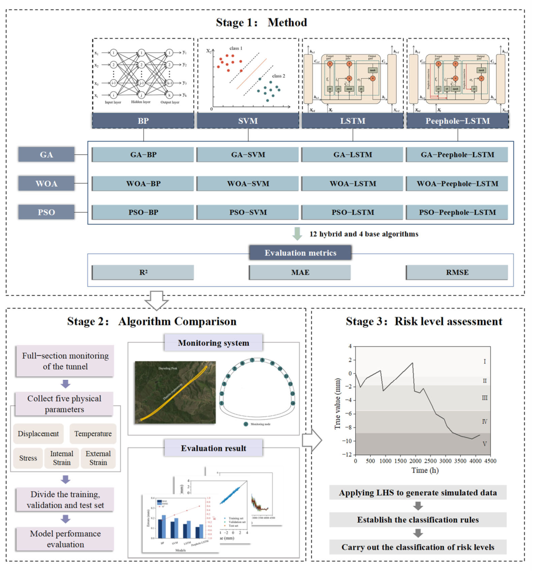
Figure 1 illustrates the framework developed for tunnel vault displacement prediction and probabilistic risk assessment. The framework consists of model development, performance evaluation, and risk assessment. Four machine learning models, namely BP, SVM, LSTM, and Peephole-LSTM, were combined with three optimization algorithms, including GA, WOA, and PSO, to construct twelve hybrid prediction models. Together with the four baseline models, a total of sixteen prediction models were established and evaluated. The prediction models were trained and validated using monitoring data collected from the tunnel, including displacement, temperature, stress, internal strain, and external strain measurements. Model performance was assessed using the coefficient of determination (R²), mean absolute error (MAE), and root mean square error (RMSE). Based on the comparative analysis of the prediction results, the hyperparameter configuration of each model was selected according to its validation-set RMSE, and final predictive performance was evaluated using the independent test set. Subsequently, the selected optimal model was employed to predict tunnel vault displacement. To account for the uncertainty associated with the prediction results, Latin Hypercube Sampling (LHS) was incorporated to characterize the probabilistic distribution of tunnel deformation. The predicted displacement responses were then classified into different risk levels according to project-specific displacement intervals, enabling temporal characterization of relative deformation severity. The integrated framework combines deformation prediction and risk assessment, providing a basis for risk-informed tunnel monitoring and management.

2.1. Machine Learning Method

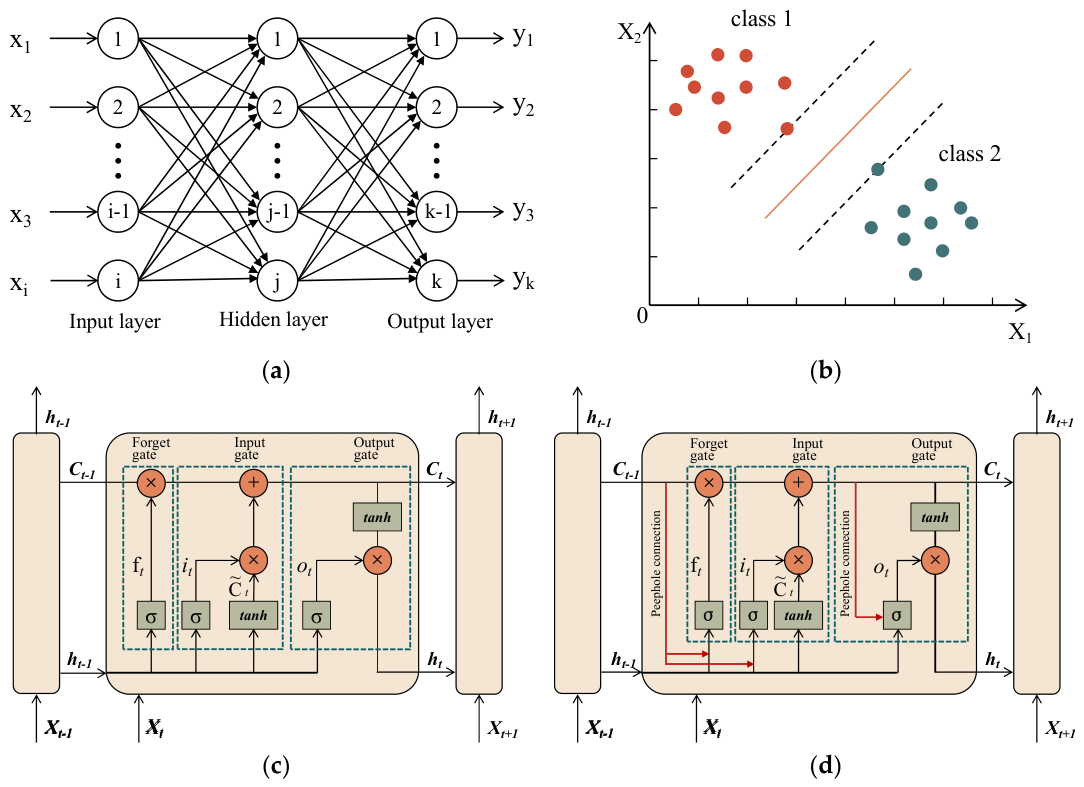
Figure 2 illustrates the architectures of the four machine learning models adopted in this study. These models represent different learning paradigms and provide a comprehensive basis for evaluating tunnel displacement prediction performance. The BP neural network, shown in Figure 2a, is a multilayer feedforward network consisting of an input layer, one or more hidden layers, and an output layer. Model parameters are updated through error backpropagation to minimize the prediction error during training. Owing to its relatively simple architecture and nonlinear mapping capability, BP has been widely applied to engineering prediction problems. Figure 2b presents the structure of the Support Vector Machine (SVM), a supervised learning algorithm based on statistical learning theory. SVM establishes an optimal decision function by maximizing the margin between support vectors and the separating hyperplane. Through the kernel mapping mechanism, SVM can effectively capture nonlinear relationships and has demonstrated strong generalization capability when dealing with limited and high-dimensional datasets [24].

The LSTM network shown in Figure 2c is a recurrent neural network specifically developed for sequential data modelling [25]. The network incorporates a memory cell together with forget, input, and output gates, enabling the selective retention, updating, and transmission of information. This gating mechanism alleviates the gradient vanishing problem encountered in conventional recurrent neural networks and allows the model to capture long-term temporal dependencies in monitoring data. The operations of the forget gate, input gate, cell state update, output gate, and hidden state are described by Equations (1)–(5), respectively.

$$f_t=\sigma \left(W_f\times \left[h_{t-1},x_t\right]+b_f\right)$$

(1)

$$i_t=\sigma \left(W_i\times \left[h_{t-1},x_t\right]+b_i\right)$$

(2)

$$C_t=f_t\otimes C_{t-1}+i_t\otimes \left(\tanh \left(W_c\times \left[h_{t-1},x_t\right]+b_c\right)\right)$$

(3)

$$o_t=\sigma \left(W_o\times \left[h_{t-1},x_t\right]+b_o\right)$$

(4)

$$h_t=O_t\times \tanh \left(C_t\right)$$

(5)

where h_t−1 is the hidden state from the previous cell, x_t is the input at the current moment, c_t is the output state of the current cell, W and b are the weight and bias, respectively, and $\otimes$ is the multiply of elements in corresponding vectors.

The Peephole-LSTM architecture incorporates additional connections between the cell state and the gating units [26], as shown in Figure 2d. By allowing the forget, input, and output gates to access the cell state directly, the gating process is informed by both the hidden state and the internal memory state. This modification enriches the information available for gate activation and improves the representation of long-term temporal dependencies in sequential data.

2.2. Optimization Algorithm

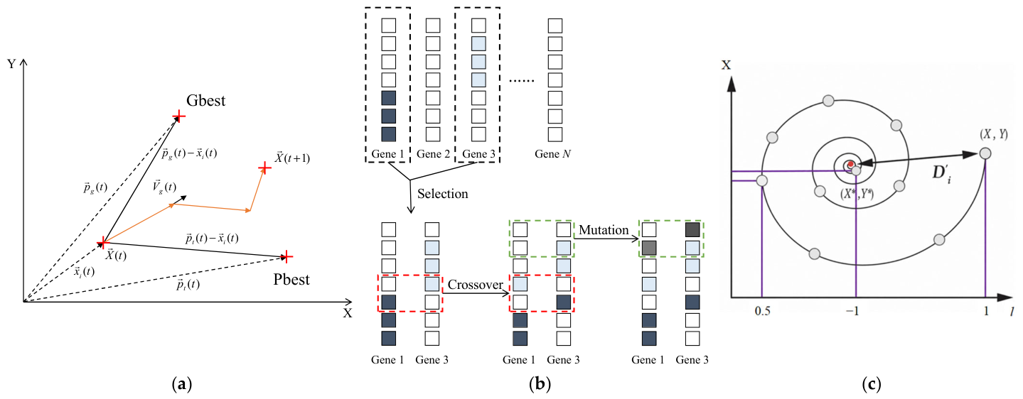
Particle Swarm Optimization (PSO), Genetic Algorithm (GA), and Whale Optimization Algorithm (WOA) were employed to optimize the hyperparameters of the machine-learning models. The corresponding optimization procedures are illustrated in Figure 3a–c. As shown in Figure 3a, PSO updates the velocity and position of each particle according to its individual best solution (Pbest) and the global best solution (Gbest), enabling the particle swarm to progressively approach promising regions of the search space [27]. Figure 3b illustrates the evolutionary process of GA, in which candidate solutions are updated through selection, crossover, and mutation operations. The fitness of each individual is evaluated in every generation, and better-performing solutions are retained for subsequent evolution [28,29]. As shown in Figure 3c, WOA is inspired by the bubble-net hunting behaviour of humpback whales. It searches for optimal solutions through mechanisms including prey encircling, spiral bubble-net attacking, and random exploration, thereby balancing global exploration and local exploitation [30]. In this study, PSO, GA, and WOA were separately coupled with BP, SVM, LSTM, and Peephole-LSTM to determine optimal hyperparameter combinations and evaluate the influence of different optimization strategies on tunnel displacement prediction.

3. Case Study

3.1. Project Overview

The tunnel investigated in this study is located within a nature reserve in eastern China. Both the left and right bores exceed 3000 m in length, making it the second-longest tunnel in Shandong Province. During construction, the project encountered highly variable geological conditions, including frequent transitions in surrounding rock classification and sections with extremely shallow overburden, with a minimum burial depth of 3.7 m. These conditions resulted in pronounced spatial variability in tunnel response and posed significant challenges to construction safety.

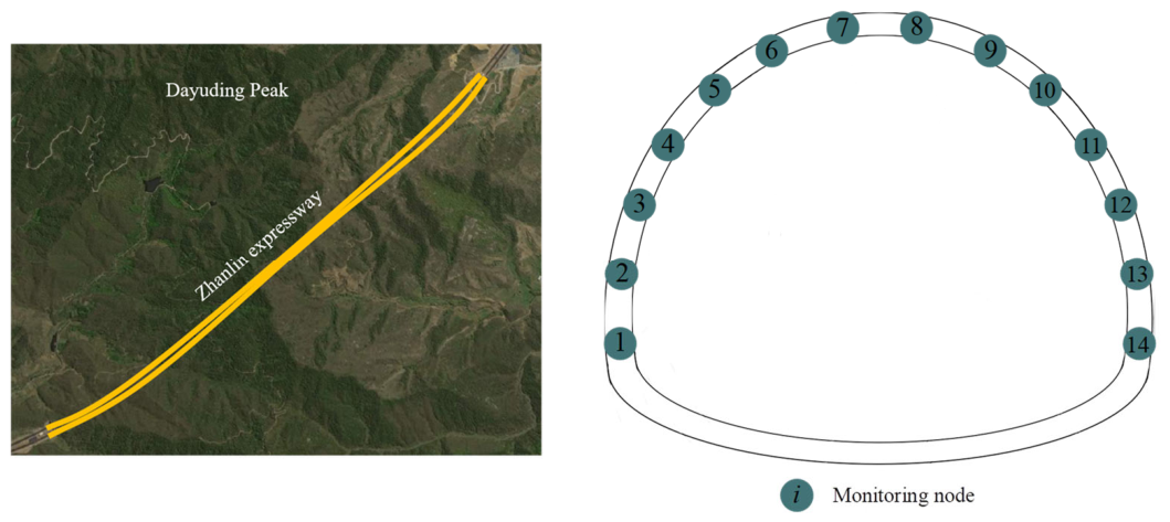
Particular attention was given to a fractured rock zone, where excavation-induced stress redistribution was expected to generate substantial deformation. To capture the deformation characteristics under these unfavorable geological conditions, a monitoring section was established at the center of the fractured rock zone [31]. The location of the tunnel and the monitoring section are shown in Figure 4.

Reliable deformation prediction depends on the acquisition of representative monitoring data. Previous studies have identified temperature, stress, and strain as key factors influencing tunnel deformation [11]. Accordingly, a monitoring system was established to continuously record four types of measurements, namely temperature, stress, strain, and structural displacement. These parameters were subsequently used as input variables for the machine learning models developed in this study.

Given the pronounced spatial variability of deformation in newly constructed tunnels, particularly in fractured rock environments, a dense sensor arrangement was adopted to capture the deformation behaviour across the entire tunnel cross-section. As illustrated in Figure 4, each monitoring location was equipped with an earth pressure cell, a temperature sensor, a displacement meter, and two strain gauges installed on the primary and secondary linings, respectively. The resulting monitoring data provided the basis for model training, validation, and subsequent risk assessment. The monitoring campaign was conducted from 16 January to 16 July 2024, yielding 4368 observations at an hourly sampling interval. Monitoring data were collected at an hourly sampling interval. A total of 14 monitoring nodes were arranged along the tunnel cross-section. At each node, four types of monitoring variables were recorded, including temperature, stress, strain, and structural displacement. These multisource monitoring records provided the data basis for subsequent tunnel vault displacement prediction and risk assessment.

3.2. Dataset Construction

The dataset was compiled from published monitoring records obtained at monitoring node 8, located at the tunnel vault. The monitored variables comprised vault displacement, temperature, stress, and strain in the primary and secondary linings. The records had undergone quality control and preliminary preprocessing in the original study. No missing observations were present in the dataset used herein; therefore, no additional data-cleaning procedures were applied. The monitoring campaign yielded 4368 hourly observations. Using a sliding window with a 6 h input sequence and a 1 h prediction horizon, these observations were transformed into 4362 supervised input–output samples.

The resulting samples were chronologically divided into training, validation, and testing subsets at a ratio of 70%:15%:15%, corresponding to 3053, 654, and 655 samples, respectively. The training set was used for model fitting, the validation set for hyperparameter optimization and model selection, and the independent testing set exclusively for the final unbiased evaluation. Descriptive statistics and missing-data information for the variables used in model development are provided in Table S1.

To prevent data leakage, the parameters required for min–max normalization were calculated exclusively from the training set and subsequently applied unchanged to the validation and testing sets. For each variable, the normalized value was calculated as follows:

$$x_s={\displaystyle \frac{x-x_{\min }}{x_{\max }-x_{\min }}}$$

(6)

where x_min and x_max denote the minimum and maximum values of the corresponding variable in the training set, respectively.

Following the temporal configuration adopted in the DCSGN study, supervised samples were constructed using a sliding-window strategy. Monitoring variables from the preceding 6 h were used as model inputs to predict the tunnel vault displacement at the subsequent 1 h time step. Accordingly, the input-window length and prediction horizon were set to 6 h and 1 h, respectively.

3.3. Model Development and Evaluation

Hyperparameters with a significant influence on model performance were selected for optimization. The optimized hyperparameters and their corresponding search ranges are summarized in

Table 1. Optimized hyperparameters.

Models	Hyperparameter	Search Range
SVM	C	[0.1, 1000]
	γ	[10−4, 10]
BP/LSTM/Peephole-LSTM	Batch size	{16, 32, 64, 128}
	Learning rate	[10−4, 10−2]
	Hidden layer dimension	{32, 48, 64, …, 256}

. To investigate the effectiveness of different optimization strategies, PSO, GA, and WOA were employed to determine the optimal hyperparameter combinations. Model performance was evaluated using the coefficient of determination (R²), root mean square error (RMSE), and mean absolute error (MAE). R², RMSE, and MAE were used to quantify predictive accuracy. The corresponding formulations of R², RMSE, and MAE are given in Equations (7)–(9).

To ensure a fair comparison, GA, PSO, and WOA were assigned an identical population size of 30 and a maximum of 100 iterations, corresponding to 3000 candidate-solution evaluations per run. All searches terminated after 100 iterations without early stopping. GA employed binary tournament selection, an elite size of 1, a crossover probability of 0.8, and a mutation probability of 0.1. For PSO, the inertia weight decreased linearly from 0.9 to 0.4, the cognitive and social learning factors were both set to 2.0, and the maximum particle velocity was limited to 20% of the corresponding parameter range. For WOA, the control parameter a decreased linearly from 2 to 0, the spiral-shape constant b was set to 1, and the spiral update probability was set to 0.5.

Each model–optimizer combination was independently executed ten times using random seeds from 2026 to 2035, with validation-set RMSE as the single optimization objective. For each run, the lowest validation RMSE and its associated hyperparameter configuration were recorded. The final configuration was selected as the one achieving the lowest validation RMSE across the ten runs, while the mean and standard deviation of the ten best validation RMSE values were used to characterize stochastic variability. Because this best-of-ten selection may yield an optimistic validation estimate, the validation score was used only for configuration selection and was not interpreted as an estimate of generalization performance. The selected configuration was subsequently fixed and evaluated on the independent test set, which remained excluded from run selection, hyperparameter optimization, and all other model-development decisions. The principal conclusions were therefore based on the independent test results and rolling-validation analysis. Representative learning-curve and residual diagnostics are provided in Figures S1 and S2 in the Supplementary Materials, respectively; these diagnostics are illustrative rather than exhaustive for all 16 models.

To evaluate the temporal robustness of the candidate models, an expanding-window time-series validation procedure was applied within the chronological training subset. The first 60% of the training data constituted the initial training interval. The remaining 40% was chronologically divided into ten consecutive and approximately equal validation blocks, each representing 4% of the training subset. For window Wk (k = 1, …, 10), the training interval comprised the first [60 + 4(k − 1)]% of the training data. The subsequent 4% constituted the corresponding validation interval. Thus, W1 used the first 60% for training and the following 4% for validation. W10 used the first 96% for training and the final 4% for validation. The training interval expanded by 4% between consecutive windows, while the validation intervals remained non-overlapping. All 16 models were evaluated using identical temporal partitions. For each window, the model parameters were reinitialized and retrained using only the observations available within the corresponding training interval. The previously selected hyperparameter configurations were held fixed and were not reoptimized for individual windows. The rolling-validation results were used exclusively to evaluate temporal robustness and conduct paired statistical comparisons, without affecting the independent final test-set evaluation.

To provide a simple temporal reference under the same experimental conditions, a persistence predictor was additionally evaluated. Given the 1 h prediction horizon, this baseline assumed that the displacement at the next time step was equal to the most recently observed displacement, such that ${\widehat{y}}_{t+1}=y_t$. The persistence predictor required neither model training nor hyperparameter optimization. It was evaluated using the same target timestamps, chronological data partition, rolling-validation intervals, and performance metrics as the 16 candidate models. All evaluation metrics were calculated on the original displacement scale in millimetres.

$$R^2=1-{\displaystyle \frac{{\displaystyle \sum _i^m{\left({\widehat{y}}_i-y_i\right)}^2}}{{\displaystyle \sum _i^m{\left(\overline{y}-y_i\right)}^2}}}$$

(7)

$$\mathrm{RMSE}=\sqrt{{\displaystyle \frac{1}{m}}{\displaystyle \sum _{i=1}^m{\left(y_i-{\widehat{y}}_i\right)}^2}}$$

(8)

$$\mathrm{MAE}={\displaystyle \frac{1}{m}}{\displaystyle \sum _{i=1}^m\left|y_i-{\widehat{y}}_i\right|}$$

(9)

where $y_i$ represents the true value of the sample; ${\widehat{y}}_i$ represents the corresponding predicted value; $\overline{y}$ is the average of the sample true values.

4. Results and Discussion

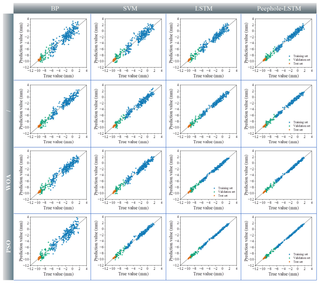
The predictive performance of the 16 models is illustrated in Figure 5, where the predicted tunnel vault displacements are compared with the corresponding measured values. Overall, the data points of the optimized models are more closely distributed around the reference line y = x than those of the corresponding baseline models, indicating improved prediction accuracy. The GA- and WOA-based models show varying degrees of improvement, whereas the PSO-based models exhibit the tightest clustering around the reference line. In particular, the PSO-LSTM and PSO-Peephole-LSTM models show the smallest dispersion across the training, validation, and test sets, demonstrating the strongest agreement between the predicted and measured displacements.

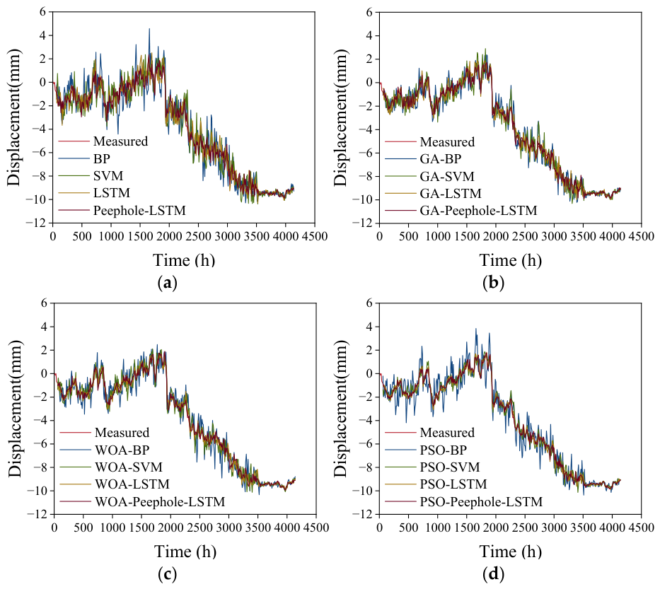
Figure 6 further compares the displacement time histories predicted by the 16 models with the monitoring data. Differences in predictive capability can be observed among the various model configurations. The basic machine learning models exhibit varying degrees of deviation from the measured values, whereas the optimized models generally provide improved prediction accuracy. In particular, the PSO-Peephole-LSTM and WOA-Peephole-LSTM models reproduce the overall deformation trend and local fluctuations more closely than the other models, demonstrating the effectiveness of PSO-based hyperparameter optimization for tunnel displacement prediction.

4.1. Performance Comparison of Prediction Models

Table 2. Ranking of model performance.

Rank	Models	Test Set
		MAE	RMSE	R2
1	PSO-Peephole-LSTM	0.058	0.074	0.884
2	WOA-Peephole-LSTM	0.07	0.088	0.835
3	PSO-LSTM	0.072	0.091	0.825
4	GA-Peephole-LSTM	0.092	0.116	0.720
5	WOA-LSTM	0.093	0.118	0.710
6	PSO-SVM	0.107	0.134	0.625
7	GA-LSTM	0.110	0.137	0.610
8	Peephole-LSTM	0.112	0.138	0.600
9	WOA-SVM	0.120	0.150	0.535
10	LSTM	0.141	0.173	0.380
11	GA-SVM	0.144	0.177	0.350
12	PSO-BP	0.147	0.181	0.320
13	WOA-BP	0.154	0.190	0.250
14	SVM	0.165	0.200	0.160
15	GA-BP	0.172	0.209	0.090
16	BP	0.187	0.230	−0.110
-	DCSGN	0.087	0.110	0.730
-	Persistence predictor	0.149	0.196	0.336

summarizes the testing-set performance of the 16 models developed and evaluated under the same experimental protocol. The performance values reported for DCSGN are also presented as a contextual reference but are excluded from the direct model ranking. The original DCSGN study did not fully report or publicly provide all the information required to reproduce its exact experimental conditions. Consequently, the models developed in the present study could not be configured, trained, and evaluated under the same conditions as DCSGN, precluding a rigorous direct comparison.

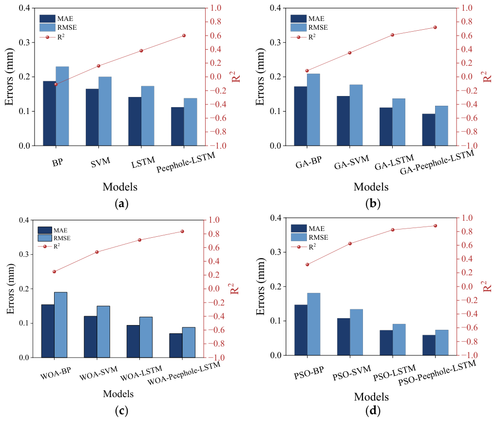
Considerable differences in predictive accuracy were observed among the 16 directly comparable models. PSO-Peephole-LSTM achieved the best overall performance, with the lowest MAE (0.058 mm) and RMSE (0.074 mm) and the highest R² (0.884), followed by WOA-Peephole-LSTM and PSO-LSTM. Moreover, the PSO-based variant achieved the best performance within each corresponding model family. These results demonstrate that the effectiveness of hyperparameter optimization depends on both the optimization algorithm and the underlying prediction architecture. In particular, combining PSO with recurrent neural networks improved the ability to capture the nonlinear and temporal characteristics of tunnel vault displacement. The DCSGN values reported in the original study, including an MAE of 0.087 mm, an RMSE of 0.110 mm, and an R² of 0.730, are provided solely to contextualize the present results within the existing literature and should not be interpreted as a direct benchmark comparison.

The persistence predictor achieved an MAE of 0.149 mm, an RMSE of 0.196 mm, and an R² of 0.336 on the independent test set. Relative to the persistence baseline, PSO-Peephole-LSTM reduced MAE and RMSE by 61.1% and 62.2%, respectively, while increasing R² by 0.548. These results demonstrate that the selected model provides substantial predictive improvement beyond simply carrying the most recent displacement observation forward by one hour.

Figure 7 presents the performance metrics of the evaluated models on the test set using a dual-axis representation. Noticeable differences can be observed among the various model configurations. In general, the incorporation of optimization algorithms improved the predictive performance of the corresponding base models, although the magnitude of improvement varied across model types. Among the three optimization strategies, PSO produced the largest improvement in prediction accuracy, particularly for the LSTM-based models. In contrast, the performance gains achieved by GA and WOA were comparatively limited. These results indicate that the effectiveness of hyperparameter optimization depends not only on the optimization algorithm itself but also on the underlying prediction model. With respect to the base models, the recurrent neural network architectures consistently outperformed BP and SVM. In particular, Peephole-LSTM achieved the highest prediction accuracy among the unoptimized models. The superior performance of the LSTM-based models can be attributed to their ability to capture temporal dependencies and nonlinear relationships in tunnel monitoring data, whereas the additional cell-state connections in Peephole-LSTM facilitate more effective information transfer during sequence learning.

Table 3. Optimal hyperparameters of the three selected recurrent models.

Model	Batch Size	Learning Rate	Hidden Layer Dimension
PSO-Peephole-LSTM	32	0.0013	128
WOA-Peephole-LSTM	64	0.0010	112
PSO-LSTM	32	0.0018	96

presents the optimal hyperparameter combinations of the three recurrent models selected for detailed analysis based on their validation performance. PSO-Peephole-LSTM selected a batch size of 32, a learning rate of 0.0013, and a hidden-layer dimension of 128. WOA-Peephole-LSTM adopted a larger batch size of 64, together with a learning rate of 0.0010 and a hidden-layer dimension of 112. For PSO-LSTM, the optimal configuration consisted of a batch size of 32, a learning rate of 0.0018, and a hidden-layer dimension of 96. All selected values fell within the predefined search ranges reported in Table 1. The differences among these configurations indicate that the optimal hyperparameter combination depends on both the prediction architecture and the associated optimization algorithm. After model selection using the validation data, these hyperparameters were fixed and applied unchanged during final testing. Although the resulting point estimates demonstrate the strong predictive performance of these models, further statistical analysis is required to determine whether the observed differences are statistically significant.

4.2. Statistical Significance Analysis of Model Performance

Statistical significance was evaluated using the RMSE values obtained by all 16 models over the same ten rolling-validation windows, which constituted paired observations within each temporal evaluation block.

Table 4. Rolling-validation RMSE and variability of the 16 prediction models.

Model	W1	W2	W3	W4	W5	W6	W7	W8	W9	W10	Mean RMSE	SD
BP	1.060	1.293	0.814	0.938	1.335	0.547	0.997	1.219	0.720	0.646	0.957	0.275
SVM	1.224	0.625	0.839	0.562	0.721	0.689	0.914	1.187	0.995	1.084	0.884	0.235
LSTM	0.937	0.633	0.383	0.928	0.689	0.570	0.772	0.872	1.008	0.688	0.748	0.193
Peephole-LSTM	0.805	0.657	0.866	0.811	0.455	0.595	0.900	0.377	0.685	0.740	0.689	0.173
GA-BP	0.585	0.797	1.262	0.896	0.913	1.029	0.518	1.221	1.117	0.712	0.905	0.256
GA-SVM	0.909	1.007	1.049	0.848	0.347	0.755	0.556	0.657	0.690	0.892	0.771	0.216
GA-LSTM	0.581	0.702	0.358	0.680	0.682	0.772	0.794	0.592	0.486	0.862	0.651	0.151
GA-Peephole-LSTM	0.668	0.638	0.584	0.506	0.604	0.505	0.531	0.595	0.663	0.386	0.568	0.087
WOA-BP	0.718	0.909	0.810	0.996	0.630	1.177	1.017	0.619	1.098	0.385	0.836	0.249
WOA-SVM	0.950	0.625	0.492	0.793	0.304	0.822	0.900	0.890	0.652	0.723	0.715	0.202
WOA-LSTM	0.449	0.744	0.494	0.676	0.546	0.370	0.599	0.726	0.559	0.685	0.585	0.124
WOA-Peephole-LSTM	0.444	0.500	0.541	0.539	0.489	0.572	0.481	0.483	0.514	0.367	0.493	0.057
PSO-BP	0.626	0.883	0.784	0.756	1.039	0.945	1.132	0.402	0.583	1.021	0.817	0.231
PSO-SVM	0.711	0.503	0.330	0.699	0.735	0.528	0.579	0.652	0.811	0.712	0.626	0.142
PSO-LSTM	0.592	0.569	0.474	0.641	0.460	0.367	0.451	0.540	0.583	0.582	0.526	0.084
PSO-Peephole-LSTM	0.421	0.466	0.439	0.482	0.407	0.455	0.434	0.471	0.446	0.459	0.448	0.023
Persistence predictor	0.969	1.107	1.149	0.898	0.307	0.795	0.656	0.457	0.75	0.932	0.802	0.270

summarizes the RMSE values across the ten rolling-validation windows, together with the mean RMSE and standard deviation for each model. Within each window, all 16 candidate models were evaluated using the same temporal validation interval. Their RMSE values therefore constituted paired observations across models. The ten validation intervals were non-overlapping, and no validation sample contributed to the RMSE of more than one window. However, the training intervals overlapped because of the expanding-window design, and some temporal dependence may remain between adjacent validation intervals. The windows should therefore be regarded as sample-disjoint temporal evaluation blocks rather than completely independent experimental replicates. On this basis, the Friedman test was applied to assess overall performance differences among the 16 models. The resulting statistical evidence was interpreted specifically within the adopted rolling-validation design. As shown in

Table 5. Friedman omnibus test for differences among the 16 models.

Quantity	Result
df	15
Friedman ${\chi }_F^2$ statistic	65.6
p-value	2.68 × 10−8

, the Friedman test revealed significant overall differences in RMSE among the evaluated models (${\chi }_F^2$ = 65.6, df = 15, p = 2.68 × 10⁻⁸ < 0.05). PSO-Peephole-LSTM achieved the lowest average rank, indicating the best overall predictive performance across the rolling validation windows.

Because the Friedman test identifies only overall differences and does not determine which model pairs differ, further post hoc comparisons were performed. PSO-Peephole-LSTM was used as the reference model and compared separately with the other 15 models using the Wilcoxon signed-rank test. The Holm procedure was applied to control the family-wise error rate arising from multiple comparisons. As shown in

Table 6. Pairwise Wilcoxon signed-rank tests with Holm correction using PSO-Peephole-LSTM as the reference model.

Compared Model	Holm-Adjusted p	Significant
WOA-Peephole-LSTM	4.883 × 10−2	Yes
PSO-LSTM	4.883 × 10−2	Yes
GA-Peephole-LSTM	4.883 × 10−2	Yes
WOA-LSTM	4.883 × 10−2	Yes
PSO-SVM	4.883 × 10−2	Yes
GA-LSTM	4.688 × 10−2	Yes
Peephole-LSTM	4.688 × 10−2	Yes
WOA-SVM	4.688 × 10−2	Yes
LSTM	4.688 × 10−2	Yes
GA-SVM	4.688 × 10−2	Yes
PSO-BP	4.688 × 10−2	Yes
WOA-BP	4.688 × 10−2	Yes
SVM	2.930 × 10−2	Yes
GA-BP	2.930 × 10−2	Yes
BP	2.930 × 10−2	Yes

, PSO-Peephole-LSTM generally produced lower RMSE values than all competing models. Moreover, all Holm-adjusted p-values were below 0.05. Combined with its lowest average rank and lower RMSE values, these results demonstrate that PSO-Peephole-LSTM significantly outperformed the other models under the adopted rolling validation protocol.

Across the ten rolling-validation windows, the RMSE of the persistence predictor ranged from 0.307 to 1.149 mm, with a mean of 0.802 mm and a standard deviation of 0.270 mm. By comparison, PSO-Peephole-LSTM achieved a mean RMSE of 0.448 mm and a standard deviation of 0.023 mm. The selected model therefore reduced the mean rolling-validation RMSE by 44.1% relative to the persistence baseline and exhibited substantially lower variability across the temporal windows. These findings indicate that PSO-Peephole-LSTM provides more accurate and temporally stable predictions than the simple persistence strategy. The persistence predictor was included solely as a forecasting reference and was not incorporated into the Friedman and post hoc Wilcoxon comparisons among the 16 candidate machine-learning models.

The Mean RMSE and SD reported in Table 4 describe the temporal variability of model errors across the ten rolling-validation windows. In this context, the SD quantifies the dispersion of the window-specific RMSE values and should not be interpreted as a confidence interval or as the uncertainty of the final test-set performance estimate. In contrast, the metrics reported in Table 2 were calculated once using the independent final test set and therefore represent point estimates for that specific terminal monitoring period. The rolling-validation statistics and the final test-set metrics consequently reflect different aspects of model performance. The former characterize performance stability under varying temporal conditions, whereas the latter assess predictive accuracy for the designated independent test period.

The test-set RMSE of PSO-Peephole-LSTM (0.074 mm) was substantially lower than its mean RMSE across the ten rolling-validation windows (0.448 ± 0.023 mm). These values were obtained from different temporal intervals and evaluation procedures and should therefore not be interpreted as directly equivalent estimates. The rolling-validation windows covered earlier portions of the monitoring sequence, including periods characterized by more pronounced displacement fluctuations. In contrast, the final test set corresponded to the terminal monitoring period, during which the displacement trajectory was comparatively smooth and approached stabilization, as indicated by Figure 6. Moreover, the rolling models were trained using progressively expanding portions representing 60% to 96% of the original training subset, whereas the final model was fitted using the complete training subset. The lower test-set RMSE can therefore be attributed to both the smoother deformation pattern during the terminal monitoring period and the larger amount of historical information available for final model training. Accordingly, the test-set RMSE represents performance during the specific final monitoring period, while the rolling-validation mean provides a more conservative assessment of model performance under varying temporal conditions.

4.3. Project-Specific Relative Deformation-Severity Classification Framework

Following the identification of the optimal prediction model, uncertainty analysis was conducted using Latin Hypercube Sampling (LHS), which provides an efficient alternative to conventional Monte Carlo simulation. Previous tunnel-monitoring studies have reported that displacement observations during the stabilization stage can be reasonably characterized by a normal distribution [32]. 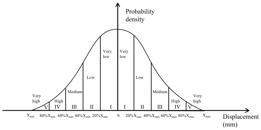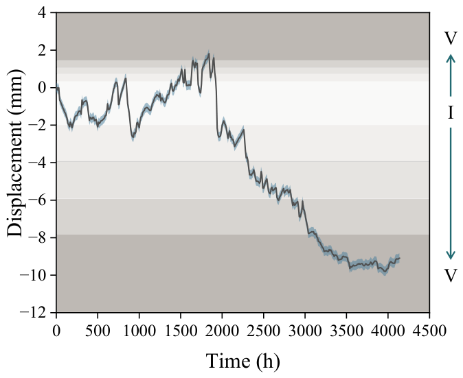The normality of the vault-displacement observations used for LHS parameter estimation was further examined using a normal Q–Q plot, as presented in Figure S3. On this basis, the probabilistic distribution of tunnel vault displacement was represented by a normal distribution for the subsequent LHS-based uncertainty propagation. Based on the predicted displacement statistics, LHS was employed to generate a large number of displacement realizations, which formed the basis for subsequent risk assessment. To express the predicted displacement magnitude in a project-specific form, a relative deformation-severity classification framework was established. Previous studies have demonstrated that intervals provide an effective and practical approach for risk evaluation in geotechnical systems. Following the percentage-based equal-width interval classification method proposed by Li et al. [33], the classification boundaries were established at 20%, 40%, 60%, and 80% of the respective extreme values of the positive and negative displacement ranges. The five categories were designated Levels I–V, corresponding to very low, low, medium, high, and very high relative deformation severity, respectively. These categories indicate the relative magnitude of tunnel vault displacement within the simulated range for the investigated case study. They do not represent universal engineering safety thresholds, probabilities of failure, structural safety states, or code-based warning levels. Project-specific design limits and engineering criteria should be used when formal safety decisions are required. The resulting classification is presented in

Table 7. Project-specific relative deformation-severity classification for tunnel vault displacement.

Risk Level	Risk Interval	Relative Deformation Severity
I	[−1.960, 0.365]	Very low
II	[−3.919, −1.960) ∪ (0.365, 0.730]	Low
III	[−5.879, −3.919) ∪ (0.730, 1.094]	Medium
IV	[−7.839, −5.879) ∪ (1.094, 1.459]	High
V	[−9.798, −7.839) ∪ (1.459, 1.824]	Very high

, and a schematic illustration of the five relative deformation-severity levels is provided in Figure 8.

Figure 9 presents the temporal evolution of the project-specific relative deformation-severity levels together with the corresponding 95% confidence interval. As the predicted displacement magnitude increases, the observations are assigned to progressively higher relative severity levels. These transitions indicate the position of the predicted displacement within the project-specific classification range and can support monitoring prioritization. Levels IV and V indicate relatively large displacement magnitudes and may warrant closer inspection; however, they do not independently demonstrate structural failure, an unsafe state, or an increased probability of failure. Any engineering intervention should therefore be determined using project-specific design limits, field observations, and professional engineering assessment.

The software implementation and engineering integration of the proposed framework are currently under development and have not yet been deployed in an operational tunnel-monitoring project. Ongoing and future work will focus on adapting the framework to project-specific monitoring conditions, evaluating its computational performance on target hardware, and developing it as a decision-support tool for engineering assessment.

5. Conclusions

This study developed an integrated framework for tunnel vault displacement prediction and uncertainty-informed relative deformation-severity assessment under complex geological conditions. Four prediction models were combined with GA, WOA, and PSO, producing 16 candidate models. Their predictive performance was evaluated using a chronological data partition, rolling validation, and statistical significance analysis. The principal conclusions are as follows.

• Hyperparameter optimization improved the predictive performance of the corresponding baseline models, although the improvement depended on both the optimization strategy and model architecture. PSO produced the most pronounced improvements, particularly when coupled with recurrent neural networks. Among the unoptimized models, Peephole-LSTM achieved the best performance, confirming the benefit of incorporating cell-state information into the gating mechanism.
• Among the 16 models evaluated under the same experimental protocol, PSO-Peephole-LSTM achieved the best testing-set performance, with an MAE of 0.058 mm, an RMSE of 0.074 mm, and an R² of 0.884. Its predictive advantage over the other 15 models was further supported by the rolling-validation results and statistical significance analysis. The original DCSGN study did not fully report or publicly provide all the materials required to reproduce its exact experimental conditions. Therefore, the models developed in this study could not be configured and evaluated under the same conditions as DCSGN. The literature-reported DCSGN results were consequently retained only as a contextual reference and excluded from the direct ranking and superiority assessment.
• The rolling-validation results provided evidence supporting the temporal robustness of PSO-Peephole-LSTM under the adopted expanding-window validation design. It achieved the lowest mean RMSE and the best average rank. The Friedman test identified significant overall differences among the 16 models. Subsequent Wilcoxon signed-rank tests with Holm correction indicated that PSO-Peephole-LSTM significantly outperformed the competing models under the adopted validation protocol.
• The LHS analysis generated 2000 displacement realizations from the PSO-Peephole-LSTM predictions. These realizations were used to establish five project-specific relative deformation-severity levels. The proposed levels provide a relative indication of displacement magnitude and can support monitoring prioritization within the investigated case study. They should not be interpreted as universal engineering safety thresholds, probabilities of failure, structural safety states, or code-based warning levels. Formal safety decisions should remain dependent on project-specific design limits and engineering assessment.