Seismic Event Detection in the Valencian Community Seismic Network Using the Wavelet Scattering Transform, PCA, and SVM: A Robust Lightweight Alternative to Deep Learning for Local Seismic Networks

Abstract

Southeastern Spain is a region of moderate-to-high seismic risk, where reliable seismic event detection is a prerequisite for earthquake early warning systems. This paper presents a seismic event detection pipeline based on the Wavelet Scattering Transform (WST) with a ZNE component-feature ensemble, Principal Component Analysis (PCA), and a Support Vector Machine (SVM), developed for the Valencian Community Seismic Network (SISCOVA) in Spain. The pipeline is evaluated on a local dataset of labeled three-component traces spanning January 2025 through mid-March 2026 and benchmarked against a classical recursive STA/LTA detector and three state-of-the-art pretrained deep learning models evaluated in a zero-shot transfer setting. Under known signal-to-noise ratio conditions, the proposed approach achieves an accuracy and F1-score of 98.82%, outperforming both the STA/LTA baseline and all evaluated deep learning models. Qualitative validation on continuous full-day recordings from the SISCOVA network further confirms its operational viability. These results demonstrate that WST-based feature extraction, combined with classical machine learning, provides an effective and computationally efficient alternative for seismic event detection in local seismic networks.

1. Introduction

Southeastern Spain is one of the areas with the highest seismic risk on the Iberian Peninsula, as a result of the collision between the Eurasian and African tectonic plates [1,2]. From 1500 to the present, this area has experienced 10 earthquakes with maximum intensities between IX and X on the MSK scale, the largest recorded event being the 1910 Adra earthquake (Mw 6.1) [3,4]. The Bajo Segura depression, in the province of Alicante, is characterized by moderate seismicity with historical events of great magnitude [5,6,7,8]. The significant demographic and economic growth experienced by this region since the 1990s, combined with the characteristics of the basin’s soil and ongoing seismic activity, make this entire area one of moderate-to-high seismic risk, where earthquake early warning and site response studies are crucial for reducing the number of casualties and economic damage.

Within seismic risk reduction, three types of actions can be distinguished based on their time scales: Operational Earthquake Forecasting (OEF), Earthquake Early Warning (EEW), and Rapid Response to Earthquakes (RREs) [9]. EEW systems aim to provide real-time information about an ongoing earthquake before its arrival, so that the public and relevant agencies can take protective measures before seismic ground motion reaches populated areas. This strategy helps reduce disaster risk and increase resilience to seismic hazards in urban environments.

EEW systems are based on two complementary physical principles: information in the form of electromagnetic waves travels faster than seismic waves (which are mechanical waves), and most of the destructive energy of an earthquake is carried by S-waves and surface waves, which arrive after the faster but lower-amplitude P-waves. This time interval, which can range from a few seconds to several minutes depending on the distance from the epicenter, allows for the issuance of alerts with sufficient advance notice to reduce the impact of the event on multiple sectors of society.

The traditional approach to early earthquake warning has been to transmit all data from the seismic stations to a central monitoring system, where signal processing is carried out either through automated methods or manually by qualified specialists to generate alerts. This is the operating principle used today at the Valencian Community Seismic Network (SISCOVA), in the southeastern region of Spain. However, in recent years, with the rise of the Internet of Things (IoT) and edge computing paradigms, it has become increasingly common to process signals directly at the sensor nodes of the seismic networks, and to transmit the estimated parameters and the alert to the central monitoring system [10,11,12]. This approach significantly reduces the alert times and extends the response time window in case of seismic events [9,13,14].

A prerequisite for any EEW system is a reliable, low-latency detector capable of discriminating seismic events from the background noise. To perform this task in real time at the station hardware level, prominent lightweight approaches that can operate continuously on raw waveform data are required on resource-constrained hardware.

Automatic seismic event detection has been addressed by a succession of approaches of increasing complexity. Traditional detection methods were based on deterministic approaches. The Short-Term Average/Long-Term Average (STA/LTA) algorithm remains the canonical classical method, exploiting the rapid onset of seismic energy as a transient-to-background energy ratio at the time of first arrival of the P waves [15]. Its computational simplicity and real-time capability have made it ubiquitous in operational seismic networks, and so it has been used in the SISCOVA network [16]. However, STA/LTA-based detectors are inherently sensitive to the threshold parameter and exhibit elevated false alarm rates in the presence of transients or impulsive noise sources. Other alternatives involve criteria based on the estimation of statistical parameters like kurtosis in the signals [17].

The introduction of machine learning to seismological signal processing has led to significant improvements in detection reliability [18]. Early feature engineering approaches demonstrated that hand-crafted spectral and time-domain descriptors fed to classical machine learning classifiers could provide discrimination between seismic events and noise that surpasses the mentioned classic methods [19,20]. Among them, the use of wavelet-domain representations has been explored as a means of capturing the multi-scale frequency-time structure of seismic signals in the form of highly discriminative features [21,22].

Various feature engineering methods based on the Continuous Wavelet Transform (CWT) and Wavelet Packet Decomposition (WPD) have been proposed to characterize non-stationary seismic signals [20,23,24]. However, the effectiveness of these descriptors is fundamentally limited by the subjectivity and complexity involved in selecting an appropriate mother wavelet, a process that typically relies on trial-and-error or specific stability metrics that often fail to generalize across massive datasets [23,25,26,27,28]. While adaptive approaches such as the Empirical Wavelet Transform (EWT) attempt to mitigate the rigidity of predefined wavelet bases by designing filter banks according to the signal’s spectral support, these methods remain sensitive to segmentation hyperparameters and translations in signals belonging to the same class [28].

More recently, deep learning architectures have achieved the current state-of-the-art performance on large-scale global and regional benchmarks [29,30,31]. Some of the most prominent architectures established are PhaseNet [32], the EQTransformer [33], and CRED [34], which are sequence-to-sequence models trained on large datasets of labeled waveforms acquired globally. These have also spawned other models oriented to domain-specific tasks inside the broader scope of seismology [35]. Nevertheless, the generalization of these powerful deep learning models to local networks with different geological settings, noise environments, or sensor characteristics is not guaranteed, and performance degradation under domain shift to specific regions has been documented in the literature [36,37]. This suggests that the use of these models in local contexts without fine-tuning or specific domain adaptation compromises the quality of the results obtained by their use, which is a highly data-demanding task non-viable for local seismic networks with limited data availability and reduced event catalogs. Moreover, the high parametric complexity of deep learning models makes them more difficult to deploy directly on resource-constrained embedded hardware than other machine learning solutions.

The use of wavelet-based features coupled with deep learning architectures has also been explored to enhance the representational capacity of neural networks [38]. In these cases, the reliance on an external, fixed feature engineering stage results in a significant decoupling from the learning process, necessitating a prerequisite batch conversion of signals that prevents the dynamic, end-to-end optimization of discriminative features within modern deep learning architectures.

In 2013, Bruna and Mallat proposed the Wavelet Scattering Transform (WST) as a method for learning representation and feature extraction from signals [39]. The WST is a mathematical operator that generates representations that are invariant to time translations and robust to local signal deformations, properties that make it a very useful tool for extracting highly discriminative features in classification tasks [40]. It is constructed through the iterative application of banks of wavelet filters followed by a modulus operator and a low-frequency averaging filter, operations similar to those found in a convolutional neural network. This is why the WST can be interpreted as a convolutional neural network, usually named a wavelet scattering network, where the filters in the convolutional layers are predefined wavelets, rather than being learned through a training process from source data, as occurs in deep learning models. This allows for obtaining a robust yet interpretable and sparse feature representation that can be used to feed machine learning classifiers that are much simpler than complex deep learning architectures and able to achieve similar performance with considerably less data. The use of WST features has provided prominent results in tasks like audio signal classification, biomedical signal processing, and vibration analysis [41,42,43].

The WST has also been explored in seismological signal processing. In the works of Fan et al. [44] and Xin et al. [45], the WST is used with a support vector machine (SVM) classifier for the automatic recognition of microseismic events induced by rock fractures in coal mines using low-SNR single-component signals from short-range industrial monitoring environments. While these works provide a useful insight into the discriminative power of wavelet scattering features for seismic signal classification, their geological and operational context differs from that of earthquake monitoring applications, as coal mine microseismic monitoring targets higher-frequency (>10 Hz) stress-fracture events in confined underground environments. In addition to this, the detection algorithm they propose was only compared against a classical STA/LTA detector, which is already known to have several limitations for its use in real-world environments. Moreover, the validation tests in these works are conducted on very limited data, collected in controlled industrial settings with known sources.

In the scope of seismic event detection methods targeting edge computing environments, the broader field of seismic monitoring has moved toward the development of lightweight deep learning architectures explicitly designed for on-device processing [11,46,47]. Recent models such as LightEQ [11] and SeismicSense [47] employ a two-stage hierarchical pipeline where a recursive STA/LTA pre-filter acts as a triggering mechanism for quantized neural networks, effectively reducing the frequency of power-intensive inference tasks on microcontrollers. However, these approaches encounter a fundamental trade-off between model compression and temporal resolution; for instance, reducing the output prediction vector through aggressive striding in convolutional layers significantly hinders the detection of short-duration seismic signals [46]. To mitigate information loss during downsampling, architectures like ICAT-net [48] have introduced space-to-depth (SPD-Conv) transformations and coordinate attention modules to preserve fine-grained feature arrangements. Similarly, LEQNet [49] and LFTNet [50] utilize depthwise separable convolutions and recursive structures to achieve parameter reductions of up to 88% compared to state-of-the-art benchmarks like EQTransformer. Despite these advances, a significant limitation persists: current lightweight models remain largely dependent on massive global datasets, which fail to capture the local geological variability and site-specific noise floor characteristics critical for decentralized local networks.

In this paper, we propose an algorithmic pipeline for seismic event detection (including earthquakes and anthropogenic sources such as quarry blasts) in local earthquake monitoring. The proposed pipeline combines wavelet scattering-based feature extraction with classical machine learning techniques for seismic event detection. The proposed method is intended to address both the data limitation problem of the SISCOVA network in Spain and the need for lightweight, robust alternatives for seismic event detection over the seismic stations’ available hardware in the path to achieve a low-latency earthquake early warning system.

Therefore, the main contributions of this paper are:

• Algorithm innovation: A seismic event detection pipeline combining Wavelet Scattering Transform (WST) feature extraction with a ZNE component-feature ensemble, Principal Component Analysis (PCA) for dimensionality reduction, and Support Vector Machine (SVM) classification.
• Dataset construction: A new, manually confirmed dataset of seismic events and noise built from the SISCOVA network catalog, comprising 772 local earthquake and quarry blast events recorded between January 2025 and March 2026. The dataset is released as a resource for other researchers working on seismic event signal processing in the region.
• Regional zero-shot benchmarking: A zero-shot evaluation of three state-of-the-art deep learning models (PhaseNet, EQTransformer and CRED) on data from the Valencian Community Seismic Network, establishing a baseline of their out-of-domain performance for local earthquake detection in this region. To the knowledge of the authors, none of these models’ performance has been tested exclusively on data from the Valencian Community, even though in [51] the authors experimented with some of them for seismic phase picking using data from another seismic network located on the eastern coast of Spain, which constitutes a precedent.

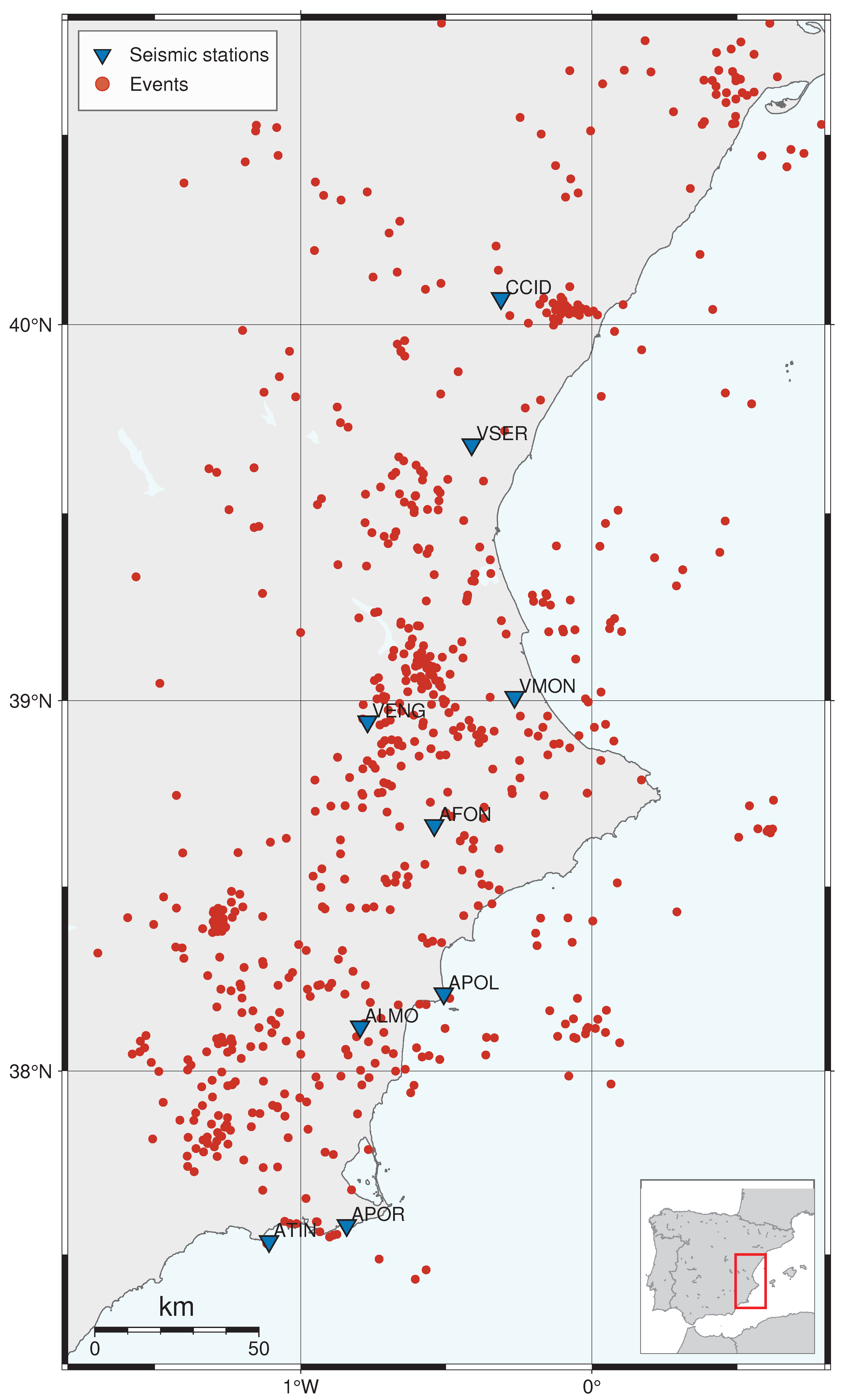
The remainder of this paper is organized as follows: Section 2 describes the mathematical fundamentals of the methods used in the proposal; Section 3 describes the SISCOVA network and the dataset construction procedure; Section 4 details the proposed algorithmic pipeline; and Section 5 defines the experimental workflow followed, presents the quantitative results and provides a comparative analysis with other methods, contextualizing the findings within the broader literature. It also describes the qualitative validation of the proposed pipeline performed using continuous full-day recordings taken from selected days with representative seismic activity. Finally, the conclusions summarize the main findings and outline future work directions.

2. Theoretical Background

2.1. Wavelet Scattering Transform (WST)

The Wavelet Scattering Transform (WST) was developed to address fundamental limitations inherent in classical signal processing techniques and modern deep learning architectures. Traditional Fourier transforms are globally time-invariant but remain unstable to deformations at high frequencies [40]. While classical wavelet transforms provide multi-resolution characteristics and stability against signal deformations, they lack translation invariance when subsampling is involved [52]. Consequently, minor shifts in the input signal can lead to significant variations in the extracted features.

In deep learning, convolutional neural networks (CNNs) have become the dominant architecture for feature extraction. However, the convolutional kernels of a CNN are free parameters estimated by empirical risk minimization, and standard generalization theory indicates that the resulting excess risk scales with the network’s effective capacity relative to the number of training samples; with tens to hundreds of thousands of trainable filter weights, this capacity is large, so CNNs require considerably large training sets to avoid overfitting, and their noise-suppression behavior is itself learned rather than guaranteed, making it unreliable when the training data offers limited exposure to noise diversity, as is the case for small local datasets. The WST addresses these limitations by serving as a knowledge-based feature extractor that possesses a structure similar to a deep CNN, but replaces the learned kernel filters with predefined wavelet filters, eliminating the associated estimation variance entirely. Because this filter bank is fixed by design rather than fit to data, its stability to noise and deformation is analytically guaranteed independently of the training set. This allows the WST to work accurately and efficiently with small local datasets while maintaining the advantages of deep architectures, such as multi-scale contraction and linearization of hierarchical symmetries.

The WST is defined as a recursive cascade of wavelet transforms followed by a nonlinear modulus operator and a low-pass spatial averaging filter. The transformation is built upon a family of wavelets ${\psi }_{\lambda }$ generated by dilating and translating a mother wavelet $\Psi$. The Morlet wavelet is typically used due to its optimal joint concentration in the time-frequency plane, which allows it to provide an excellent compromise between time and frequency resolution [53]. 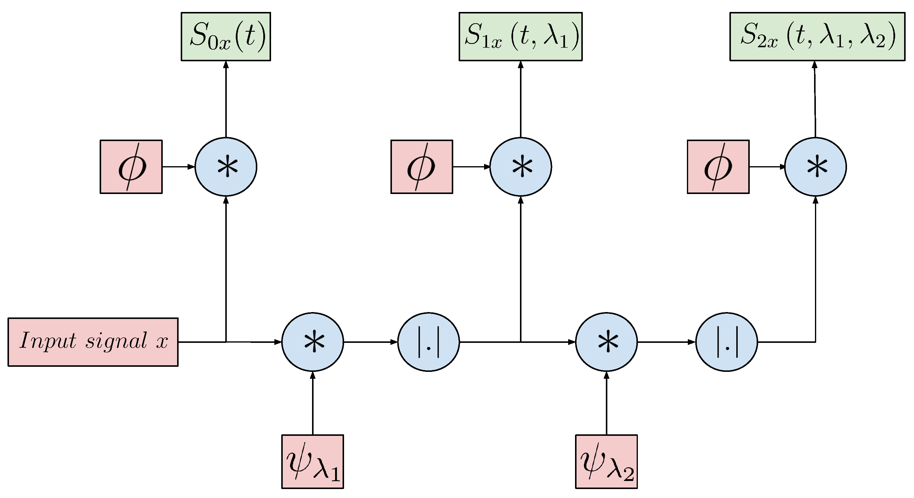Figure 1 shows a block diagram of a Wavelet Scattering Transform with two scattering layers.

The transform begins with the zero-order scattering coefficient, $S_{0x}\left(t\right)$, which represents the local translation-invariant descriptor of the signal x obtained through a low-pass Gaussian filter $\varphi$:

$$S_{0x}\left(t\right)=|x\ast \varphi \left(t\right)|$$

(1)

While this step provides invariance, it removes all high-frequency information. To recover this information, the signal is convolved with a high-frequency wavelet filterbank in the first layer composed of wavelets ${\psi }_{{\lambda }_1}$ and subjected to a complex modulus operator to remove phase oscillations:

$$U_{1x}(t,{\lambda }_1)=|x\ast {\psi }_{{\lambda }_1}\left(t\right)|$$

(2)

The first-order scattering coefficients are then computed by smoothing this result with the low-pass filter:

$$S_{1x}(t,{\lambda }_1)=U_{1x}(t,{\lambda }_1)\ast \varphi \left(t\right)=|x\ast {\psi }_{{\lambda }_1}\left(t\right)|\ast \varphi \left(t\right)$$

(3)

To capture high-frequency details lost in the first stage, the process is repeated on the first-order propagator $U_{1x}$ using a second wavelet filterbank with wavelets ${\psi }_{{\lambda }_2}$. The second-order scattering coefficients are therefore defined as follows:

$$S_{2x}(t,{\lambda }_1,{\lambda }_2)=U_{2x}(t,{\lambda }_1,{\lambda }_2)\ast \varphi \left(t\right)=||x\ast {\psi }_{{\lambda }_1}(t\left)\right|\ast {\psi }_{{\lambda }_2}\left(t\right)|\ast \varphi \left(t\right)$$

(4)

At the end, the first-order scattering coefficients capture information related to the signal energy in each frequency band, while the second-order scattering coefficients encode information related to the amplitude modulation of the envelope [40]. Higher-order implementations with more layers are proven to be unnecessary for most applications, as the energy in higher orders becomes negligible and the computational complexity increases exponentially.

The wavelet scattering network architecture is defined by two parameters: the invariance scale $T=2^J$ that defines the temporal support for the low-pass filter and the number of wavelets per octave for each wavelet filterbank Q. This means that the center frequencies of the wavelets for every filterbank are given by $\lambda =2^{k/Q}$ for $k\in \mathbb{Z}$ on a normalized frequency axis. The bandwidth of the normalized wavelets $\widehat{\psi }$ is of the order of $Q^{-1}$, to cover the whole frequency axis with these band-pass wavelet filters. The support of ${\widehat{\psi }}_{\lambda }\left(\omega \right)$ is centered in $\lambda$ with a frequency bandwidth $\lambda /Q$, whereas the energy of ${\psi }_{\lambda }\left(t\right)$ is concentrated around 0 in an interval of size $2\pi Q/\lambda$. To guarantee that this interval is smaller than the time invariance scale T, ${\psi }_{\lambda }$ is defined as ${\psi }_{\lambda }\left(t\right)=\lambda \psi \left(\lambda t\right)$ and hence ${\widehat{\psi }}_{\lambda }\left(\omega \right)=\widehat{\psi }(\omega /\lambda )$ for $\lambda \ge 2\pi Q/T$. For $\lambda <2\pi Q/T$, the lower-frequency interval $[0,2\pi Q/T]$ is covered with about $Q-1$ equally spaced filters ${\widehat{\psi }}_{\lambda }$ with constant frequency bandwidth $2\pi /T$. For simplicity, these lower-frequency filters are still called wavelets [40]. The low-pass filter $\varphi$ is then defined as a scaled Gaussian window ${\varphi }_{2^J}\left(t\right)=2^{-2J}\varphi \left(2^{-J}t\right)$ with a frequency bandwidth of approximately $2\pi /T$ whose response $|\widehat{\varphi }{\left(\omega \right)|}^2$ is mathematically constrained by the Littlewood–Paley condition [39].

By employing this cascade of wavelet convolutions, complex modulus nonlinearities, and local averaging, the WST generates signal representations that are translation-invariant, stable to local deformations (such as time-warping), and robust against noise.

2.2. Principal Component Analysis (PCA)

Principal component analysis (PCA) is a well-established technique for dimensionality reduction, which has evolved from its classical formulation to domain-specific variations [54]. PCA is a multivariate statistical method that combines information from several variables observed on the same subjects into fewer variables, transforming a set of p observed variables into a smaller set of r linear combinations called principal components (PCs). These maximally explain the variance of all the variables. In the process, the method aims to project the original data into a lower-dimensional space such that the major part of the total variance is optimally explained [55].

The first principal component, $P{C}_1$, is derived as a linear combination of the original variables that maximizes the variance across the n sampling units. Successive components are sought to explain the maximum possible residual variance left unexplained by previous components, subject to the constraint that each new PC must be uncorrelated with all preceding PCs. This orthogonality ensures that each component measures a distinct feature of the data structure. The process may continue until the number of PCs equals the number of variables, at which point 100% of the total variance is accounted for.

The computation of principal components can be achieved through the singular value decomposition (SVD) [56]. The SVD decomposes a column-centered data matrix X of n rows and p columns into three matrices:

$$X=UD{V}^T$$

(5)

where D is a diagonal matrix containing positive singular values (${\alpha }_1,{\alpha }_2,\dots$) in descending order, and U and V are orthonormal matrices of left and right singular vectors, respectively. The right singular vectors (columns $v_k$) are identical to the eigenvectors of the covariance matrix of the data. The squared singular values, when the data matrix is rescaled by $1/\sqrt{n}$, are equivalent to the variances (eigenvalues ${\lambda }_k$) explained by each dimension.

Written as a sum of products of the individual vectors, the SVD of X is ${\sum }_{k=1}^m{\alpha }_k{u}_k{v}_k^T$, where m is the rank of X. Since the sum of squares of each rank-1 matrix $u_k{v}_k^T$ is equal to 1 and the singular values are in descending order, this suggests that taking the first terms of the sum will give an approximation to X.

The principal component analysis coordinates in r dimensions are in the first r columns of $UD$, and the principal coordinates are in the first r columns of V. For a new observation $x_{\mathrm{n}}\in {\mathbb{R}}^p$, the PCA scores are obtained after centering with the same training criteria by projecting onto the retained right singular vectors $V_r\in {\mathbb{R}}^{p\times r}$:

$$y_{\mathrm{n}}=x_{\mathrm{n}}{V}_r\in {\mathbb{R}}^r.$$

(6)

where $y_n\in {\mathbb{R}}^r$ is the dimensionality-reduced observation in the r-dimensional subspace.

2.3. Support Vector Machines (SVM)

Support Vector Machines (SVM) are a supervised machine learning method that classifies objects by representing them as points in an N-dimensional feature space. Its primary objective is to identify the “best hyperplane” or decision boundary that splits the feature space into classes, maximizing the “gap” or distance between them [57].

The hyperplane used as the decision boundary is defined as [58]:

$$\mathbf{w}·\mathbf{x}+b=0$$

(7)

where $\mathbf{w}\in {\mathbb{R}}^n$ is the weight vector, $\mathbf{x}\in {\mathbb{R}}^n$ is a feature vector, and b is the bias term specifying the offset of the hyperplane from the origin. Geometrically, $\mathbf{w}$ is the normal vector to the hyperplane. For any two data points ${\mathbf{x}}_1,{\mathbf{x}}_2\in {\mathbb{R}}^n$ satisfying (7), $\mathbf{w}·({\mathbf{x}}_1-{\mathbf{x}}_2)=0$, as $\mathbf{w}$ is orthogonal to every vector lying within the hyperplane. As a consequence, the unitary vector $\mathbf{w}/\parallel \mathbf{w}\parallel$ fixes the orientation of the decision boundary in the feature space, while b governs its position, translating the hyperplane along the direction of $\mathbf{w}$ without altering its orientation.

For an arbitrary point $\mathbf{x}$, the signed distance to the hyperplane is given by the following:

$$d\left(\mathbf{x}\right)={\displaystyle \frac{\mathbf{w}·\mathbf{x}+b}{\parallel \mathbf{w}\parallel }}$$

(8)

whose sign indicates on which side of the hyperplane $\mathbf{x}$ lies and whose magnitude gives the Euclidean distance to it. This quantity is the geometric justification for the SVM decision function:

$$f\left(\mathbf{x}\right)=sign(\mathbf{w}·\mathbf{x}+b)$$

(9)

which assigns the predicted label $\widehat{y}\in \{-1,+1\}$ according to the side of the hyperplane on which $\mathbf{x}$ falls, independent of the distance normalization in (8).

Because the pair $(\mathbf{w},b)$ in (7) is defined only up to a positive scalar multiple—any $(\lambda \mathbf{w},\lambda b)$ with $\lambda >0$ describes the same hyperplane—this scaling freedom is conventionally resolved by adopting the canonical form, in which $\mathbf{w}$ and b are scaled such that the nearest training points of each class satisfy $\mathbf{w}·{\mathbf{x}}_i+b=y_i$ for ${\mathbf{x}}_i$ on the margin boundary, i.e., $\mathbf{w}·{\mathbf{x}}_i+b=\pm 1$. This normalization fixes $\parallel \mathbf{w}\parallel$ relative to the training data and provides the geometric scaffold upon which the margin-maximization formulation is subsequently constructed.

Given the canonical hyperplane convention, the two boundary hyperplanes $\mathbf{w}·\mathbf{x}+b=1$ and $\mathbf{w}·\mathbf{x}+b=-1$ delimit the margin within which no training point lies. The perpendicular distance between these parallel hyperplanes follows directly from (8) and is given by

$$\mathrm{margin}={\displaystyle \frac{2}{\parallel \mathbf{w}\parallel }}.$$

(10)

Maximizing this margin is therefore equivalent to minimizing $\parallel \mathbf{w}\parallel$, or equivalently ${\parallel \mathbf{w}\parallel }^2$ for analytical convenience, subject to the constraint that every training point lies on or beyond its respective boundary hyperplane. For a labeled training set ${\left\{({\mathbf{x}}_i,y_i)\right\}}_{i=1}^N$ with $y_i\in \{-1,+1\}$, this constraint is written compactly as $y_i(\mathbf{w}·{\mathbf{x}}_i+b)\ge 1$ for all i, yielding the hard-margin optimization problem:

$$\underset{\mathbf{w},b}{min}{\displaystyle \frac{1}{2}}{\parallel \mathbf{w}\parallel }^2\mathrm{subject}\mathrm{to}{y}_i(\mathbf{w}·{\mathbf{x}}_i+b)\ge 1,i=1,\dots ,N.$$

(11)

This formulation presumes linear separability in the feature space, an assumption rarely satisfied in practice. To accommodate cases of nonlinear separability, slack variables ${\xi }_i\ge 0$ are introduced for each training instance, relaxing the strict margin constraint to $y_i(\mathbf{w}·{\mathbf{x}}_i+b)\ge 1-{\xi }_i$. Each ${\xi }_i$ quantifies the degree to which ${\mathbf{x}}_i$ is permitted to violate the margin, either by lying within the margin region ($0<{\xi }_i\le 1$) or on the incorrect side of the decision boundary (${\xi }_i>1$). This relaxation gives rise to the soft-margin primal objective.

$$\underset{\mathbf{w},b,\xi }{min}{\displaystyle \frac{1}{2}}{\parallel \mathbf{w}\parallel }^2+C{\displaystyle \sum _{i=1}^N}{\xi }_i,$$

(12)

subject to $y_i(\mathbf{w}·{\mathbf{x}}_i+b)\ge 1-{\xi }_i$ and ${\xi }_i\ge 0$ for all i.

The regularization parameter $C>0$ governs the trade-off between the two competing terms in (12): the margin-maximization term ${\displaystyle \frac{1}{2}}{\parallel \mathbf{w}\parallel }^2$, which favors a wide margin and thus better generalization, and the empirical risk term $C{\sum }_i{\xi }_i$, which penalizes margin violations and training misclassifications. A small value of C tolerates greater cumulative slack in exchange for a wider margin, yielding a smoother decision boundary less sensitive to individual noisy or overlapping samples; a large value of C enforces stricter adherence to the separability constraints, at the risk of overfitting to outliers within the training distribution. This trade-off manifests in the dual formulation as a box constraint on the Lagrange multipliers in the optimization problem solution, $0\le {\alpha }_i\le C$, bounding the influence of individual support vectors on the resulting decision function.

Whereas the soft-margin formulation in (12) accommodates non-separability through slack, it retains an implicit assumption of approximate linear separability in the input feature space. When the underlying class distributions exhibit genuinely nonlinear decision boundaries, a linear hyperplane in the original feature space may be insufficient regardless of the value of C. The kernel trick addresses this limitation by implicitly mapping the input space to a higher-dimensional feature space via a nonlinear transformation $\varphi :{\mathbb{R}}^n\to \mathcal{H}$, in which a linear separating hyperplane, of the form already established in (9), can more effectively partition the transformed data features.

Direct computation of $\varphi \left(\mathbf{x}\right)$ is generally intractable for a high-dimensional $\mathcal{H}$. However, because both the dual formulation of (10) and (12) and the resulting decision function depend on the training data only through pairwise dot products, this dependence can be replaced by a kernel function K defined as follows:

$$K({\mathbf{x}}_i,{\mathbf{x}}_j)=\varphi \left({\mathbf{x}}_i\right)·\varphi \left({\mathbf{x}}_j\right)$$

(13)

which computes the inner product in $\mathcal{H}$ without explicit evaluation of $\varphi$.

In the kernel expression $K({\mathbf{x}}_i,{\mathbf{x}}_j)=\varphi \left({\mathbf{x}}_i\right)·\varphi \left({\mathbf{x}}_j\right)$, ${\mathbf{x}}_i$ and ${\mathbf{x}}_j$ are two feature vectors drawn from the training set $\{{\mathbf{x}}_1,\dots ,{\mathbf{x}}_N\}$. The kernel is evaluated pairwise over the training set to build the $N\times N$ Gram matrix, where entry $(i,j)$ gives $K({\mathbf{x}}_i,{\mathbf{x}}_j)$ for every pair of training samples. This matrix is what’s used in the dual optimization to solve for the ${\alpha }_i$ coefficients.

The decision function of (9) generalizes accordingly to:

$$f\left(\mathbf{x}\right)=sign\left({\displaystyle \sum _{i=1}^N}{\alpha }_i{y}_{i}K({\mathbf{x}}_i,\mathbf{x})+b\right)$$

(14)

where ${\alpha }_i$ are the Lagrange multipliers bounded by $0\le {\alpha }_i\le C$ as introduced previously, and the summation is restricted in practice to the support vectors for which ${\alpha }_i>0$.

In the decision function, ${\mathbf{x}}_i$ ranges over the support vectors (the training points with ${\alpha }_i>0$), while $\mathbf{x}$ is the new, unlabeled feature vector being classified. So at inference time, the kernel similarity $K({\mathbf{x}}_i,\mathbf{x})$ is computed between each stored support vector and the new sample.

Commonly employed kernels include the linear kernel, the polynomial kernel, and the Gaussian radial basis function (RBF) kernel. The kernel selection is data-dependent. For high-dimensional data with complex intrinsic relations, the RBF kernel is generally preferred [59,60,61]. It is defined as follows:

$$K({\mathbf{x}}_i,{\mathbf{x}}_j)=e^{-\gamma {\parallel {\mathbf{x}}_i-{\mathbf{x}}_j\parallel }^2}$$

(15)

The RBF kernel induces an infinite-dimensional feature space and introduces an additional hyperparameter $\gamma$ controlling the locality of influence of each support vector.

3. Database

3.1. Valencian Community Seismic Network (SISCOVA)

The Valencian Community Seismic Network (SISCOVA) is a seismic network developed by the Cartographic Institute of Valencia in collaboration with the Valencian Regional Government’s Agency for Safety and Emergency Response, the University of Alicante, and the Provincial Councils of Castellón and Alicante. This network is managed by the Seismic Recording Unit at the University of Alicante, under a collaboration agreement signed between the Cartographic Institute of Valencia and the University of Alicante in 2022. This collaboration expanded the university’s seismic network and allowed it to cover the entire territory of the Valencian Community [62].

Currently, the SISCOVA network has 23 recording devices installed within the area where seismic activity is monitored, which covers the autonomous region plus a 100-km buffer zone around its geographical boundaries. The network of seismic stations consists of 9 broadband seismometers, whose primary objective is to detect all seismic activity that occurs, regardless of the magnitude of the events; 9 hybrid stations, which enable the detection of medium-sized events (using short-period velocity sensors) and the recording of acceleration signals (using acceleration sensors) caused by larger earthquakes; and 6 accelerometers, which, together with the hybrid stations, form the Valencian Community’s Accelerometer Network for the detection of strong ground motion.

The data used in this study correspond to seismic events that occurred from January 2025 through mid-March 2026 and were recorded by the SISCOVA network’s broadband seismic stations. Only those events that have been manually confirmed by both specialists from the Seismic Recording Unit at the University of Alicante and the IGN (National Geographic Institute of Spain) were included. The data were downloaded from the SISCOVA network’s SeisComP server and stored in a public repository [63], where the following files and folders are located:

• siscovap_inv.xml: network inventory file
• Records_Year_StartMonth_to_EndMonth: folders containing the event catalogs downloaded from the SeisComP server by quarter. Each folder contains two subfolders:

  –

  earthquakes: contains the catalogs of earthquake events

  –

  quarryBlast: contains the catalogs of quarry blast events

  Inside each subfolder, there is an .xml file for each event that contains all the information related to the event in the form of metadata, as well as a miniSEED (.mseed) file containing the time series data recorded by the stations for that event. In addition, a .csv file is included with a summary table containing the essential metadata for the events in the subfolder.

Some details regarding the recorded signals of the events in the .mseed files in the earthquakes and quarryBlast source directories are:

• The time windows of the recorded signals for each event were taken from 1 min before the event’s origin time to 2 min after the origin time.
• The origin time is determined when performing the event location in SeisComP using the LOCSAT algorithm [64], and the time windows for all stations that recorded the event are referenced to that specific time.

The resulting data include records from the seismic network stations illustrated in

Table 1. Seismological stations from the SISCOVA network used in the study.

Network and Station Code	Location	Type of Installation	Sensor and Data Logger Equipment
ES.AFON	Font Roja Sanctuary	Seismic trench	Gluralp CMG-6TD (integrated digitizer)
VB.ALMO	Almoradí Ecomuseum	Seismic trench	Nanometrics Trillium Compact with Centaur–3 (CTR4-3S) digitizer
VB.APOL	Santa Pola Marine Research Center	Seismic trench	Guralp CMG-6TD (integrated digitizer)
VB.APOR	Cabo de Portman Lighthouse	Lighthouse base	Gluralp CMG-6TD (integrated digitizer)
VB.ATIN	Cabo Tiñoso Lighthouse	Lighthouse base	Gluralp CMG-6TD (integrated digitizer)
VB.CCID	Lucena del Cid Forest Observatory	9-m borehole	Nanometrics Trillium Compact with Centaur–3 (CTR4-3S) digitizer
VB.VENG	Enguera Airfield	Seismic trench	Nanometrics Trillium Compact with Centaur–6 (CTR4-6S) digitizer
VB.VMON	Mondúver Forest Observatory	Observatory base	Nanometrics Trillium Compact with Centaur–6 (CTR4-6S) digitizer
VB.VSER	Alto del Pino (Serra) Forest Observatory	Observatory base	Nanometrics Trillium Compact with Centaur–6 (CTR4-6S) digitizer

, which are equipped with HHZ, HHN, and HHE 3-component broadband channels, high-gain velocity sensors, and a sampling rate of 100 Hz.

Figure 2 shows the geographic distribution of the events and the seismological stations used in the study.

3.2. Data Conditioning and Dataset Construction

To organize the data from the sources in a standardized manner and facilitate further processing, the SeisBench standard was adopted for dataset creation from the available event data [65]. The choice of SeisBench is due, among other reasons, to its compatibility with the ObsPy framework [66], and to the fact that it provides a large number of easy-to-use Python tools and utilities for processing seismic event datasets in a uniform manner, while also integrating a large number of pretrained deep learning models that are already established as state-of-the-art for performing event detection, phase identification, or noise removal tasks. This greatly facilitates the evaluation of many of the solutions established with good results in the scientific literature on the data obtained from the SISCOVA seismic network, and allows for the evaluation of new solutions using the same conventions to perform comparisons.

To generate a SeisBench dataset, a standalone software script was designed in Python. This script constructs a SeisBench dataset by processing all the source data. It receives two directory trees of XML catalogs (‘.xml’) and MiniSEED waveforms (‘.mseed’)—one for earthquakes, one for quarry blasts—and for each event-station pair extracts two 60-s windows: a signal window containing the event, centered on the Pg-phase arrival sample ($-30$ s to +30 s) and a pre-event noise window ($-60$ s to 0 s). The window size used was 60 s to keep the samples in the dataset compatible with the longest window size used by SeisBench models. Figure 3 illustrates how the event and noise windows are obtained from the original seismic recordings, using as an example the vertical component recorded at the Lucena del Cid Forest Observatory station (station code CCID) for the earthquake event vb2025eyftu.

Before windowing, the script performs high-pass filtering of the waveforms with a cutoff frequency of 2.0 Hz to remove the DC and low-frequency trends, and computes an estimate of the signal-to-noise ratio (SNR) on the vertical component using the RMS values of window intervals containing pre-event noise and the event content. The SNR result is stored as metadata. For the noise and event RMS computation, the intervals used are $-30$ s to $-5$ s relative to the Pg arrival for the noise, to ensure a 5 s interval of margin prior to the Pg arrival and ensure the content of the interval is purely noise, and the 15 s next to the Pg arrival for the event. This latter interval length was selected taking into account that this is the approximate highest duration of most of the events recorded. Moreover, only signals from the first 3 stations at which each event was recorded were selected to create the dataset, in order to ensure that the events were sufficiently observable within the signal windows, avoiding the leakage of events located too far from the stations that may have arrived with a significant loss of energy.

Events are split into train/test partitions in an 80:20 ratio, stratified at the event level (not the trace level) to prevent data leakage, with a fixed random seed for reproducibility. The final output is a pair of files—metadata.csv containing per-trace attributes such as event identifiers, station codes, phase arrival samples, SNR, split assignment and class label, and waveforms.hdf5 storing the corresponding three-component waveform arrays in ZNE order—which together constitute a SeisBench-compatible dataset ready for direct consumption by machine learning pipelines. This resulted in a dataset with the class and sample distribution shown in

Table 2. Composition of the created SeisBench dataset.

Category	Training Samples	Test Samples
Event	1169	320
Noise	1169	320
Total samples	2338	640

.

4. Proposed Method

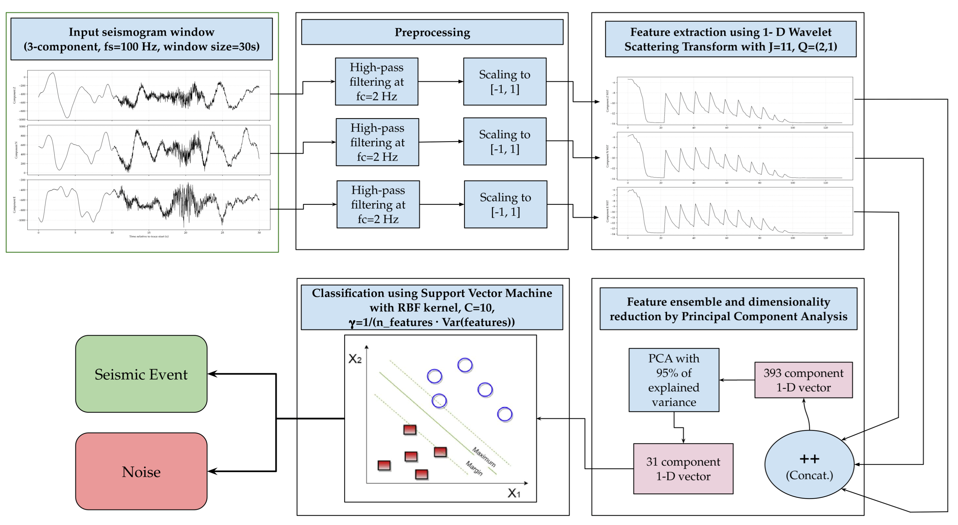
The proposed seismic event detection pipeline is illustrated in Figure 4. The pipeline consists of four main stages: preprocessing of data, feature extraction, dimensionality reduction, and classification.

In the following subsections, each of the stages is described in detail.

4.1. Preprocessing of Data

The first stage of processing involves applying a high-pass filter with a cutoff frequency of $f_c=2.0$ Hz to the seismic signal traces. The goal is to attenuate the low-frequency microseismic noise and long-period trends present in the signals, which do not provide discriminative information and may mask the relevant characteristics of the events. Next, to avoid biases in the computation of feature vectors caused by amplitude differences between traces, the traces are scaled to the interval $[-1,1]$.

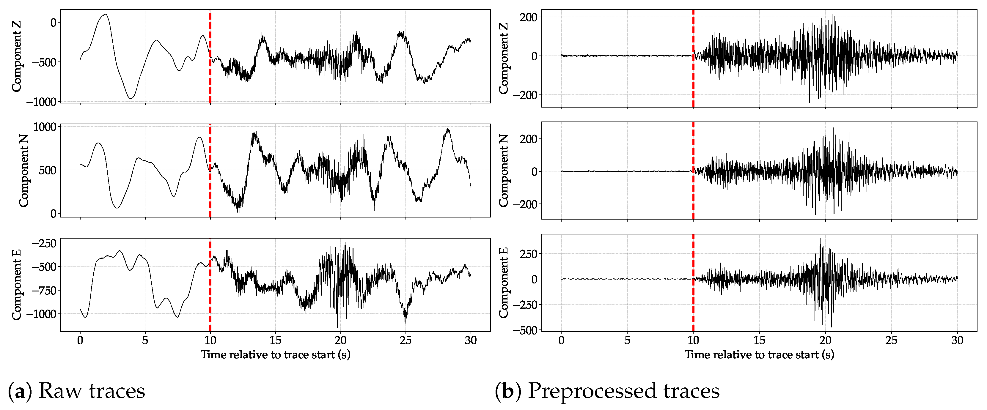
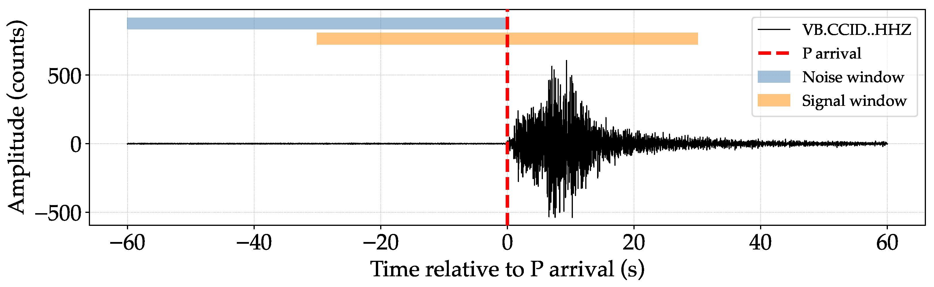
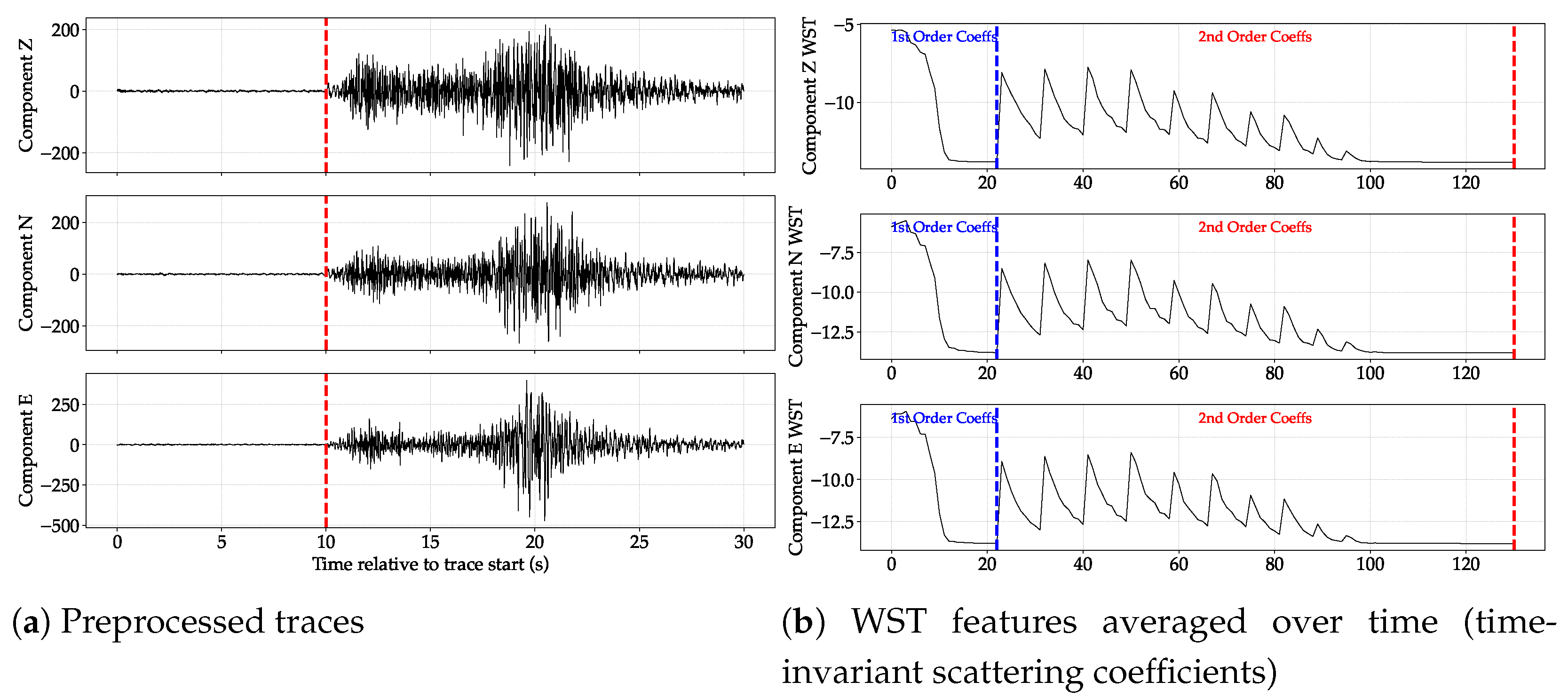
To illustrate the effect of the preprocessing stage, Figure 5 shows an example of a three-component windowed trace corresponding to the earthquake event vb2025ehdey of local magnitude 2.64 recorded at the Lucena del Cid Forest Observatory station (station code CCID). The raw traces are displayed exactly as recorded by the seismometers, while the preprocessed traces are obtained after applying the preprocessing steps described above. In the original traces, the signal amplitude is shown in counts, while in the preprocessed traces, the signal amplitude is shown on a normalized scale after performing the scaling operation.

4.2. Feature Extraction Using WST

In this step, the WST is computed for each component (Z, N, E) present in the traces using a 2-layer 1-D wavelet scattering network to obtain the first- and second-order scattering coefficients. For the scattering network definition, the number of wavelet filters per octave used was $Q_1=2$ and $Q_2=1$ for the first- and second-order filterbanks, respectively. The temporal invariance scale used was $T=2^{11}$. 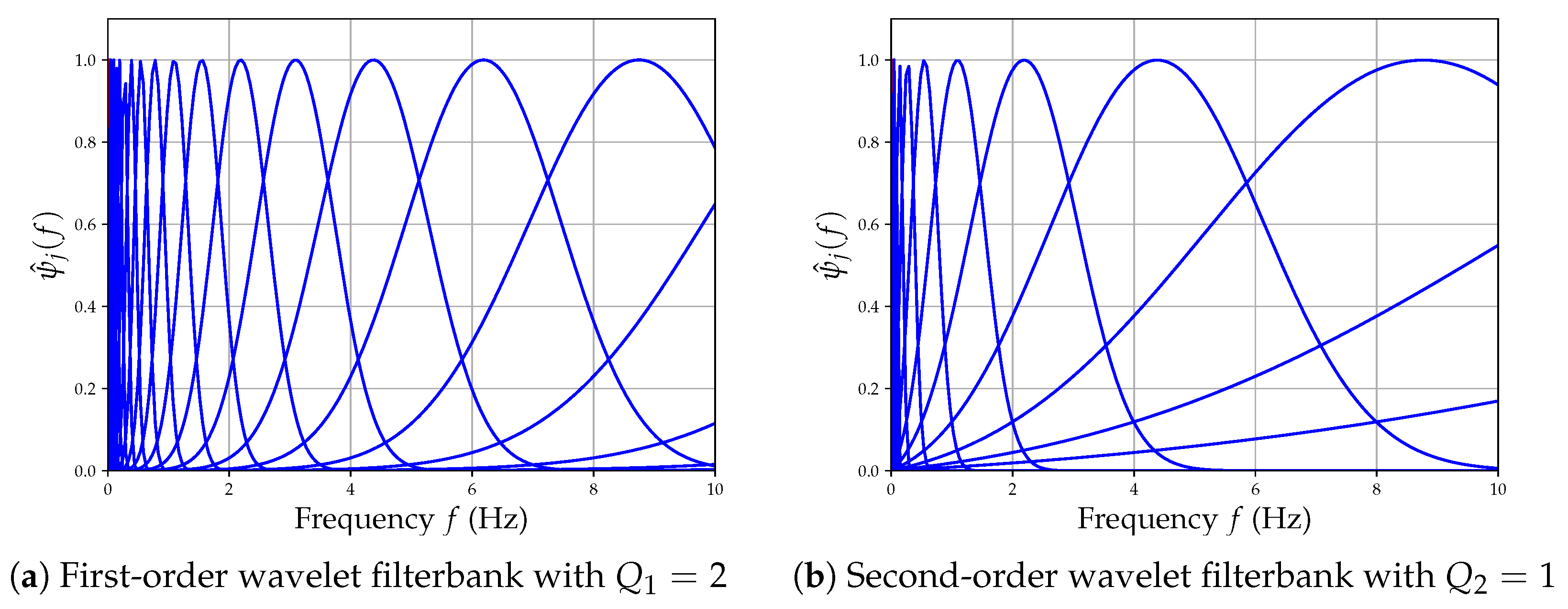Figure 6 shows the frequency response for the wavelet filterbanks used in each layer of the scattering network. Even though the wavelet filterbanks span the entire frequency range up to $f_s/2$ (50 Hz), in the plots only the interval $f\in [0,10 \mathrm{Hz}]$ in which most of the energy of the seismic events is concentrated is shown.

To eliminate the time dependence in the obtained WST matrix and convert it into a time-invariant representation, the logarithm of the absolute values of the coefficients is taken, and they are averaged over time. This yields the time-invariant scattering coefficients, which provide a sparser representation that may be easier to learn by machine learning classifiers to distinguish between events and noise representations. In this process, the zero-order coefficients are discarded, as they contain no discriminative information. For the scattering network defined with $J=11$ and $(Q_1,Q_2)=(2,1)$, 23 first-order and 108 s order time-invariant scattering coefficients (131 in total) are obtained per component.

Figure 7 shows an example of the time-invariant scattering coefficients computed for the 30-s window containing the recording from the CCID station of the earthquake event vb2025ehdey shown in Figure 5.

4.3. Dimension Reduction by PCA Analysis

The coefficients obtained for each component are concatenated into a single feature vector. Each signal window is thus represented as a high-dimensional feature vector containing the time-invariant scattering coefficients for each of the components in the signal window.

Due to the high dimensionality of the resulting coefficient vector (particularly due to the inclusion of second-order coefficients), a dimension reduction step is added using PCA. The component retention criterion is set at 95% of the explained variance, so that the number of principal components is automatically determined from the training data. This step serves a dual purpose: it eliminates the inherent multicollinearity among adjacent scattering coefficients and reduces the risk of overfitting the classifier. The PCA is performed exclusively on the training data, preventing any leakage of information from the test set into the model.

PCA on the training data feature vectors yielded a dimensionality reduction from 393 components to 31 principal components for 95% of explained variance, a substantial reduction of the original dimensionality that retains the majority of the information contained in the signal representation.

4.4. Feature Vector Classification by SVM

To classify the dimensionality-reduced feature vectors, an SVM classifier with a radial basis function (RBF) kernel was trained. The classifier’s hyperparameters are $C=10$ and $\gamma =1/(n_{features}·Var\left(features\right))$. The classifier produces a final label corresponding to the seismic signal window under analysis, indicating whether this window contains only noise or, conversely, contains a seismic event.

4.5. Implementation Details

Table 3. Configuration parameters of the event detection pipeline.

Parameter	Value
Window size	30 s
Filter	High-pass, $f_c=2$ Hz
Scaling interval	[$-1$; 1]
WST coefficient orders	1st and 2nd
$(Q_1,Q_2)$	(2, 1)
J	11
T	$2^{11}$
Variance retained by PCA	95
Number of feature dimensions after PCA	31
SVM-RBF C parameter	10
SVM-RBF $\gamma$ parameter	$1/(n_{features}·Var\left(features\right))$

summarizes the configuration parameters used for each of the pipeline stages:

All the data processing and tests were performed using Python 3.14.5. For the handling of data, the SeisBench v0.11.5 and ObsPy v1.5.0 packages were used [65,66]. As the original samples in the dataset were written in 60-s windows, a SeisBench random window generator was used to randomly select 30-s windows around the P arrival in the event samples of the dataset, ensuring that at least 15 s of post-P content was contained in every event window to avoid losing the information content of the event. This also ensured that for all training and testing samples, the event and noise content was not always located in the same intervals within the 30-s windows.

The 30-s window was not an arbitrary hyperparameter but a constrained choice driven by two factors. An inspection of the full SISCOVA catalog confirmed that the P-wave onset, S-wave arrival, and coda of every local event in the dataset are fully contained within a 30-s window given the source-station distances characteristic of the local network events. A shorter window would risk truncating the coda/S-wave portion of the more distant or emergent events in the catalog, degrading the completeness of the wavelet scattering representation for the events most likely to be misclassified. A longer window would add no additional signal content for any event in the dataset while increasing the input dimensionality processed by the WST.

In addition to this, 30 s is one of the de facto standard input lengths for earthquake detection/phase-picking architectures. Of the three deep learning architectures we used as comparison baselines in this paper, PhaseNet [32] and CRED [34] take 30-s seismograms sampled at 100 Hz as input. EQTransformer [33] is the exception as it operates on 60-s waveform windows, given its more complex architecture based on attention mechanisms and its orientation toward the processing of teleseismic events. Other lightweight architectures such as LightEQ [11], SeismicSense [47], ICAT-net [48] and LFTnet [50] also use 60-s inputs, which is a window size longer than the one needed to cover the seismic content of local events within the SISCOVA network.

For the implementation of the filtering and scaling operations, the functions available in the SciPy v1.17.1 and Scikit-learn v1.8.0 packages were used [67,68]. The WST coefficients were computed using the Kymatio v0.3.0 library [69]. The Scikit-learn v1.8.0 library was used in the implementation of the classifier pipeline, including dimensionality reduction with PCA and classification with SVM [70]. Besides this, the NumPy v2.4.4 and Matplotlib v3.10.8 packages were used respectively for general numerical and vector operations, and data visualization [71,72].

5. Results and Discussion

This section presents the results obtained from evaluating the proposed pipeline for seismic event detection using different experimental configurations. The objective is to quantify the impact of the training data quality on the classifier performance and to assess the limitations of the proposed approach. A direct comparison is then made with the classical detection method based on STA/LTA onset detection, which serves as the baseline for seismic monitoring. Finally, to compare the proposed detection pipeline within the current framework of seismic detection methods, three state-of-the-art deep learning models, PhaseNet [32], EQTransformer [33], and CRED [34], have been evaluated in a zero-shot transfer setting on the dataset used.

The experiments are structured into three different configurations of the train/test data for the pipeline proposed in this paper and one configuration for the other methods. The data configurations are based on data quality measured by the signal-to-noise ratio (SNR) of events.

Table 4. Evaluated experimental configurations.

Exp.	Training Data	Test Data	Method
E1	All data	All data	WST + PCA + SVM (this paper)
E2	Events with $\mathrm{SNR}\ge 6$ dB	All data	WST + PCA + SVM (this paper)
E3	Events with $\mathrm{SNR}\ge 6$ dB	Events with $\mathrm{SNR}\ge 6$ dB	WST + PCA + SVM (this paper)
E4	Events with $\mathrm{SNR}\ge 6$ dB	Events with $\mathrm{SNR}\ge 6$ dB	Recursive STA/LTA
E5	Events with $\mathrm{SNR}\ge 6$ dB	Events with $\mathrm{SNR}\ge 6$ dB	PhaseNet (original weights)
E6	Events with $\mathrm{SNR}\ge 6$ dB	Events with $\mathrm{SNR}\ge 6$ dB	EQTransformer (original weights)
E7	Events with $\mathrm{SNR}\ge 6$ dB	Events with $\mathrm{SNR}\ge 6$ dB	CRED (original weights)

illustrates the conditions used for each experiment conducted for every evaluated method.

The results obtained for each experiment are reported in terms of overall accuracy, precision, recall, and F1-score per class, and are supplemented with the corresponding confusion matrices. In each case, a discussion is provided.

5.1. Evaluation of the Proposed Method

Experiment E1 establishes the baseline performance of the proposed pipeline by using the entire set of available samples without applying any quality criteria to the training and test signals. The hyperparameter search for the classifier yielded a regularization parameter $C=100$ and a radial basis function (RBF) kernel with $\gamma =0.001$ as the optimal hyperparameters. The principal component analysis resulted in 34 components for 95% of explained variance.

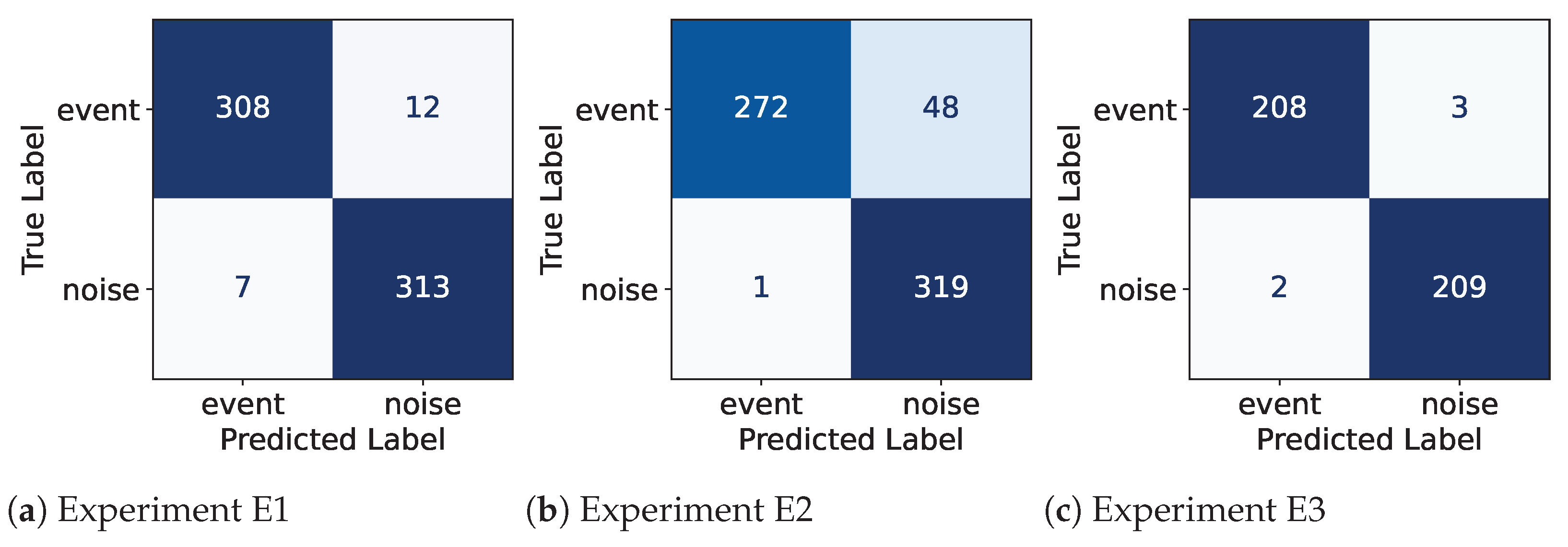
An overall accuracy of 97.03% and an average F1-score of 0.9703 are obtained for E1. Similar behavior is observed in terms of precision and recall for both classes. However, an in-depth analysis of the test samples corresponding to seismic events that the pipeline misclassifies as noise reveals that the vast majority of these signals correspond to seismic events with a very low signal-to-noise ratio. This suggests that the presence of samples in which the seismic event energy is hardly distinguishable from the noise in the training subset (probably due to the large distance between the event and the station corresponding to the record) negatively affects the model’s ability to reject noise. This is because these samples, treated during training as seismic events, exhibit features similar to those of noise and adversely influence the classifier’s learning process during its training, causing a moderate increase in the false positive rate.

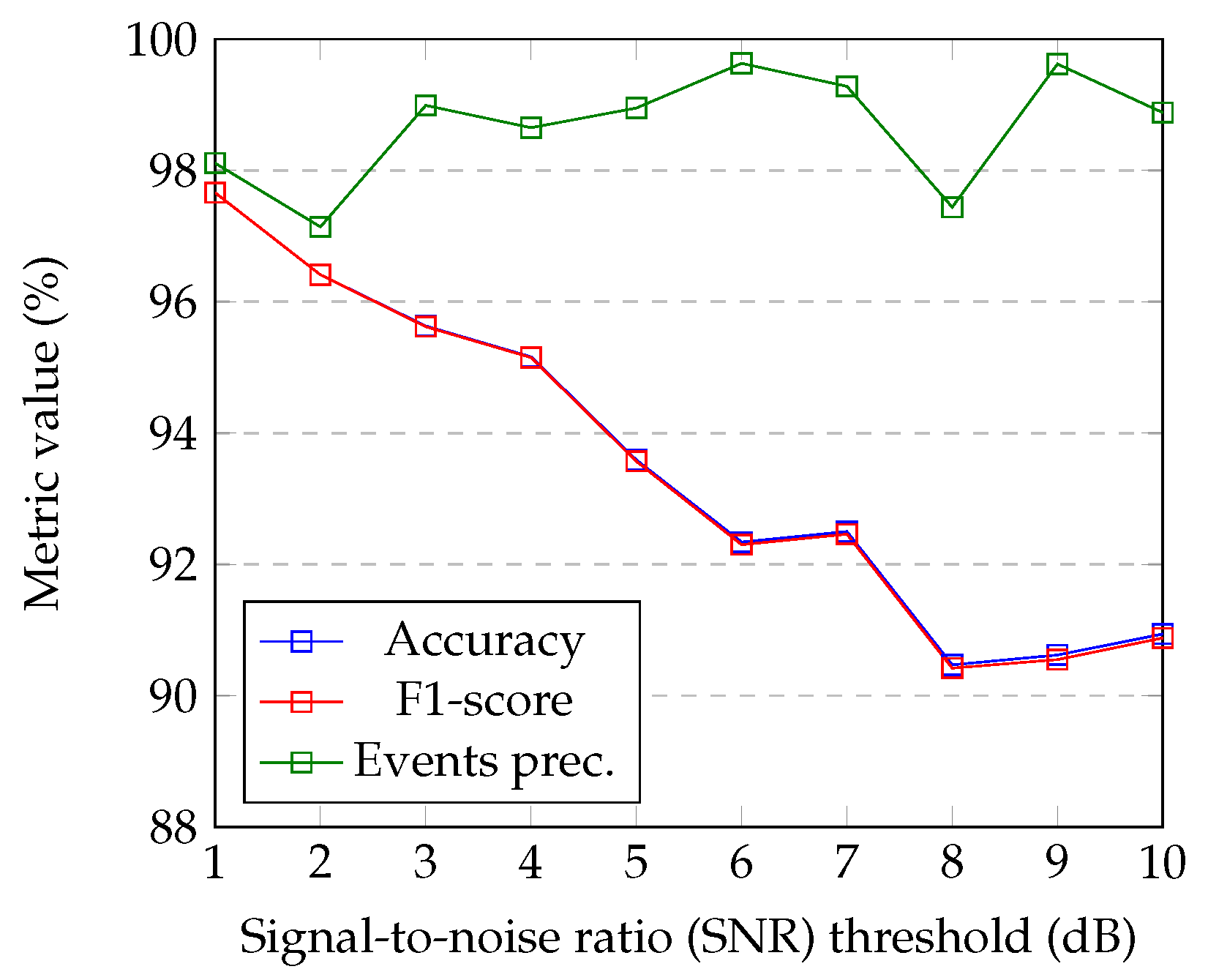
This suggests the convenience of establishing a data quality criterion for the training data based on event SNR. To establish the data quality baseline that maximizes the classifier’s detection performance, the pipeline was evaluated on the entire test data subset after restricting the training data to different minimum SNR values in the interval [1, 10] dB. Figure 8 shows the results obtained in terms of overall accuracy, F1-score, and event-class precision for each considered SNR threshold.

As can be seen in Figure 8, the overall accuracy and F1-score decrease as the minimum SNR required for the training data increases. This occurs because the classifier’s ability to correctly identify low-SNR events gets compromised as the training data quality is restricted to higher SNR events. However, event precision increases for most cases in relation to experiment E1, indicating a lower false positive rate. It can be seen that the SNR threshold that achieves the best compromise between accuracy/F1-score and event precision is $\mathrm{SNR}=6$ dB.

Experiment E2 evaluates the effect of restricting the training set to samples with $\mathrm{SNR}\ge 6$ dB, while keeping the test set unchanged. This configuration simulates the scenario of greatest practical interest: a model trained on clean records that must operate on signals of arbitrary quality, including noisy or low-SNR records that the model will inevitably encounter in the real-world scenario. The comparison with E1 allows us to isolate the effect of filtering the training data to high-quality samples on the false positive rate. The search for classifier hyperparameters performed via grid search yielded, in this case, a regularization parameter $C=10$ and a radial basis function (RBF) kernel with $\gamma =1/(n_{features}·Var\left(features\right))$ as the optimal hyperparameters. Principal component analysis resulted in 31 components for 95% of explained variance in the original features. An overall accuracy of 92.34% and an average F1-score of 0.9230 are obtained. However, in this case, the precision for the event class, which is 0.9963, is much higher than for the noise class, which is 0.8692. A thorough analysis of the misclassified signals reveals that those signals with low SNR, where the seismic event is not clearly distinguishable from noise, are classified as noise. However, there are fewer noise signals misclassified as events compared to the previous experiment, reducing the false positive rate. By using cleaner signals for training, the model learns to better identify the features that define a seismic event.

This result demonstrates that the presence of signals with very low SNR in the training set negatively affects the detection model’s ability to reject noise signals that may resemble seismic events received at stations with very low intensity. However, at the same time, the model becomes more demanding regarding the SNR an event must have to be detected. Nevertheless, this allows for the establishment of quantitative criteria regarding the conditions under which an event must be recorded at the stations for it to be detected by the model. To validate this hypothesis, experiment E3 was conducted.

Experiment E3 applies data selection based on $\mathrm{SNR}\ge 6$ dB to both the training and test data subsets, thereby evaluating the pipeline’s performance under controlled conditions where both partitions contain only high-quality records. The noise class was subsampled according to the number of events that met the SNR $\ge 6$ dB criterion to keep the class balance. Although this scenario is not directly representative of real-world operational conditions, it provides an estimate of the maximum performance achievable by the pipeline on high-quality data, serving as an upper bound. The comparison between E2 and E3 quantifies the performance degradation introduced by low-SNR samples in the test set. For this experiment, the selection of hyperparameters yielded the same results as experiment E2, as the same training data was used.

The overall accuracy obtained for E3 is 98.82%. For high-quality data (events with an SNR equal to or greater than 6 dB), the proposed pipeline detects seismic events with great effectiveness while maintaining a low false positive rate. This confirms that the performance degradation observed in experiment E2 stems from the presence of very low-SNR signals in the test set.

Table 5. Classification metrics for experiments E1, E2 and E3.

Experiment	Class	Precision	Recall	F1-Score	Support
E1	Noise	0.9631	0.9781	0.9705	320
	Event	0.9778	0.9625	0.9701	320
	Overall	0.9704	0.9703	0.9703	640
E2	Noise	0.8692	0.9969	0.9287	320
	Event	0.9963	0.8500	0.9174	320
	Overall	0.9328	0.9234	0.9230	640
E3	Noise	0.9858	0.9905	0.9882	211
	Event	0.9905	0.9858	0.9881	211
	Overall	0.9882	0.9882	0.9882	422

shows the detailed metrics for the three experiments conducted on the three different data configurations.

The confusion matrices for the test data in every experiment are shown in Figure 9.

5.1.1. Hyperparameter Optimization

For the scattering network definition, a grid search was performed on the training partition to find the optimal values for the temporal invariance scale T and the number of wavelet filters per octave $Q_1$ and $Q_2$ for the first- and second-order filterbanks, respectively. The values of T were selected from the range $[2^8,2^{11}]$, while the values of $Q_1$ and $Q_2$ were selected from the ranges $[1,8]$ and $[1,4]$, respectively. In the selection of the values for these parameters, priority was given to those that maximized the event class precision without compromising the F1-Score. The tests for this hyperparameter optimization process were performed using the data configuration of experiment E2, considering its more realistic representation of the real-world scenario.

A sequential search strategy was adopted, exploiting the structural role of T as the coarsest scattering network hyperparameter, because it fixes the temporal invariance scale, within which $Q_1$ and $Q_2$ subsequently determine filterbank density. The search proceeded in three stages. First, with $Q_1=Q_2=1$ fixed, T was swept over the range $[2^8,2^{11}]$, and the value maximizing the mean cross-validated F1-score and event precision was retained. To verify that this marginal criterion did not overlook a more favorable joint configuration, the second stage (the $Q_1$ sweep over $[1,8]$) was evaluated both at the T value of highest marginal F1-score ($T=2^9$) and at $T=2^{11}$, since this value corresponds to the largest temporal invariance scale in the range under consideration, which allows for a higher degree of invariance to temporal shifts. Higher values of T were not supported by the scattering network definition, considering the constraints imposed by the temporal support of the input signals and the number of wavelet filters per octave in the filterbank definition. Under this joint evaluation, $T=2^{11}$ combined with $Q_1=2$ achieved event precision superior to any configuration obtained at $T=2^9$, at a marginal F1-score cost of under one percentage point relative to the highest-scoring configuration overall. $T=2^{11}$ and $Q_1=2$ were retained on this basis, and $Q_2$ was subsequently swept over $[1,4]$ with T and $Q_1$ fixed.

Table 6. Sequential hyperparameter search results for the WST configuration (T, $Q_1$, $Q_2$). Bold indicates the selected value at each stage.

Stage	Parameter	F1-Score	Event Precision
T sweep ($Q_1=1,Q_2=1$)	$T=2^8$	0.8962	0.9739
	$T=2^9$	0.9231	0.9927
	$T=2^{10}$	0.9183	0.9926
	$T=2^{11}$	0.9184	0.9855
$Q_1$ sweep ($T=2^9,Q_2=1$)	$Q_1=1$	0.9231	0.9927
	$Q_1=2$	0.9326	0.9894
	$Q_1=3$	0.9373	0.9895
	$Q_1=4$	0.9294	0.9928
$Q_1$ sweep ($T=2^{11},Q_2=1$)	$Q_1=1$	0.9184	0.9855
	$Q_1=2$	0.9234	0.9963
	$Q_1=3$	0.9310	0.9894
	$Q_1=4$	0.9183	0.9963
$Q_2$ sweep ($T=2^{11},Q_1=2$)	$Q_2=1$	0.9234	0.9963
	$Q_2=2$	0.9167	0.9963

reports the results obtained on the test data fold for a representative subset of the evaluated configurations; higher-order values of $Q_1$ and $Q_2$ produced no further gain in either metric and are omitted for simplicity. The final selected configuration, $T=2^{11}$, $Q_1=2$ and $Q_2=1$, is highlighted in bold. In general, the pipeline did not experience a substantial performance sensitivity to the hyperparameter selection for the WST computation, so lower values of $Q_1$ and $Q_2$ are considered more appropriate to keep the computing cost as low as possible.

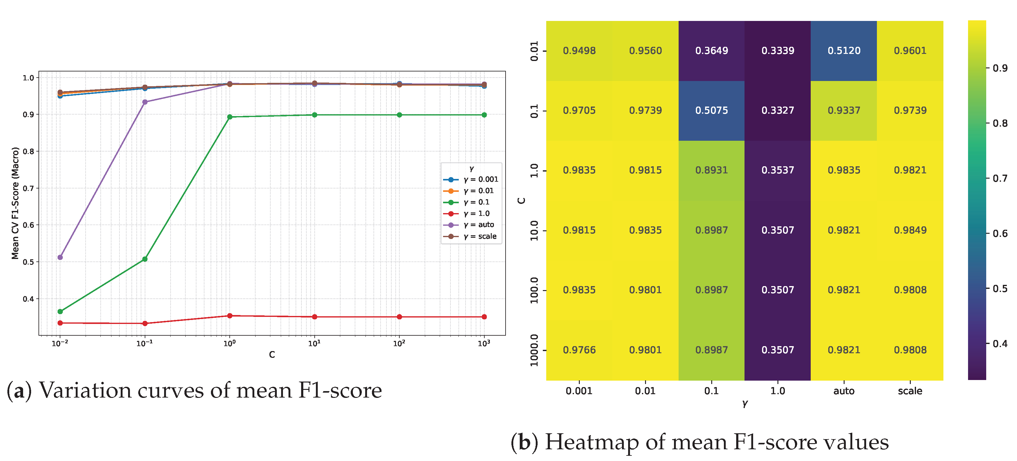
For all experiments, the values of the hyperparameters C and $\gamma$ for the SVM classifier with RBF kernel were determined through an exhaustive grid search with stratified cross-validation in the search space $C\in \{0.01,0.1,1,10,100,1000\}$ and $\gamma \in \{$0.001,0.01,0.1,1.0$,1/n_{features}\left(auto\right),1/(n_{features}·Var\left(features\right))\left(scale\right)\}$, optimizing the mean F1-score over the training fold. Stratification preserves the class proportions in each batch of data used in the cross-validation process. Figure 10 shows the variation curves and heatmap of the mean F1-score values over C and $\gamma$ for the SVM classifier with RBF kernel using the selected WST hyperparameters.

The highest mean F1-score is obtained for $C=10$ and $\gamma =1/(n_{\mathrm{features}}·\mathrm{Var}\left(\mathrm{features}\right))$ (scale).

5.1.2. Ablation Tests

To isolate the individual and joint contributions of each preprocessing stage in the proposed detection pipeline and demonstrate its necessity, a full factorial ablation study was performed over three binary design factors: the number of seismic components used as input (three-component ZNE vs. vertical-only Z), the scattering order of the WST (first-order vs. second-order), and the use of raw scattering coefficients vs. PCA-reduced coefficients as SVM input. This yields a factorial design with eight configurations. For the ablation tests, the data configuration of experiment E2 was also used. The classifier is fixed as an RBF-SVM, and its hyperparameters are retuned for each test using a grid search on the training fold. The PCA components were selected to explain 95% of the variance, and for the WST, the number of wavelet filters per octave was set to $Q_1=2$ and $Q_2=1$ for the first- and second-order filterbanks, respectively, for all cases.

Table 7. Full factorial ablation test results.

Components	WST Order	Features	Accuracy	F1-Score	Event Precision
ZNE	2nd-order	PCA-reduced	0.9234	0.9230	0.9963
ZNE	2nd-order	Raw	0.9234	0.9231	0.9927
ZNE	1st-order	PCA-reduced	0.8812	0.8806	0.9453
ZNE	1st-order	Raw	0.8953	0.8946	0.9738
Z	2nd-order	PCA-reduced	0.9000	0.8994	0.9706
Z	2nd-order	Raw	0.9062	0.9057	0.9815
Z	1st-order	PCA-reduced	0.8438	0.8425	0.9198
Z	1st-order	Raw	0.8609	0.8596	0.9494

summarizes the results for each test configuration in terms of overall accuracy, F1-score, and event precision.

The ablation test results establish a clear ordering of factor importance among the three design axes considered. Scattering order exerts the largest main effect, with second-order configurations reaching a mean F1-score up to 5% higher than first-order configurations. The choice of input components produces a comparable but secondary effect, with three-component (ZNE) configurations outperforming vertical-only (Z) configurations by around 2.5% in mean F1-score. This is consistent with horizontal-component energy carrying discriminative information that the vertical channel alone does not capture. Finally, the raw-versus-PCA-reduced axis shows the smallest main effect among the three factors considered. Raw scattering coefficients yield only a marginally higher mean F1-score than their 95%-variance PCA-reduced counterparts, confirming that the dimensionality reduction achieved by PCA does not come at a meaningful cost in discriminative performance. This near-equivalence indicates that PCA’s role in this pipeline is to deliver dimensionality and compute-cost reduction while preserving the accuracy of the full-dimensional representation, supporting its inclusion in the final architecture as a favorable trade-off.

The full-pipeline configuration (ZNE, 2nd-order WST and PCA-reduced features) attains the highest event precision among all eight configurations while matching its raw-feature counterpart’s accuracy and F1-score to within 0.01%, being the best of all configurations.

5.2. Comparison with STA/LTA Method

For comparison, a classical detector based on the traditional recursive STA/LTA algorithm (Short-Term Average/Long-Term Average) has been implemented [15]. This method calculates for each sample the ratio between the average of the signal in a short, transient-sensitive window and the average amplitude in a long window, declaring an event detected when this ratio exceeds a predefined threshold. Detection has been applied to the vertical Z component of the same samples from the test subset used in E3, ensuring that the signals met the criterion $\mathrm{SNR}\ge 6$ dB to directly compare this approach with the results obtained for the proposed pipeline. The threshold was determined by evaluating the detector on the training data split over thresholds $\tau \in [1.00,10.00]$ in increments of 0.01 and selecting the value that maximized a selected metric. Two metrics were used as targets for optimization: the overall F1-score and the precision for the event class (targeting the lowest possible false positive rate).

The parameters of the STA/LTA detector used were:

• Short window length: $t_{\mathrm{STA}}=0.5$ s,
• Long window length: $t_{\mathrm{LTA}}=4.0$ s,

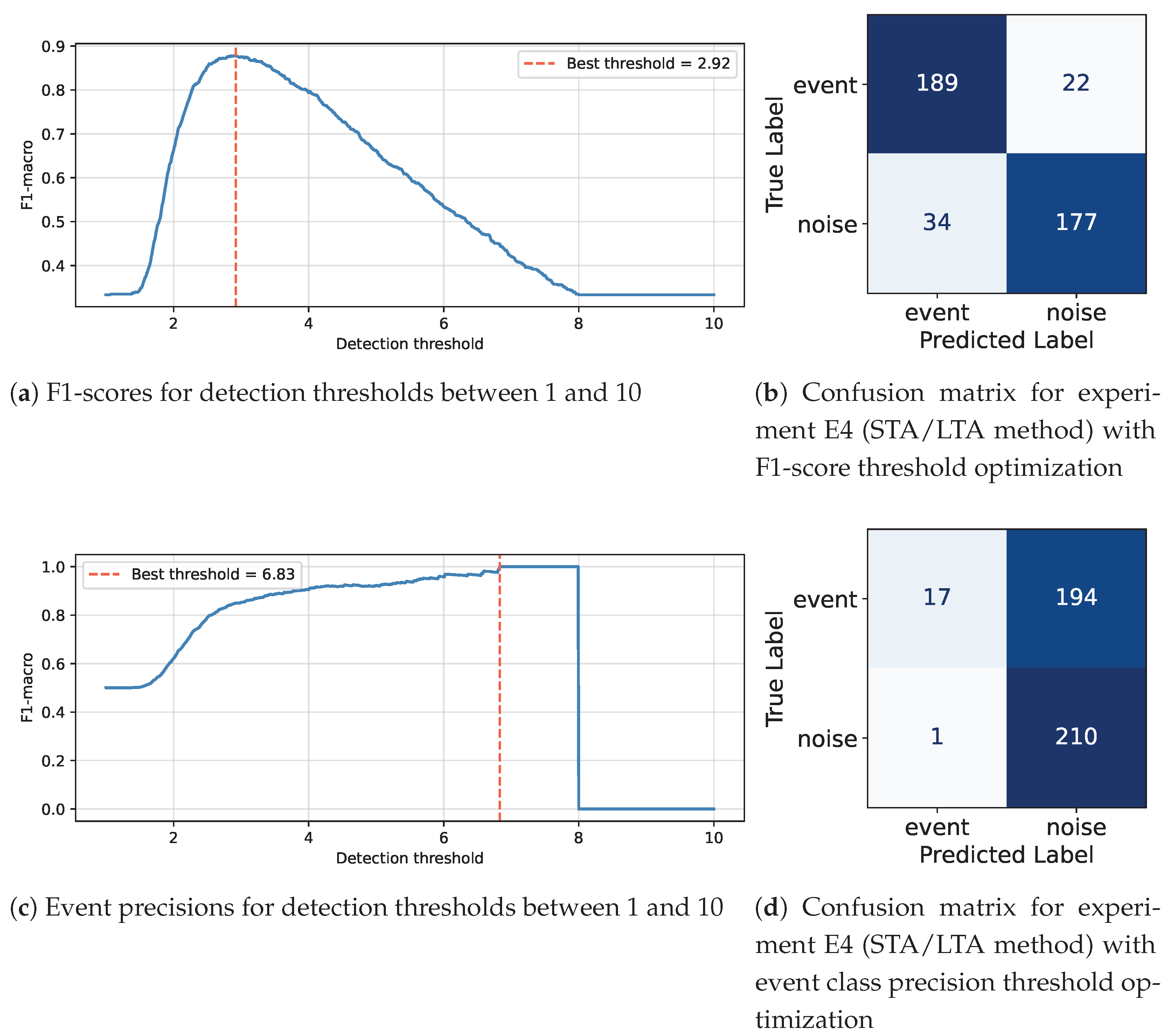
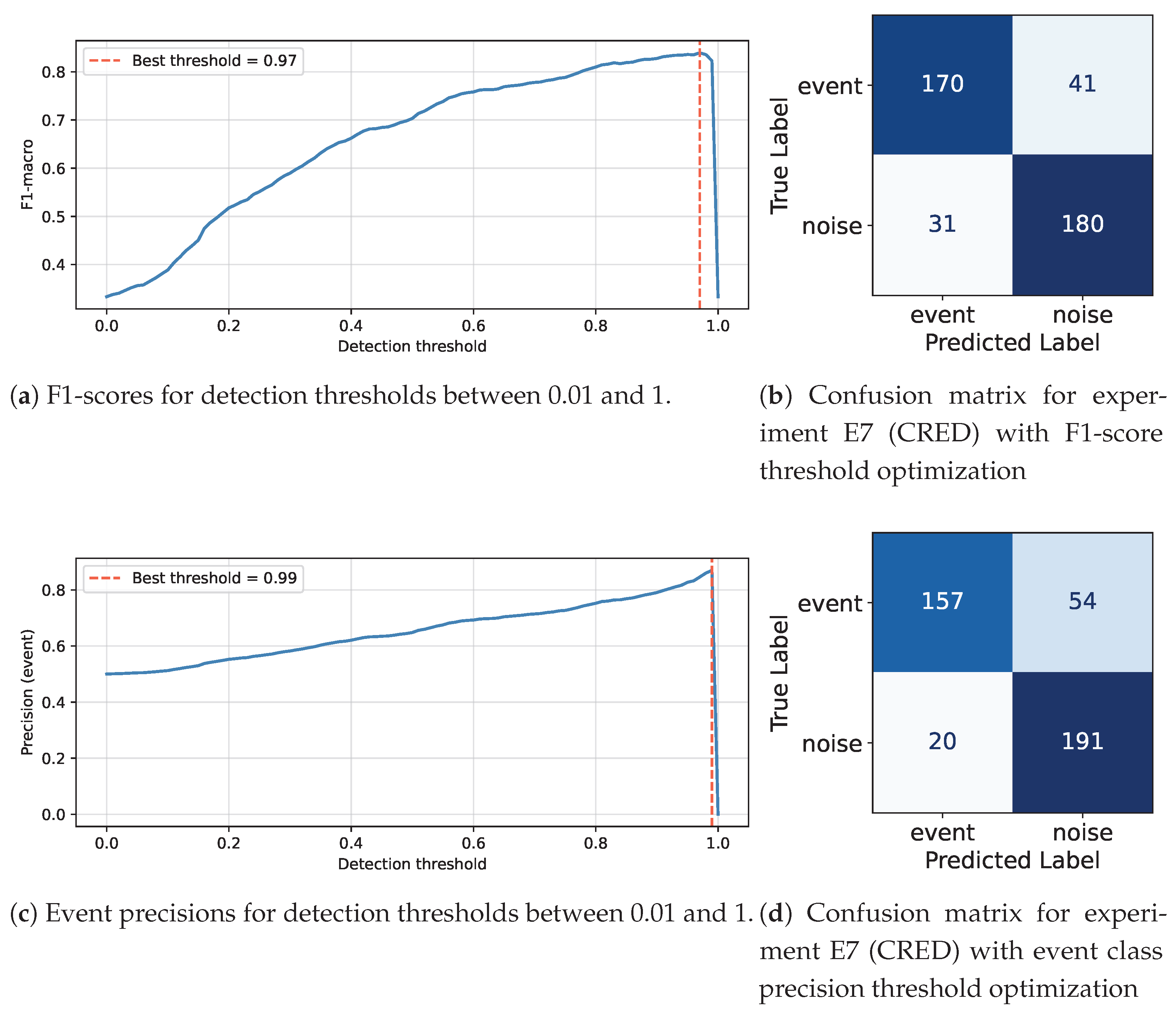
Figure 11 shows the results of the evaluation of the STA/LTA detector. On the left, the threshold sweep optimization results using the F1-scores and the event class precisions as target metrics for optimization of the train data split are presented. On the right, the confusion matrices obtained on the test data for the best thresholds are shown.

Table 8. Classification metrics for STA/LTA detector with thresholds ${\tau }_{\mathrm{STA}/\mathrm{LTA}}=2.92$ for F1-score optimization and ${\tau }_{\mathrm{STA}/\mathrm{LTA}}=6.55$ for event class precision optimization.

Threshold	Class	Precision	Recall	F1-Score	Support
$\tau =2.92$	Noise	0.8894	0.8389	0.8634	211
	Event	0.8475	0.8957	0.8710	211
	Overall	0.8685	0.8673	0.8672	422
$\tau =6.83$	Noise	0.5198	0.9953	0.6829	211
	Event	0.9444	0.0806	0.1485	211
	Overall	0.7321	0.5379	0.4157	422

summarizes the evaluation metrics on the test data split for the best thresholds obtained in each case.

The overall accuracy obtained for this experiment is 86.73% for ${\tau }_{\mathrm{STA}/\mathrm{LTA}}=2.92$ (F1-score optimized threshold) and 53.79% for ${\tau }_{\mathrm{STA}/\mathrm{LTA}}=6.83$ (event class precision optimized threshold). The confusion matrix for ${\tau }_{\mathrm{STA}/\mathrm{LTA}}=2.92$ reveals a considerable number of false positives, which seriously compromise the practical utility of using this method as a detection algorithm in a real-time seismic monitoring system. On the other hand, optimizing the threshold for the event class precision makes the detector completely biased towards the noise class. This highlights the robustness of the proposed approach compared to the traditional STA/LTA detection method.

5.3. Comparison with Deep Learning Techniques

The deep learning models of PhaseNet, EQTransformer, and CRED were loaded with their publicly released original weights, trained on large-scale global catalogs, and applied directly to the same test split of data with SNR $\ge 6$ dB. For these experiments, the SeisBench framework was used, and the models used are the ones available in it [65].

Two temporal window configurations were prepared to match the input requirements of each architecture. PhaseNet and CRED accept fixed-length inputs of 3001 and 3000 samples at 100 samples per second (30 s), respectively, while EQTransformer requires 6000-sample (60 s) input windows. Accordingly, two instances of the dataset were constructed from the source dataset using the SeisBench random window generator: one with a 30 s window size, used for PhaseNet and CRED, and a second with a 60 s window size, used exclusively for EQTransformer. In both cases, waveforms were loaded with three-component Z, N, E ordering and subjected to the same preprocessing operations applied in the WST-based pipeline.

The PhaseNet, EQTransformer, and CRED models are sequence-to-sequence models that generate output probability heads of the same length as the input signals, containing probability values associated with the temporal evolution of the samples for the presence of P or S phases or simply the presence of events. EQTransformer and CRED both have a dedicated output head for detection, whereas PhaseNet has only P- and S-phase output heads, as it is explicitly designed as a phase picker.

Because of this behavioral difference from the pipeline proposed in this paper, a simple event detection strategy was implemented that leverages these probabilistic output heads. A window was considered to be a seismic event if the maximum absolute value in the corresponding output heads exceeded a defined threshold; otherwise, the window was classified as noise. For PhaseNet, this maximum absolute value was determined from the P and S phase probability heads (consistent with the common usage of phase pickers as event detectors), whereas in the cases of EQTransformer and CRED, the detection output heads were used. For all cases, the threshold was determined by evaluating the models on the training data split over thresholds $\tau \in [0.01,1.00]$ in increments of 0.01 and selecting the value that maximized a selected metric. Just as for the STA/LTA detector, the two metrics used as targets for optimization were the overall F1-score and the precision for the event class (targeting the lowest possible false positive rate).

5.3.1. Zero-Shot Evaluation of PhaseNet

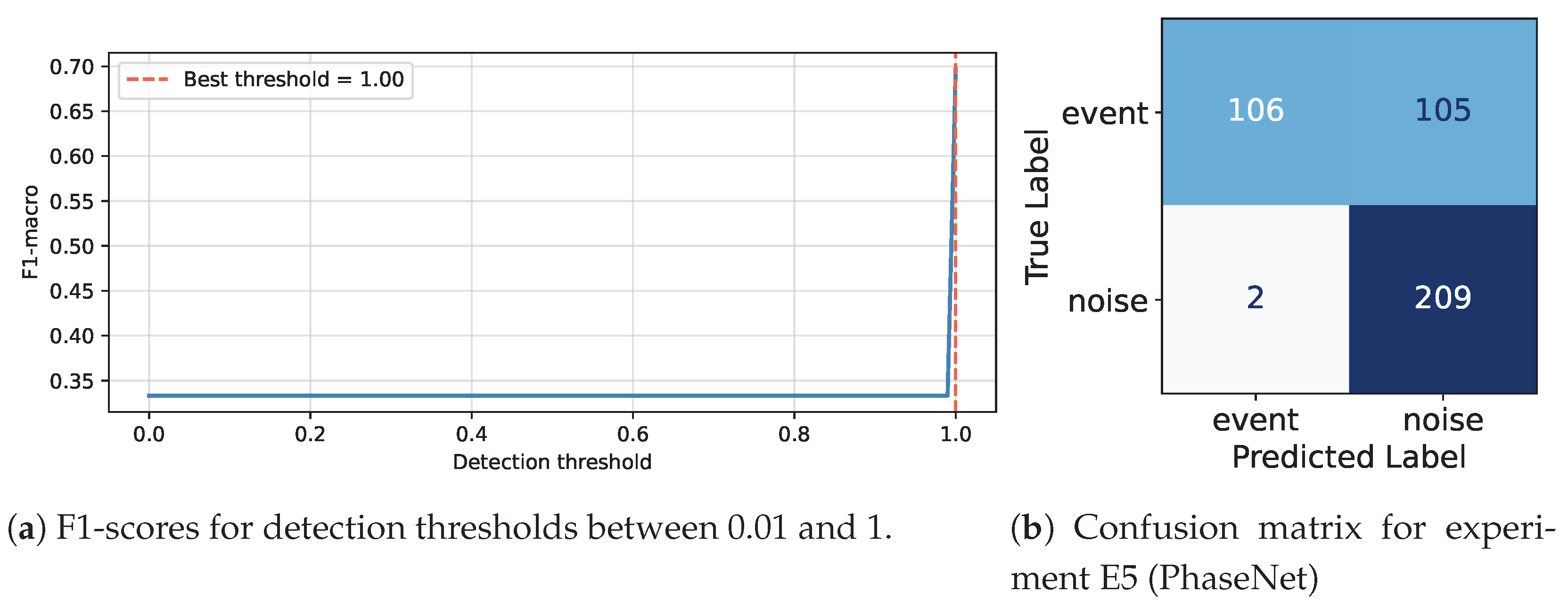
Figure 12 shows the results of the evaluation of the PhaseNet model. On the left, the threshold sweep optimization results using the F1-scores and the event class precisions as target metrics for optimization of the train data split are presented (the same results were obtained for both metrics). On the right, the confusion matrix obtained on the test data for the best threshold is shown.

Table 9. Classification metrics on the test data split for PhaseNet with threshold ${\tau }_{\mathrm{PhaseNet}}=1.00$.

Class	Precision	Recall	F1-Score	Support
Noise	0.6656	0.9905	0.7962	211
Event	0.9815	0.5024	0.6646	211
Overall	0.8235	0.7464	0.7304	422

summarizes the evaluation metrics on the test data split for the best threshold.

As can be seen from the results, an overall accuracy of 74.64% was obtained for PhaseNet on the test data, with no change being made by the target metric selection in the threshold optimization.

5.3.2. Zero-Shot Evaluation of EQTransformer

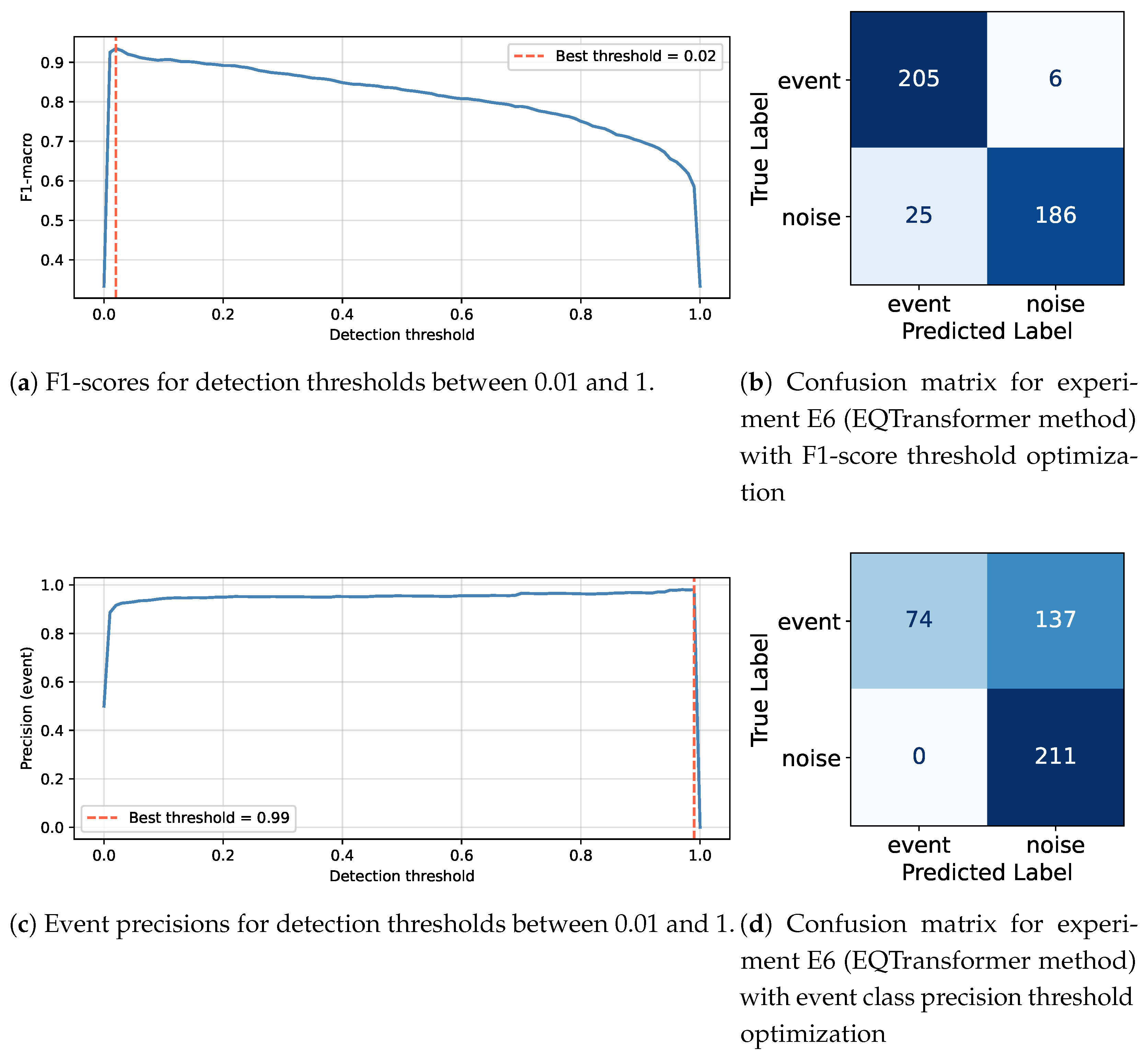
Figure 13 shows the results of the evaluation of the EQTransformer model. The figure is structured in the same way as Figure 12.

Table 10. Classification metrics on the test data split for EQTransformer with thresholds ${\tau }_{\mathrm{EQTransformer}}=0.02$ for F1-score optimization and ${\tau }_{\mathrm{EQTransformer}}=0.95$ for event class precision optimization.

Threshold	Class	Precision	Recall	F1-Score	Support
$\tau =0.02$	Noise	0.8913	0.9716	0.9297	211
	Event	0.9688	0.8815	0.9231	211
	Overall	0.9300	0.9265	0.9264	422
$\tau =0.99$	Noise	0.6063	1.0000	0.7549	211
	Event	1.0000	0.3507	0.5193	211
	Overall	0.8032	0.6754	0.6371	422

summarizes the evaluation metrics on the test data split for the best thresholds optimized for each target metric.

The results show an overall accuracy of 92.65% for the F1-score optimized threshold and 67.54% for the event precision optimized threshold. For the F1-score optimized threshold, the model achieves higher overall metrics, whereas for the event class precision optimized threshold, the model achieves a null false positive rate at the cost of a much lower capacity to detect true events.

5.3.3. Zero-Shot Evaluation of CRED

Figure 14 shows the results of the evaluation of the CRED model. The figure follows the same structure as Figure 12 and Figure 13.

Table 11. Classification metrics on the test data split for CRED with thresholds ${\tau }_{\mathrm{CRED}}=0.97$ for F1-score optimization and ${\tau }_{\mathrm{CRED}}=0.99$ for event class precision optimization.

Threshold	Class	Precision	Recall	F1-Score	Support
$\tau =0.97$	Noise	0.8145	0.8531	0.8333	211
	Event	0.8458	0.8057	0.8252	211
	Overall	0.8301	0.8294	0.8293	422
$\tau =0.99$	Noise	0.7796	0.9052	0.8377	211
	Event	0.8870	0.7441	0.8093	211
	Overall	0.8333	0.8246	0.8235	422

summarizes the evaluation metrics on the test data split for the best thresholds optimized for each target metric.

The results show an overall accuracy of 82.94% for the F1-score optimized threshold and 82.46% for the event class precision optimized threshold. In this case, contrary to EQTransformer, the performance was similar for both optimized thresholds, as the thresholds are very close, so the target metric made no significant impact on the overall detection performance.

5.4. Discussion

Table 12. Summary of overall detection performance for all evaluated methods on the SNR ≥ 6 dB data quality test subset with support of 422 samples (211 events and 211 noise samples).

Method	Accuracy	F1-Score	Event Prec.
WST+PCA+SVM (This paper)	0.9882	0.9882	0.9905
STA/LTA (Traditional approach [15], F1-opt)	0.8673	0.8672	0.8475
STA/LTA (Traditional approach [15], prec.-opt)	0.5379	0.4157	0.9444
PhaseNet (DL approach [32], F1 and prec.-opt)	0.7464	0.7304	0.9815
EQTransformer (DL approach [33], F1-opt.)	0.9265	0.9264	0.9688
EQTransformer (DL approach [33], prec.-opt.)	0.6754	0.6371	1.0000
CRED (DL approach [34], F1-opt.)	0.8294	0.8293	0.8458
CRED (DL approach [34], prec.-opt.)	0.8246	0.8235	0.8870

summarizes the detection performance for all evaluated methods on the SNR ≥ 6 dB data quality test subset. The comparative results situate the proposed pipeline within the current landscape of seismic event detection methods, evaluated under known conditions (SNR ≥ 6 dB) for all approaches. The proposed pipeline clearly outperforms both the classical STA/LTA baseline and all three pretrained deep learning models evaluated in a zero-shot transfer setting.

Among the reference methods evaluated, EQTransformer under F1-optimized thresholding achieves the closest performance to the proposed pipeline (accuracy and F1-score above 0.92), but its precision for the event class remains below that of the proposed approach, and its event precision-optimized configuration illustrates a steep trade-off: a perfect event precision is attainable only at the cost of a substantial drop in overall accuracy and F1-score (to below 0.70). This sensitivity to the threshold selection criterion is itself a practical limitation, since it implies that the operating point cannot be fixed reliably without access to representative local data for calibration.

PhaseNet shows the weakest overall accuracy and F1-score among all methods, despite its high event precision. This indicates that the model performs as a conservative detector that rarely raises false alarms but at the cost of missing a substantial fraction of true events. CRED occupies an intermediate position, with accuracy and F1-score around 0.82–0.83 and event precision in the 0.84–0.89 range, relatively stable across both threshold optimization criteria, but also below that achieved by the proposed method.

These results indicate that the proposed pipeline, achieving uniformly high performance across all three axes, performs consistently better than all the evaluated reference methods for the data acquired in the local SISCOVA network. This supports its suitability as a robust alternative for tailored seismic event detection in local seismic networks in which the amount of available data is limited. However, it must be noted that the performance gap observed for the pretrained deep learning models, which constitute the current reference in the literature for automatic event detection and phase picking, likely reflects a domain-shift effect inherent to zero-shot transfer rather than an intrinsic architectural limitation. It has already been demonstrated in other works that the generalization capabilities of these models may be compromised when applied to specific regions [36,37]. Moreover, the performance of these models can be significantly improved through fine-tuning on local data, which constitutes a potential direction of future work. Independently of this, the proposed method constitutes a much more computationally efficient alternative for embedded, low-power deployment in edge devices than the deep learning models, which are computationally expensive and require great amounts of memory to store their parameters. Although a full hardware benchmarking study is beyond the scope of this work, the architectural properties of the pipeline support this motivation qualitatively. Deployment on embedded hardware will require implementation of the Kymatio WST filter bank and a fixed-point SVM inference kernel; the feasibility and performance of this deployment constitute ongoing work and will be the subject of future studies.

5.5. Performance of the Proposed Method on Continuous Data

For the validation of the proposed method trained with data of SNR ≥ 6 dB as in experiments E2 and E3, we performed a qualitative assessment of its behavior on continuous, unsegmented, realistic recordings from the Lucena del Cid Forest Observatory station (CCID) and the Font Roja Sanctuary station (AFON) in the SISCOVA seismic network. The CCID station was selected because, being located in a 9-m borehole, it records fewer vibrations caused by anthropogenic surface activity than the other stations in the network. This simplifies evaluation of the detection pipeline, making it easier to check the events detected in the recordings against the register of known events from that day. AFON, by contrast, is located in a shallow seismic trench closer to the surface and records a considerable amount of anthropogenic activity, allowing generalization to be verified under strong anthropogenic noise. This analysis complements the quantitative evaluation performed in experiments E1-E3, where the models were evaluated on curated windows of data.

The daily recordings of the selected stations were read from their source .mseed files into continuous streams using the ObsPy framework in a Python script designed for this purpose. The continuous waveform streams were segmented into overlapping 30-s windows with a 10-s step between consecutive windows. Then, the WST+PCA+SVM pipeline was applied to every window to obtain a binary Event/Noise label. This operation was performed in a sequential loop that rejected the windows classified as noise and displayed the waveform and details of the windows classified as events. All the windows whose start times were separated by 20 s or less (twice the step size used) were grouped together to form window clusters, where each cluster of windows is considered to correspond to a seismic event (or several, depending on how close the seismic events occurred in time). Finally, an expert (human) review was performed to compare the clusters obtained against the records of known events to assess the correspondence with the known events from that day. The daily records analyzed were selected from two specific days (24 March 2024 and 6 September 2024) according to the representativeness of their recorded seismic activity.

5.5.1. Analysis of the 24 March 2024 Record

The events registered on 24 March 2024 present a low geographical dispersion, as they are clustered near $38.6^{\circ }$ N, $-0.{55}^{\circ }$ E. The records include 13 confirmed and 3 suspected local earthquake events with magnitudes between 1.38 and 3.28, and a known earthquake occurred outside of the network of interest area.

Table 13. Details of seismic events recorded on 24 March 2024 and picked by the Lucena del Cid Forest Observatory (CCID) and the Font Roja Sanctuary (AFON) stations.

No.	Event ID	Origin Time	Type	Certainty	Mag.	Picked by
1	vb2024fwhgr	07:54:31	-	suspected	-	AFON
2	vb2024fwtqy	14:10:11	EQ	known	1.90	CCID, AFON
3	vb2024fwwee	15:26:11	EQ	suspected	1.48	AFON
4	vb2024fwwik	15:31:07	EQ	suspected	1.38	AFON
5	vb2024fwxkr	16:04:05	EQ	known	2.72	CCID, AFON
6	vb2024fwxoh	16:08:18	EQ	known	3.00	CCID, AFON
7	vb2024fwyez	16:27:46	EQ	known	3.28	CCID, AFON
8	vb2024fwyga	16:28:58	EQ	known	2.48	CCID, AFON
9	vb2024fwyrj	16:42:12	EQ	known	1.5	AFON
10	vb2024fwyrt	16:42:39	EQ	known	1.73	CCID, AFON
11	vb2024fxatf	17:44:58	EQ	known	2.29	CCID, AFON
12	vb2024fxbxy	18:20:46	EQ	known	1.66	AFON
13	vb2024fxcbg	18:24:38	EQ	out of net. interest	2.41	CCID
14	vb2024fxcsm	18:44:42	EQ	known	1.41	AFON
15	vb2024fxisf	21:46:14	EQ	known	1.94	CCID, AFON
16	vb2024fxitj	21:47:37	EQ	known	1.62	AFON
17	vb2024fxiyc	21:53:07	EQ	known	1.45	AFON

shows the details of the seismic events recorded on 24 March 2024 that were picked by the CCID and AFON stations. All the data were obtained from the SISCOVA seismic network SeisComP server.

By applying the algorithm to the overlapping 30-s windows of the continuous recordings from the CCID station on 24 March 2024, 9 window clusters were identified. From these, 7 clusters correspond to the earthquake events from Table 13, with 8 of the 9 earthquake events picked by CCID successfully identified (one of the clusters includes 2 events), and 2 are unregistered anthropogenic events.

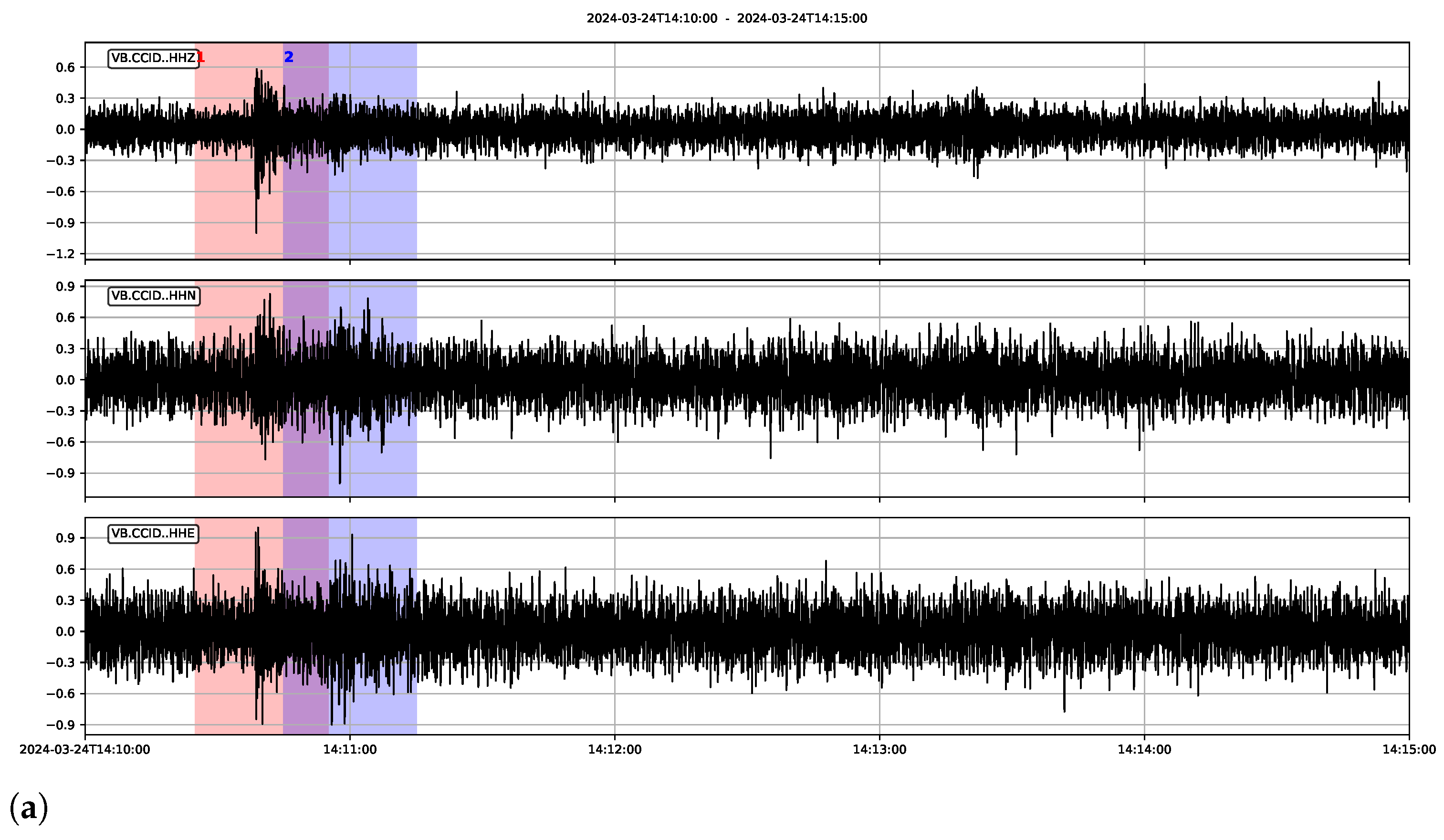
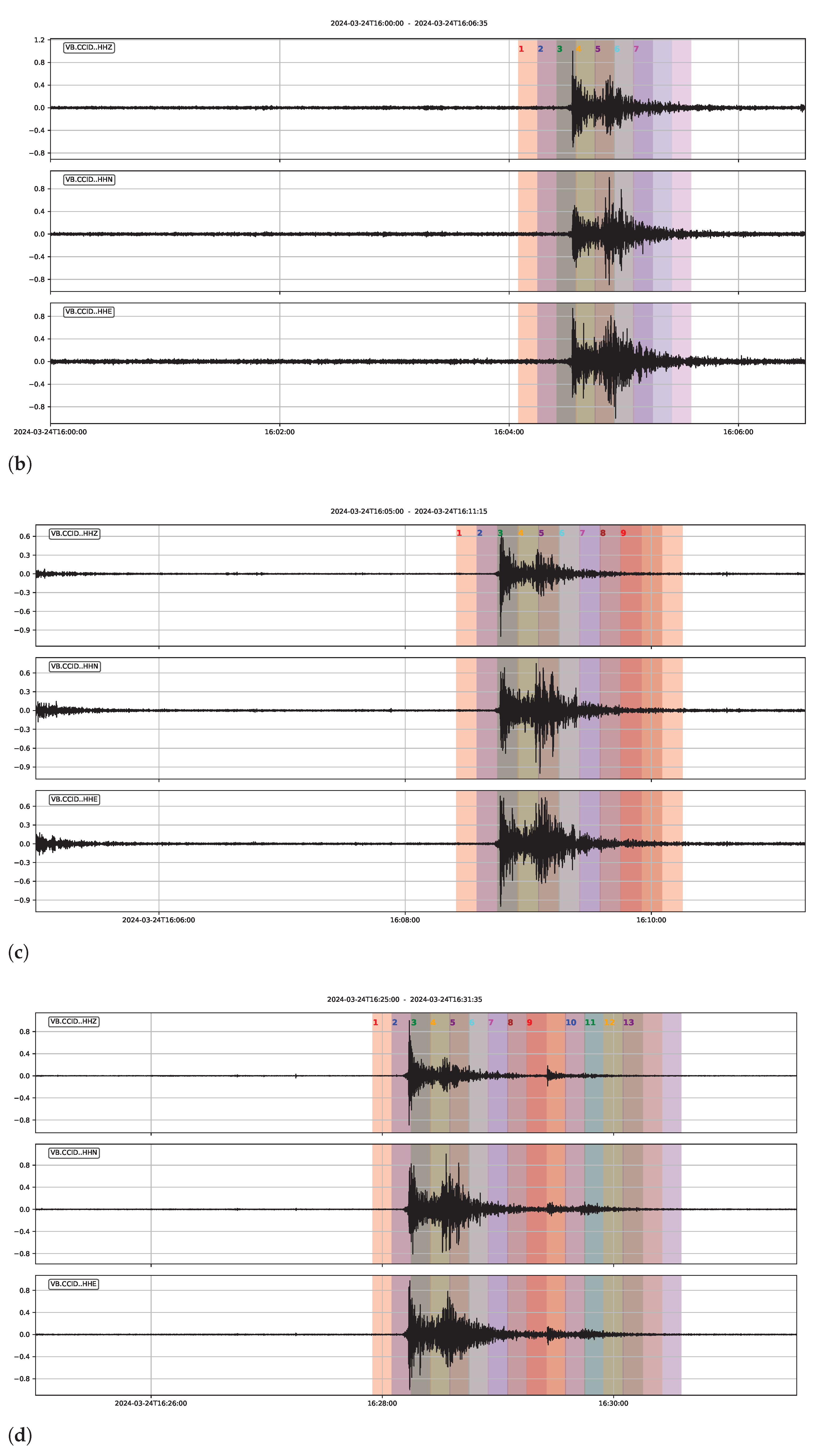
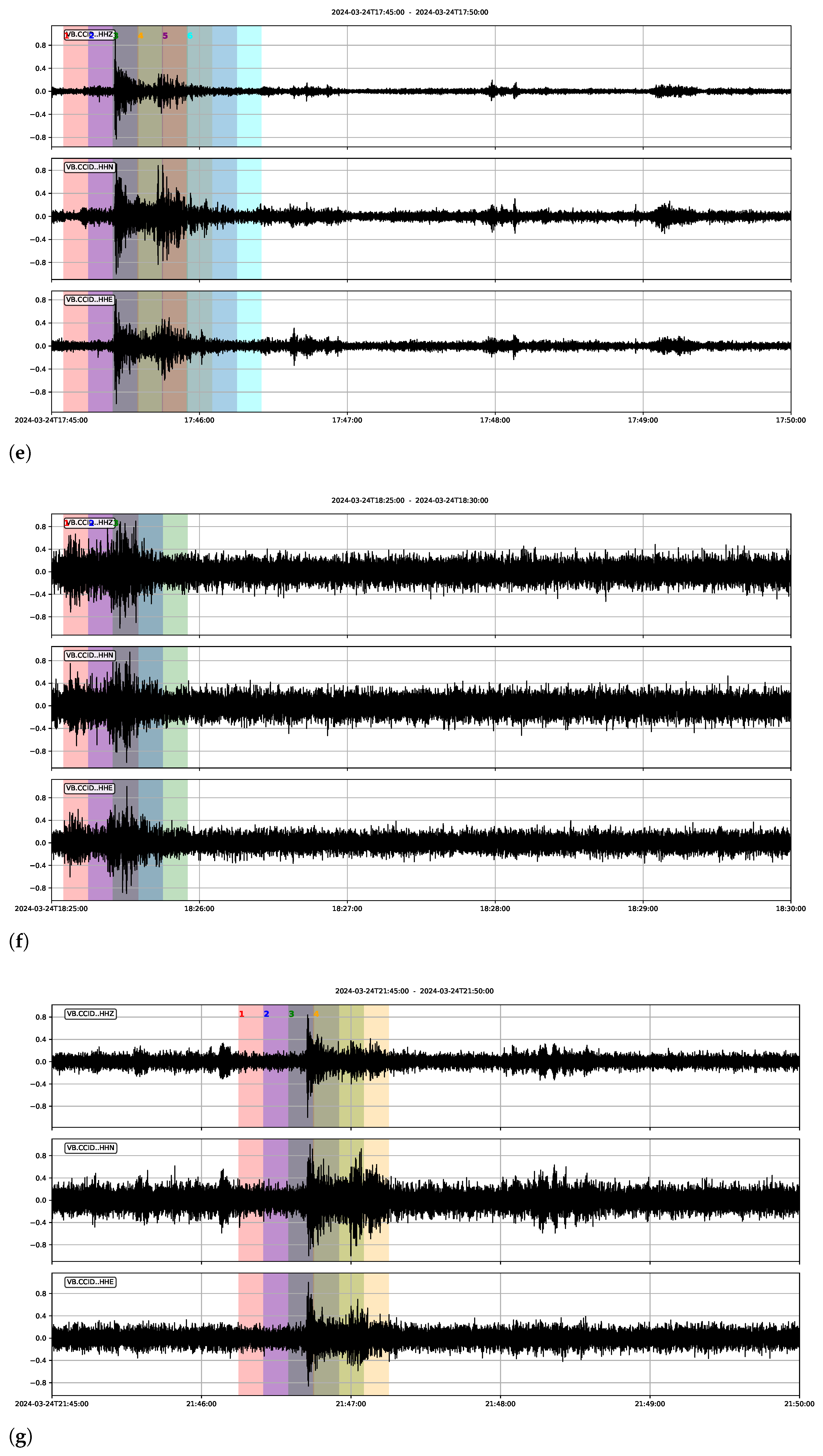
The events that were satisfactorily detected are shown in Figure 15. The traces are shown preprocessed (high-pass filtered at $f_c=2.0$ Hz and scaled to [$-1$, 1]) and represented in 5 min intervals. The 30-s windows in which seismic event content was detected by the algorithm are highlighted in colors and numbered at the top.

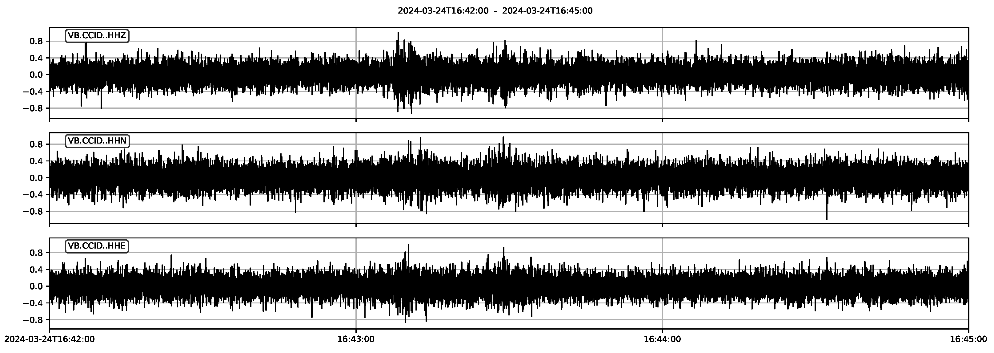
The event vb2024fwyrt from Table 13 was not detected in the CCID recording. Figure 16 shows the traces from the CCID station preprocessed (high-pass filtered at $f_c=2.0$ Hz and scaled to [$-1$, 1]) for the 3 min interval taken around the origin time of this event in which the event is expected to arrive at the station. The event, located between 16:43:00 and 16:44:00, is hardly distinguishable from noise, possibly due to its low magnitude and long distance from the analyzed station.

The two clusters that correspond to the unregistered anthropogenic events picked by the algorithm are shown in Figure 17.

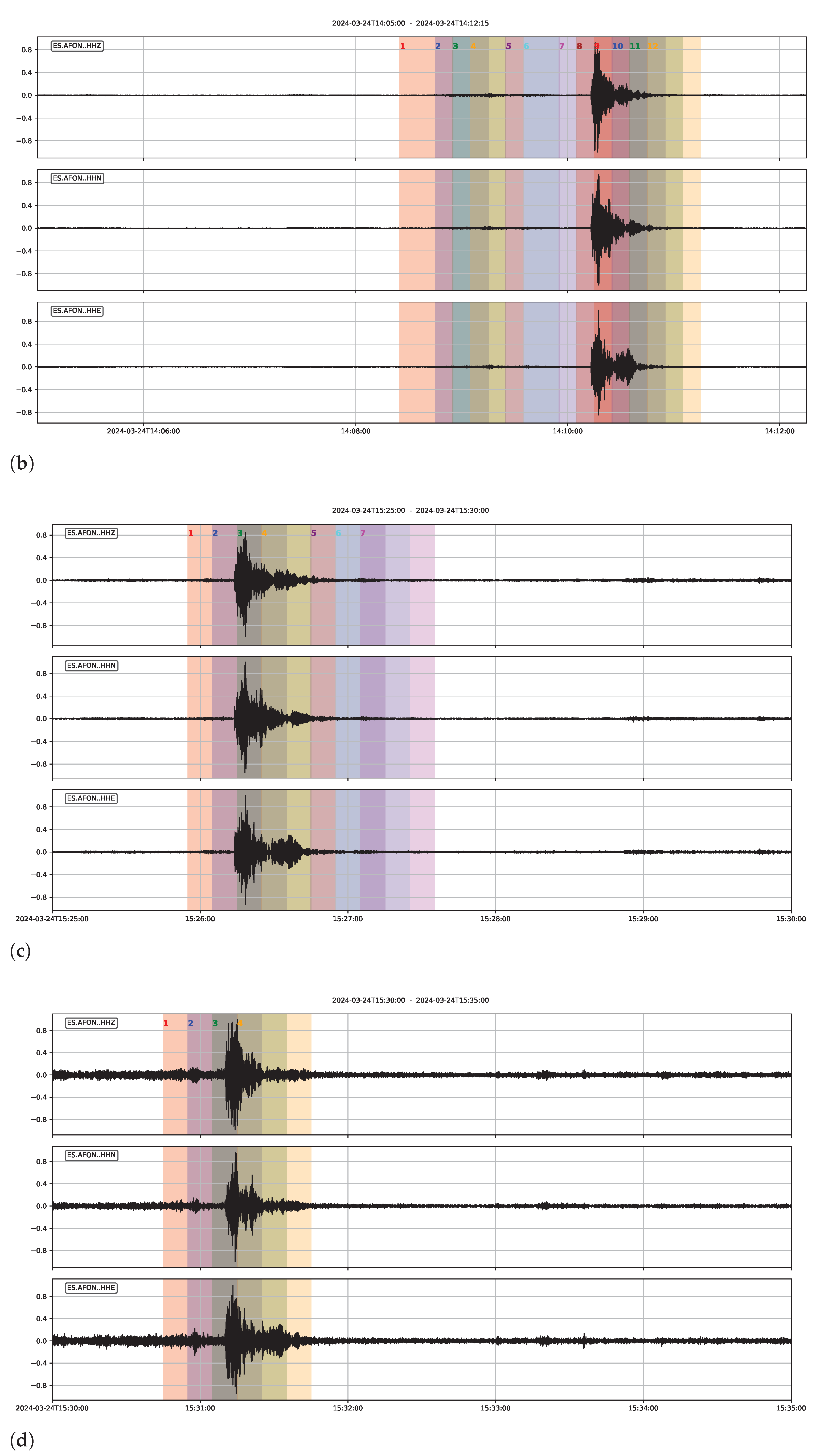
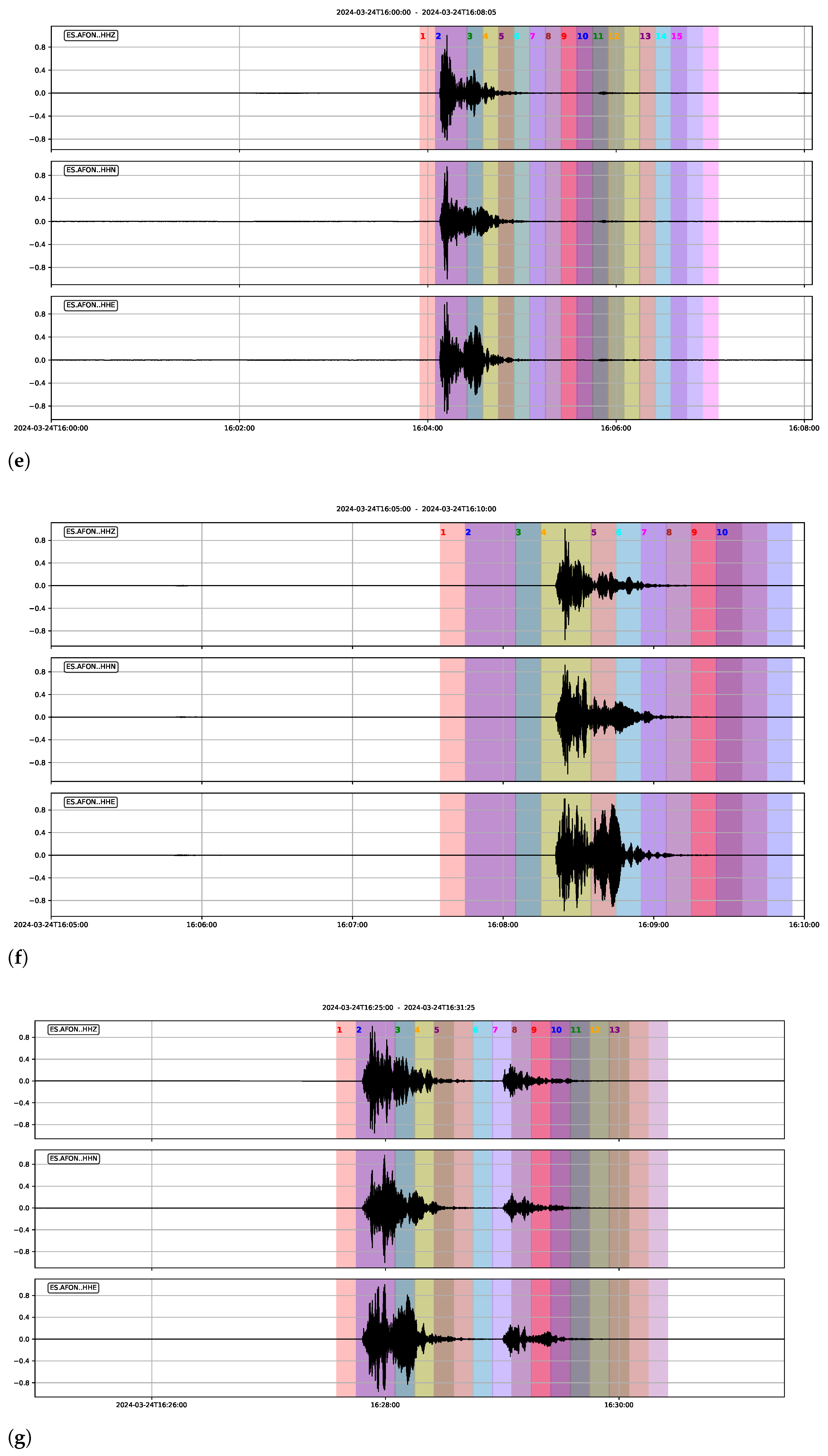
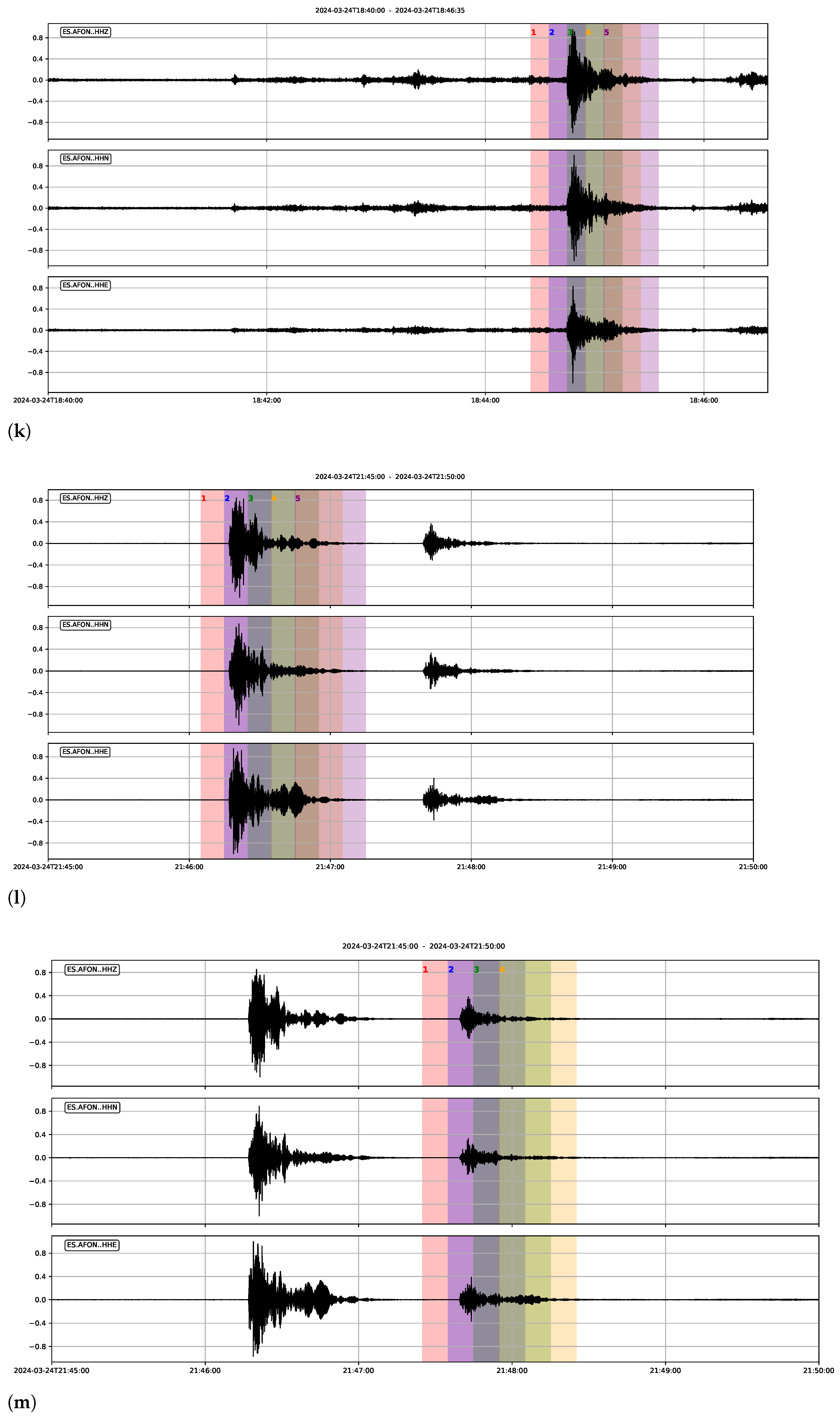
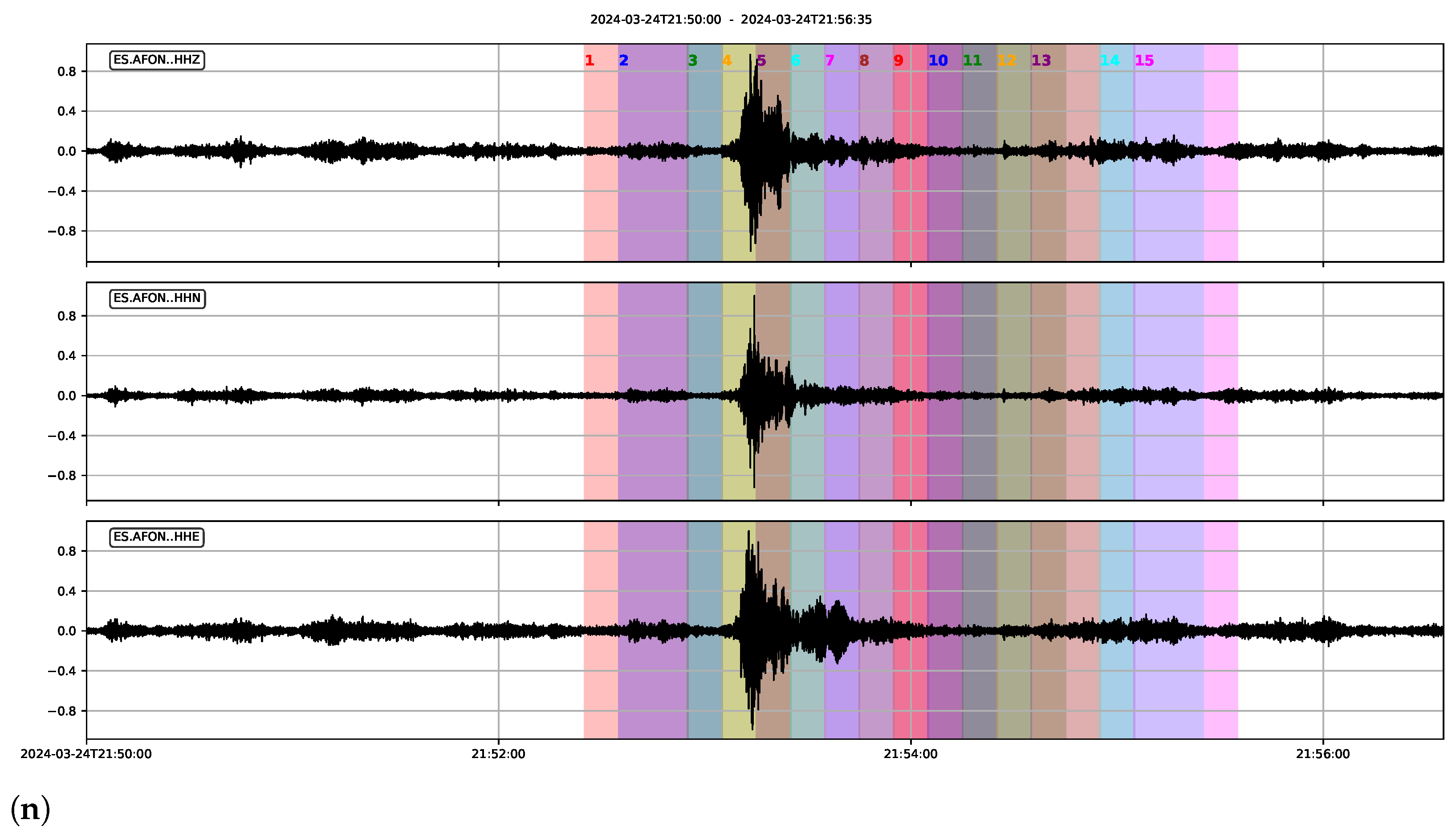
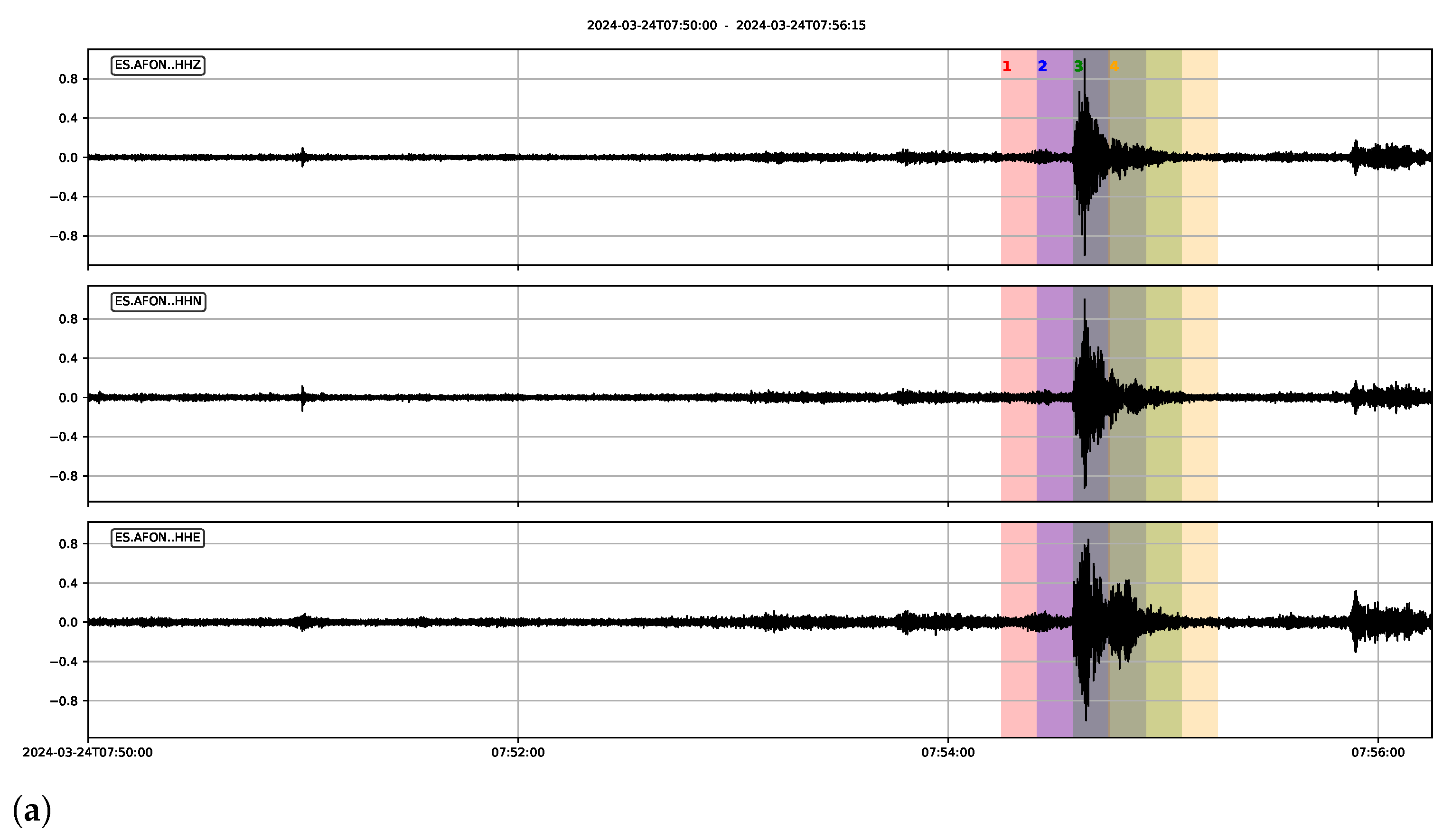
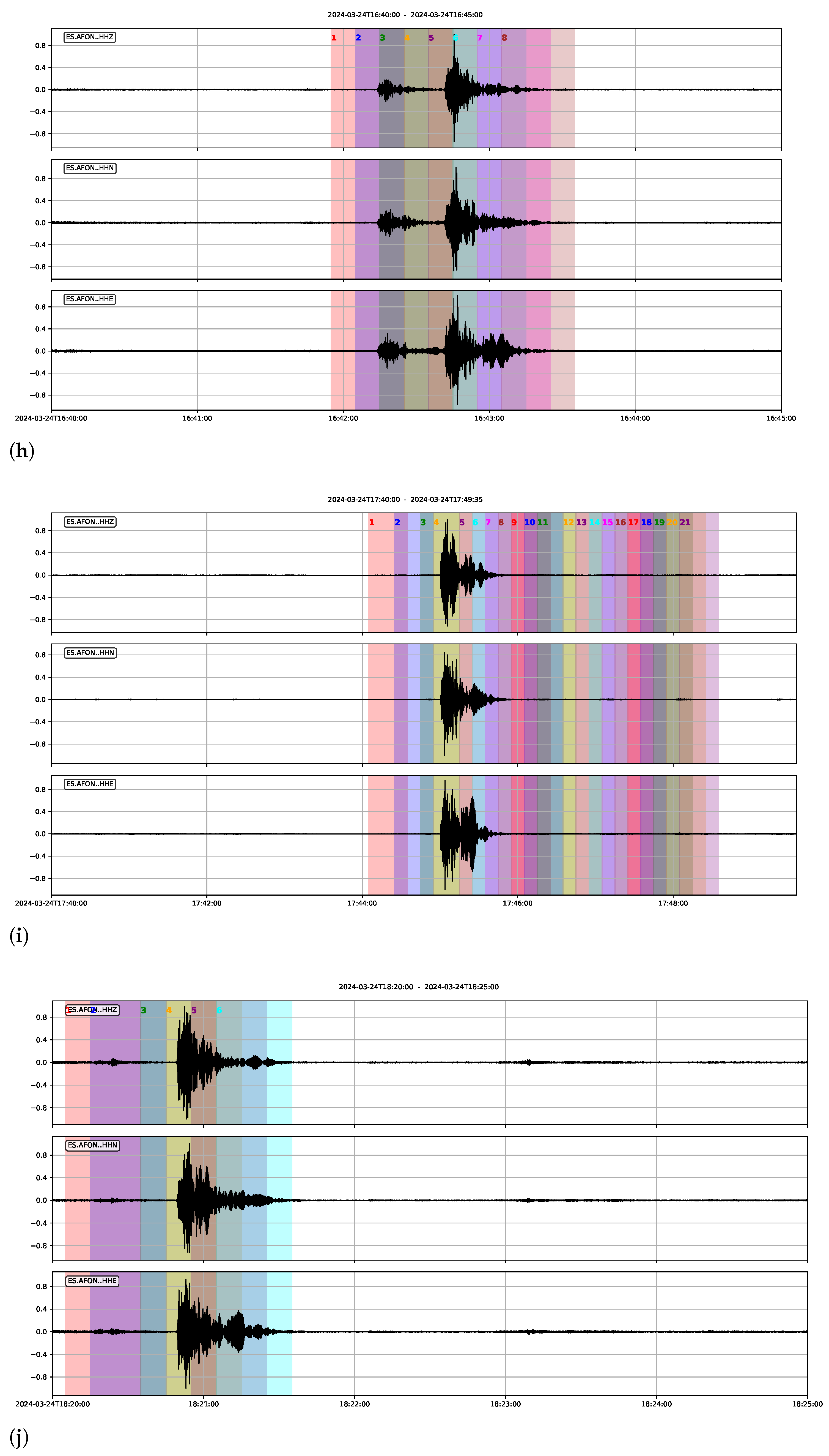
In the continuous recordings from the AFON station, 645 clusters were identified, indicating strong anthropogenic activity on that day. From these, 14 clusters correspond to the earthquake events from Table 13, with all the events picked by AFON successfully identified (2 of the clusters include 2 events). This illustrates the effectiveness of the algorithm in detecting events of interest even in stations operating under strong anthropogenic activity conditions. The clusters with the corresponding detected events are shown in Figure 18.

The remaining 631 clusters contain unregistered anthropogenic events mostly caused by human activity near the location of the AFON station, which demonstrates that the proposed pipeline is highly sensitive to events independently of their nature. As an example, Figure 19 shows one of the clusters that corresponds to an unregistered anthropogenic event picked by the algorithm.

5.5.2. Analysis of the 6 September 2024 Record

The events recorded on 6 September 2024 present a high degree of geographical dispersion. The coordinates of the registered events cover a very wide area. In latitude, they range from the south in Almería/Murcia (${37.80}^{\circ }$) to the north in Castellón/Teruel (${40.49}^{\circ }$). In longitude, they vary from the interior of the Iberian Peninsula (−${1.54}^{\circ }$) to the Mediterranean (+${0.61}^{\circ }$).

Table 14. Details of seismic events recorded on 6 September 2024 and picked by the Lucena del Cid Forest Observatory station.

No.	Event ID	Origin Time	Type	Certainty	Mag.	Picked by
1	vb2024rnjkx	04:21:12	other	suspected	-	CCID
2	vb2024rntkj	09:23:41	quarry blast	known	1.99	CCID
3	vb2024robab	13:14:08	quarry blast	known	-	CCID
4	vb2024rojzt	17:46:31	earthquake	known	2.11	CCID

shows the details of the seismic events registered on 6 September 2024 that were picked by the CCID and AFON stations. They include a suspected unidentified event, 2 confirmed quarry blasts, and a confirmed earthquake. In this case, none of the events were picked by the AFON station.

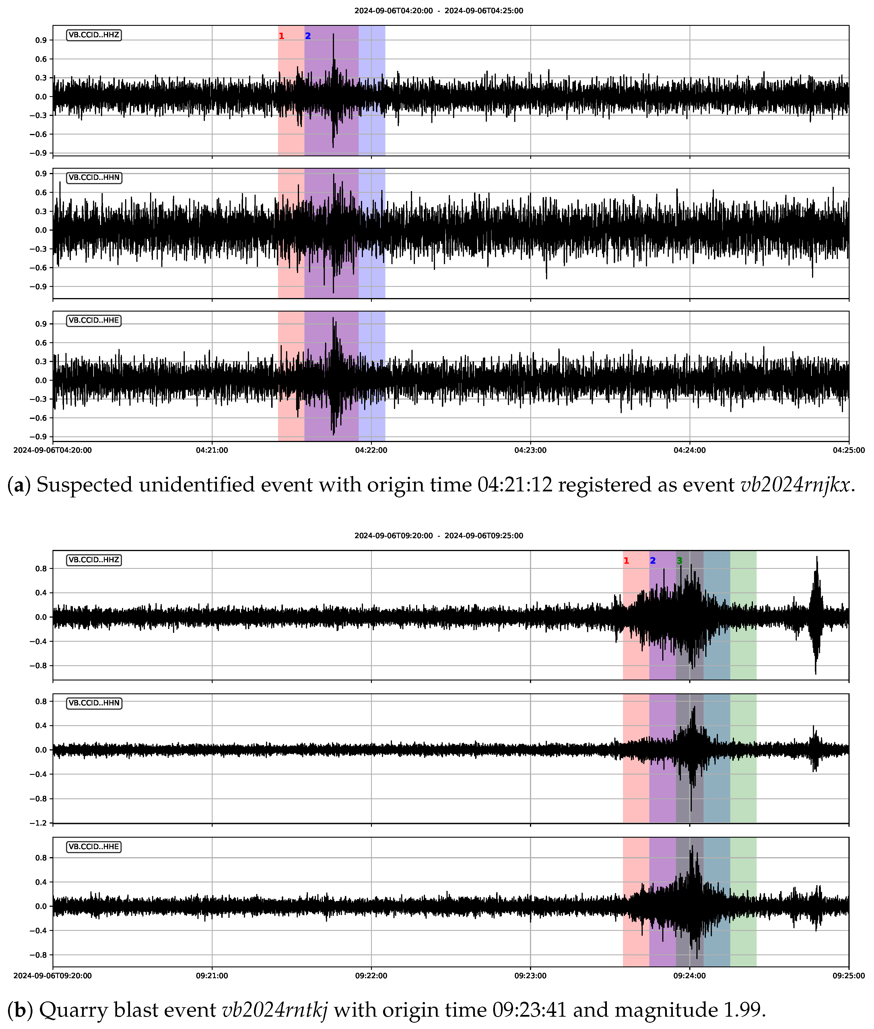
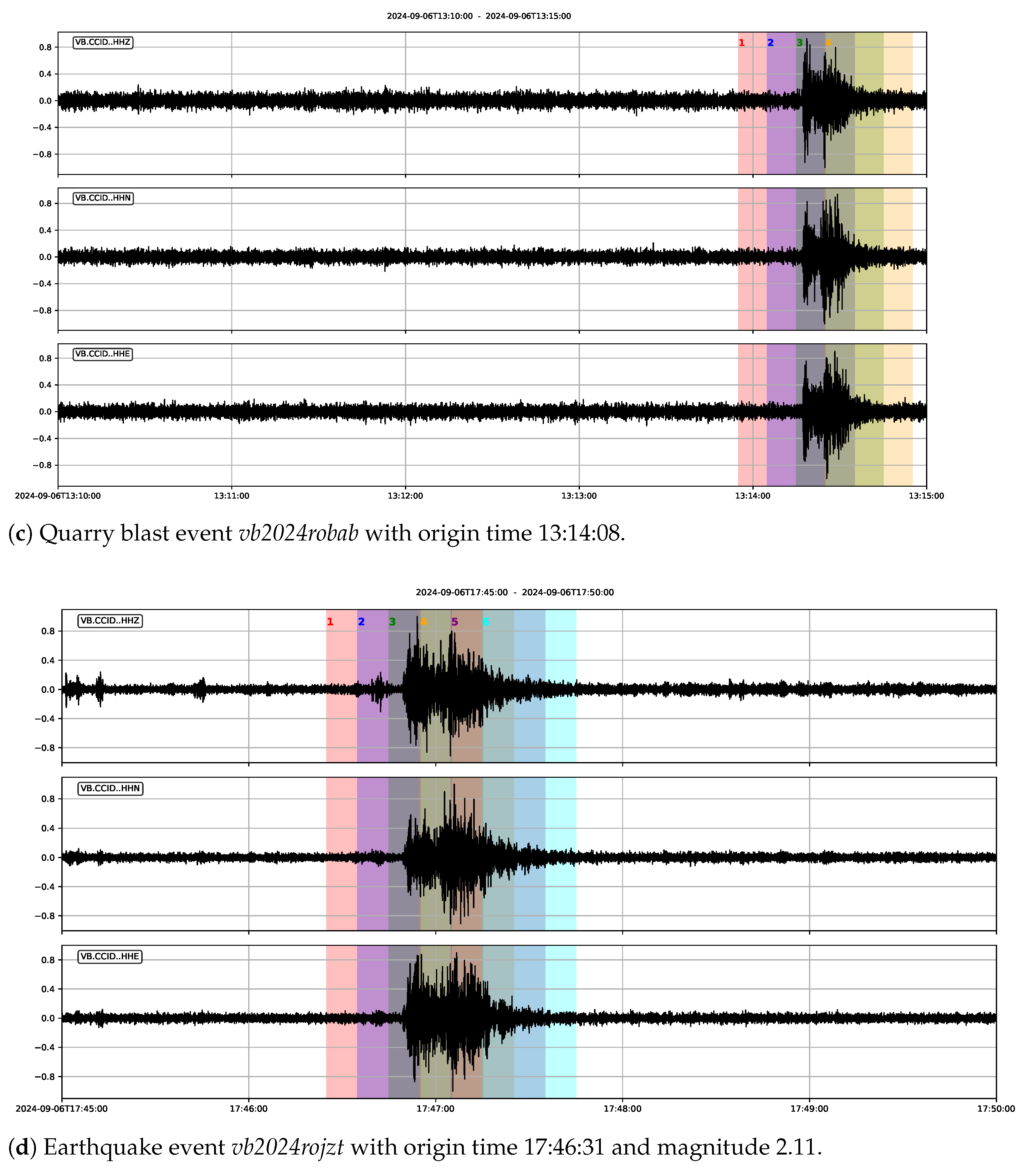
By applying the algorithm to the recordings from this day at the CCID station, like in the previous case, 12 window clusters were identified. From these, 4 clusters correspond to the seismic events from Table 14, with all 4 registered events successfully identified, and 8 are unregistered anthropogenic events. The detection of the registered events is shown in Figure 20.

The 8 clusters that correspond to the unregistered anthropogenic events picked by the algorithm on the recordings from CCID are shown in Figure 21.

In the continuous recordings from the AFON station, 147 clusters were identified, all of them corresponding to unidentified anthropogenic events. This result is consistent with the result obtained in the analysis of the recordings of 24 March 2024, as the AFON station is more susceptible to recording the effects of human activity close by. As an example, Figure 22 shows one of the clusters picked by the algorithm at this station.

These qualitative results confirm the effectiveness of the proposed seismic event detection pipeline and suggest that it can be used not only for earthquake monitoring but also for general seismic monitoring in applications where other types of seismic activity may be of interest.

5.6. Summary and Final Considerations

The main findings from this study are the following:

1.

When trained on known quality signals of $\mathrm{SNR}\ge 6$ dB, the proposed seismic event detection pipeline achieves an accuracy and F1-score of 98.82%, with a precision of 99.05% for the event class, indicating a very low false positive rate on a test data partition of 211 event traces of this quality and 211 noise traces. The accuracy and F1-score degrade to around 93% when event signals of lower $\mathrm{SNR}$ are considered on a bigger test partition of 640 traces (320 event and 320 noise traces) while keeping the event class precision above 99%. This demonstrates that the WST feature representation is highly discriminative for the broadband records from the SISCOVA network.

2.

The proposed method outperforms classical STA/LTA detection methods and the state-of-the-art deep learning models of PhaseNet, EQTransformer, and CRED (in a zero-shot evaluation) even under controlled $\mathrm{SNR}$ conditions. On the matched $\mathrm{SNR}\ge 6$ dB test subset, the classical STA/LTA detector under F1-score optimized thresholding reaches an overall F1-score of 86.73% and event precision of 84.75%. Among the deep learning baselines, EQTransformer under F1-score optimized thresholding is the closest competitor (accuracy and F1 above 92%), yet still exhibits a lower event precision; CRED and PhaseNet achieve overall F1-scores of approximately 83% and 74%, respectively.

3.

Qualitative validation on continuous recordings confirms the operational viability of the proposed pipeline. The pipeline correctly detected the majority of cataloged events during representative continuous full-day recordings from the Lucena del Cid Forest Observatory station. Besides, other anthropogenic events were detected, which are legitimate detection targets given the current scope of the classifier, which treats all seismic sources equally. This outcome supports the practical readiness of the algorithm for the analysis of continuous data streams.

The proposed architecture presents a favorable complexity profile relative to the evaluated deep learning baselines. PhaseNet, EQTransformer, and CRED contain approximately 268K, 376K, and 293K trainable parameters, respectively, whereas the proposed pipeline’s learned component is limited to a single SVM defined by its support vectors and a PCA projection matrix. In contrast, the WST stage requires no learned parameters and is fully determined by its fixed filter bank. Considering all wavelet filter coefficients, the wavelet scattering network used in the proposed method contains fewer than 74K filter coefficients; however, these coefficients do not need to be permanently stored in memory. Since the filter bank can be completely specified by a set of wavelet definitions, the required wavelets can be generated on demand at runtime for each scattering path being evaluated, following an approach similar to that used in [69]. Consequently, the effective memory footprint of the WST stage can be substantially smaller than that suggested by the total number of filter coefficients alone. While formal benchmarking on target embedded hardware has not been conducted in this work and constitutes a key direction of ongoing research, this architectural profile is consistent with deployment on microcontroller-class platforms and motivates future hardware validation work.

6. Conclusions

The results obtained from the Valencian Community Seismic Network (SISCOVA) data demonstrate that wavelet scattering-based feature extraction combined with classical machine learning can achieve high seismic event detection performance while maintaining a very low false positive rate. The proposed approach consistently outperformed both the STA/LTA baseline and the evaluated zero-shot deep learning models, while also demonstrating practical applicability to continuous seismic recordings.

Future work will focus on three directions: (i) fine-grained discrimination between natural earthquakes and anthropogenic seismic sources such as quarry blasts, which the current pipeline intentionally treats as a single event class; (ii) extension of the pipeline to incorporate phase picking and source parameter estimation; and (iii) deployment of the detection algorithm on embedded hardware platforms for real-time, on-site inference within the SISCOVA network.