Enhancing the Explainability of the MRI-Based Brain Tumour Detection with Image Preprocessing

Abstract

Accurate and interpretable brain tumour detection from magnetic resonance imaging (MRI) is important for the reliable use of computer-assisted diagnostic systems. This study examines whether image preprocessing can improve the localisation quality of explanations generated by convolutional neural network (CNN) classifiers while preserving high classification performance. Two pre-trained CNN architectures, ResNet50 and DenseNet121, were fine-tuned using the BRISC 2025 dataset, which contains 6000 annotated contrast-enhanced T1-weighted MRI images: 5000 training images and 1000 test images. The dataset includes four classes: glioma, meningioma, pituitary tumour, and healthy brain images. The original classification layers were replaced with custom fully connected heads designed for four-class classification. Model explanations were generated using Grad-CAM, Integrated Gradients, and LIME. Their localisation quality was evaluated against the available tumour segmentation masks using Intersection over Union (IoU), the Dice coefficient, and the Pointing Game metric. Tests show that both models (99.1% for ResNet50 and 99.2% for DenseNet121) perform well in terms of validation accuracy, but the explanation maps often operate in regions outside the clinically relevant area. To combat this issue, an image preprocessing pipeline utilising Otsu threshold masking, hole filling, and brightness–contrast jittering was implemented to filter noise from the background and isolate the focus area—brain region. After preprocessing, the validation accuracy of the DenseNet121 model was 99.6%, and the average Grad-CAM explainability metrics improved from 21.49% to 23.08% IoU, from 30.21% to 32.49% Dice coefficient, and from 48.33% to 51.67% Pointing Game score. The results indicate that conventional image preprocessing can moderately improve the spatial agreement between explanation maps and annotated tumour regions without reducing classification accuracy.

1. Introduction

Brain tumours are among the most serious neurological diseases and may be life-threatening, often leading to severe impairments of cognitive, sensory, and motor functions. Early and accurate diagnosis is essential for selecting appropriate treatment strategies and improving patient management. Magnetic resonance imaging (MRI) is one of the primary imaging modalities for brain tumour diagnosis because it provides excellent soft-tissue contrast and high spatial resolution without exposing patients to ionising radiation [1,2].

In recent years, artificial intelligence (AI), particularly deep learning (DL), has become an important tool in medical image analysis. Convolutional neural networks (CNNs) have achieved remarkable performance in MRI-based tumour classification, segmentation, and localisation tasks [3,4,5,6]. Transfer learning approaches based on pre-trained architectures such as ResNet and DenseNet have shown excellent performance in brain tumour classification by exploiting hierarchical image features learned from large-scale image datasets [7,8,9].

Despite these advances, the reliability and transparency of CNN-based medical decision systems remain important challenges. Most deep learning models operate as “black boxes”, providing highly accurate predictions without indicating which image regions contributed to the final decision [10]. This lack of interpretability limits the clinical acceptance of artificial intelligence-assisted diagnostic systems, particularly when activation maps extend beyond anatomically relevant tumour regions [11].

To improve model interpretability, explainable artificial intelligence (XAI) techniques have been increasingly adopted in medical imaging. Post hoc methods such as Gradient-weighted Class Activation Mapping (Grad-CAM), Integrated Gradients, and Local Interpretable Model-agnostic Explanations (LIME) are widely used to visualise the image regions influencing CNN predictions [12,13]. These methods provide qualitative information about whether the model focuses on tumour tissue or on irrelevant background structures and imaging artefacts.

Although numerous studies have reported excellent classification performance for brain tumour detection, quantitative evaluation of explainability and localisation reliability remains relatively limited. In addition, while image preprocessing has been widely used to improve classification performance, its influence on explainability has received considerably less attention. Background artefacts, intensity variations, and non-brain regions may unintentionally affect CNN activations and reduce the reliability of the generated explanation maps.

In this context, the present study investigates whether image preprocessing can improve the localisation reliability of explainability methods while preserving the high classification performance of CNN-based brain tumour classifiers. Two widely used transfer learning architectures, ResNet50 and DenseNet121, were fine-tuned using the BRISC 2025 MRI dataset, which contains glioma, meningioma, pituitary tumour, and healthy brain images.

Model explainability was analysed using Grad-CAM, Integrated Gradients, and LIME, whereas localisation quality was quantitatively evaluated using IoU, Dice coefficient, and Pointing Game metrics computed from the available tumour segmentation masks. To eliminate irrelevant background regions and lessen the impact of image artefacts, a preprocessing pipeline including Otsu threshold masking, binary hole filling, and brightness–contrast jittering was applied.

The study investigates how conventional MRI preprocessing influences the localisation behaviour of widely used explainability methods and examines the relationship between classification performance and explainability reliability.

Although image preprocessing and explainability methods have been extensively investigated independently, their combined influence on the localisation reliability of CNN explanations has received considerably less attention. Unlike previous studies that primarily report classification performance or qualitative explainability results, the present work quantitatively evaluates how conventional MRI preprocessing affects the spatial consistency of Grad-CAM, Integrated Gradients, and LIME using expert-annotated tumour segmentation masks and multiple localisation metrics.

The main contributions of this work are as follows:

• Fine-tuning and evaluation of ResNet50 and DenseNet121 for four-class MRI brain tumour classification using the BRISC 2025 dataset.
• Quantitative evaluation of explainability localisation using Grad-CAM, Integrated Gradients, LIME, Intersection over Union (IoU), Dice coefficient, and Pointing Game metrics.
• Investigation of the influence of conventional MRI preprocessing on the localisation reliability of CNN explanation maps.
• Comparative analysis of explainability performance across different brain tumour classes.

The remainder of this paper is organised as follows. Section 2 reviews related work in brain tumour classification and explainable AI for medical imaging. Section 3 describes the materials and methods, including the dataset, preprocessing pipeline, CNN architectures, and evaluation methodology. Section 4 presents the experimental and explainability results. Section 5 discusses the limitations of the study, while Section 6 concludes the paper and outlines future research directions.

2. Related Work

2.1. Deep Learning Approaches for Brain Tumour Classification

Deep learning has become one of the leading approaches for MRI-based brain tumour analysis because of its ability to automatically learn complex image representations and improve diagnostic performance. Convolutional neural networks (CNNs) are widely used for tumour classification, segmentation, and localisation tasks in medical imaging [2,3,4,5,6].

Transfer learning based on pre-trained CNN architectures has shown excellent performance in brain tumour classification. Architectures such as ResNet, DenseNet, VGG, EfficientNet, and MobileNet have been successfully adapted to MRI datasets for the classification of glioma, meningioma, pituitary tumours, and healthy brain images [7,8,9,10,11,12,13,14]. In addition to conventional transfer learning, ensemble and hybrid approaches combining CNNs with optimisation algorithms or traditional machine learning classifiers have also been investigated to improve feature extraction and classification robustness [15,16,17,18].

Despite the high classification performance reported in the literature, considerably less attention has been devoted to the interpretability of CNN models and the reliability of their localisation behaviour. Direct comparison between published studies is often difficult because different datasets, evaluation protocols, preprocessing strategies, and class distributions are used. Many studies are also limited by relatively small datasets, the absence of external validation, or the potential risk of model overfitting. Furthermore, several publications rely on publicly available datasets without providing sufficient information about the data sources or patient distribution, making direct comparison between studies even more difficult.

2.2. Segmentation and Localisation Methods

Segmentation is fundamental to medical image analysis, as it supports the identification and delineation of pathological regions, facilitating disease localisation and clinical interpretation. Segmentation-based approaches in brain tumour analysis have been mainly applied to detect tumour borders and distinguish pathological tissue from healthy brain structures [19].

Traditional image segmentation techniques include thresholding, clustering, and region-growing methods. More recently, deep learning approaches based on Fully Convolutional Networks (FCNs), U-Net architectures, and Mask R-CNN have become the dominant solutions for medical image segmentation [20]. Accurate segmentation masks are particularly valuable for assessing localisation quality and determining whether CNN-based classification models focus on clinically relevant tumour regions.

However, in many MRI classification studies, segmentation masks are used solely for dataset annotation and are not used to quantitatively assess whether explainability maps correspond to the annotated tumour regions. As a result, the reliability of localisation remains insufficiently assessed, limiting the interpretability and clinical trustworthiness of black-box classification models.

2.3. Explainable AI in Medical Imaging

The growing use of deep learning in healthcare has increased the need for models whose decisions can be understood and interpreted. Explainable artificial intelligence (XAI) addresses this problem by providing methods that help explain how complex models reach their predictions, making their use more reliable in clinical practice [21].

XAI methods are generally divided into global and local approaches, as well as model-specific and model-agnostic methods. In medical imaging, local post hoc methods are used more often because they highlight the image regions that influence the prediction for an individual case [22].

Gradient-weighted Class Activation Mapping (Grad-CAM) is one of the most commonly used explainability methods for CNN-based medical image analysis. It generates heatmaps showing which image regions contribute most to the final classification [23]. Another widely used method is Local Interpretable Model-agnostic Explanations (LIME), which explains the behaviour of black-box models by fitting simple interpretable models around individual predictions [24].

Most studies using Grad-CAM or LIME evaluate the generated heatmaps visually. Fewer studies perform a quantitative evaluation using localisation metrics such as Intersection over Union (IoU), the Dice coefficient, and the Pointing Game. Recent review papers have emphasised the need to combine quantitative evaluation with clinical validation to better assess the reliability of explainable AI methods in medical imaging [25,26,27,28,29]. However, the influence of image preprocessing on the localisation quality of explanation maps in MRI-based brain tumour classification has rarely been investigated.

2.4. Research Gap and Motivation

Many deep learning methods have reported excellent results for MRI-based brain tumour classification. However, fewer studies have examined whether the explanation maps generated by these models accurately correspond to the tumour regions identified by experts. Most existing work still relies mainly on visual inspection instead of quantitative localisation analysis.

Image preprocessing is widely used to improve classification performance, but its influence on explainability has received much less attention. Background artefacts, intensity variations, and non-brain regions may affect CNN activations and reduce the reliability of the generated explanation maps.

Another limitation is that explainability is rarely evaluated using localisation metrics such as Intersection over Union (IoU), the Dice coefficient, and the Pointing Game. As a result, high classification accuracy does not necessarily mean that the model is focusing on the tumour itself.

This study investigates whether conventional MRI preprocessing can improve the localisation reliability of CNN explanation maps while preserving high classification performance. Rather than introducing a new preprocessing algorithm, we evaluate how standard preprocessing steps influence explainability localisation by combining transfer learning, three widely used XAI methods, and quantitative localisation metrics. The goal is to better understand the relationship between classification accuracy and the localisation reliability of explanation maps.

3. Materials and Methods

3.1. BRISC Dataset

The experiments were carried out using the Brain Research Innovation with Segmentation and Classification (BRISC 2025) dataset [1]. The dataset contains 6000 contrast-enhanced T1-weighted MRI brain images acquired in axial, sagittal, and coronal planes, including 5000 training images and 1000 test images. Four classes are included in the dataset: glioma, meningioma, pituitary tumour, and healthy brain images (no-tumour class). In addition to the class labels, BRISC 2025 provides expert-annotated tumour segmentation masks, which were used to evaluate the localisation quality of the generated explanation maps. The class distribution of the training and test subsets is presented in

Table 1. Class distribution of the BRISC 2025 dataset.

Class	Training Subset		Test Subset
	Count	%	Count	%
Glioma	1147	22.94%	254	25.4%
Meningioma	1329	26.58%	306	30.6%
Pituitary tumour	1457	29.14%	300	30%
No tumour	1067	21.34%	140	14%

. The available tumour segmentation masks make it possible to compare the generated explanation maps directly with the annotated tumour regions using quantitative localisation metrics.

All MRI images were zero-padded to a fixed resolution of 512 × 512 pixels in order to maintain consistent input dimensions, and then additional preprocessing was used to remove background noise. Since the employed CNN architectures were pre-trained on ImageNet, the images were subsequently converted to the RGB colour space. Finally, ImageNet normalisation statistics were applied to ensure compatibility with the pre-trained backbone weights.

The dataset does not provide a validation subset; thus, for the main evaluation, the test set was used as the validation set. Later, to evaluate the robustness of the derived models, a 5-fold stratified cross-validation was used, with each fold having 1000 images as a validation set, where the test set was not used. The test set is used for the final model evaluation. All preprocessing and normalisation procedures were applied after dataset splitting in order to minimise potential data leakage between subsets. The training subsets were further augmented to increase the robustness of the models. The segmentation masks were not used during model training and served exclusively for explainability evaluation using localisation-based metrics.

The BRISC dataset is publicly available through the Kaggle platform [1]. The present study used only anonymised publicly available MRI data and therefore did not require additional ethical approval.

3.2. Data Preprocessing

A preprocessing pipeline was introduced to reduce the influence of background regions and image artefacts on the explainability behaviour of the CNN models. Preliminary Grad-CAM visualisations showed that the models frequently produced activations outside the brain region, particularly near the image borders and background. To reduce these unwanted activations, several preprocessing steps were applied before model training.

First, Otsu thresholding was used to separate the brain from the background. Otsu’s method automatically determines a threshold by minimising the intra-class variance between foreground and background pixel intensities [30]. In contrast-enhanced T1-weighted MRI images, the intensity difference between the brain and the surrounding background is usually sufficient for reliable foreground extraction. The purpose of this step is simply to remove the background before CNN training rather than to perform anatomical tissue segmentation. More complex methods, such as Multi-Otsu or adaptive thresholding, were not investigated because separating different tissue types was outside the scope of this work.

After thresholding, small holes occasionally remained inside the extracted brain region. These were removed using the binary_fill_holes function from the SciPy library [31]. The algorithm identifies background pixels connected to the image border and fills only the enclosed regions inside the binary mask. As a result, a continuous foreground mask is obtained while preserving the outer boundary of the brain.

During training, moderate brightness and contrast jittering (±5%) was applied to improve robustness to small variations in MRI acquisition conditions. More aggressive augmentation techniques were intentionally avoided because they may alter tumour morphology and influence the localisation behaviour of the explainability methods. The selected augmentation strategy, therefore, improves robustness while preserving the anatomical appearance of the MRI images.

After preprocessing, all images were normalised using the standard ImageNet normalisation statistics before being used for training and evaluation. All preprocessing and normalisation steps were performed after dataset partitioning to avoid data leakage between the training and validation subsets.

The preprocessing methods used in this study are standard image processing techniques. The novelty of the proposed framework lies in the quantitative evaluation of how these preprocessing steps influence explainability, localisation and localisation reliability in CNN-based brain tumour classification. The complete preprocessing workflow is illustrated in Figure 1.

3.3. CNN Architectures

Two convolutional neural network architectures, ResNet50 [7] and DenseNet121 [8], pre-trained on the ImageNet dataset, were employed for MRI brain tumour classification. Transfer learning was used to adapt feature representations learned from large-scale natural image datasets to the medical imaging domain.

The backbone networks were used without structural modifications. Since the PyTorch implementation applies global average pooling before the final fully connected layers, the models can process 512 × 512 pixel images directly. This avoids reducing the image resolution before classification, but requires more GPU memory and longer training time.

The original classification layers were replaced with a fully connected classification head designed for the four-class classification problem (glioma, meningioma, pituitary tumour, and healthy brain). The classification head consisted of three fully connected layers with 256, 64, and 4 neurons, respectively. Batch normalisation was applied after each hidden layer, while the final layer used a Softmax activation function to produce class probabilities.

The same classification head was used for both CNN architectures to ensure a fair comparison. During training, the backbone layers were fine-tuned using a lower learning rate, whereas the newly added classification layers were trained with a higher learning rate. Model optimisation was performed using the Adam optimiser and categorical cross-entropy loss. The complete transfer learning framework is shown in Figure 2.

3.4. Training Procedure

The CNN models were trained on the BRISC 2025 dataset using transfer learning. Training was carried out for 25 epochs with a batch size of 32. In our experiments, the validation loss stabilised within this training period, and the last epochs did not lead to a noticeable improvement.

The Adam optimiser was used during training. The newly added classification head was trained with a learning rate of 1 × 10⁻³, whereas the pre-trained backbone was fine-tuned using a lower learning rate of 1 × 10⁻⁴.

Categorical cross-entropy was used as the loss function for the four-class classification task. The model with the highest validation accuracy was selected for the subsequent explainability analysis.

The experiments were implemented in Python 3.8 using PyTorch 2.4.1 + cu121. Training and explainability analysis were performed on a workstation equipped with an NVIDIA RTX 4090 GPU (24 GB) running under Windows Subsystem for Linux (WSL) with CUDA 12.6.1 and cuDNN 9.7.0.

3.5. Explainability Methods

Three post hoc explainability methods were used in this study: Gradient-weighted Class Activation Mapping (Grad-CAM) [32], Local Interpretable Model-agnostic Explanations (LIME) [33], and Integrated Gradients [34].

Grad-CAM is a model-specific method developed for convolutional neural networks. It generates heatmaps by computing the gradients of the target class with respect to the feature maps of the last convolutional layer. These heatmaps indicate the image regions that contribute most to the final prediction.

LIME is a model-agnostic explainability method. It explains the prediction of a black-box model by perturbing different image regions and analysing how these perturbations affect the predicted class. The contribution of each region is then estimated using an interpretable surrogate model [33].

Integrated Gradients estimates the contribution of each input pixel by integrating the gradients between a baseline image and the original input image. The resulting attribution map highlights both positive and negative pixel contributions to the final prediction [34].

The explanation maps were generated using the validation subset of the BRISC dataset. Grad-CAM, Integrated Gradients, and LIME were implemented using the following Python libraries:

• Grad-CAM: TorchCAM [35];
• Integrated Gradients: Captum [36];
• LIME: LIME [33].

Before quantitative evaluation, all explanation maps were normalised to the range [0, 1] using min–max normalisation and converted into binary localisation masks using a fixed threshold of 0.5. The same threshold was applied to all explainability methods and CNN architectures.

Localisation metrics were calculated only for tumour-containing images because no reference tumour mask was available for the no-tumour class. The binary localisation masks were then compared with the corresponding tumour segmentation masks using Intersection over Union (IoU), the Dice coefficient, and the Pointing Game.

The explainability analysis was performed to determine whether the CNN models focused on the annotated tumour regions or on unrelated image structures during classification.

3.6. Evaluation Metrics

Two metrics were used to evaluate the classification performance of the CNN models: validation accuracy and the F1-score. Validation accuracy shows how many MRI images were classified correctly, while the F1-score combines precision and recall into a single measure. Both metrics were calculated using the validation subset.

In addition to the classification results, explainability was evaluated using three localisation metrics: Intersection over Union (IoU), the Dice coefficient, and the Pointing Game. These metrics were calculated by comparing the generated explanation maps with the corresponding tumour segmentation masks provided in the BRISC dataset.

Intersection over Union (IoU) measures the overlap between the explanation map AAA and the corresponding tumour segmentation mask BBB, and is defined as

$$IoU={\displaystyle \frac{\left|A\cap B\right|}{\left|A\cup B\right|}}$$

(1)

The Dice coefficient measures the similarity between the explainability activation region and the annotated tumour region:

$$Dice={\displaystyle \frac{2\left|A\cap B\right|}{\left|A\right|+\left|B\right|}}$$

(2)

The Pointing Game evaluates whether the pixel with the highest activation falls inside the annotated tumour region.

Higher IoU, Dice coefficient, and Pointing Game values indicate better agreement between the explanation maps and the annotated tumour regions. All reported localisation metrics correspond to the average values calculated over the validation subset.

4. Results

4.1. Classification Results

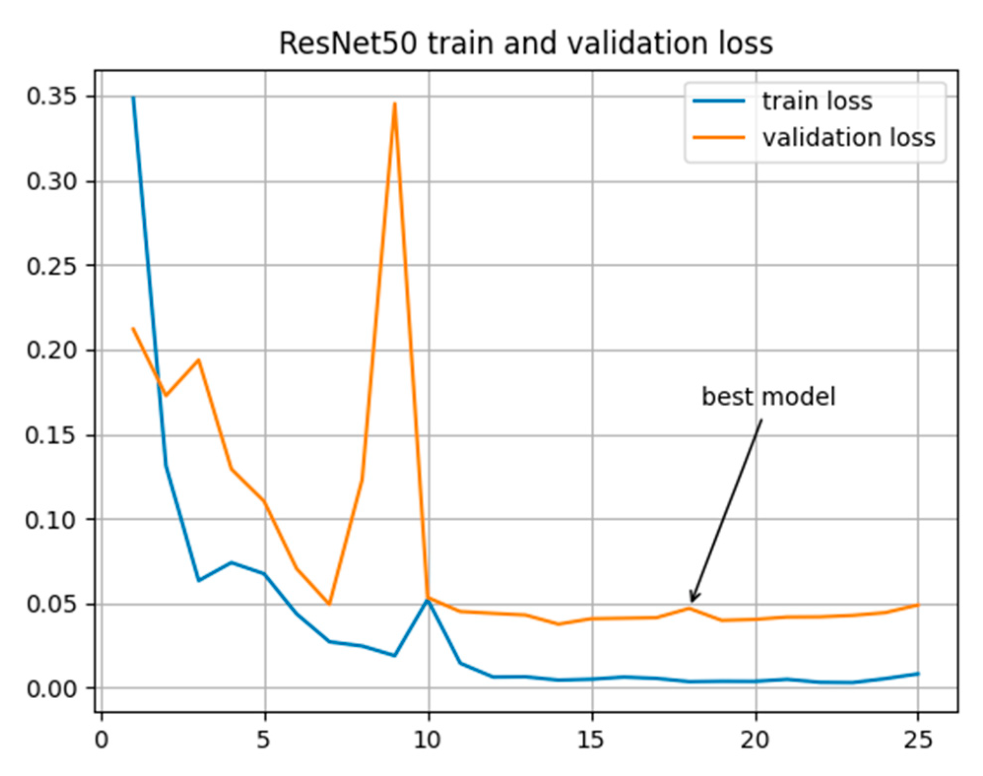
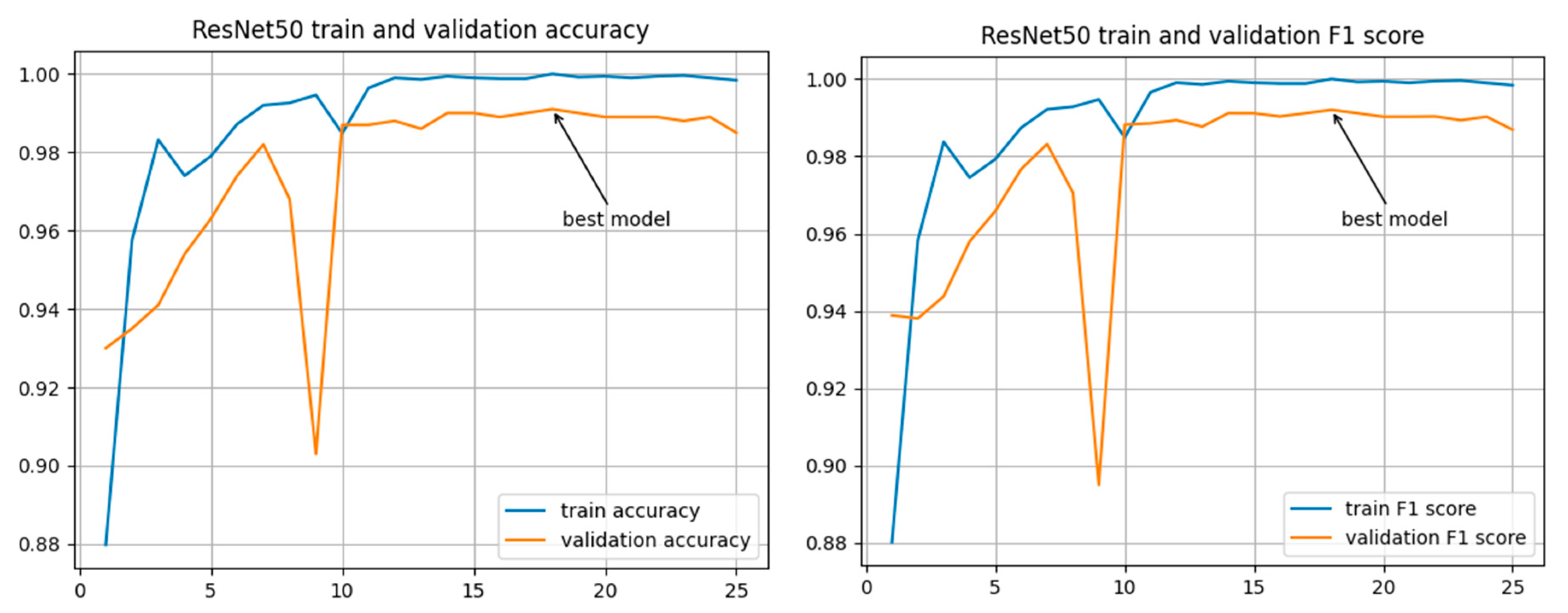
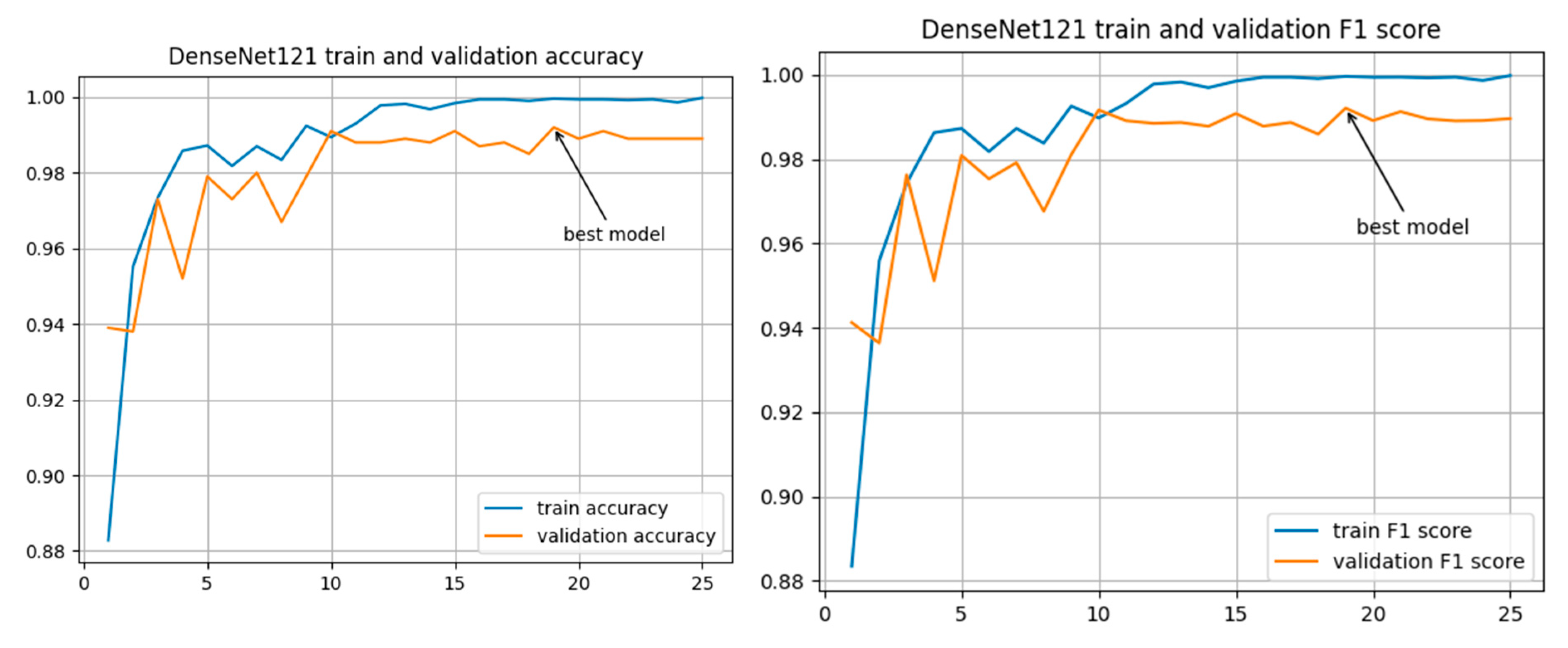
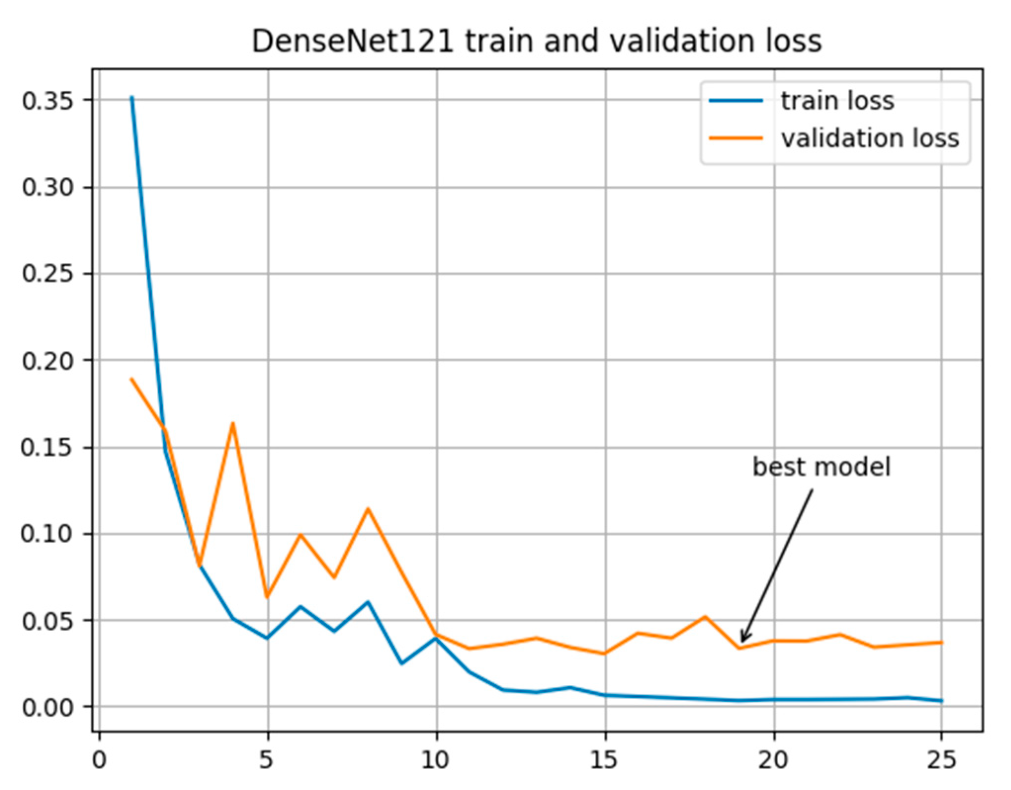
The classification performance of the fine-tuned ResNet50 and DenseNet121 models was evaluated using the BRISC validation subset. Figure 3 show the training and validation loss curves, while Figure 4 present the corresponding validation accuracy and F1-score curves. Figure 5 shows the training and validation loss curves for the DenseNet121 model. Figure 6 presents the corresponding validation accuracy and F1-score curves.

ResNet50 achieved a validation accuracy of 99.1% after 18 training epochs, whereas DenseNet121 achieved 99.2% after 19 epochs. The F1-score followed the same trend as the validation accuracy for both models throughout training.

The high classification performance of both CNN architectures allowed them to be used for the explainability experiments described in the following sections.

Both CNN architectures achieved high classification accuracy on the BRISC dataset. ResNet50 achieved a maximum validation accuracy of 99.1%, whereas DenseNet121 achieved 99.2%. As both models performed similarly, they were used in the subsequent explainability experiments.

4.2. Cross-Validation Analysis

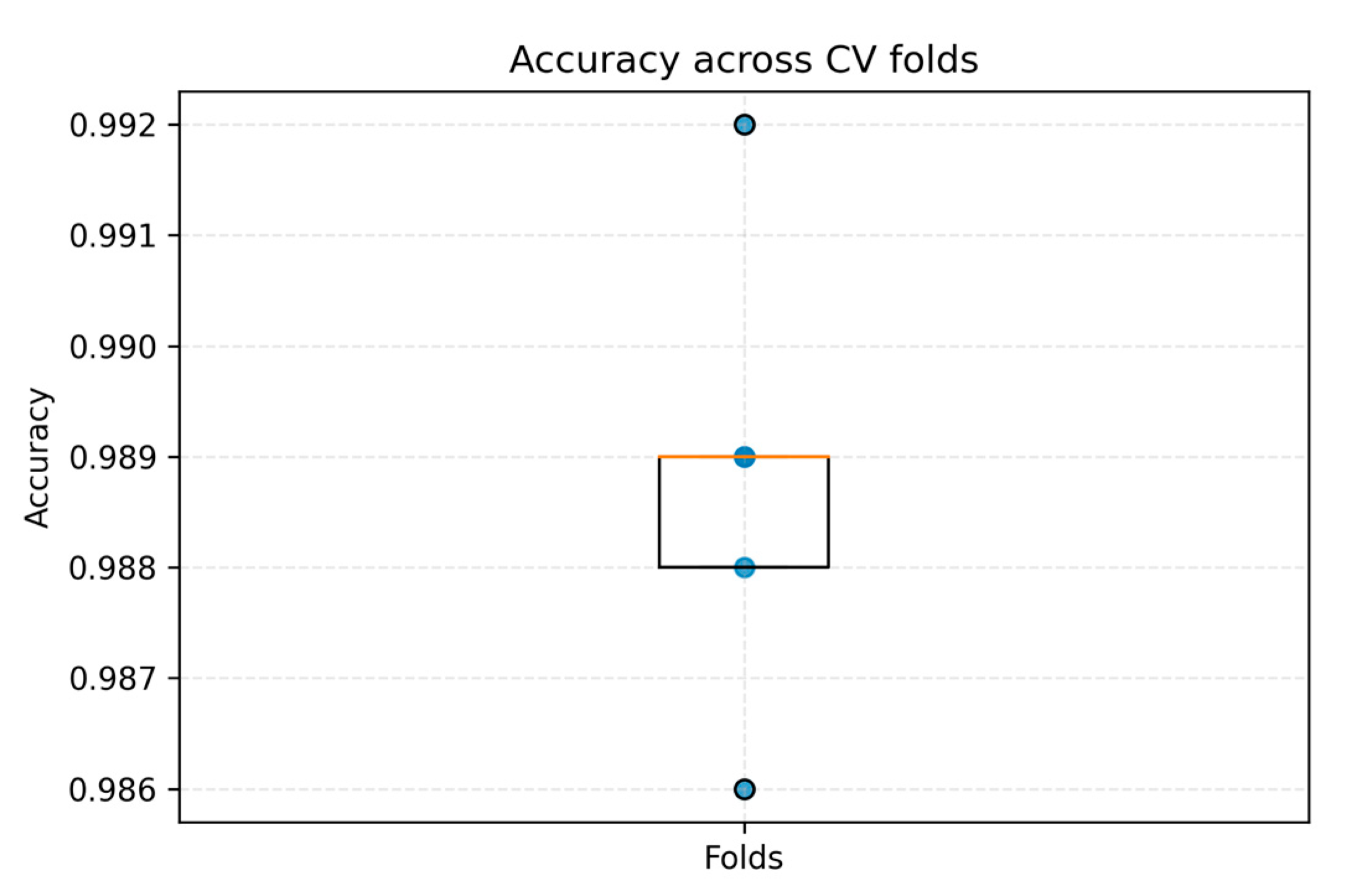
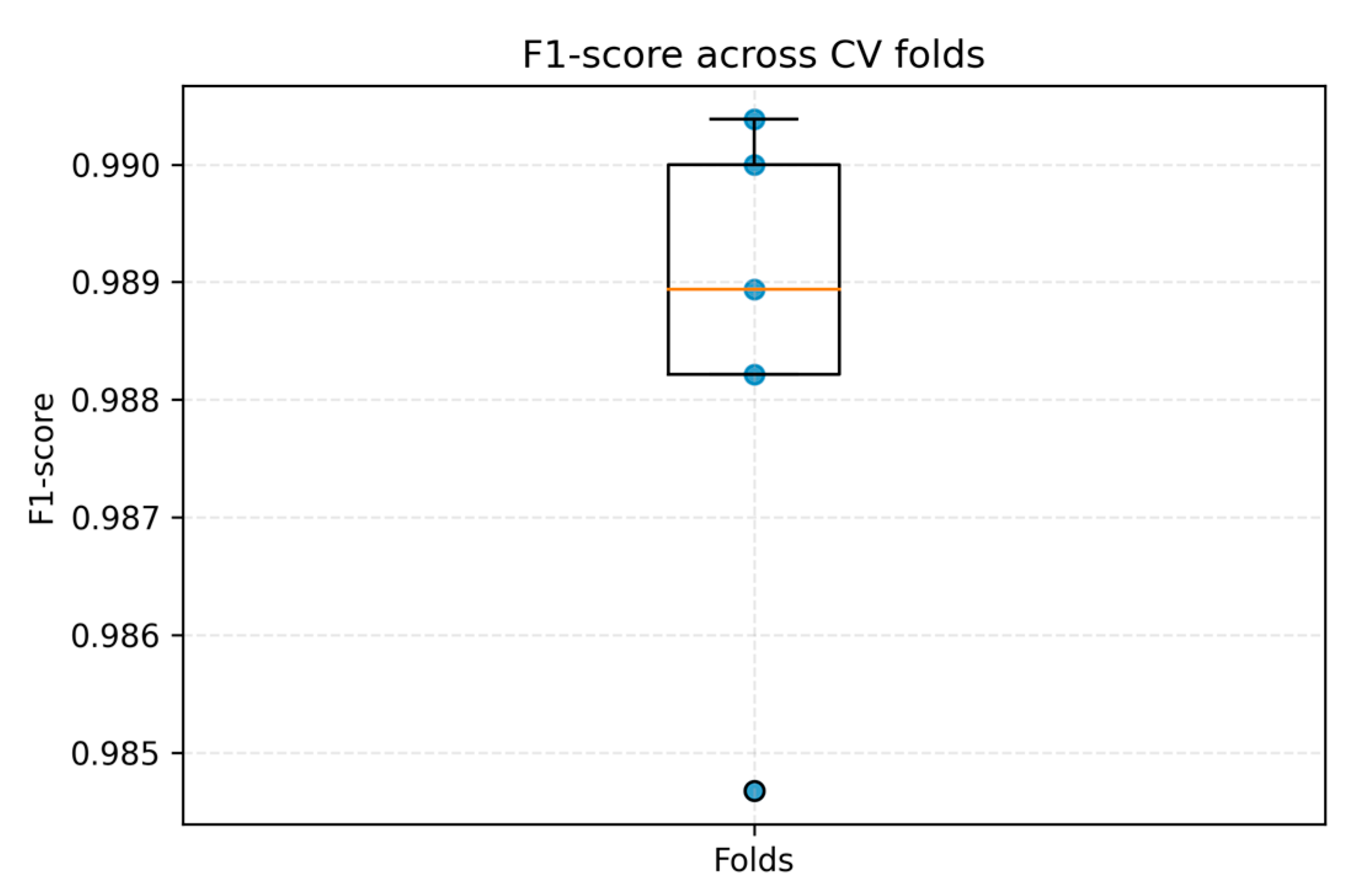
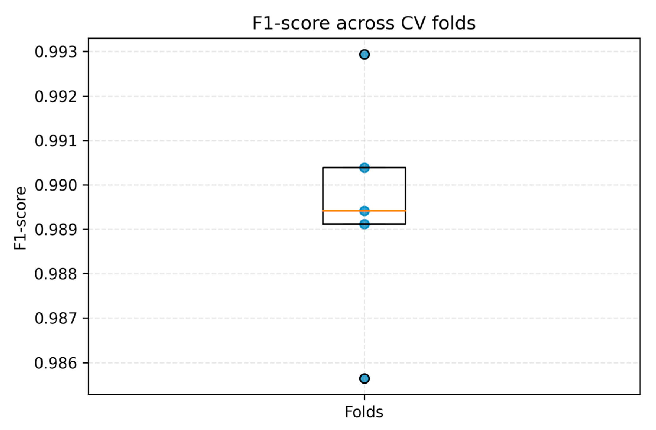
To assess the stability of the proposed framework, an additional five-fold cross-validation experiment was performed for both CNN architectures using the complete preprocessing pipeline. The same training settings were used for all folds. The average classification results are summarised in

Table 2. Five-fold cross-validation results for ResNet50 and DenseNet121.

CNN Architecture	Accuracy (%)	F1-Score (%)
ResNet50	98.76 ± 0.2074	98.8442 ± 0.2271
DenseNet121	98.88 ± 0.2168	98.9499 ± 0.2627

, while the distributions of validation accuracy and F1-score are shown in Figure 7, Figure 8, Figure 9 and Figure 10.

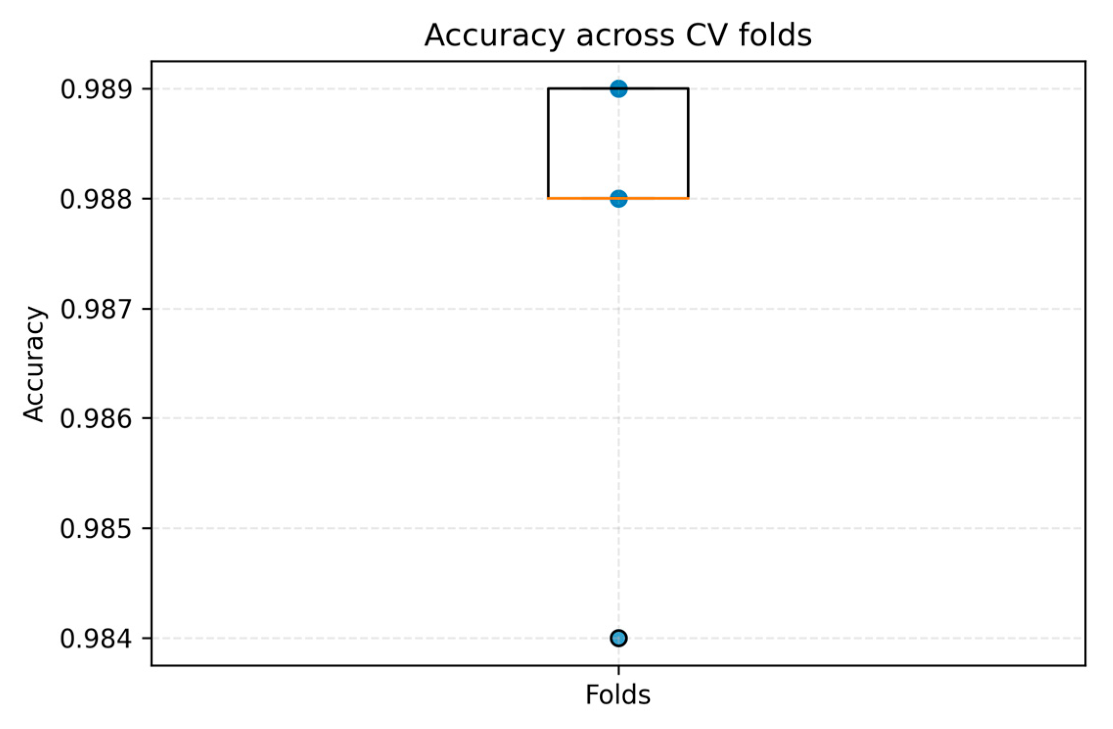
The results were similar across all five folds for both CNN architectures and validation accuracy, and F1-score showed only small variations between the individual folds, indicating stable model performance throughout the cross-validation experiments.

Figure 7, Figure 8, Figure 9 and Figure 10 illustrate the distribution of the classification metrics for each model. The relatively small spread of the boxplots indicates that the obtained results were not dominated by a particular train–validation split.

Overall, the cross-validation results show that both CNN architectures maintain stable classification performance across different data partitions.

The five-fold cross-validation produced similar results for both CNN architectures. Validation accuracy and F1-score showed only small differences between the individual folds.

Figure 7, Figure 8, Figure 9 and Figure 10 summarise the distribution of these metrics. The narrow spread of the boxplots indicates that the models performed consistently across all folds.

Overall, the cross-validation results suggest that the reported classification performance is not dependent on a particular train–validation split.

4.3. Explainability Results

The explainability performance of the investigated CNN models was evaluated using Grad-CAM, Integrated Gradients, and LIME. Localisation quality was assessed by comparing the generated explanation maps with the corresponding tumour segmentation masks using Intersection over Union (IoU), the Dice coefficient, and the Pointing Game.

The average localisation results are summarised in

Table 3. Average localisation metrics obtained from explainability maps on the validation subset.

Algorithm	Model	IoU	Dice	Pointing Game
Grad-CAM	ResNet50	13.87%	21.85%	33.33%
	DenseNet121	21.49%	30.21%	48.33%
LIME	ResNet50	7.08%	12.34%	0%
	DenseNet121	7.08%	12.34%	0%
Integrated Gradients	ResNet50	4.31%	8.23%	21.67%
	DenseNet121	2.97%	5.63%	6.67%

. Although both CNN architectures achieved high classification accuracy, the localisation metrics were considerably lower. Among the investigated explainability methods, Grad-CAM produced the highest localisation scores for both CNN models.

DenseNet121 performed slightly better than ResNet50 in the localisation analysis. It achieved an average IoU of 21.49%, a Dice coefficient of 30.21%, and a Pointing Game score of 48.33%. Grad-CAM gave the best localisation results for both models, while Integrated Gradients and LIME showed lower agreement with the annotated tumour masks.

The explanation maps were not always limited to the tumour region. In many cases, activations also appeared around the tumour boundaries or in nearby image regions, even though both CNN models classified the images correctly. This suggests that high classification accuracy does not always correspond to accurate localisation.

Localisation quality also varied between tumour types. The best results were obtained for meningioma images, while glioma and pituitary tumours generally produced more dispersed activation maps.

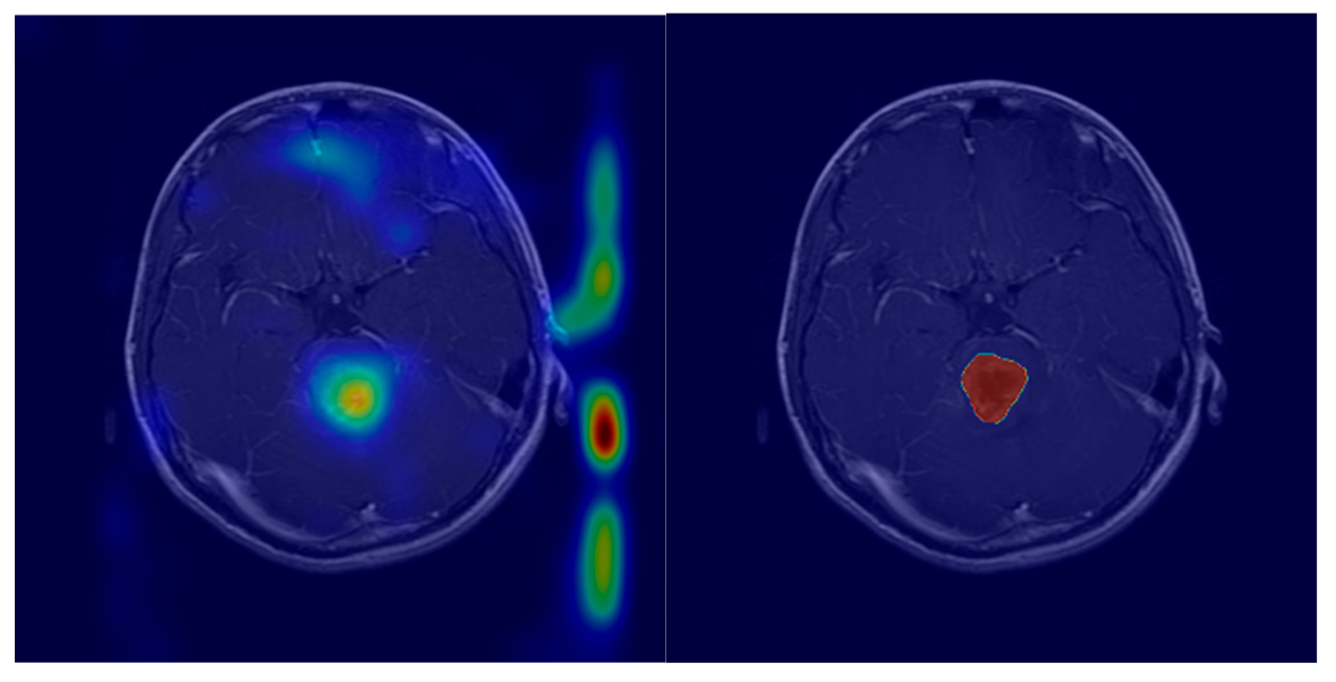
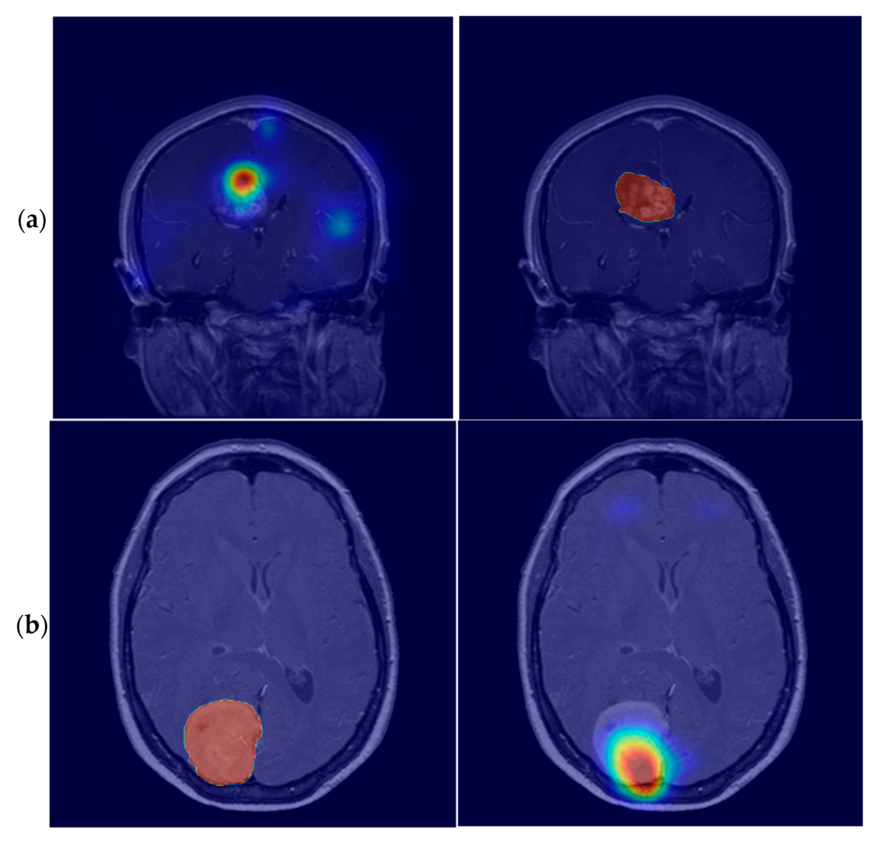
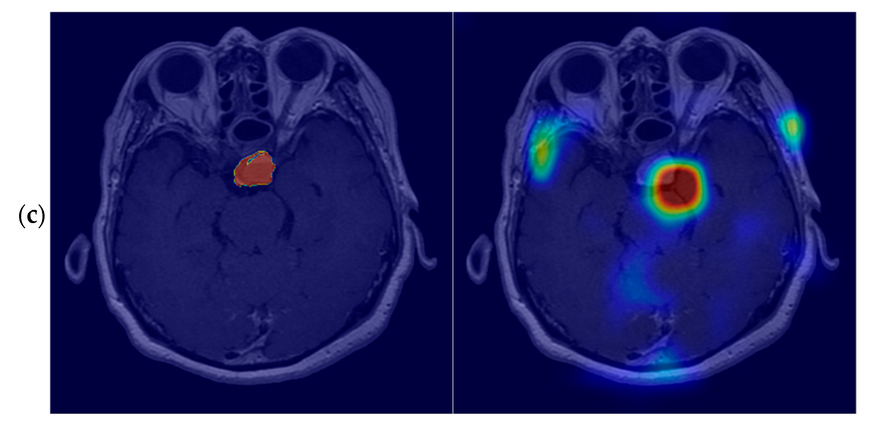
Representative Grad-CAM visualisations are presented in Figure 11. The comparison between the generated explanation maps and the corresponding tumour masks shows that the CNN models consistently identified tumour-related regions, although activations outside the annotated tumour area were still present in several examples.

These results show that classification accuracy alone is not sufficient to evaluate explainability. Quantitative localisation metrics provide additional information about how well the explanation maps correspond to the annotated tumour regions.

Among the three explainability methods, Grad-CAM consistently gave the best localisation results for both CNN models in

Table 4. Per-class explainability metrics for Grad-Cam.

Model	Class	IoU	Dice	Pointing Game
ResNet50	meningioma	29.79%	46.22%	80%
	pituitary	3%	4.85%	5%
	glioma	8.82%	14.47%	15%
DenseNet121	meningioma	46.86%	61.70%	90%
	pituitary	6.18%	10.44%	15%
	glioma	11.44%	18.49%	40%

. Integrated Gradients and LIME performed less accurately, although the difference depended on the localisation metric being considered.

The localisation results were not the same for all tumour types. Meningioma images consistently produced the best agreement between the explanation maps and the tumour masks. The highest values were obtained with DenseNet121, which reached an IoU of 46.86%, a Dice coefficient of 61.70%, and a Pointing Game score of 90%.

Glioma and pituitary tumour images proved more difficult. In these cases, the activation maps were generally less concentrated around the annotated tumour region, leading to lower localisation scores. Despite these differences, the relative performance of Grad-CAM, Integrated Gradients, and LIME remained similar across all tumour classes.

Representative examples of the generated explanation maps are shown in Figure 11 and Figure 12.

Although both CNN models achieved very high classification accuracy, the localisation quality differed considerably between the investigated explainability methods. In other words, a correctly classified image does not always produce an accurate explanation map. For this reason, classification accuracy should be considered together with quantitative localisation metrics.

4.4. Effect of Image Preprocessing

To evaluate the effect of the proposed preprocessing pipeline, both CNN models were retrained after applying Otsu thresholding, binary hole filling, and brightness–contrast jittering.

After preprocessing, Grad-CAM showed better agreement with the annotated tumour regions for both CNN architectures. In contrast, Integrated Gradients produced only minor changes in the IoU and Dice coefficient, while the Pointing Game score slightly decreased.

The average localisation results after preprocessing are presented in

Table 5. Average explainability metrics after the proposed image preprocessing steps.

Algorithm	Model	IoU	Dice	Pointing Game
Grad-CAM	ResNet50	18.27%	28.14%	43.33%
	DenseNet121	23.08%	32.49%	51.67%
Integrated Gradients	ResNet50	4.82%	9.24%	15%
	DenseNet121	3.1%	6%	5%

, whereas the corresponding per-class results are given in

Table 6. Per-class localisation metrics obtained from Grad-CAM explainability analysis after preprocessing.

Model	Class	IoU	Dice	Pointing Game
ResNet50	meningioma	30.94%	46.75%	80%
	pituitary	5.37%	8.71%	10%
	glioma	18.51%	28.96%	40%
DenseNet121	meningioma	47.83%	63.17%	95%
	pituitary	4.05%	6.97%	15%
	glioma	17.37%	27.34%	45%

.

For the DenseNet121 model, the average IoU increased from 21.49% to 23.08%, the Dice coefficient improved from 30.21% to 32.49%, and the Pointing Game score increased from 48.33% to 51.67%. Similar improvements were observed for the ResNet50 architecture. In addition, the DenseNet121 model achieved a validation accuracy of 99.6% after preprocessing.

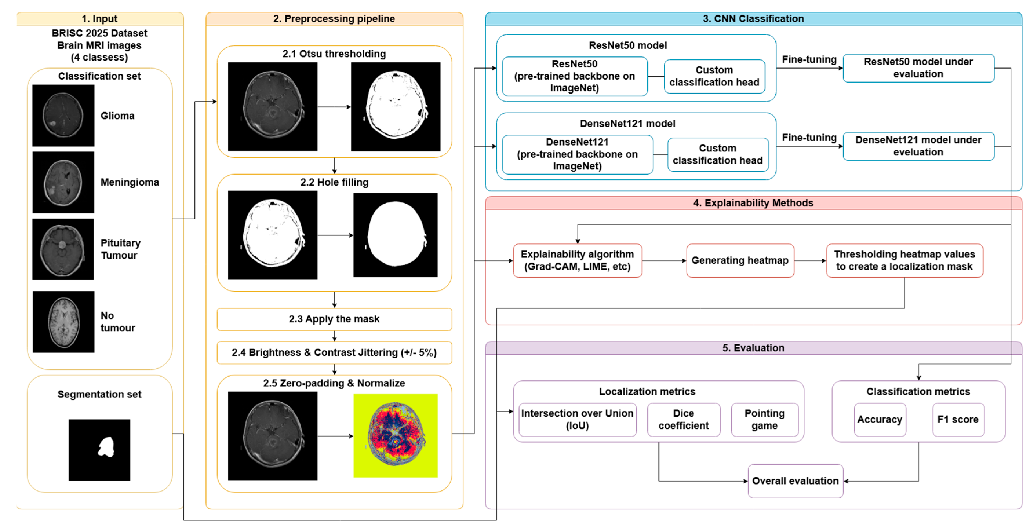
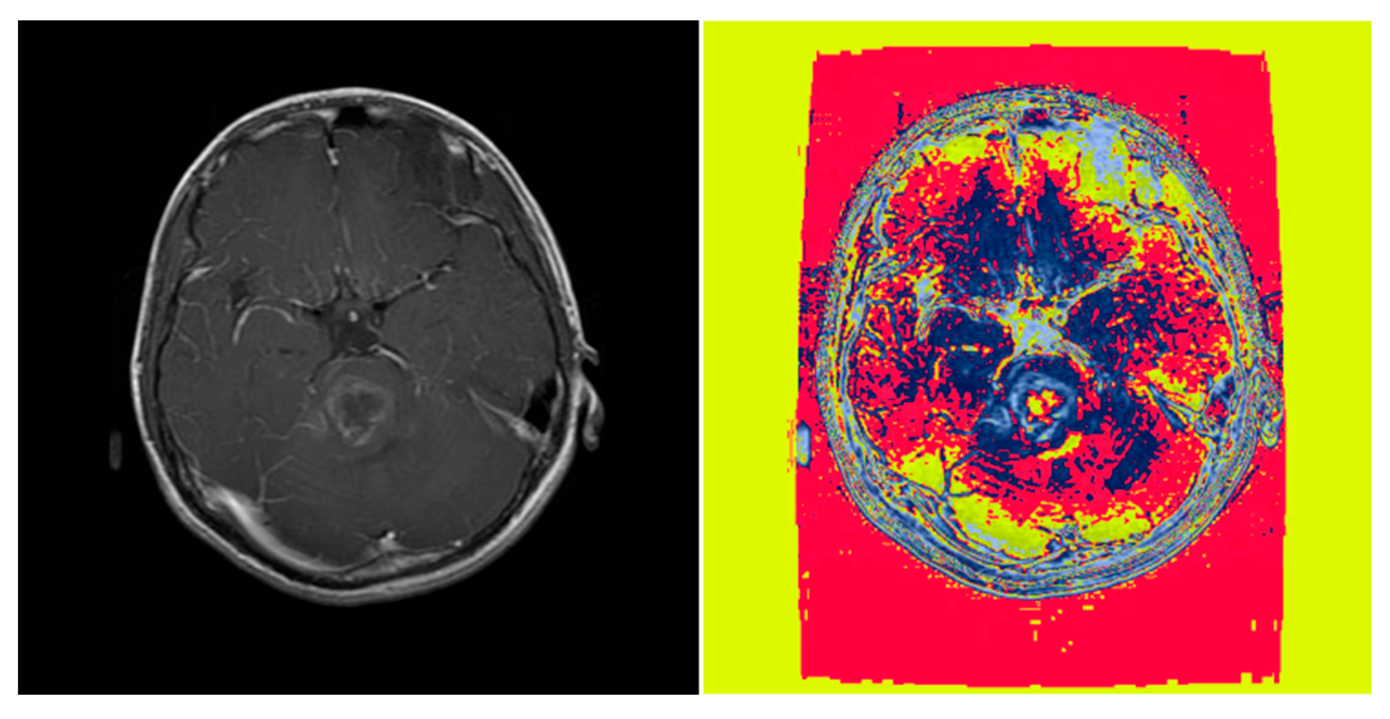
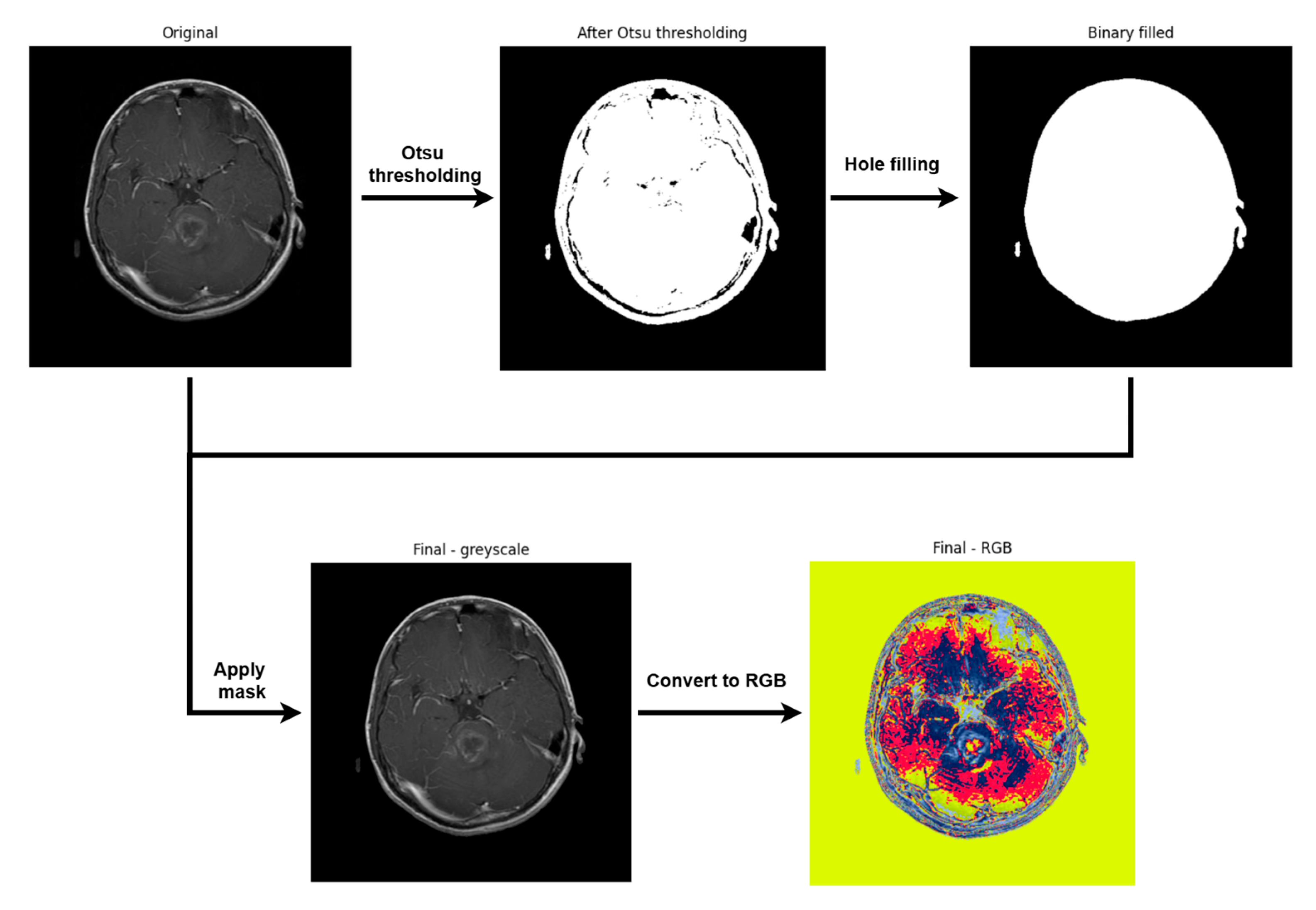
The preprocessing steps that are used in the proposed framework are shown in Figure 13, including Otsu threshold masking, binary hole filling, mask application, and RGB conversion before CNN classification and explainability analysis.

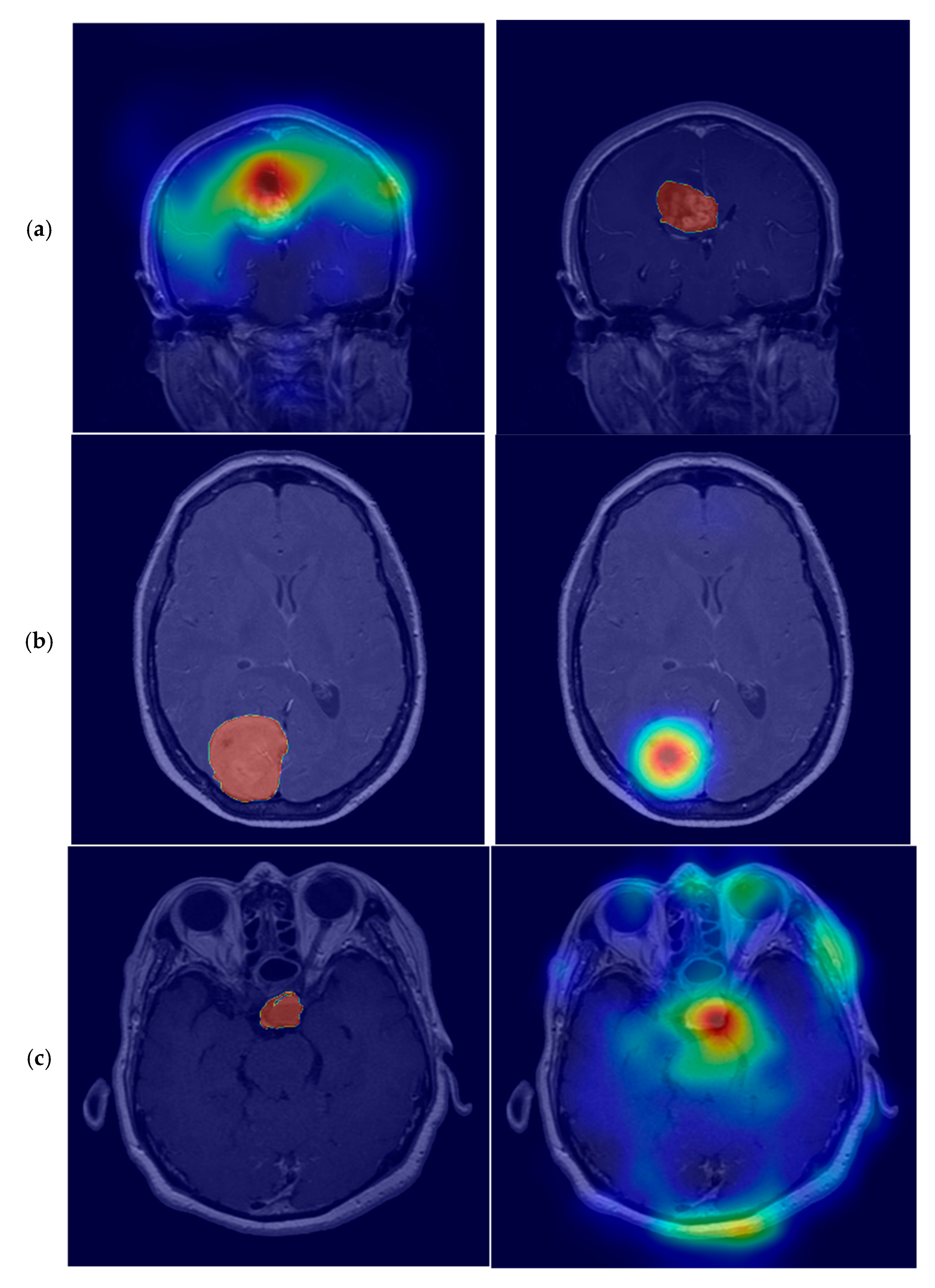
The Grad-CAM examples presented in Figure 14 and Figure 15 show fewer activations in the background and a better concentration of the highlighted regions around the tumour. This effect is particularly visible for the meningioma and glioma examples.

The preprocessing pipeline shown in Figure 13 was designed to suppress irrelevant background activations and improve localisation consistency in the subsequent Grad-CAM analysis.

An additional experiment was carried out to evaluate the contribution of each preprocessing step. Three preprocessing configurations were compared: the original MRI images, preprocessing without binary hole filling, and the complete preprocessing pipeline. The average localisation results are presented in

Table 7. Effect of preprocessing on Grad-CAM localisation metrics.

Model	Pipeline	IoU	Dice	Pointing Game
ResNet50	No preprocessing	18.99 ± 2.64%	29.69 ± 3.32%	41.99 ± 4.39%
ResNet50	Without binary hole filling	17.34 ± 1.86%	27.83 ± 2.51%	41.51 ± 4.19%
ResNet50	Full preprocessing	19.80 ± 3.04%	30.85 ± 4.38%	45.09 ± 5.84%
DenseNet121	No preprocessing	20.41 ± 0.93%	29.51 ± 1.62%	47.51 ± 6.06%
DenseNet121	Without binary hole filling	21.47 ± 1.21%	31.31 ± 1.66%	49.38 ± 4.87%
DenseNet121	Full preprocessing	22.46 ± 1.55%	32.38 ± 2.12%	51.06 ± 3.51%

.

For both CNN architectures, the complete preprocessing pipeline gave the highest Grad-CAM localisation scores. When the binary hole-filling step was omitted, all localisation metrics decreased slightly. This indicates that the hole-filling step helps preserve a more complete brain region before CNN training.

The improvements were moderate but appeared for both CNN models. Preprocessing reduced activations outside the tumour region, although localisation errors were still present. Pituitary tumour images remained the most difficult cases, with activation maps that were generally more dispersed than those observed for glioma and meningioma.

Overall, the results show that conventional preprocessing improves the localisation of Grad-CAM explanation maps, but preprocessing alone is not sufficient to eliminate all localisation errors.

The comparison between the three preprocessing configurations showed that the complete preprocessing pipeline produced the highest Grad-CAM localisation scores for both CNN architectures. Omitting the binary hole-filling step slightly reduced the IoU, Dice coefficient, and Pointing Game values, particularly for ResNet50. Although the improvements were moderate, the same trend was observed for both CNN models.

To determine whether these improvements were statistically significant, the Wilcoxon signed-rank test was applied to the localisation metrics before and after preprocessing. A significance level of p < 0.05 was used throughout the analysis. The overall results are summarised in

Table 8. Statistical significance measurement for the results from the proposed pipeline.

Model	Localisation Metric	IoU	Dice	Pointing Game
ResNet50	Grad-CAM	0.217	0.295	0.564
ResNet50	Integrated Gradients	0.498	0.422	0.405
DenseNet121	Grad-CAM	0.219	0.137	0.029
DenseNet121	Integrated Gradients	0.151	0.126	0.665

.

For Integrated Gradients, no statistically significant differences were found. This is consistent with the relatively small changes observed in the localisation metrics after preprocessing. For Grad-CAM, the analysis performed on the complete test set also did not reach statistical significance. This indicates that the overall improvement remains relatively small when all tumour classes are analysed together.

To better understand this behaviour, the statistical analysis was repeated separately for each tumour class. The corresponding results are presented in

Table 9. Per-class statistical significance measurement for the Grad-CAM results from the proposed pipeline.

Model	Class	IoU	Dice	Pointing Game
ResNet50	meningioma	0.009	0.014	0.102
ResNet50	pituitary	0.006	0.006	0.317
ResNet50	glioma	0.004	0.004	0.180
DenseNet121	meningioma	0.698	0.433	0.014
DenseNet121	pituitary	0.002	0.003	0.055
DenseNet121	glioma	0.004	0.001	0.006

. For ResNet50, statistically significant improvements were found for the IoU and Dice coefficient, whereas the Pointing Game did not reach statistical significance. For DenseNet121, the Pointing Game showed statistically significant improvement, while the IoU and Dice coefficient changed only slightly.

The largest improvements were observed for the glioma class, where all three localisation metrics increased after preprocessing. In contrast, the pituitary tumour class showed only limited improvement. In this class, the IoU and Dice coefficient remained lower after preprocessing, which explains why the statistical significance became weaker when the complete test set was analysed.

Overall, the statistical analysis indicates that the proposed preprocessing pipeline improves the localisation of Grad-CAM explanation maps. Although the improvements are moderate, they are consistent across repeated experiments and become statistically significant for several tumour classes.

5. Discussion

5.1. Classification Performance and Model Robustness

Both ResNet50 and DenseNet121 reached validation accuracies above 99% on the BRISC dataset. The additional cross-validation showed that the results changed very little from one fold to another.

DenseNet121 obtained slightly higher accuracy than ResNet50, but the difference was small. Since both models performed similarly, the explainability analysis was carried out using both architectures.

5.2. Explainability and Localisation Behaviour

The three explainability methods produced noticeably different localisation results. Grad-CAM consistently gave the best agreement with the annotated tumour regions for both CNN architectures, whereas Integrated Gradients and LIME achieved lower localisation scores. The same trend was observed in the additional cross-validation experiments.

These results show that classification accuracy alone is not enough to evaluate the reliability of CNN-based medical image classification. Although both CNN models classified most MRI images correctly, the corresponding explanation maps did not always match the annotated tumour regions. Quantitative localisation metrics, therefore, provide useful additional information when evaluating explainability methods.

5.3. Effect of Image Preprocessing

The additional experiments gave similar results for both CNN architectures. The complete preprocessing pipeline produced the best localisation scores, while removing the binary hole-filling step led to a small decrease in performance.

None of the individual preprocessing steps was sufficient on its own. The best localisation results were obtained when all preprocessing steps were used together.

The preprocessing pipeline investigated in this study is based on standard image processing techniques rather than newly developed algorithms. The main contribution of this work is the quantitative evaluation of how these preprocessing steps influence the localisation of CNN explanation maps. This makes it possible to assess the effect of preprocessing independently of changes to the network architecture.

5.4. Practical Implications

The results also show that explainability should not be judged only by visual inspection. Quantitative localisation metrics make it possible to evaluate whether the highlighted regions actually correspond to the annotated tumour.

Although the improvements after preprocessing are relatively small, they were observed for both CNN architectures. This indicates that simple preprocessing steps can improve the localisation of Grad-CAM maps without changing the CNN models or affecting their classification performance.

6. Limitations

The present study has several limitations.

First, all experiments were performed using the publicly available BRISC 2025 dataset. Although additional five-fold cross-validation, ablation experiments, and statistical analysis were carried out, validation on independent MRI datasets acquired under different imaging conditions is still needed before the proposed framework can be considered for broader clinical use.

Second, the explainability analysis was limited to Grad-CAM, Integrated Gradients, and LIME. These methods provide useful information about model behaviour, but they do not guarantee clinically correct interpretation of the underlying decision-making process. Future work will include the evaluation of additional explainability techniques and comparison with other CAM-based approaches.

Another limitation is related to the available dataset. Since the BRISC dataset contains anonymised images, patient-level independence could not be verified during the stratified cross-validation procedure. Consequently, the reported results should be interpreted within the limitations of the available data.

Finally, the explainability results were evaluated only against the provided tumour segmentation masks. They were not assessed by experienced radiologists or medical imaging specialists. Future studies will therefore include expert evaluation together with external validation using independent clinical datasets.

7. Conclusions

This study examined how conventional MRI preprocessing affects the localisation of CNN explanation maps for brain tumour classification using the BRISC 2025 dataset. ResNet50 and DenseNet121 were fine-tuned for four-class classification, while Grad-CAM, Integrated Gradients, and LIME were used to evaluate the localisation behaviour of the models.

Both CNN models reached validation accuracies above 99%, but this was only part of the picture. When the explanation maps were examined, activations were often found outside the annotated tumour regions. This shows that high classification accuracy alone is not enough to judge how reliably a model identifies the tumour.

Applying the proposed preprocessing pipeline improved the agreement between the Grad-CAM maps and the tumour segmentation masks. The largest improvements were obtained for the glioma class, whereas pituitary tumours remained the most difficult cases for localisation.

The additional cross-validation, ablation experiments, and Wilcoxon signed-rank analysis confirmed the main observations of this study. Although the overall improvements were moderate, they were observed for both CNN architectures, and statistically significant improvements were obtained for several tumour classes.

The proposed preprocessing pipeline improved the localisation of the generated explanation maps without changing the CNN models themselves. The next step will be to evaluate the approach using independent MRI datasets and compare the generated explanation maps with expert assessment by radiologists.