Rigorous Evaluation of Machine Learning Intrusion Detection for Water Treatment Systems on SWaT Network Traffic

Abstract

Intrusion detection systems (IDSs) for industrial control networks are commonly evaluated using random stratified splits, placing rows from every recorded attack in both training and test sets. Although convenient, this practice measures a model’s ability to recognise repetitions of patterns it has already seen rather than its ability to detect novel attacks. We revisit supervised and unsupervised machine-learning IDSs on the Secure Water Treatment (SWaT) dataset’s network-traffic modality, extending a prior conference study, and quantify the effect of more rigorous evaluation protocols. We evaluate five model families (XGBoost, a convolutional–MLP hybrid, a bidirectional LSTM classifier, an unsupervised LSTM-Autoencoder, and a temporal convolutional network) under three protocols: stratified random, attack-held-out, and leave-one-attack-out (LOO). Under LOO on a 30-file subsample, every supervised classifier scores below random on the majority of held-out attacks; the unsupervised LSTM-Autoencoder retains the best solo mean of 0.550 with a strongly bimodal per-attack distribution spanning 0.046 to 0.894. A sign-adjusted oracle-bound ensemble flips members whose per-attack AUROC inverts achieves a mean LOO AUROC of 0.844; adding the TCN as a fourth ensemble member does not improve the result, providing evidence that what is needed is an additional detection mode rather than another supervised classifier. We additionally report recall at a 5% false-positive-rate budget, paired Wilcoxon significance tests, and bootstrap confidence intervals. The full preprocessing, evaluation, and ensemble pipeline is released, and we argue that attack-held-out and LOO should be standard protocols for network-traffic IDS benchmarks on SWaT.

1. Introduction

1.1. Industrial Control Systems and the Attack Surface

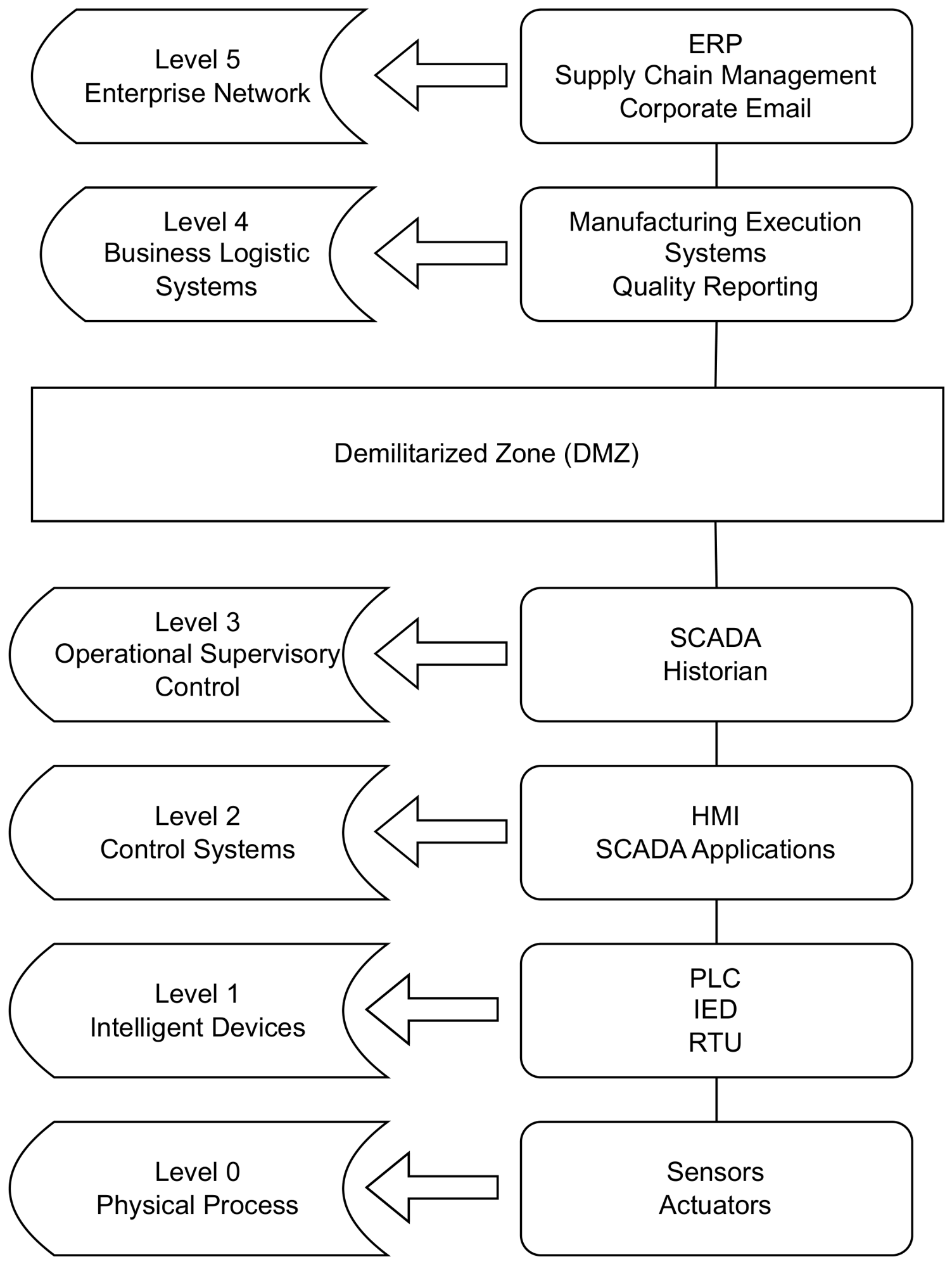
Industrial control systems (ICSs) are the digital substrate of modern critical infrastructure. They embed programmable controllers, distributed sensors, and supervisory workstations that monitor, actuate, and regulate the physical processes of electricity generation and distribution, water and wastewater treatment, oil and gas production, transportation, and discrete manufacturing [1,2,3,4]. Historically, these networks were designed in physical isolation from the corporate information-technology (IT) network, exchanging only periodic process data with enterprise systems through tightly controlled boundaries. The reference architecture for this design, the Purdue Enterprise Reference Architecture (PERA), introduced by Williams in 1993 [5], defines six hierarchical levels (Level 0 sensors and actuators through Level 5 enterprise resource planning) separated by an operational technology (OT) and IT demilitarised zone, and it prescribes that all cross-zone traffic transit a hardened broker.

The current generation of ICS deployments has eroded much of this isolation. The introduction of Industrial Internet of Things (IIoT) components, the migration of historian and analytics workloads to cloud platforms, the use of remote-access tools for vendor maintenance, and the gradual integration of OT data into enterprise resource planning have all increased the number of accessible network paths into the OT zone [1,3,6]. Field surveys consistently report that the as-deployed network topology in real plants diverges from the Purdue prescription: critical equipment routinely exposes itself to the Level 3.5 demilitarised zone or, in some cases, to the Internet, often without authentication [7,8]. The European Union Agency for Cybersecurity (ENISA) has classified ICS as a top-five threat category in its 2023 threat-landscape report, citing both nation-state and ransomware actors as principal adversaries [7].

1.2. Documented Cyber-Physical Incidents

A series of well-documented incidents establishes the practical impact of ICS intrusions: the Maroochy Shire wastewater release of 2000 [9]; the Stuxnet attack that physically destroyed approximately one fifth of the Natanz uranium-enrichment centrifuges [10]; the 2014 German-steel-mill intrusion that prevented the safe shutdown of a blast furnace [11]; the BlackEnergy 3 (2015) and CRASHOVERRIDE/Industroyer (2016) attacks on the Ukrainian power grid [12,13]; the TRISIS/TRITON malware against a Saudi Arabian Safety Instrumented System in 2017 [14]; and the Colonial Pipeline ransomware incident of 2021 [15], which halted fuel distribution to the eastern United States even though the ICS itself was not the direct target. These incidents collectively span the destruction of physical equipment, regional service outages, and supply-chain disruption.

Water and wastewater utilities specifically have been targets of recent, publicly confirmed attacks. In February 2021, an operator at the drinking-water treatment plant in Oldsmar, Florida, observed a remote session manipulating the sodium-hydroxide (lye) setpoint from 100 ppm to $11,100$ ppm via dormant desktop-sharing software, which was an event subsequently reported by the U.S. Cybersecurity and Infrastructure Security Agency [16] (Subsequent investigation has raised doubts about whether this was an external breach or an internal operator action; we cite it for the attack model it illustrates). In November 2023, the IRGC-affiliated Cyber Av3ngers group compromised a Unitronics PLC at the Municipal Water Authority of Aliquippa, Pennsylvania, prompting a joint CISA/FBI/NSA/EPA/INCD advisory [17]. The U.S. EPA has since issued sector-specific cybersecurity guidance [18], and in 2024, CISA, the FBI and EPA jointly advised operators of immediately actionable hardening steps against a sustained campaign of intrusions attributed to nation-state actors [19]. Water utilities are demonstrably an active and ongoing target for both criminal and state-sponsored adversaries.

1.3. Why Machine-Learning IDS

The traffic patterns inside an ICS network are characteristically regular: a small set of supervisory workstations periodically polls a small set of PLCs over deterministic protocols (Modbus/TCP, EtherNet/IP, OPC UA, DNP3) with payloads drawn from a finite vocabulary of read-coil and write-register operations. This regularity has long motivated the application of statistical and machine-learning methods to model normal behaviour and to flag deviations [3,4,6,20,21]. Two practical constraints, however, complicate the supervised-learning approach. First, labelled attack data are scarce; real-world ICS attacks are rare, and where attack labels exist, they are typically derived from controlled testbed exercises rather than wild incidents [21]. Second, the attacks that do exist are often single-event affairs: each attack is executed once with a particular signature and then never again. A classifier that learns those signatures may achieve near-perfect performance on a held-out portion of the same attack episode, but it offers no guarantee—and, as we show empirically in this paper, often actively misleads—when the next intrusion uses a previously unseen signature.

The Secure Water Treatment (SWaT) testbed, developed and maintained by the iTrust Centre at Singapore University of Technology and Design (SUTD) [22,23], has emerged as the community’s reference benchmark for ICS IDS research. SWaT provides labelled data from a fully operational scaled-down water-treatment plant under both normal operation and a published catalogue of 36 manually executed cyber-physical attacks. Two complementary modalities are available: physical-process readings from sensors and actuators sampled at one-second granularity, and captured network traffic between the SCADA workstation and the PLCs. Sister testbeds covering related processes—WADI for water distribution [24], EPIC for power grids, HAI for thermal power—have been released subsequently and have begun to enable cross-testbed studies. This paper, like the bulk of SWaT-related literature, restricts attention to SWaT alone; we treat cross-testbed evaluation as a critical follow-up direction.

1.4. Evaluation Protocols Matter More than They Appear

A substantial body of work on the SWaT physical-process modality uses chronological train/test splits: models are trained on the initial normal operation period (typically seven days) and tested on the subsequent attack period. Under this protocol, Kravchik and Shabtai [25] detect 32 of 36 SWaT attacks with an F1 of 0.921 using stage-wise 1D CNN autoencoders; MAD-GAN [26] reports an F1 of 0.77 with an LSTM-RNN GAN; the Graph Deviation Network (GDN) [27] further raises this to an F1 of 0.81 with a precision of 0.99 by modelling inter-sensor relationships. These numbers are achieved with rigorous, unsupervised, chronological evaluation. Work using the SWaT network-traffic modality—including our own prior conference paper evaluated under a random stratified split and achieving AUC 0.884 for XGBoost—has received considerably less methodological scrutiny. Where attacks are single non-repeating events, as in SWaT, a random split places rows from every attack in both partitions and therefore measures the ability to recognise previously seen attack signatures rather than to detect novel attacks.

1.5. Contributions

In this paper, we extend the line of rigorous evaluation on SWaT to its network-traffic modality and make the following specific contributions.

• A unified, reproducible preprocessing pipeline for SWaT network logs with content-addressed caching, an explicit handling of both date formats present in the corpus, and per-file attack-identifier annotation for downstream evaluation protocols.
• Two stricter evaluation protocols implemented as first-class code paths: attack-held-out, which guarantees that all rows of each held-out attack event are absent from training and validation; and leave-one-attack-out (LOO) cross-validation over all attack identifiers present in the sample.
• Quantification of the evaluation-protocol gap on network data: under attack-held-out, the supervised XGBoost classifier drops from an AUROC of $0.884$ under a random stratified split to a mean LOO AUROC of $0.315$ ($\sigma =0.189$) with the per-attack AUROC below $0.5$ on the majority of held-out attacks. The decision boundary is below random for most novel attacks rather than uniformly inverted, indicating that supervised models have learnt attack-specific signatures that do not transfer across attack events.
• A per-attack detectability map from LOO: an unsupervised LSTM-Autoencoder achieves a mean LOO AUROC of $0.551$ ($\sigma =0.279$) across 16 leave-one-attack-out evaluations with the per-attack AUROC spanning $0.046$–$0.894$. This bimodal distribution separates attacks that produce large physical or protocol excursions (detected by reconstruction error) from attacks whose signature interpolates inside the learnt normal envelope (effectively undetectable by reconstruction alone).
• Operating-point reporting at fixed FPR: alongside a threshold-independent AUROC, we report recall at $5\%$ FPR on each LOO fold, giving a deployment-relevant operating point and explicit false-positive and false-negative counts at the threshold-tuned $F_1$ optimum.
• A sign-adjusted ensemble that recovers the signal from inverted members. We design and release three combination rules over per-row probabilities from XGBoost, the LSTM-Autoencoder, the Bi-LSTM, and a TCN (simple average, elementwise maximum, and a sign-adjusted average that flips members whose per-attack AUROC inverts). The three-member sign-adjusted ensemble reaches a mean LOO AUROC of 0.844 ($\sigma =0.104$) and per-attack AUROC of ≥0.7 on 14 of 16 folds—a substantial recovery from any solo model and the strongest detection result we observe under leave-one-attack-out evaluation. Adding the TCN as a fourth ensemble member does not improve any of the three rules, providing evidence that a modern supervised sequence architecture does not by itself address the unseen-attack failure mode.
• An open-source code release (https://github.com/msmi12/swat-ids) (accessed on 14 July 2026) containing the full preprocessing, splits, model zoo, training loop, and evaluation harness, supporting reproducibility and further extension.

1.6. Organisation

Section 2 reviews prior work on ICS intrusion detection, SWaT-specific approaches, and the evaluation-methodology literature. Section 3 describes the SWaT dataset, our preprocessing pipeline, and the three evaluation protocols. Section 4 presents the model architectures. Section 5 and Section 6 detail the experimental setup and results. Section 7 discusses the implications for the community, and Section 8 concludes.

2. Related Work

We organise related work in three strands: (i) intrusion detection for industrial control systems in general; (ii) prior machine-learning IDSs evaluated on the SWaT dataset, separated by data modality; and (iii) the methodological literature on IDS evaluation protocols.

2.1. Intrusion Detection for ICS

The reference architecture for discussing ICS intrusion detection is the Purdue Enterprise Reference Architecture (PERA) [5], which stratifies the network into hierarchical levels from physical sensors (Level 0) to enterprise resource planning (Level 5) with a Demilitarised Zone separating IT from OT domains; Figure 1 reproduces the canonical layout.

Detection methodologies for this stack are conventionally divided along two axes: signature-based versus anomaly-based, and host-based (HIDS) versus network-based (NIDS) [4,29,30]. Signature-based detection yields high precision on known threats at the cost of recall on novel ones; anomaly-based detection flags deviations from learnt normal behaviour but is prone to false positives. Recent surveys place machine-learning-based anomaly detection at the centre of current ICS IDS research while identifying the scarcity of labelled cyber-physical attack data and the absence of standardised evaluation protocols as open challenges [2,3,6,21]. Related domain-specific work in smart-building automation [31], power grids [8], and wastewater treatment [32,33] develops analogous detection approaches under analogous data constraints.

2.2. Machine-Learning IDS on SWaT

The SWaT dataset provides two complementary modalities that are typically exploited separately in the literature. The physical-process modality records sensor and actuator states at 1 Hz from six treatment stages [22,23]. The network-traffic modality captures the OT network logs between PLCs and SCADA, including Modbus/TCP control messages.

Physical-process modality. Most methodologically rigorous SWaT IDS work to date operates on the physical-process modality under chronological evaluation. Kravchik and Shabtai [25] train per-stage 1D CNN autoencoders on the first seven normal-operation days and evaluate detection on the final four attack days, reporting a detection of 32 of 36 attacks (attacks 4, 13, 14, and 29 consistently missed), an F1 of 0.921 for the four-layer CNN ensemble, and an AUC of 0.967 on the per-record evaluation for an eight-layer CNN. Li et al. [26] introduce MAD-GAN, which is an LSTM-RNN-based generative adversarial network whose discriminator and reconstruction residuals jointly define a DR-Score. On SWaT, this yields an F1 of 0.77 (precision 0.99, recall 0.64), using a sliding window of 30 samples. Deng and Hooi [27] propose the Graph Deviation Network (GDN), which learns a directed graph between sensors and scores deviations through a graph-attention forecaster, reaching an F1 of 0.81 with precision of 0.99 and recall of 0.68 on SWaT. These works share the protocol-chronological train/test split, unsupervised (normal-only) training, and downsampling to 10 s granularity—but they differ primarily in architecture.

Network-traffic modality. Prior work on the network-traffic modality is less standardised. Our own prior study [28] reported, on a 15-file subsample drawn randomly from the SWaT network logs, binary-classification results of XGBoost, a hybrid CNN–MLP, and logistic regression, which were all evaluated under a random stratified split with a fixed seed. The study flagged recall as the principal limitation and suggested cost-sensitive loss and dynamic threshold selection as avenues for future work. This paper revisits these choices under stricter protocols.

Positioning. This paper neither disputes nor replicates the physical-process line. Its contribution is to transport the rigorous-evaluation posture that is common in that line to the network-traffic modality—and to then probe a protocol (attack-held-out/leave-one-attack-out) that is strictly stronger than the chronological split used by Kravchik, MAD-GAN, and GDN. A chronological split leaves intact the risk that attacks overlap a boundary in the training set; holding out whole attack identifiers removes that leakage entirely.

2.3. Evaluation Methodology in IDS Research

Concerns about evaluation rigour in intrusion detection extend beyond the SWaT community. Verkerken et al. [34] evaluate four unsupervised detectors (PCA, Isolation Forest, Autoencoder, One-Class SVM) in an inter-dataset setting between CIC-IDS-2017 and CSE-CIC-IDS-2018, reporting an average accuracy drop of 25.6% and AUROC drop of 30.5% relative to intra-dataset evaluation. Hesford et al. [35] benchmark six publicly available IDSs across six network datasets (CICIDS2017, UNSW-NB15, Stratosphere IoT, Mirai, BoT-IoT, ToN-IoT) and observe F1 variations of up to 70× for a single system across datasets, concluding that no single IDS is universally best and that deployment-realistic evaluation remains the exception rather than the rule.

These strands motivate the present protocol-focused contribution to the SWaT network-modality literature. Whereas Verkerken et al. measure generalisation across datasets and Hesford et al. measure it across dataset pairings, we measure generalisation across unseen attack types within the same testbed—a distinct axis of leakage that, to our knowledge, has not been systematically reported for SWaT network traffic.

2.4. Autoencoders for ICS Anomaly Detection

Autoencoders are a recurring architecture for unsupervised anomaly detection on time-series sensor data, as exemplified on SWaT by MAD-GAN [26] and the family of stage-wise CNN-autoencoder approaches of Kravchik and Shabtai [25], and by the LSTM–encoder–decoder formulation of Malhotra et al. [36] on multivariate sensor streams more broadly. The design variants vary along three axes: (i) the temporal model of the encoder and decoder (MLP, 1D CNN, RNN/LSTM, Transformer), (ii) whether the reconstruction target is the current or future input, and (iii) how anomaly scores are thresholded. The known failure mode of LSTM autoencoders—the decoder collapsing to a mean-prediction policy during early training—is documented in our experiments in Section 6 and motivates our multi-window feature set.

2.5. Recent Directions: Transformers, Graphs, Continual Learning, and Open-Set Detection

The IDS literature in 2024–2026 has consolidated around four directions that bear directly on the methodological gaps highlighted by this paper.

Transformer-based IDS. Xi et al. [37] report a multi-scale Transformer NIDS (IDS-MTran) that fuses three parallel convolutional branches at different receptive fields and a Transformer backbone, reaching >99% accuracy on NSL-KDD, CIC-DDoS2019 and UNSW-NB15. On SWaT itself, Shang et al. [38] propose CAE-T, which is an unsupervised convolutional-autoencoding Transformer trained with an SVDD-style objective, and report roughly $+2.8\%$ F₁ and $+5\%$ AUC improvements over prior unsupervised baselines. These results show that Transformer architectures are competitive on standard benchmarks; whether their advantage survives under attack-held-out evaluation on the network-traffic modality is, to our knowledge, untested.

Graph-neural-network IDS. Beyond GDN [27], two 2025 extensions are directly relevant. Lin et al. [39] introduce PCGAT, a two-level graph-attention model that maintains separate physical-process and PLC-communication graphs and reports F₁ = 0.853 on SWaT. Zhang et al. [40] propose PdGAT-ID, which combines a periodic-feature extractor with parallel spatial and temporally lagged graph-attention layers, improving F₁ by $1.55$–$5.51\%$ on SWaT, WADI, and the Gas Pipeline dataset over the best prior method. In the IoT-flow domain, Li et al. [41] extend E-GraphSAGE with an edge-enhanced multi-hop aggregator with consistent F₁ gains over E-GraphSAGE, NF-GNN, and Anomal-E on ToN-IoT and BoT-IoT. None of these works evaluate their models under a strict attack-held-out or LOO protocol on the network-traffic modality, leaving the per-attack generalisation behaviour of graph-relational IDSs an open question that the protocol introduced here could readily probe.

Continual learning IDS. Both Zhang et al. [42] (INFOCOM 2025) and Guo et al. [43] (Future Internet 2025) address the catastrophic-forgetting problem in IDS under concept drift. Zhang et al.’s SSF combines a strategic sample-selection policy with a complementary forgetting policy to keep replay-buffer memory constant; Guo et al. use clustering-based memory plus multi-level knowledge distillation between successive task models. Both report improvements over EWC and LwF baselines in class-incremental NIDS protocols. Continual learning is the natural deployment-time counterpart to our offline LOO evaluation and is named as a planned follow-up in Section 8.

Zero-day and open-set IDS. Open-set recognition explicitly targets the unseen-attack regime that LOO evaluates. Fang and Xie [44] combine Info-GAN unsupervised feature learning with an OpenMax head for novelty rejection on CIC-IDS2017. Yu et al. [45] introduce a Bi-GRU + prototype-learning open-set detector specifically for industrial networks with joint training shown to drive the gains. Qiu et al. [46] (ICTC 2024) stack OpenMax and a variational autoencoder so that two independent novelty-rejection mechanisms vote on the unknown class. These methods estimate per-fold “unknown” assignment from training-time signal alone, which is precisely the deployable approximation that our sign-adjusted ensemble called for in Section 6.3.

Cross-dataset generalisation. Two recent works complement Verkerken et al. [34] and Hesford et al. [35]. Cantone et al. [47] (IEEE Access 2024) systematically evaluate transfer between NSL-KDD, UNSW-NB15, CIC-IDS2017, and CIC-IDS2018, finding near-perfect in-distribution accuracy but near-random cross-dataset transfer, which was traced to dataset-specific feature distributions. Guo et al. [48] attack the same problem from a knowledge-injection angle: their KnowML pipeline uses LLM-distilled attack knowledge graphs to guide downstream ML-NIDS feature and model selection, reporting up to $99\%$ F₁ at FPR $<0.1\%$ on unseen attack variants where baselines collapse to F₁ = 0%. These results frame this paper’s LOO contribution as one cell of a larger evaluation landscape that is now an active research front.

3. Dataset and Methodology

3.1. The SWaT Testbed and Network Logs

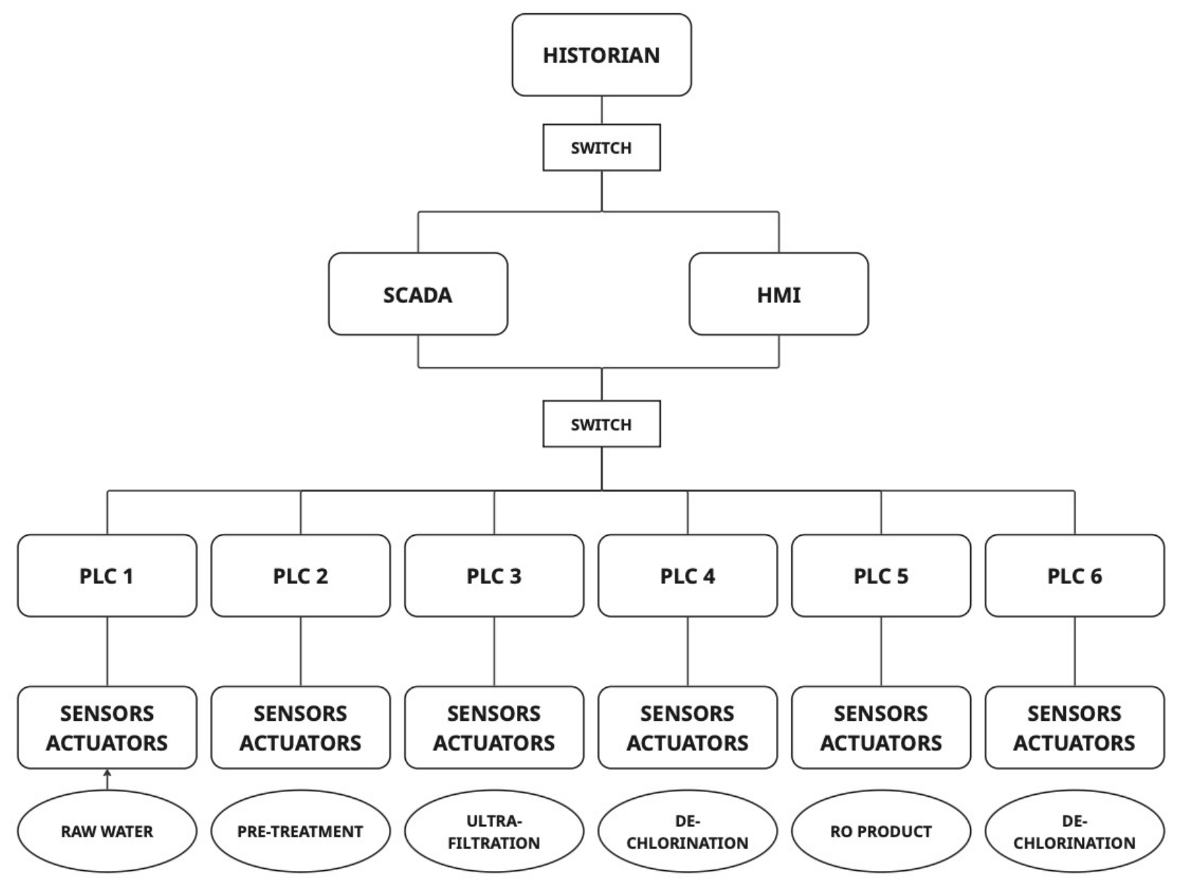
The Secure Water Treatment (SWaT) testbed, developed and maintained by the iTrust Centre for Research in Cyber Security at Singapore University of Technology and Design [22,23], is a scaled operational water-treatment plant designed for ICS security research. The plant implements a sequential six-stage purification process: raw-water intake (P1), chemical pretreatment (P2), ultrafiltration (P3), UV dechlorination (P4), reverse osmosis (P5), and permeate storage and backwash (P6). Each stage is governed by a dedicated Programmable Logic Controller (PLC) with Human–Machine Interfaces (HMIs) providing operator supervision and a central Supervisory Control and Data Acquisition (SCADA) workstation connected to a Historian for data logging. Level 1 communication follows a star topology between the SCADA workstation and the six stage PLCs; Level 0 consists of ring networks linking PLCs to their sensors and actuators. Figure 2 reproduces the testbed layout.

The SWaT dataset was generated over 11 days of continuous 24/7 operation. The first seven days capture normal operation from an empty plant state through to steady state; the remaining four days superimpose 36 predefined, manually executed cyber-physical attacks against various sensors and actuators. Two primary data modalities are recorded. The physical-process modality provides sensor and actuator readings logged by the Historian at one-second granularity (51 variables). The network-traffic modality captures the packet-level communications between the SCADA workstation and the PLCs, preserving Modbus/TCP function codes, transaction identifiers, endpoint addresses, and timing metadata. In both modalities, the binary column Tag provides the ground-truth label: 0 for normal, 1 for attack.

Scope of this paper: we focus exclusively on the network-traffic modality. This choice is motivated by two considerations. First, most prior rigorous SWaT IDS work evaluates the physical-process modality [25,26,27], leaving the network-traffic modality comparatively understudied. Second, network traffic captures the attack vector (the malicious commands traversing the OT network) in contrast to the attack effect (the anomalous physical behaviour induced by those commands). A detector that operates at the network layer can, in principle, raise an alarm before physical consequences materialise.

3.2. Preprocessing Pipeline

Our preprocessing pipeline, summarised in Figure 3, transforms the raw network logs into a per-file Parquet feature store suitable for downstream model training and evaluation. The pipeline is content-addressed: each preprocessing configuration yields a short hash (md5 over the serialised configuration) that names the output directory so that two experiments with identical preprocessing reuse a single cache.

Diverse file selection: the selection strategy greedily picks one file per distinct attack_id before filling the remaining budget with additional attack-containing files; normal-only files are sampled uniformly. With a budget of $N_a$ attack files plus $N_n$ normal files (e.g., $N_a=7$, $N_n=8$ for a 15-file sample matching the conference study, or $N_a=18$, $N_n=12$ for a 30-file sample), the procedure guarantees maximum attack-type coverage given the budget.

Feature engineering. Each selected file is streamed in 100,000-row chunks. The raw columns fall into three groups:

• Base numerical (four variables): Modbus_Function_Code, Modbus_Transaction_ID, service, s_port;
• Time-derived (five variables, engineered from date + time): cyclical encodings of hour and day-of-week as $(\sin ,\cos )$ pairs, and $\Delta t$ between consecutive records;
• Rolling statistics over service and s_port. For each window size $w\in W$ with $W\in \left\{\right\{5\},\{5,30,100\left\}\right\}$, we compute the rolling mean and rolling standard deviation strictly within each source file and strictly causally, using the pandas rolling(w, min_periods = 1) aggregation: the rolling value at row t is computed from rows $[t-w+1,t]\cap \mathrm{same}\mathrm{file}$. No future row is ever consulted, and no rolling window ever crosses a source-file boundary, eliminating the rolling-window temporal-leakage risk. The window sizes $\{5,30,100\}$ were chosen on operational rationale rather than via tuning on test data: $w=5$ captures the immediate Modbus poll-response burst, $w=30$ captures roughly half a typical SCADA polling cycle on this testbed, and $w=100$ captures a multi-cycle context that smooths over single-cycle noise. We deliberately did not perform a held-out-data sensitivity sweep on the choice of W (which would itself be a form of test-set leakage on a small sample).

All numerical features are scaled with StandardScaler, whose statistics (per-column mean and standard deviation) are fit in a streaming partial_fit pass across all selected files (not only a subset, correcting a shortcut present in [28]). We note that the scaler is fitted on the union of all selected files before the train/validation/test split is computed, so the scaler’s mean and standard deviation incorporate rows that subsequently become validation or test partitions. This is a known but limited form of preprocessing leakage: the scaler statistics are univariate and are dominated by the ≥70% normal-traffic rows that are present in every partition, so we expect the practical impact on per-fold AUROC to be small. A leakage-aware variant that re-fits the scaler on each LOO fold’s training partition is part of the streaming-loader future-work item discussed in Section 8. The remaining twelve categorical columns (orig, type, i/f_name, i/f_dir, src, dst, proto, appi_name, proxy_src_ip, Modbus_Function_Description, SCADA_Tag, Modbus_Value) are encoded via the hashing trick [21], each yielding a 32-dimensional sparse embedding that is subsequently densified. Hashing is stateless, so the categorical-encoding step introduces no leakage. The final feature vector therefore has dimension

$$d=\underset{\mathrm{base}}{\underbrace{4}}+\underset{\mathrm{time}}{\underbrace{5}}+\underset{\mathrm{rolling}}{\underbrace{2\left|W\right|}}·2+\underset{\mathrm{hashed}}{\underbrace{12·32}},$$

(1)

giving $d=397$ for single-window configurations and $d=405$ for multi-window $W=\{5,30,100\}$. Rows with NaT timestamps or invalid Tag values are dropped; each surviving row is annotated with its source filename and resolved attack_id, producing a Parquet schema of (timestamp, tag, attack_id, source_file, features…).

3.3. Evaluation Protocols

We implement three protocols as first-class code paths. Each produces a disjoint (train, validation, test) partition of the Parquet-cached rows.

Table 1. Evaluation protocols implemented in this paper. “Same-event leakage” refers to whether rows from a single attack event may appear in more than one partition.

Protocol	Same-Event Leakage	Temporal Ordering	Class Balance
Stratified random	yes	broken	balanced
Attack-held-out	no	preserved (normal)	imbalanced
Leave-one-attack-out	no	preserved (normal)	one attack/test

summarises their respective leakage properties.

Stratified random matches the protocol used in the conference paper [28] and is the de facto standard in the broader supervised-IDS literature. Rows are partitioned uniformly at random with class stratification. This protocol permits rows of the same attack event to occupy both training and test partitions, and it is reported here only as a reproduction baseline.

Attack-held-out. The unique attack_id values present in the sample (15 for our 15-file sample; 17 for the 30-file sample) are assigned disjointly: $n_{\mathrm{val}}$ attacks to validation, $n_{\mathrm{test}}$ to test, the remainder to training (we use $n_{\mathrm{val}}=3$, $n_{\mathrm{test}}=4$ by default). Normal rows (those with attack_id = 0) are ordered by timestamp and split into proportional earliest–middle–latest thirds to preserve a temporal prior without interfering with class disjointness. Because each SWaT attack is a single, non-repeating event, this protocol eliminates same-event leakage entirely at the cost of concentrating class distributions in each split.

Leave-one-attack-out. For each $a\in \{a_1,\dots ,a_K\}$ where K is the number of distinct attack_id values in the sample, we construct a separate train/val/test partition in which attack a forms the test positive set (combined with the latest 15% of normal rows), while the other $K-1$ attacks are stratified-randomly split 85/15 between training and validation (combined with the remaining normal rows). The protocol therefore yields K independent training runs per model; per-attack test metrics are aggregated to produce per-attack difficulty estimates and across-attack summary statistics. LOO is strictly stronger than attack-held-out: every attack in turn acts as an unseen test, removing any bias introduced by a specific held-out choice.

Implementation remarks. All three protocols yield pandas DataFrame objects that preserve the (timestamp, tag, attack_id, source_file) metadata columns alongside the d-dimensional feature matrix. A shared adapter converts a partition to the (X, y) NumPy tensors expected by the model API described in Section 4. All splits are parametrised by a single seed for reproducibility.

4. Models

We evaluate five model families, which were deliberately chosen to span supervised and unsupervised paradigms, and flat and sequential feature representations. All models ingest the same tabular representation described in Section 3.2; sequential models additionally construct a sliding window over consecutive rows within a single source file so that each sequence is a contiguous run of network events. Per-model hyperparameters are listed in

Table 2. Model hyperparameters fixed across protocols and sample sizes. Batch sizes listed are those used in the 30-file leave-one-attack-out configuration.

Model	Key Hyperparameters	Objective	Batch
XGBoost	500 rounds, depth 6, lr 0.1, 80% subsample	logistic	-
CNN–MLP	Conv(64,32), k = 3, MLP(64,32), drop 0.25/0.5	BCE	4096
Bi-LSTM	$T=64$, 2 layers, hidden 128 bi, drop 0.3	BCE	512
LSTM-AE	$T=64$, 2 layers, hidden 64, drop 0.2, $\tau =p_{95}$	MSE	1024
Ensemble	Logistic regression, $L_2$ $C=1.0$	logistic	-

; default values are reported here and were kept fixed across protocols and sample sizes to avoid introducing a test-time tuning confound.

4.1. Gradient-Boosted Trees (XGBoost)

XGBoost [49] serves as the strong tabular baseline, matching the configuration used in our conference paper [28]. The classifier is trained with the hist tree method on the GPU with up to 500 boosting rounds, max_depth $=6$, learning_rate $=0.1$, $80\%$ row and column subsampling, and early stopping on validation AUROC with a patience of 50. When the positive class is sparse, we set scale_pos_weight $=n_{\mathrm{neg}}/n_{\mathrm{pos}}$ on the training split. No explicit sequence information is supplied; temporal context enters only through the rolling-window features computed in preprocessing.

4.2. Hybrid 1D-CNN and MLP

To preserve continuity with the conference paper, we port the hybrid CNN–MLP architecture to PyTorch 2.4.1, keeping the layer topology unchanged. The input vector $\mathbf{x}\in {\mathbb{R}}^d$ is treated as a single-channel one-dimensional signal and passed through two blocks of Conv1d–ReLU–MaxPool1d–Dropout with 64 and 32 filters, a kernel size of 3, and a dropout of $0.25$; the flattened representation is fed into a three-layer MLP ($64\to 32\to 1$) with a dropout of $0.5$ before the output unit. The model is trained with BCEWithLogitsLoss, a learning rate of ${10}^{-4}$, a batch size of 4096, and early stopping on validation AUROC with a patience of 5. Although tabular XGBoost usually outperforms this architecture on the flat representation, we retain it as a direct comparability anchor with our prior result and as evidence that the protocol gap we report in Section 6 is not an artefact of a single model family.

4.3. Bidirectional LSTM

The first of the two sequential models is a supervised bidirectional LSTM [50,51]. The network stacks two bidirectional LSTM layers with a hidden size of 128 per direction and an inter-layer dropout of $0.3$, which is followed by a linear head over the final timestep. Input sequences of length $T=64$ rows are built by a sliding window over the feature matrix; the label assigned to each sequence is the label of its final row, so the model must decide attack versus normal on the current event given its immediate past and near future. Training uses Adam with a learning rate of ${10}^{-3}$, a batch size of 512 (reduced from 1024 in preliminary runs to avoid CUDA out-of-memory on the 30-file leave-one-attack-out configuration; see Section 8), and the same AUROC-based early stopping policy. Because the Bi-LSTM consumes future context within the window, it is strictly an offline detector; we make this choice explicit rather than implicit.

4.4. LSTM Autoencoder

The second sequential model is an unsupervised LSTM autoencoder, which is motivated by the long line of reconstruction-based anomaly detectors for multivariate sensor streams [25,26,36]. The encoder is a two-layer LSTM with a hidden size of 64; the final hidden state is tiled T times and passed through a second two-layer LSTM decoder, which is followed by a linear projection back to input dimensionality. The model is trained with mean-squared-error reconstruction loss on the subset of windows in which every timestep is labelled normal, so that no attack signal leaks into the training objective. At inference time, each window receives a reconstruction MSE; we convert MSE to an anomaly probability by the logistic transform

$$p_{\mathrm{anom}}\left(\mathbf{x}\right)=\sigma \left({\displaystyle \frac{\mathrm{MSE}\left(\mathbf{x}\right)-\tau }{{\sigma }_{\mathrm{val}}}}\right),$$

(2)

where $\tau$ is the 95^th percentile of reconstruction errors on all-normal validation windows and ${\sigma }_{\mathrm{val}}$ is their standard deviation. Hyperparameters are identical to those of the Bi-LSTM except for hidden size and the 95-th-percentile threshold.

Two practical properties of this model matter for the evaluation that follows. First, because training uses no attack labels, detection quality is necessarily threshold-sensitive; we therefore report both the threshold-independent AUROC and the threshold-tuned F₁ to disentangle ranking ability from operating-point choice. Second, reconstruction scoring favours attacks that induce large physical or protocol excursions over attacks whose signature resembles a plausible continuation of the normal process, which is a bimodality we examine in Section 6.2.

4.5. Temporal Convolutional Network (TCN)

The fourth supervised model is a Temporal Convolutional Network (TCN), which is included as a representative modern-architecture sequence baseline alongside the recurrent Bi-LSTM. We choose TCN over a Transformer encoder for the same role: TCN is closer in spirit to the existing CNN-MLP and Bi-LSTM (dilated causal 1D convolutions), trains stably without architecture-specific tuning, and matches the receptive field of the Bi-LSTM ($T=64$) with deterministic memory cost. The architecture stacks five residual TCN blocks with a kernel size of 3, channel widths of 32, and dilations $\{1,2,4,8,16\}$, yielding receptive field $1+2·{\sum }_{k=0}^4{2}^k=63$. Each block applies two padded causal convolutions with ReLU activations, a dropout of $0.2$, and a 1 × 1 residual projection. The final timestep’s channel vector is passed through a linear head to produce the binary logit. Training uses Adam with a learning rate of ${10}^{-3}$, a batch size of 128, and the same early-stopping policy as the other neural models. As with the Bi-LSTM, the TCN consumes only the past $T-1$ timesteps for the current decision and is therefore deployment realistic for streaming inference (unlike the Bi-LSTM, which is offline by design).

4.6. Stacked Ensemble

The final model is a stacked ensemble [52] over the heterogeneous base learners. Concretely, each base model produces per-row attack probabilities ${\widehat{p}}_k\left(\mathbf{x}\right)$ on validation data; a logistic-regression meta-learner is fitted on the stacked vector ${({\widehat{p}}_1,\dots ,{\widehat{p}}_K)}^{\top }$ against validation labels with $L_2$ regularisation ($C=1.0$) and up to 1000 iterations. Two design considerations are worth recording explicitly.

The first is the handling of sign inversion. Under attack-held-out evaluation, a supervised base learner may invert on held-out attacks, that is, produce an AUROC reliably below $0.5$; this is not a symptom of poor learning but of the held-out attack occupying a region of feature space opposite to the training attacks along the relevant decision direction. We therefore also report a simpler ensemble rule, sign-adjusted averaging: for each held-out attack, we flip the probabilities of any member whose per-attack AUROC is below $0.5$ before averaging. This rule uses the held-out labels only to diagnose inversion, not to pick an operating point, and it is useful as an upper bound on what a meta-learner could achieve if it had attack-level labels.

The second is the choice of validation stage for the meta-learner. Under strict attack-held-out evaluation, the meta-learner must be fitted on validation predictions produced on attacks that are themselves disjoint from both the training attacks of its members and the final held-out test attack. We enforce this by forming the validation split from the training-attack portion of the data, not from a temporal tail of the held-out attack, so the ensemble never sees the test attack in any form during meta-fitting. The alternative—fitting the meta-learner on predictions for the held-out attack—would constitute the precise evaluation leakage we critique in Section 2.3.

5. Experimental Setup

5.1. Hardware and Software Stack

All experiments were run on a single NVIDIA RTX 4090 (24 GB VRAM), which was paired with a container allocation of 62 GB of system RAM. The raw SWaT A6 capture is stored in a Google Cloud Storage bucket. The preprocessing pipeline runs once and produces the content-addressed Parquet cache described in Section 3.2; the evaluation harness consumes the cache directly.

5.2. Preprocessing Configurations and Sample Sizes

We evaluate two preprocessing configurations that differ only in the rolling-window set W. The baseline configuration uses $W=\left\{5\right\}$, matching the conference paper, yielding a feature dimensionality $d=397$. The multi-window configuration uses $W=\{5,30,100\}$, capturing additional temporal granularity at the cost of $d=405$. Two sample sizes are evaluated: a 15-file sample (7 attack-containing files plus 8 normal files, matching the conference study), and a 30-file sample (18 attack-containing files plus 12 normal files), the latter chosen via the diverse-selection strategy described in Section 3.2 to maximise the number of distinct attack_id values represented in the cache. The 30-file sample contains 17 distinct attack identifiers and approximately 14.8 M rows; the 15-file sample contains 15 distinct attack identifiers and approximately 7.4 M rows.

5.3. Training Details

For every model and every protocol, we use the hyperparameters reported in Table 2; no per-protocol or per-attack tuning is performed both to keep the comparison clean and to avoid introducing a test-time tuning confound. Training employs early stopping on validation AUROC with a per-model patience: 50 boosting rounds for XGBoost (out of a maximum of 500) and 5 epochs for the neural networks (out of a maximum of 20). Class imbalance is addressed by setting scale_pos_weight to the negative-to-positive ratio for XGBoost and pos_weight to the same ratio in the binary cross-entropy loss for the supervised neural networks; the LSTM-Autoencoder is trained only on all-normal windows and therefore requires no class weighting. Random number generators are seeded (seed = 42) for the train/validation split and for the leave-one-attack-out cross-validation, so all reported runs are exactly reproducible.

5.4. Computational Cost

The per-model training time, inference latency on the $3,425,084$-row attack-held-out test partition, peak GPU memory, and serialised model size are summarised in

Table 3. Per-model training and inference cost on the 30-file multi-window cache, one attack-held-out fold. Inference latency is on the $3.4$-million-row test partition; peak VRAM is measured via torch.cuda.max_memory_allocated. The Bi-LSTM training time at batch_size $=256$ is the dominant per-fold cost; the LOO ensemble of 16 folds takes $\approx 4.5$ h wallclock for Bi-LSTM alone.

Model	Train (s)	Infer. (μs/row)	Peak VRAM (MB)	Model Size (MB)
XGBoost	23.5	1.97	–	0.34
CNN–MLP	194.9	9.13	19,156	0.83
LSTM-AE	331.6	11.00	19,063	0.94
Bi-LSTM	608.3	15.98	18,404	3.60
TCN	563.8	12.85	18,165	0.31

. All measurements are on a single fold of the 30-file multi-window cache in the hardware listed in Appendix A. The training-time row should be read alongside the LOO compute footprint of 16 folds; the inference latency row is the deployment-relevant figure—even the slowest base model processes more than $60,000$ rows per second, which exceeds typical SWaT network capture rates.

5.5. Evaluation Metrics

Every test-time prediction yields a per-row attack probability $\widehat{p}\in [0,1]$. From this, we compute the threshold-independent area under the receiver operating characteristic curve (AUROC) and a sweep over candidate thresholds to obtain the threshold-tuned $F_1$ score and its associated recall (denoted best-$F_1$ recall hereafter). Where the LOO test partition contains rows from a single attack only, AUROC describes the ability to rank that attack’s rows above the temporally disjoint normal rows; thus, an AUROC of $0.5$ means random ranking, an AUROC below $0.5$ means the ranker is on the wrong side of the decision (worse than random; equivalent to a flipped predictor with AUROC $1-x$ if used as-is), and an AUROC above $0.7$ is the threshold beyond which a downstream operator can plausibly find an operating point with both reasonable recall and a bounded false-positive rate.

6. Results

We report results in three layers, of increasing strictness. Section 6.1 reproduces the conference-paper protocol (random stratified) on our unified pipeline as a baseline and then contrasts it with attack-held-out and leave-one-attack-out. Section 6.2 drills into the leave-one-attack-out evaluation, the most rigorous and most informative protocol, and presents the per-attack detectability map for all four trained models (XGBoost, LSTM-Autoencoder, Bi-LSTM, and TCN). Section 6.3 reports stacked-ensemble results that recover signal from the supervised models that, individually, score below random under attack-held-out evaluation.

Two orthogonal axes. Before reporting the numbers, we emphasise that the two methodological axes the paper examines—(i) supervised vs. unsupervised training, and (ii) evaluation under random stratified split vs. attack-held-out/leave-one-attack-out—are independent. Each $\mathrm{axis}\text{-}1\times \mathrm{axis}\text{-}2$ cell has a different failure mode. Supervised + random memorises within-attack signatures, scores AUROC > 0.85 (

Table 4. Test AUROC by evaluation protocol. Random: stratified-random split of rows; values reproduced from the conference paper [28] on the 15-file single-window cache and shown for context only—they are dominated by within-attack row exposure across train/test by construction. Held-out (1): single attack-held-out fold on the 30-file multi-window cache ($n_{\mathrm{val}}=3$, $n_{\mathrm{test}}=4$, seed 42). LOO (mean): averaged across the 16 leave-one-attack-out folds on the same 30-file multi-window cache. Values below $0.5$ indicate that the model ranks the held-out attack rows below the temporally disjoint normal rows—it scores below random.

Model	Random †	Held-Out (1)	LOO (Mean)
XGBoost	0.884	0.078	0.315
CNN–MLP	0.875	0.351	N/A ‡
Bi-LSTM	–	0.180	0.215
LSTM-AE	–	0.730	0.550

^† Random-split values reproduced from the conference paper [28] on the 15-file sample with rolling window $W=\left\{5\right\}$; we did not re-run random-split evaluation on the 30-file multi-window cache because under the random protocol attack, rows are already exposed during validation, and the resulting AUROC is a known artefact (Section 2.3). The other three columns are computed on the 30-file multi-window cache (11a8c45b6157); “Held-out (1)” is a single attack-held-out fold with $n_{\mathrm{val}}=3$, $n_{\mathrm{test}}=4$, seed 42; “LOO (mean)” averages across the 16 folds ^‡ The CNN–MLP was not included in the LOO sweep; under the single attack-held-out fold, it patterns with the other two supervised models.

), gives no guarantee on novel attacks. Supervised + attack-held-out scores below-random on the held-out attacks whose signatures are absent from training (XGBoost LOO mean $0.315$, Section 6.2). Unsupervised + random catches deviations from reconstructed-normal regardless of attack identity, but the random split inflates apparent precision by exposing within-attack rows to validation thresholds. Unsupervised + attack-held-out detects out-of-envelope attacks (LSTM-AE on attacks 23/25/26/28/29) and misses in-envelope attacks (LSTM-AE on attacks 19/20).

6.1. Protocol Comparison

Table 4 summarises the mean test AUROC for each (model, protocol) combination on the 30-file sample. Three observations are immediate.

First, the random-split column is consistent with the high AUROC values reported across the SWaT network-traffic literature (XGBoost $0.884$, CNN–MLP $0.875$), which under that protocol partly reflect repeated exposure to within-attack rows in both training and test. Second, the attack-held-out column on a single 4-attack test partition drops every supervised model to AUROC below random, suggesting that the supervised models have learnt attack-specific signatures that not only fail to transfer but actively mislead on at least the held-out attacks in this partition. Third, the LOO mean over 16 distinct held-out attacks confirms that this is not an artefact of one unfortunate attack choice: XGBoost’s LOO mean of $0.315$ aggregates across attacks whose individual AUROC ranges from $0.093$ to $0.690$ (Section 6.2) with 12 of 16 folds at AUROC values below $0.5$; the LSTM-Autoencoder’s LOO mean of $0.551$ similarly spans $0.046$ to $0.894$ with 7 of 16 folds above $0.7$ and three below $0.1$.

The gap between the random column and the LOO column—on the order of $0.5$ AUROC for XGBoost—quantifies the cost of evaluating ICS network IDS under leakage-prone protocols. To our knowledge, no prior work on the SWaT network modality has reported this gap.

6.2. Leave-One-Attack-Out Analysis

The leave-one-attack-out cross-validation removes the dependence of summary statistics on a particular held-out choice.

Table 5. Per-attack composition of each LOO test partition on the 30-file multi-window cache. Imbalance is $n_{\mathrm{normal}}:n_{\mathrm{positive}}$. Attack 14, with $n_{\mathrm{positive}}=4$, is excluded from the LOO summary statistics (Section 6.2).

Atk ID	${\mathit{n}}_{\mathbf{test}}$	${\mathit{n}}_{\mathbf{attack}}$	${\mathit{n}}_{\mathbf{normal}}$	Imb.
1	1,873,890	220,512	1,653,378	$1:7.5$
8	2,006,495	353,117	1,653,378	$1:4.7$
14 †	1,773,347	4	1,773,343	$1:>{10}^5$
15	1,811,448	158,070	1,653,378	$1:10.5$
16	1,754,564	101,185	1,653,379	$1:16.3$
19	1,748,159	94,780	1,653,379	$1:17.4$
20	1,798,193	144,815	1,653,378	$1:11.4$
21	1,771,488	118,100	1,653,388	$1:14.0$
23	1,908,484	255,106	1,653,378	$1:6.5$
25	1,877,799	224,421	1,653,378	$1:7.4$
26	1,672,599	19,221	1,653,378	$1:86.0$
27	1,725,114	52,673	1,672,441	$1:31.8$
28	3,093,540	1,440,162	1,653,378	$1:1.1$
29	1,697,883	44,505	1,653,378	$1:37.2$
30	1,807,142	153,752	1,653,390	$1:10.8$
33	1,816,064	162,679	1,653,385	$1:10.2$
35	1,768,383	115,005	1,653,378	$1:14.4$
Sum16	30,131,245	3,658,103	26,473,142	–

^† Excluded from $n=16$ LOO summary statistics; see prose.

first reports the composition of each LOO test partition: every fold’s test set consists of all rows of the held-out attack joined with the temporally last $15\%$ of normal rows (≈1.65 million rows). The class imbalance varies substantially across folds because the attacks themselves differ in duration; attack 28 produces $1,440,162$ attack rows (a $1:1.1$ ratio with normal rows) while attack 26 produces only $19,221$ ($1:86$). Attack 14, whose temporal-tail test partition contains only $four$ attack rows, with the AUROC estimate at $n_{\mathrm{positive}}=4$ is dominated by per-row label noise, and including it inflates the LSTM-Autoencoder mean from $0.550$ to $0.576$ without scientific information gain. We therefore restrict the LOO summary in

Table 6. Per-attack test AUROC under leave-one-attack-out evaluation on the 30-file multi-window sample. Each row holds out one of the 16 attack identifiers with $n_{\mathrm{positive}}\ge 19,000$ (see Table 5; attack 14 has $n_{\mathrm{positive}}=4$ and is excluded as noted in Section 6.2). The TCN column reports the dilated causal 1D convolutional model introduced as the modern-architecture baseline in Section 4.5. Bold entries exceed $0.7$. The rightmost column reports the sign-adjusted-average ensemble of the four base models; it consults held-out labels to determine direction and is therefore an oracle bound rather than a deployable detector.

Atk ID	XGBoost	LSTM-AE	Bi-LSTM	TCN	Sign-Adj. Ensemble
1	0.200	0.310	0.145	0.175	0.933
8	0.147	0.725	0.300	0.123	0.924
15	0.340	0.825	0.015	0.221	0.735
16	0.318	0.373	0.128	0.232	0.789
19	0.690	0.062	0.503	0.423	0.611
20	0.561	0.046	0.409	0.564	0.572
21	0.682	0.511	0.341	0.248	0.943
23	0.175	0.841	0.080	0.127	0.955
25	0.171	0.852	0.078	0.107	0.960
26	0.203	0.873	0.248	0.302	0.959
27	0.203	0.397	0.087	0.239	0.917
28	0.093	0.835	0.135	0.322	0.953
29	0.533	0.894	0.149	0.368	0.836
30	0.263	0.456	0.239	0.294	0.756
33	0.143	0.391	0.173	0.332	0.824
35	0.320	0.415	0.417	0.373	0.780
Mean	0.315	0.550	0.215	0.278	0.840
$\sigma$	0.189	0.279	0.138	0.117	0.121

,

Table 7. Mean operating-point statistics across the 16 LOO folds at the threshold that maximises $F_1$ on each fold. R_5% is the recall achievable while holding the false-positive rate at ≤5%.

Model	Mean ${\mathit{F}}_1$	Mean R5%	Mean FN
XGBoost	0.209	0.000	4789
LSTM-AE	0.264	0.073	16,492
Bi-LSTM	0.180	0.000	1580

and

Table 8. Mean LOO AUROC across the 16 folds for each base model in isolation and for each ensemble combination rule. The 3-member ensembles combine XGBoost, LSTM-AE, and Bi-LSTM; the 4-member ensembles add TCN. The sign-adjusted average is bold-faced because it is the headline ranking-quality figure, but it is an oracle bound (uses held-out labels to determine direction; see prose).

Combination Rule	Mean LOO AUROC	$\mathit{\sigma }$
Solo
XGBoost	0.315	0.189
LSTM-AE	0.550	0.279
Bi-LSTM	0.215	0.138
TCN	0.278	0.117
Ensemble of three base members (XGBoost, LSTM-AE, Bi-LSTM)
Simple average	0.278	0.165
Maximum (OR rule)	0.333	0.145
Sign-adjusted average	0.844	0.104
Ensemble of four base members (TCN added)
Simple average	0.245	0.132
Maximum (OR rule)	0.307	0.125
Sign-adjusted average	0.840	0.121

to the 16 folds with $n_{\mathrm{positive}}\ge 19,000$.

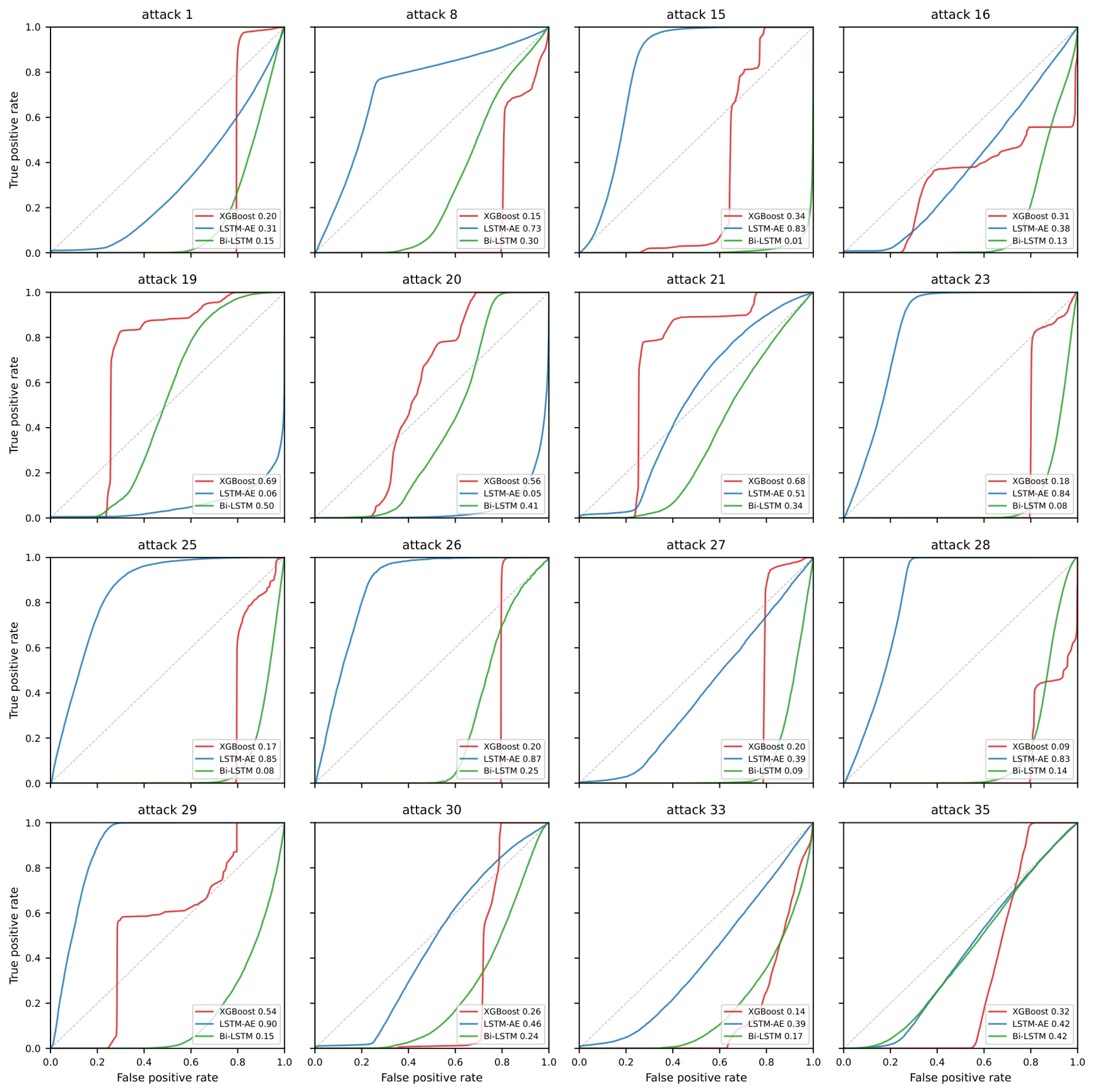
Table 6 and Figure 4 report the per-attack test AUROC and associated ROC curves for each of the four trained models (XGBoost, LSTM-Autoencoder, Bi-LSTM, and TCN) on the same 30-file multi-window sample; values shown in bold exceed $0.7$ (a heuristic threshold for plausible deployability).

Operating-point statistics are summarised in Table 7. At the threshold that maximises $F_1$ on each fold, the false-negative and false-positive counts are both large for every solo model, reflecting that AUROC values well below $0.7$ admit no operating point with simultaneously high recall and bounded false-positive rate. Recall at a fixed false-positive rate of $5\%$ (R_5%) is essentially zero across all three solo models on every fold; deployment-relevant detection on SWaT network traffic under unseen-attack evaluation requires the ensemble combination of Section 6.3.

The pattern visible in Table 6 is striking and is the central empirical contribution of this paper. The two model families exhibit opposite sets of detectable attacks. The XGBoost classifier achieves above-chance performance only on attacks 19, 20, 21 and 29; on every other held-out attack, it ranks the attack rows below the normal rows—the sign of a model whose decision boundary, learnt from other training attacks, lies on the wrong side of the held-out attack’s signature. The LSTM-Autoencoder displays the converse pattern: it detects attacks 8, 15, 23, 25, 26, 28 and 29 with AUROC values of $0.7$ or higher (and $0.8$ or higher for five of them), but it is no better than chance, or actively misses, on attacks 19, 20 and 27.

This bimodality has a clean physical interpretation that we elaborate on in Section 7. Attacks that induce large excursions in sensor readings or actuator commands—visibly outside the autoencoder’s learnt envelope of normal behaviour—are detected by reconstruction error regardless of whether their identity was seen during training. Attacks that closely mimic the statistical envelope of normal operation (e.g., sensor-spoofing attacks 19 and 20, where the malicious commands deliberately interpolate inside the normal range) cannot be flagged by reconstruction alone.

The supervised XGBoost succeeds on a different subset (19, 20, 21, 29) because for those attacks, the discriminative features useful within the training set happen also to be useful for the held-out attack; for the rest, the feature regions occupied by the held-out attack do not coincide with those of any training attack. Under the LSTM-Autoencoder’s much weaker assumption (“attack rows are unlike anything I saw during normal-only training”), the per-attack distribution of detectability is simply that of attacks-as-physical-events rather than attacks-as-similar-to-other-attacks.

The mean-and-standard-deviation summary collapses this bimodality and is therefore misleading on its own: a mean AUROC of $0.55$ for the LSTM-Autoencoder hides the fact that more than one third of the attacks are detected with AUROC values above $0.8$. We argue in Section 7 that the proper figure of merit for an unseen-attack protocol is the per-attack detectability map of Table 6 rather than its mean.

6.3. Ensemble Combination of Heterogeneous Members

The XGBoost and LSTM-Autoencoder per-attack distributions in Table 6 are nearly disjoint: XGBoost achieves above-chance AUROC values on attacks 19, 20, 21 and 29, while the LSTM-Autoencoder achieves AUROC values above $0.7$ on attacks 8, 15, 23, 25, 26, 28 and 29; their detectable-attack sets intersect on attack 29 alone. The Bi-LSTM and TCN, like the supervised XGBoost, both score below random on the majority of folds (mean LOO AUROC values of $0.215$ and $0.278$, respectively), but their per-attack rankings are decorrelated from each other and from XGBoost. The combination of four nearly orthogonal but individually weak rankers is precisely the situation in which simple ensemble rules can produce a substantially stronger detector—though, as we show below, only the oracle-bound sign-adjusted variant actually does so.

We implement and release three combination rules over the per-row attack probabilities of the base models, which are computed from the predictions cached in each fold’s predictions.npz file. Average is the simple per-attack mean of member probabilities. Maximum (OR rule) represents the elementwise per-attack maximum. The sign-adjusted average is used for each held-out attack when members whose per-attack AUROC value is below $0.5$ are flipped before averaging; this uses the held-out labels only to diagnose inversion rather than to choose an operating point. The sign-adjusted rule represents an upper bound on what a fully label-aware meta-learner could achieve over the same base predictions. Implementation is at scripts/loo_ensemble.py in the public repository.

Quantitative ensemble results are reported in Table 8. The simple average and maximum rules are slightly worse than the LSTM-Autoencoder solo, because they are diluted by the two near-inverted supervised members. The sign-adjusted average, by contrast, achieves a mean LOO AUROC value of $\mathbf{0}.\mathbf{844}$ ($\sigma =0.104$) across the 16 folds, recovering signals from members whose unflipped predictions would be discarded as the wrong direction. The per-attack ensemble values in the rightmost column of Table 6 cross the $0.7$ heuristic on 14 of 16 folds; the two folds below this threshold are attacks 19 ($0.607$) and 29 ($0.792$), both of which are nonetheless above $0.6$.

6.3.1. Oracle Bound

The sign-adjusted rule consults the held-out labels to compute each member’s per-attack AUROC, against which sign is flipped. The rule uses the labels only to determine the direction per held-out attack; it does not use them to fit a threshold, weight, or operating point. The reported $0.844$ is therefore best read as an oracle bound: the per-row probabilities of the three base members, if combined with one bit of attack-level direction information per fold, retain enough discriminative signal to detect the held-out attack in 14 of 16 cases at an AUROC of ≥0.7. In contrast, the simple-average and maximum rules in Table 8 are deployable (they consult no labels), and on this dataset, both are worse than the LSTM-Autoencoder solo, because the supervised members systematically point in the wrong direction on most novel attacks and dilute the autoencoder’s signal.

6.3.2. Does TCN Help the Ensemble?

The four-member rows in Table 8 add the TCN of Section 4.5 as a fourth base member. All three combination rules degrade slightly relative to the three-member configuration: simple average $0.278\to 0.245$, maximum $0.333\to 0.307$, and sign-adjusted $0.844\to 0.840$. The TCN’s per-attack AUROC distribution is itself below random everywhere (mean $0.278$, $\sigma =0.117$), so it adds another inverted member that the simple/max rules dilute and the sign-adjusted rule must flip but then weights at $1/4$ rather than $1/3$. We therefore retain the three-member configuration as the headline ensemble result, and we read the small four-member regression as evidence that simply enlarging the supervised-classifier pool does not help under unseen-attack evaluation: what is needed is an additional detection-mode (unsupervised reconstruction, graph-relational scoring, deployable sign estimation) rather than another classifier of the same family. This is consistent with the empirical pattern in the Transformer/GNN IDS literature reviewed in Section 2.5.

6.3.3. Approximating Sign-Adjustment Without Labels

A practical detector that approximates the per-attack direction from the training-only signal is the natural follow-up. We sketch three concrete options for future work, none of which we evaluate here: (i) signature clustering: at training time, cluster training attacks by feature-space fingerprint (e.g., Modbus function-code histogram and source-address signature); at inference time, they route each suspect window to the nearest cluster and apply that cluster’s known per-model sign pattern; (ii) few-shot calibration: in deployment, allow an operator to label a small handful of windows during the incident response and use those labels to set per-attack member directions; (iii) meta-learning the sign: train a separate meta-classifier on validation predictions of the training attacks to predict the inversion sign of each base member from features of the input window; then, apply that meta-classifier at inference. Each of these is itself a contribution-sized open problem beyond the scope of this protocol-focused paper.

6.3.4. Statistical Significance of the Comparisons

Paired Wilcoxon signed-rank tests across the $n=16$ LOO folds give the following: LSTM-Autoencoder > XGBoost ($p=0.039$, median $\Delta +0.18$), LSTM-Autoencoder > Bi-LSTM ($p=0.005$, median $\Delta +0.25$), XGBoost > Bi-LSTM marginal ($p=0.074$). The sign-adjusted ensemble strictly dominates every solo model: vs. XGBoost ($p<0.001$, median $\Delta +0.59$), vs. LSTM-AE ($p=0.002$, median $\Delta +0.33$), and vs. Bi-LSTM ($p<0.001$, median $\Delta +0.65$). The bootstrap $95\%$ confidence intervals on mean LOO AUROC values (10,000 resamples of the 16 folds with replacement) follow: XGBoost $[0.22,0.42]$, LSTM-Autoencoder $[0.42,0.68]$, Bi-LSTM $[0.15,0.28]$, sign-adjusted ensemble $[0.79,0.89]$. The CIs for the three solo models overlap pairwise, which is consistent with the marginal XGBoost-vs-Bi-LSTM p-value; the ensemble CI does not overlap any solo CI.

7. Discussion

7.1. Why Supervised Models Score Below Random on Unseen Attacks

The fact that supervised models which fit the training data near-perfectly (training AUROC of $0.99+$ in every fold) produce test AUROC values well below $0.5$ on the majority of held-out attacks is, at first glance, surprising. We argue that this is not pathology but the expected consequence of supervised learning under a strict label distribution shift.

Each SWaT attack is a single event with a particular signature in the network-traffic feature space: a small set of source/destination addresses, a particular Modbus function-code and value pattern, and a characteristic temporal profile. A classifier trained on attacks $\{a_1,\dots ,a_{16}\}$ learns a decision boundary that separates these specific signatures from the normal background. When evaluated on the held-out attack $a_{17}$, two outcomes are possible. If $a_{17}$’s signature lies in the same feature region as one of the training attacks, the model generalises and the AUROC value is close to 1. If $a_{17}$’s signature lies in a different region—typical when the attack targets a different stage, a different actuator, or uses a different injection technique—the model has no positive evidence in that region, and its prediction is dominated by whatever the local noise pattern happens to look like to the trained boundary. In our experiments, that local noise pattern systematically resembles normal traffic from the training set, so the model rates the held-out attack rows as more normal-like than the actually normal rows, producing AUROC values well below $0.5$.

The result is a model that is highly confidently wrong. This is qualitatively different from a model that is uncertain (AUROC near $0.5$): the inversion is informative, in the sense that flipping the prediction would yield AUROC values near $0.7$. We exploit this property in the sign-adjusted ensemble of Section 6.3.

Empirical Evidence: XGBoost Feature Gains

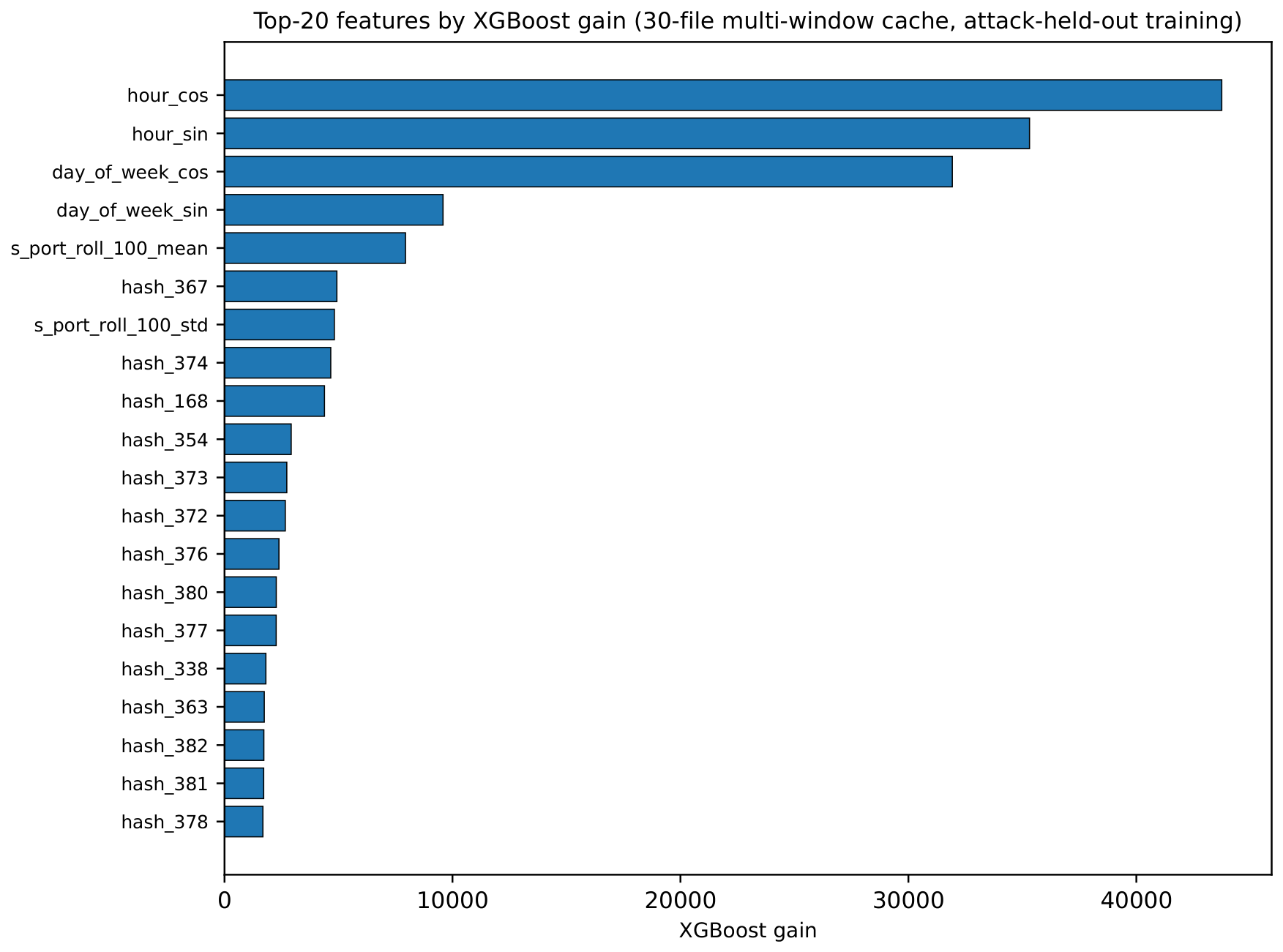
Figure 5 reports the top-20 features by gain for the XGBoost model trained on the 30-file multi-window cache under attack-held-out. The four highest-gain features are the cyclic time encodings (hour_sin, hour_cos, day_of_week_sin, day_of_week_cos). Because the SWaT attack catalogue places each attack at a particular wall-clock time, the classifier learns time-of-day as a strong proxy for “attack present”. When LOO holds out an attack whose execution time lies outside the training-time distribution, this proxy fails by construction: the model has learned to score the held-out attack’s time-of-day as normal even though the underlying attack-vector features are present. The dominance of time features in Figure 5 is therefore both empirical evidence for the signature-memorisation argument above and a direct critique of any SWaT IDS evaluation that does not control for attack-timing leakage.

7.2. Why the LSTM-Autoencoder Is Bimodal

The per-attack distribution of the LSTM-Autoencoder AUROC values in Table 6 contains nine attacks above $0.7$ (six above $0.8$) and seven attacks below $0.5$ (three below $0.1$). The split tracks the type of attack rather than its identity. Attacks that produce large physical excursions—a sensor reading driven outside its operating band, an actuator command issued out-of-sequence, or a Modbus function code outside the normal vocabulary—are detected reliably because their reconstruction error sits in the upper tail of the all-normal validation distribution. Attacks that interpolate inside the normal envelope—replay attacks, slow drift attacks, attacks that spoof a sensor toward a value within its normal range—are not detectable by reconstruction; the autoencoder reconstructs them as well as any normal sequence, by definition.

This is not a defect of the LSTM-Autoencoder architecture. It is a fundamental limit on what reconstruction-based anomaly detection can do irrespective of model capacity. Detecting in-envelope attacks requires either a positive label signal (which supervised methods exploit) or a model of the legitimate command sequence (e.g., a learnt grammar of allowed Modbus exchanges) that an autoencoder does not directly possess.

7.3. Threshold Tuning Is a First-Class Concern

The reported AUROC numbers are threshold-independent. In deployment, an IDS must commit to a threshold, which converts probabilities to alerts. The LSTM-Autoencoder achieves an AUROC of $0.85+$ on the most detectable attacks but, at the threshold equal to the 95^th percentile of normal-only validation reconstruction error, it only catches a fraction of those attack rows—the per-attack best-$F_1$ recall (a threshold-tuned operating point) is uniformly higher than the recall at the default threshold. Any honest reporting of IDS deployment readiness should therefore include both the threshold-independent ranking quality and an explicit operating-point analysis. We follow [25] in reporting both and recommend it as a standard.

7.4. Implications for Practitioners and Evaluators

Three concrete recommendations follow. For evaluators, report attack-held-out, or preferably leave-one-attack-out, alongside any random-split number on SWaT. The per-attack detectability map is more informative than any aggregate, particularly under bimodal distributions. For model designers, unsupervised reconstruction methods generalise better to unseen attack types than supervised classifiers, but the converse holds for in-envelope attacks; an ensemble that combines both is strictly more useful than either alone. For dataset curators, the fact that one quarter of the SWaT attacks are essentially undetectable by either family of models in our experiments suggests that the attack inventory itself is a meaningful axis of detector evaluation. Future ICS testbeds would benefit from attack catalogues that explicitly span the in-envelope versus out-of-envelope axis.

8. Conclusions, Limitations and Future Work

We revisited supervised and unsupervised machine-learning intrusion detection on the network-traffic modality of the SWaT dataset, extending a prior conference paper that reported strong AUROC under random stratified splits. Under stricter evaluation protocols—attack-held-out and leave-one-attack-out—the supervised XGBoost classifier drops from an AUROC of $0.884$ under random splits to a mean LOO AUROC of $0.315$ with per-attack AUROC below $0.5$ on the majority of held-out attacks. The unsupervised LSTM-Autoencoder retains the best solo mean LOO AUROC of $0.550$ across the 16 held-out attacks but exhibits a strongly bimodal per-attack distribution: it detects attacks that produce large physical excursions and misses attacks that interpolate inside the normal operating envelope. The two other supervised baselines score below random on the majority of folds (Bi-LSTM $0.215$; TCN $0.278$). The models’ detectable-attack sets are nearly disjoint, and a three-member sign-adjusted oracle-bound ensemble flips per-fold members whose AUROC inverts achieve a mean LOO AUROC of $0.844$ ($\sigma =0.104$) with per-attack AUROC values at or above $0.7$ on 14 of the 16 folds. Adding the TCN as a fourth ensemble member does not improve the result, which is evidence that the unseen-attack regime requires additional detection modes rather than additional supervised classifiers. We additionally report recall at a fixed $5\%$ FPR alongside threshold-independent AUROC, paired Wilcoxon significance tests, and bootstrap confidence intervals; the threshold-tuned $F_1$ and FPR-bounded recall are low across the board for every solo model.

This paper has clear limitations that we list explicitly so that the reader can correctly weight the conclusions.

• Sample size.

Our experiments operate on 15- and 30-file subsamples drawn diversely from the 737-file SWaT A6 corpus. The 30-file sample contains 17 of the 36 SWaT attack identifiers; the remaining attacks are not evaluated. The full dataset is approximately 100 GB and exceeds the in-memory budget of the streaming-free pipeline used here; a streaming loader (XGBoost ExtMemQuantileDMatrix and PyTorch IterableDataset over Parquet) is the principal item of future work and would unlock evaluation on all 737 files and all 36 attack identifiers.

• Single modality.

We work exclusively on SWaT network-traffic data. The physical-process modality, where rigorous unsupervised work is well established [25,26,27], is not evaluated here. A cross-modality study—training on network features, validating on process features, or training a fused model—would be a natural extension and would address the question of whether physical excursions detectable in process readings are predictable from contemporaneous network traffic.

• Single testbed.

SWaT is a single physical implementation of one water-treatment process. A model that performs well on SWaT need not generalise to a different plant; conversely, our protocol-gap finding would carry more weight if reproduced on the EPIC, MSU WADI or HAI testbeds. We have not yet performed this work; it would be the natural follow-up paper.

• Engineering boundary conditions.

The Bi-LSTM run encountered out-of-memory pressure during preliminary trials at batch_size $=1024$ on the 30-file leave-one-attack-out configuration; the results reported in Table 6 were obtained at batch_size $=256$ to fit the container’s 62 GB cgroup cap. The streaming data loader (above) would also remove this constraint and is part of the same future work.

• Preprocessing leakage in the feature scaler.

The StandardScaler is fit once on the union of all selected files before splitting (Section 3.2), so per-feature mean and standard deviation incorporate rows that subsequently become validation or test partitions. This is a known but limited form of leakage; we expect its practical impact to be small because the statistics are univariate and are dominated by the abundant normal-traffic rows that are present in every partition. A leakage-aware variant that re-fits the scaler on each fold’s training partition is straightforward but requires the streaming loader.

• Synthetic testbed traffic.

SWaT produces traffic from a controlled, scaled-down plant with a small fixed inventory of supervisory workstations and PLCs. Real-world utility networks include richer benign-traffic populations (engineering workstations, vendor remote access, monitoring agents, third-party telemetry), and statistical analyses of operational ICS captures consistently report distributional differences relative to testbed datasets. An unsupervised reconstruction-based detector tuned on SWaT normals would, in deployment, almost certainly experience higher false-positive rates from this richer benign distribution; conversely, a supervised classifier may fail to flag novel benign anomalies as “normal”. The narrowness of SWaT’s benign distribution should be considered when transferring numbers from this paper to operational settings.

• Detection of in-envelope attacks.

The LSTM-Autoencoder fails on attacks that interpolate inside the normal operating envelope (Section 6.2). Reconstruction-based detection is fundamentally limited here. Approaches that explicitly model inter-sensor or inter-flow relationships—the Graph Deviation Network [27] learns a directed graph over sensors and scores deviations with respect to predicted neighbour behaviour—are a promising complementary direction for SWaT and a natural follow-up.

• Deployable approximation of the sign-adjusted ensemble.

The headline ensemble result (mean LOO AUROC $0.844$) is an oracle bound: it consults the held-out labels to decide which members to flip per fold. A deployable approximation that estimates the per-attack sign from training-time signal alone (Section 6.3, options (i)–(iii)) is the principal modelling follow-up. Signature-clustering and few-shot calibration would be most readily integrated with the current pipeline; meta-learning the sign with a small auxiliary classifier requires additional held-out validation data not present in the 30-file cache.

• Online and continual learning.

All experiments here are offline: models train once on a fixed sample and are evaluated on disjoint attacks. Practical ICS IDSs must adapt to drift in benign traffic over weeks and months, and ideally, it ought to incorporate operator-confirmed labels as they accrue. Continual-learning approaches for IDSs (e.g., Cassales et al., reviewed in recent surveys) are a separate axis of follow-up and would interact non-trivially with the LOO evaluation framework introduced here.

• Inference latency and deployment costs.

We report training and inference timings in Section 5; we do not report end-to-end alert latency on a streaming source. A streaming evaluation harness against a captured SWaT A6 PCAP would complete the deployment-realism picture and is part of the same future engineering item as full-737-file LOO.

The principal methodological recommendation that follows is to report attack-held-out or leave-one-attack-out evaluation as standard for SWaT network-traffic IDS work alongside the per-attack detectability breakdown and at least one operating-point claim (e.g., recall at a specified false-positive-rate budget). The principal modelling recommendation is that no single supervised model family detects every attack class on this testbed under unseen-attack evaluation, and an honest IDS pipeline should combine reconstruction-based and signature-based detectors with explicit per-attack sign awareness. We release the full preprocessing, evaluation, and ensemble pipeline to support reproduction and extension.

References

1. Stouffer, K.; Falco, J.; Scarfone, K. Guide to Industrial Control Systems (ICS) Security; NIST Special Publication 800-82; National Institute of Standards and Technology (NIST): Gaithersburg, MD, USA, 2011.
2. Asghar, M.R.; Hu, Q.; Zeadally, S. Cybersecurity in Industrial Control Systems: Issues, Technologies, and Challenges. Comput. Netw. 2019, 165, 106946. [Google Scholar] [CrossRef] [Scilit]
3. Bhamare, D.; Zolanvari, M.; Erbad, A.; Jain, R.; Khan, K.; Meskin, N. Cybersecurity for Industrial Control Systems: A Survey. Comput. Secur. 2020, 89, 101677. [Google Scholar] [CrossRef] [Scilit]
4. Hu, Y.; Yang, A.; Li, H.; Sun, Y.; Sun, L. A Survey of Intrusion Detection on Industrial Control Systems. Int. J. Distrib. Sens. Netw. 2018, 14, 1550147718794615. [Google Scholar] [CrossRef] [Scilit]
5. Williams, T.J. The Purdue Enterprise Reference Architecture. IFAC Proc. Vol. 1993, 26, 559–564. [Google Scholar] [CrossRef] [Scilit]
6. Koay, A.M.Y.; Ko, R.K.L.; Hettema, H.; Radke, K. Machine Learning in Industrial Control System (ICS) Security: Current Landscape, Opportunities and Challenges. J. Intell. Inf. Syst. 2023, 60, 377–405. [Google Scholar]
7. European Union Agency for Cybersecurity (ENISA). ENISA Threat Landscape 2023; Technical Report; ENISA: Athens, Greece, 2023. [Google Scholar] [CrossRef] [PubMed]
8. Kavallieratos, G.; Amro, A.; Gkioulos, V.; Stamatescu, G.; Rantos, K.; Lagkas, T.; Demertzis, K.; Paterakis, F.; Lekidis, A.; Dalamagkas, C.; et al. Best-Practices-Based Training for Improving Cybersecurity in Power Grids. In Computer Security. ESORICS 2024 International Workshops; Springer Nature: Berlin/Heidelberg, Germany, 2025; pp. 344–359. [Google Scholar]
9. Slay, J.; Miller, M. Lessons Learned from the Maroochy Water Breach. In International Conference on Critical Infrastructure Protection; Springer: Boston, MA, USA, 2008; Volume 253, pp. 73–82. [Google Scholar] [CrossRef] [Scilit]
10. McLaughlin, S.; Konstantinou, C.; Wang, X.; Davi, L.; Sadeghi, A.R.; Maniatakos, M.; Karri, R. The Cybersecurity Landscape in Industrial Control Systems. Proc. IEEE 2016, 104, 1039–1057. [Google Scholar] [CrossRef] [Scilit]
11. Bundesamt für Sicherheit in der Informationstechnik (BSI). Die Lage der IT-Sicherheit in Deutschland 2014; Technical Report; BSI: Bonn, Germany, 2014. [Google Scholar]
12. Geiger, M.; Bauer, J.; Masuch, M.; Franke, J. An Analysis of Black Energy 3, CrashOverride, and TRISIS, Three Malware Approaches Targeting Operational Technology Systems. In Proceedings of the 2020 25th IEEE International Conference on Emerging Technologies and Factory Automation (ETFA); IEEE: New York, NY, USA, 2020; Volume 1, pp. 1537–1543. [Google Scholar]
13. Cherepanov, A. Win32/Industroyer: A New Threat for Industrial Control Systems; ESET White Paper; ESET: Bratislava, Slovak Republic, 2017. [Google Scholar]
14. Dragos, Inc. TRISIS: Analyzing Safety System Targeted Malware; Dragos Threat Report; Dragos, Inc.: Hanover, MD, USA, 2017. [Google Scholar]
15. CISA. DarkSide Ransomware: Best Practices for Preventing Business Disruption from Ransomware Attacks; CISA Alert AA21-131A; CISA: Arlington, VA, USA, 2021.
16. Cybersecurity and Infrastructure Security Agency (CISA). Compromise of U.S. Water Treatment Facility; CISA Advisory AA21-042A; CISA: Arlington, VA, USA, 2021.
17. Cybersecurity and Infrastructure Security Agency (CISA); Federal Bureau of Investigation (FBI); National Security Agency (NSA); Environmental Protection Agency (EPA); Israel National Cyber Directorate (INCD). IRGC-Affiliated Cyber Actors Exploit PLCs in Multiple Sectors, Including U.S. Water and Wastewater Systems Facilities; Joint Cybersecurity Advisory; CISA: Arlington, VA, USA, 2023.
18. U.S. Environmental Protection Agency. Water and Wastewater Sector—Incident Action Checklist: Cybersecurity; Technical Report; EPA: Washington, DC, USA, 2022.
19. CISA; FBI; EPA. Top Cyber Actions for Securing Water Systems; CISA Factsheet; CISA: Arlington, VA, USA, 2024.
20. Khraisat, A.; Gondal, I.; Vamplew, P.; Kamruzzaman, J. Survey of intrusion detection systems: Techniques, datasets and challenges. Cybersecurity 2019, 2, 20. [Google Scholar] [CrossRef] [Scilit]
21. Umer, M.A.; Junejo, K.N.; Jilani, M.T.; Mathur, A.P. Machine Learning for Intrusion Detection in Industrial Control Systems: Applications, Challenges, and Recommendations. Int. J. Crit. Infrastruct. Prot. 2022, 38, 100516. [Google Scholar] [CrossRef] [Scilit]
22. Goh, J.; Adepu, S.; Junejo, K.N.; Mathur, A. A Dataset to Support Research in the Design of Secure Water Treatment Systems. In Critical Information Infrastructures Security, CRITIS 2016; Lecture Notes in Computer Science; Springer: Cham, Switzerland, 2017; Volume 10242, pp. 88–99. [Google Scholar] [CrossRef] [Scilit]
23. Mathur, A.P.; Tippenhauer, N.O. SWaT: A Water Treatment Testbed for Research and Training on ICS Security. In Proceedings of the 2016 International Workshop on Cyber-Physical Systems for Smart Water Networks (CySWater); IEEE: New York, NY, USA, 2016; pp. 31–36. [Google Scholar]
24. Ahmed, C.M.; Palleti, V.R.; Mathur, A.P. WADI: A Water Distribution Testbed for Research in the Design of Secure Cyber Physical Systems. In Proceedings of the 3rd International Workshop on Cyber-Physical Systems for Smart Water Networks; Association for Computing Machinery: New York, NY, USA, 2017; pp. 25–28. [Google Scholar] [CrossRef] [Scilit]
25. Kravchik, M.; Shabtai, A. Detecting Cyber Attacks in Industrial Control Systems Using Convolutional Neural Networks. In Proceedings of the 2018 Workshop on Cyber-Physical Systems Security and PrivaCy (CPS-SPC); ACM: New York, NY, USA, 2018; pp. 72–83. [Google Scholar]
26. Li, D.; Chen, D.; Jin, B.; Shi, L.; Goh, J.; Ng, S.K. MAD-GAN: Multivariate Anomaly Detection for Time Series Data with Generative Adversarial Networks. In Proceedings of the Artificial Neural Networks and Machine Learning–ICANN 2019; Lecture Notes in Computer Science; Springer: Cham, Switzerland, 2019; Volume 11730, pp. 703–716. [Google Scholar] [CrossRef] [Scilit]
27. Deng, A.; Hooi, B. Graph Neural Network-Based Anomaly Detection in Multivariate Time Series. In Proceedings of the AAAI Conference on Artificial Intelligence; AAAI: Washington, DC, USA, 2021; Volume 35, pp. 4027–4035. [Google Scholar]
28. Mesca, S.; Stamatescu, G. Intelligent Intrusion Detection System for Cybersecurity of Water Utilities. In Proceedings of the 2025 24th RoEduNet Conference: Networking in Education and Research (RoEduNet); IEEE: New York, NY, USA, 2025. [Google Scholar]
29. Gangwar, A.; Sahu, S. A Survey on Anomaly and Signature Based Intrusion Detection System (IDS). Int. J. Eng. Res. Appl. 2014, 4, 67–72. [Google Scholar]
30. Kaouk, M.; Flaus, J.M.; Potet, M.L.; Groz, R. A Review of Intrusion Detection Systems for Industrial Control Systems. In Proceedings of the 2019 6th International Conference on Control, Decision and Information Technologies (CoDIT); IEEE: New York, NY, USA, 2019; pp. 1699–1704. [Google Scholar]
31. Stamatescu, G.; Stamatescu, I.; Arghira, N.; Făgărăşan, I. Cybersecurity Perspectives for Smart Building Automation Systems. In Proceedings of the 2020 12th International Conference on Electronics, Computers and Artificial Intelligence (ECAI); IEEE: New York, NY, USA, 2020; pp. 1–5. [Google Scholar]
32. Ibrahim, M.; Al-Wadi, A. Wastewater Treatment Plant Security Analysis. In Proceedings of the 2022 14th International Conference on Electronics, Computers and Artificial Intelligence (ECAI); IEEE: New York, NY, USA, 2022; pp. 1–6. [Google Scholar]
33. Ibrahim, M.; Elhafiz, R.; Al-Wadi, A. Reinforcement Learning-Based Attack Graph Analysis for Wastewater Treatment Plant. IEEE Trans. Ind. Appl. 2023, 59, 7858–7867. [Google Scholar] [CrossRef] [Scilit]
34. Verkerken, M.; D’hooge, L.; Wauters, T.; Volckaert, B.; De Turck, F. Towards Model Generalization for Intrusion Detection: Unsupervised Machine Learning Techniques. J. Netw. Syst. Manag. 2022, 30, 12. [Google Scholar] [CrossRef] [Scilit]
35. Hesford, J.; Cheng, D.; Wan, A.; Huynh, L.; Kim, S.; Kim, H.; Hong, J.B. Expectations Versus Reality: Evaluating Intrusion Detection Systems in Practice. arXiv 2024, arXiv:2403.17458. [Google Scholar] [CrossRef] [Scilit]
36. Malhotra, P.; Ramakrishnan, A.; Anand, G.; Vig, L.; Agarwal, P.; Shroff, G. LSTM-based Encoder-Decoder for Multi-sensor Anomaly Detection. In Proceedings of the ICML 2016 Anomaly Detection Workshop, New York, NY, USA, 24 June 2016. [Google Scholar]
37. Xi, C.; Wang, H.; Wang, X. A Novel Multi-Scale Network Intrusion Detection Model with Transformer. Sci. Rep. 2024, 14, 23239. [Google Scholar] [CrossRef] [Scilit] [PubMed]
38. Shang, W.; Qiu, J.; Shi, H.; Wang, S.; Ding, L.; Xiao, Y. An Efficient Anomaly Detection Method for Industrial Control Systems: Deep Convolutional Autoencoding Transformer Network. Int. J. Intell. Syst. 2024, 2024, 5459452. [Google Scholar] [CrossRef] [Scilit]
39. Lin, L.; Gu, A.; Min, F.; Zhou, S. Multi-Level Graph Attention Network-Based Anomaly Detection in Industrial Control System. Actuators 2025, 14, 210. [Google Scholar] [CrossRef] [Scilit]
40. Zhang, D.; Wang, M.; Bu, Y.; Yu, J.; Yang, L. PdGAT-ID: An Intrusion Detection Method for Industrial Control Systems Based on Periodic Extraction and Spatiotemporal Graph Attention. Comput. Secur. 2025, 149, 104210. [Google Scholar] [CrossRef] [Scilit]
41. Li, R.; Shen, H.; Zhang, Q.; Duan, H. An Edge-Enhanced GraphSAGE-Based Intrusion Detection Model for the Internet of Things. Clust. Comput. 2025, 28, 309. [Google Scholar] [CrossRef] [Scilit]
42. Zhang, X.; Zhao, R.; Jiang, Z.; Chen, H.; Ding, Y.; Ngai, E.C.H.; Yang, S.H. Continual Learning with Strategic Selection and Forgetting for Network Intrusion Detection. arXiv 2024, arXiv:2412.16264. [Google Scholar] [CrossRef] [Scilit]
43. Guo, C.; Li, X.; Cheng, J.; Yang, S.; Gong, H. Continual Learning for Intrusion Detection Under Evolving Network Threats. Future Internet 2025, 17, 456. [Google Scholar] [CrossRef] [Scilit]
44. Fang, J.; Xie, C. Unknown Intrusion Traffic Detection Method Based on Unsupervised Learning and Open-Set Recognition. Sci. Rep. 2025, 15, 17001. [Google Scholar] [CrossRef] [Scilit] [PubMed]
45. Yu, W.; Chen, Z.; Wang, H.; Miao, Z.; Zhong, D. Industrial Network Intrusion Detection in Open-Set Scenarios. Int. J. Inf. Secur. 2025, 24, 39. [Google Scholar] [CrossRef] [Scilit]
46. Qiu, Z.; Zhou, D.; Zhai, Y.; Liu, B.; He, L.; Cao, J. VAEMax: Open-Set Intrusion Detection Based on OpenMax and Variational Autoencoder. In Proceedings of the 5th International Conference on Information and Communication Technology (ICTC), Nanjing, China, 10–12 May 2024. [Google Scholar] [CrossRef] [Scilit]
47. Cantone, M.; Marrocco, C.; Bria, A. On Machine Learning in Network Intrusion Detection: A Cross-Dataset Generalization Study. IEEE Access 2024, 12, 144489–144508. [Google Scholar] [CrossRef] [Scilit]
48. Guo, X.F.; Meroño-Peñuela, A.; Maffeis, S.; Pierazzi, F. KnowML: Improving Generalization of ML-NIDS with Attack Knowledge Graphs. arXiv 2025, arXiv:2506.19802. [Google Scholar] [CrossRef] [Scilit]
49. Chen, T.; Guestrin, C. XGBoost: A Scalable Tree Boosting System. In Proceedings of the 22nd ACM SIGKDD International Conference on Knowledge Discovery and Data Mining; Association for Computing Machinery: New York, NY, USA, 2016; pp. 785–794. [Google Scholar] [CrossRef] [Scilit]
50. Hochreiter, S.; Schmidhuber, J. Long Short-Term Memory. Neural Comput. 1997, 9, 1735–1780. [Google Scholar] [CrossRef] [Scilit] [PubMed]
51. Schuster, M.; Paliwal, K.K. Bidirectional Recurrent Neural Networks. IEEE Trans. Signal Process. 1997, 45, 2673–2681. [Google Scholar] [CrossRef] [Scilit]
52. Wolpert, D.H. Stacked Generalization. Neural Netw. 1992, 5, 241–259. [Google Scholar] [CrossRef] [Scilit]
Figure 1. Purdue Enterprise Reference Architecture for industrial control networks. The Demilitarised Zone (Level 3.5) is the prescribed boundary between the OT (Levels 0–3) and IT (Levels 4–5) domains; in practice, this prescription is frequently violated. Adapted from [5,28].
Applsci 16 07206 g001
Figure 2. SWaT testbed architecture, reproduced from previous own work [28]; the original layout is based on the iTrust release [22,23].
Applsci 16 07206 g002
Figure 3. Preprocessing pipeline. The Google Cloud Storage-resident SWaT network logs are surveyed for attack-containing files, a diverse subset is selected, features are engineered and scaled in a streaming pass, and the resulting per-file Parquet cache is consumed by three evaluation protocols.
Applsci 16 07206 g003
Figure 4. Per-attack ROC curves under leave-one-attack-out evaluation on the 30-file multi-window cache. Each panel holds out one attack identifier; curves are coloured by model (XGBoost: red; LSTM-Autoencoder: blue; Bi-LSTM: green); the diagonal is random guessing. Inset AUROC values are computed on a 200 , 000 -row stratified subsample per fold for plotting tractability; the per-fold values in Table 6 use the full test partition. The bimodality of the LSTM-Autoencoder is visible: out-of-envelope attacks (e.g., 23, 25, 26, 28, 29) yield curves close to the upper-left corner while in-envelope attacks (19, 20, 27) yield curves close to the diagonal or below. Curves bulging below the diagonal correspond to the supervised-inversion regime quantified in Section 6.2.
Applsci 16 07206 g004
Figure 5. Top-20 features by XGBoost gain (model: 04_multiwindow_30files). The four highest-gain features are cyclical encodings of hour-of-day and day-of-week, which the classifier exploits as a proxy for attack presence during training and which fails by construction on attacks held out by LOO.
Applsci 16 07206 g005