Machine Learning-Based Compressive Strength Prediction and Multi-Objective Optimization of Ultra-High Performance Concrete

Abstract

The compressive strength of ultra-high-performance concrete (UHPC) is jointly influenced by multiple factors, including material composition, mixture proportion parameters, and curing regime. Conventional empirical methods are therefore insufficient to accurately characterize the highly nonlinear relationships involved. To improve the prediction accuracy of UHPC compressive strength and to achieve mixture proportion optimization that simultaneously considers mechanical performance, economic efficiency, and environmental impact, this study developed random forest (RF), artificial neural network (ANN), gradient boosting decision tree (GBDT), and extreme gradient boosting (XGBoost) models based on 810 publicly available UHPC experimental datasets. Model performance was evaluated using R², RMSE, MAE, and MAPE. To enhance the robustness of model validation, repeated K-fold cross-validation, sensitivity analysis with different random seed splits, and benchmark model comparisons were further introduced. The results indicate that the XGBoost model achieved superior predictive performance on both the test set and robustness validation, with test-set R², RMSE, MAE, and MAPE values of 0.9604, 7.77, 5.58, and 4.80, respectively. The model was further interpreted using SHAP, PDP, and ICE methods, and the results revealed that curing age, fiber content, silica fume content, and water-to-binder ratio were important variables affecting the compressive strength of UHPC. Furthermore, XGBoost was used as a surrogate model and coupled with NSGA-II and TOPSIS methods for multi-objective optimization. Under the constraints of compressive strength, water-to-binder ratio, superplasticizer-to-binder ratio, and absolute volume, a computationally recommended UHPC mixture proportion balancing strength, cost, and carbon emissions was obtained. This study provides a reproducible machine-learning-assisted approach for UHPC compressive strength prediction and low-carbon, cost-effective mixture proportion design.

1. Introduction

Ultra-High-Performance Concrete (UHPC) is a novel cementitious composite characterized by ultra-high strength, excellent durability, and high toughness. It is currently broadly used in fields such as long-span bridges, high-rise structures, marine engineering, and national defense engineering [1].

To further promote the application of UHPC, investigating its relevant mechanical properties is of particular importance. Compressive strength is one of the primary indices for evaluating the basic mechanical properties of concrete. Accurately predicting the compressive strength of UHPC is of great significance for optimizing mix proportion design and reducing costs. As a key index for evaluating the performance of UHPC, compressive strength is influenced by multiple factors, and traditional prediction methods exhibit limitations.

In recent years, owing to the rapid development of computer technology, artificial intelligence (AI) and big data analysis have experienced rapid advancement. As a branch of AI [2], Machine Learning (ML) has also been widely applied in predicting the compressive strength of concrete. Deng et al. [3] established three models—CNN, BP neural network, and SVM—to predict the compressive strength of recycled concrete by learning deep features, such as the water-to-cement ratio, recycled coarse aggregate replacement ratio, recycled fine aggregate replacement ratio, fly ash replacement ratio, and their interactions. Muhammad et al. [4] employed models such as Lasso, KNN, and SVR models to predict the compressive strength of self-compacting concrete. Zhou et al. [5] utilized an artificial neural network (ANN) to establish a compressive strength prediction model for UHPC and employed a genetic algorithm (GA) to reduce the cost of UHPC. Bolbolvand et al. [6] employed GB, LightGBM, XGBoost, CatBoost, ERT, and DNN models to predict the compressive strength of UHPC under different input parameters. Gu et al. [7] utilized the XGBoost and LightGBM algorithms to conduct a time-variant reliability analysis of the Bazimen landslide in the Three Gorges Reservoir Area, evaluated the importance of these parameters via SHAP analysis and partial dependence analysis, and finally balanced high performance, low carbon emissions, and economic feasibility by optimizing the steam curing process parameters.

Overall, previous studies have widely applied machine learning methods to the prediction of compressive strength in concrete and UHPC. However, several limitations remain. First, some studies mainly focus on the prediction accuracy of a single model, while systematic validation of model generalization ability and sensitivity to random data splitting is still limited. Second, UHPC mixture variables are strongly coupled. When feature importance, SHAP, or PDP results are directly used for physical interpretation, the effects of multicollinearity and mixture proportion constraints may be overlooked. Third, existing multi-objective optimization studies often consider only part of the strength, cost, and carbon emission objectives, while constraints related to W/B, superplasticizer dosage, absolute volume, and engineering feasibility are not fully incorporated. To address these issues, this study develops an integrated framework for UHPC compressive strength prediction, model interpretation, and multi-objective optimization. The framework compares the predictive performance of RF, ANN, GBDT, and XGBoost, and further introduces repeated K-fold cross-validation, random-seed-based split sensitivity analysis, benchmark model comparison, multicollinearity analysis, and interpretability methods including SHAP and PDP/ICE. These analyses are used to improve the robustness of model evaluation and the reliability of interpretation. On this basis, NSGA-II and TOPSIS are combined to optimize compressive strength, material cost, and carbon emissions, while constraints on W/B, SP/B, absolute volume, and minimum strength are introduced to obtain an engineering-feasible recommended UHPC mixture. The main contribution of this study lies in integrating robust validation, interpretability analysis, and constrained optimization into a unified workflow. This provides a reproducible computational approach for the low-carbon, cost-effective, and high-performance mixture design of UHPC.

2. Methods

2.1. Data Collection and Preprocessing

2.1.1. Data Collection

In this study, 810 experimental data points regarding the compressive strength of UHPC were collected from the Mendeley Data database [8]. The dataset is structured as an 810 × 14 matrix, where the first 11 variables represent the quantities of various raw materials per cubic meter of UHPC. These constituents include cement (C), slag (S), silica fume (SF), limestone powder (LP), quartz powder (QP), fly ash (FA), nano-silica (NS), aggregate (A), water (W), fibers (Fi), and superplasticizer (SP). The 12th feature is the curing temperature (T), the 13th feature is the curing age (Age), and the 14th feature is the corresponding compressive strength value (CS) of the UHPC samples. These data reflect the compressive strength performance of UHPC with different types and mix proportions under varying curing temperatures and ages.

Table 1. Descriptive statistics of the UHPC compressive strength data.

Input Parameter	Mean	Standard Deviation	Minimum	Maximum	Median	Skewness
C/(kg/m3)	737.91	173.46	270.00	1251.20	770.50	−0.23
S/(kg/m3)	25.19	74.37	0.00	375.00	0.00	3.01
SF/(kg/m3)	136.99	104.14	0.00	433.70	144.00	0.26
LP/(kg/m3)	41.93	133.13	0.00	1058.20	0.00	4.75
QP/(kg/m3)	33.27	79.67	0.00	397.00	0.00	2.28
FA/(kg/m3)	26.26	67.46	0.00	356.00	0.00	2.49
NS/(kg/m3)	3.64	7.78	0.00	47.50	0.00	2.53
A/(kg/m3)	1150.11	312.15	407.80	1992.00	1116.00	0.24
W/(kg/m3)	179.89	25.57	90.00	272.60	177.00	0.62
Fi/(kg/m3)	56.04	75.23	0.00	234.00	0.00	0.82
SP/(kg/m3)	30.03	13.99	1.10	57.00	30.20	−0.18
T/°C	23.92	16.21	20.00	210.00	21.00	9.13
Age/d	37.09	53.12	1.00	365.00	28.00	3.80
CS/MPa	123.13	40.24	28.51	220.50	122.30	0.0023

presents the descriptive statistics of the dataset.

To capture the synergistic effects among the components, this study constructed two interaction features [9]: the W/B ratio (W/B = W/(C + S + SF + FA + NS)), reflecting the proportional relationship between water and cementitious materials; and the superplasticizer ratio (SP/B = SP/(C + S + SF + FA + NS)), characterizing the dosage of superplasticizer relative to cement. Specifically, cement, slag, silica fume, fly ash, and nano-silica (NS) are classified as cementitious or supplementary cementitious materials (SCMs). Conversely, limestone powder and quartz powder function primarily as inert fillers and particle packing modifiers and are, therefore, excluded from the water-to-binder (W/B) ratio calculation. Following feature engineering, the input variables were expanded to 15 features.

2.1.2. Data Preprocessing

In this study, data processing primarily involved data cleaning and data normalization [10]. To ensure the reproducibility of the data analysis process, the raw dataset was first subjected to column name standardization, missing value inspection, duplicate sample checking, and outlier identification. Statistical screening revealed no missing values and 18 duplicate records in the initial dataset. These repeated records were carefully checked but were not removed. This is because the dataset was obtained from a public secondary database, and the available information was insufficient to determine whether these entries were erroneous duplicates or repeated experimental records reported in the original sources. For outlier detection, the Z-score method was utilized as an auxiliary tool; any sample with an absolute standardized value greater than 3 for a specific variable was flagged as a potential anomaly. It should be noted that, given the UHPC data was compiled from diverse literature sources and experimental conditions, inherent variations in material dosages and curing regimes are expected. Therefore, rather than simply discarding all statistical outliers, these instances were retained and recorded as natural data distribution variances, which are carefully addressed during subsequent model training and interpretation. Ultimately, a total of 810 data samples were finalized for model construction.

Table 2. Data preprocessing summary.

Item	Value
Original samples	810
Missing cells	0
Duplicated rows	18
Rows with |Z-score| > 3	106
Removed samples	0
Final samples used	810

is the data preprocessing summary.

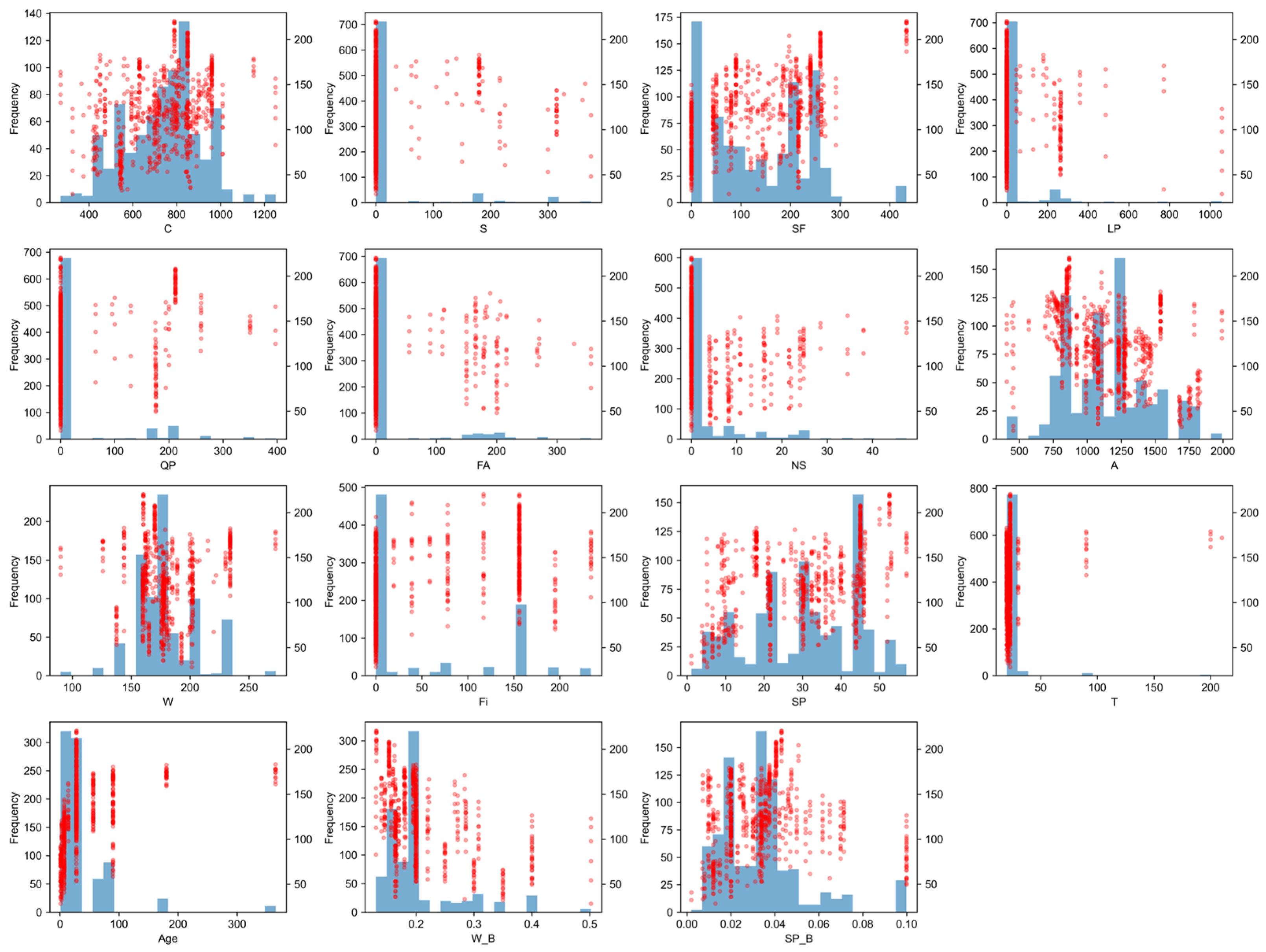
To prevent data leakage from the test set into the training process, data standardization was performed strictly after the dataset partitioning. Specifically, the dataset was first randomly split into a training set and a testing set at a 7:3 ratio, with a fixed random seed to ensure computational reproducibility. Subsequently, the standardization parameters (such as mean and standard deviation) were computed exclusively on the training set, and the identical scaling rules were then applied to the testing set. This procedure precludes the inadvertent introduction of test-set statistical information during the model training phase, thereby enabling a more objective evaluation of the models’ generalization capabilities. Although data standardization is not a prerequisite for tree-based algorithms, a uniform preprocessing pipeline was adopted across all algorithms. This ensures the training stability of models like Artificial Neural Networks (ANN) and Support Vector Regression (SVR), while maintaining a consistent input format for unbiased performance comparison. Figure 1 illustrates the distribution of the input variables and their relationships with compressive strength.

The histograms in Figure 1 illustrate the frequency distributions of each variable, while the red scatter points indicate the compressive strength levels of different samples with respect to that variable. The apparent differences in red intensity result from overlapping transparent markers and do not represent different variables or categories. Overall trends indicate that the water-to-binder (W/B) ratio exhibits a significant negative correlation with compressive strength. The contents of cement (C) and silica fume (SF) generally have a positive promoting effect on the strength, whereas fly ash (FA) and quartz powder (QP) may exert a negative impact on the strength when used in excess. Furthermore, the superplasticizer-to-binder (SP/B) ratio is predominantly concentrated within the range of 0.015 to 0.045, with the highest sample frequency observed around 0.035–0.045. In contrast, higher value intervals, such as 0.07 and 0.10, contain noticeably fewer samples, indicating a somewhat imbalanced distribution of this variable within the dataset. Furthermore, the scatter plot reveals no obvious monotonic relationship between the SP/B ratio and compressive strength, meaning that an increased superplasticizer dosage does not necessarily dictate an increase or decrease in strength. This suggests that the impact of the superplasticizer on the compressive strength of UHPC is not governed by a single factor; rather, it is the result of complex interactions with multiple variables, including the water-to-binder (W/B) ratio, the composition of cementitious materials, silica fume content, aggregate dosage, and curing age.

2.1.3. Correlation and Multicollinearity Analysis

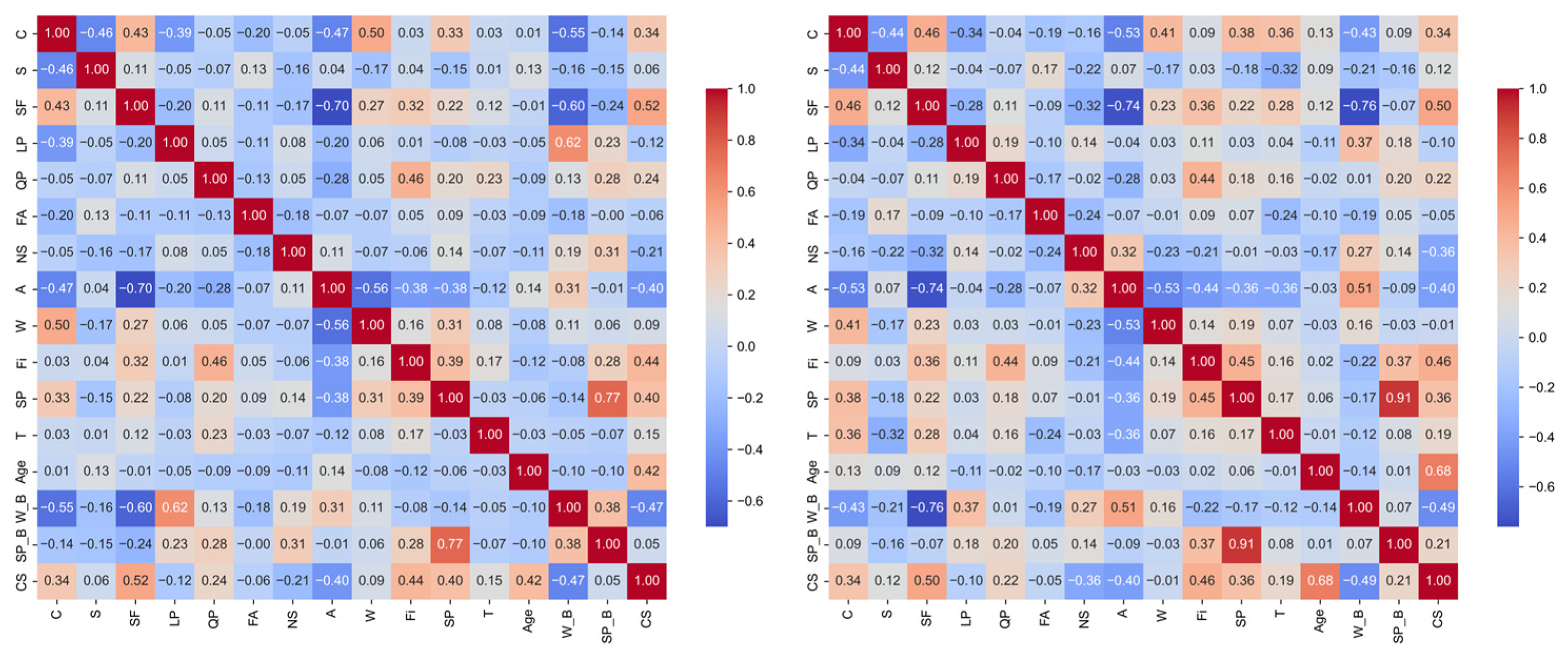
To analyze the correlations among the different input variables, as well as between the input variables and UHPC compressive strength, this study employs both Pearson and Spearman correlation coefficients for a comprehensive evaluation. The Pearson correlation coefficient is primarily used to measure the degree of linear correlation between continuous variables [11], whereas the Spearman correlation coefficient captures monotonic relationships, making it adaptable to non-linear monotonic trends. Combining these two metrics provides a more comprehensive understanding of the statistical associations among the UHPC mix proportions.

Figure 2 presents the Pearson and Spearman correlation coefficient matrices of the input variables.

As shown, varying degrees of correlation exist among the raw material dosages, curing parameters, and derived features. It is important to note that the UHPC mix design is inherently constrained by factors such as the water-to-binder ratio, total binder content, aggregate volume fraction, admixture dosage, and the absolute volume principle; consequently, these variables are not entirely independent. In particular, the W/B and SP/B features introduced in this study are computed directly from the primary material variables, defined as W/(C + S + SF + FA + NS) and SP/(C + S + SF + FA + NS), respectively. Therefore, while these derived variables hold explicit engineering significance, they inevitably exhibit certain correlations with the original components, such as water, cementitious materials, and the superplasticizer.

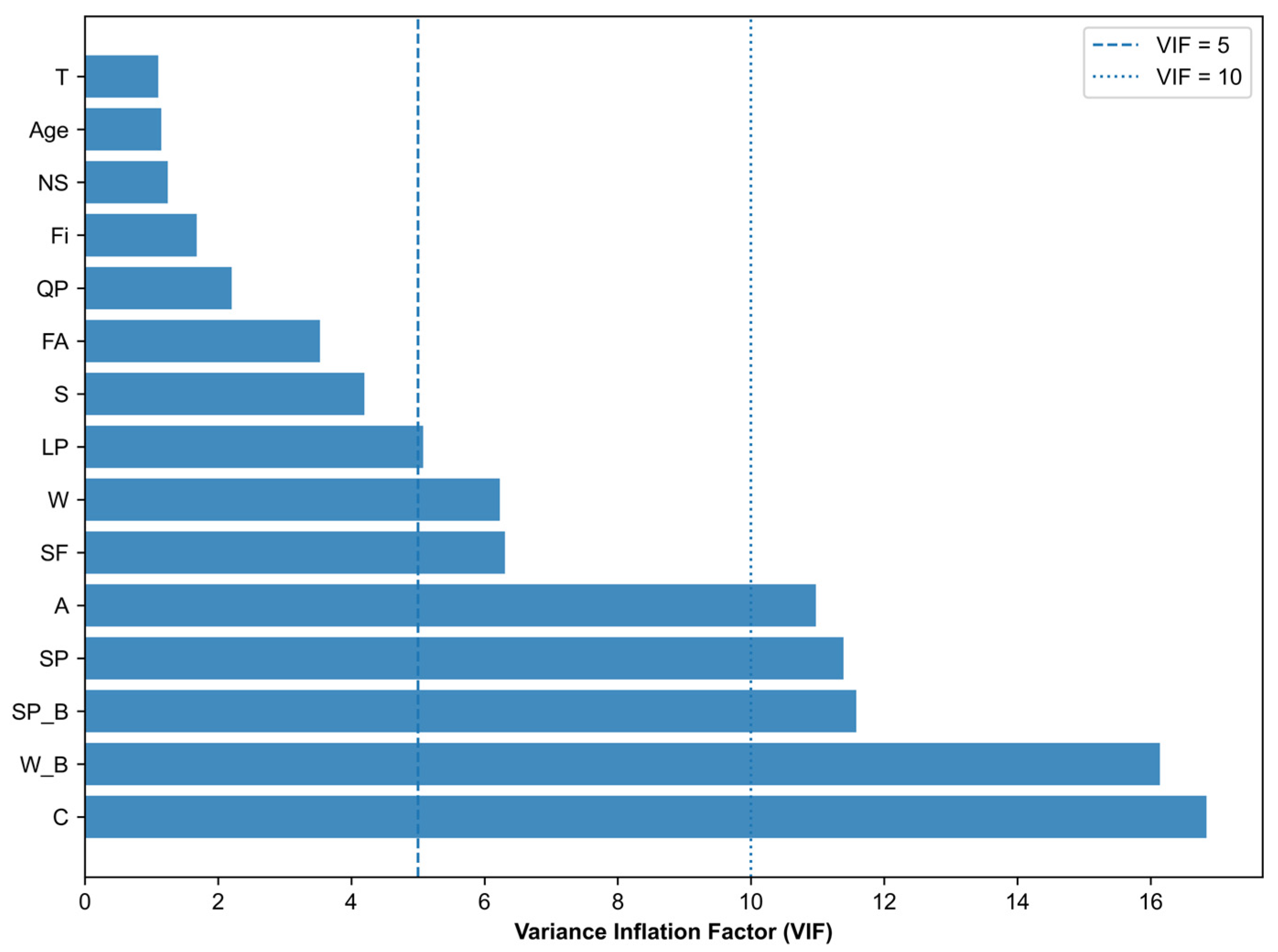
To further evaluate the impact of variable redundancy and multicollinearity on the model interpretation results, the Variance Inflation Factor (VIF) was employed to analyze the input variables, as illustrated in Figure 3.

As illustrated in Figure 3, the VIF values of the different input variables exhibit significant variations. Notably, the VIF values for C and W/B both exceed 10, indicating strong multicollinearity between these features and the other input variables. Similarly, the VIF values for SP, SP/B, and A also surpass 10, demonstrating strong correlations among the superplasticizer dosage, superplasticizer-to-binder ratio, aggregate content, and the remaining mix design variables. Furthermore, the VIF values for SF and W range between 5 and 10, suggesting a moderate degree of multicollinearity. In contrast, variables such as T, Age, NS, Fi, QP, FA, and S yield lower VIF values, which implies a relatively weak degree of linear redundancy between these features and the other inputs.

The occurrence of this phenomenon is justifiable, as the UHPC mix design is inherently governed by constraints such as the water-to-binder ratio, total binder content, aggregate volume fraction, superplasticizer dosage, and the absolute volume principle. In particular, W/B and SP/B are derived variables calculated directly from the water, cementitious materials, and superplasticizer; therefore, they inevitably exhibit certain correlations with the primary variables like C, W, SF, and SP. The rationale for retaining W/B and SP/B in this study lies in their explicit engineering significance, as they effectively reflect the combined impact of the water-binder proportion and relative admixture dosage on compressive strength. However, due to the presence of multicollinearity, the subsequent SHAP, PDP/ICE, and feature importance results should not be interpreted as the completely independent causal effects of a single variable. Instead, they should be understood as the statistical response patterns learned by the model under the given data distribution and mix formulation constraints.

2.2. Machine Learning Models and Analytical Methods

In order to systematically assess the predictive capabilities of different machine learning approaches on the compressive strength of UHPC, a comprehensive comparative analysis was conducted using four primary models: RF, ANN, GBDT, and XGBoost. Furthermore, Linear Regression (LR), Decision Tree Regression (DTR), and Support Vector Regression (SVR) were incorporated to serve as benchmark baselines.

2.2.1. Benchmark MODELS

To validate the effectiveness of advanced machine learning algorithms, Linear Regression (LR), Decision Tree Regression (DTR), and Support Vector Regression (SVR) were concurrently introduced as baseline models. Specifically, LR was employed to characterize the fundamental linear relationships between the input variables and compressive strength; DTR provided a predictive reference for a simple non-linear model; and SVR, representing traditional kernel-based machine learning methods, was used to benchmark non-linear regression capabilities. These baseline models were not intended to serve as the final surrogate models for multi-objective optimization. Instead, they were utilized for performance comparison against RF, ANN, GBDT, and XGBoost to determine whether more complex models could significantly enhance prediction accuracy and generalization capability. By comparing against these baselines, the pronounced non-linear and multi-factor coupled relationships between UHPC compressive strength and mix proportion parameters can be more clearly elucidated, thereby reinforcing the rationale behind the algorithmic selection.

2.2.2. Random Forest

Random Forest (RF) is an ensemble learning algorithm that enhances model performance by constructing multiple decision trees and aggregating their prediction results [12]. Its core principle lies in the introduction of dual randomness: first, utilizing bootstrap sampling to generate multiple training subsets (with each subset used to train an individual decision tree); and second, randomly selecting a subset of features—rather than the entire feature set—at each node split. This mechanism effectively reduces the bias and variance of individual trees, thereby enhancing the overall stability of the model. The advantages of Random Forest include its robust resistance to overfitting, its insensitivity to outliers, and its capacity to handle high-dimensional, non-linear data. These characteristics make it highly suitable for the multi-factor interaction scenarios present in UHPC strength prediction. However, its limitation lies in its dependence on hyperparameters (such as the number of trees), which necessitates optimization through cross-validation.

2.2.3. Artificial Neural Network

An Artificial Neural Network (ANN) is a computational model that simulates the connection structure and information processing mechanisms of neurons in the human brain. Its primary objective is to automatically learn underlying patterns through a data-driven approach, thereby solving non-linear and complex pattern recognition problems. The fundamental principle of an ANN lies in simulating the connectivity and signal processing logic of neurons in the human brain, utilizing artificial neurons as the basic building blocks to achieve collaborative learning [13]. First, a neuron receives input signals from the preceding layer (such as raw data or outputs from other neurons). Each input is multiplied by its corresponding weight, the magnitude of which reflects the relative influence of that input. Subsequently, all weighted inputs are summed, and a bias term is added. This bias serves to adjust the activation threshold of the neuron, thereby overcoming the limitation of an output dictated solely by the weighted sum of inputs. Finally, an activation function (e.g., Sigmoid or ReLU) is applied to the resultant sum to perform a non-linear transformation and generate the neuron’s final output signal; this non-linear transformation is the fundamental mechanism that enables an ANN to process complex problems. When a discrepancy exists between the predicted output and the actual value, the backpropagation algorithm is used to propagate the error from the output layer to the input layer. Based on the magnitude of this error, the weights and biases of each layer are iteratively adjusted. This iterative process continues until the error is reduced to an acceptable range, ultimately achieving the automatic learning of the underlying data patterns. Through the utilization of activation functions and multi-layer architectures, ANNs are capable of addressing non-linear problems that traditional linear models cannot resolve (such as image recognition and speech synthesis).

2.2.4. GBDT

The Gradient Boosting Decision Tree (GBDT) is an ensemble learning algorithm that constructs a robust strong learner by sequentially integrating multiple weak learners (typically shallow decision trees). Its fundamental principle involves first establishing an initial baseline model using the average output of the training samples. This is followed by an iterative training process: calculating the residual (or the negative gradient of the error) from the previous round’s ensemble model to serve as the target label for the current round, fitting a shallow decision tree to correct this error, determining a learning rate (step size) to govern the impact weight of the tree before updating the ensemble model, and finally computing the weighted sum of the predictions from all base trees. Its architecture utilizes shallow decision trees as base models and adopts a serial weighted ensemble strategy. Furthermore, it can be adapted for tasks such as classification and regression through the flexible selection of loss functions. While it possesses strong non-linear fitting capabilities, minimal requirements for data preprocessing, and relatively high interpretability (by outputting feature importance), it also presents several disadvantages. These include slow computational speeds due to the serial training of the base trees, sensitivity to outliers, complex parameter tuning, and poor adaptability to high-dimensional sparse data [14].

2.2.5. XGBoost

XGBoost (eXtreme Gradient Boosting) is an advanced ensemble learning algorithm based on the gradient boosting framework, the essence of which lies in constructing a strong learner through serial iteration [15]. The core concept of this algorithm is to utilize CART (Classification and Regression Tree) regression trees as weak learners. In each training iteration, a new tree is constructed along the negative gradient direction of the loss function based on the residuals of the preceding model. Model optimization is then achieved by minimizing an objective function composed of both a loss function and a regularization term. The advantages of this algorithm include: (1) approximating the objective function through a second-order Taylor expansion, thereby enhancing the optimization efficiency of gradient descent; (2) incorporating L1 (Lasso) and L2 (Ridge) regularization constraints to control feature weight sparsity and tree structure complexity, respectively, which effectively mitigates overfitting; (3) featuring a built-in automatic handling mechanism for missing values that learns the optimal splitting direction when sample features are missing, thus avoiding information bias caused by manual imputation; and (4) achieving parallel computation through feature pre-sorting and block storage, which significantly accelerates the training speed on large-scale datasets. The objective function [16] of XGBoost is expressed as

$$L(\theta )={\displaystyle {\displaystyle \sum _{i=1}^n}l(y_i,{\widehat{y_i}}^{(t)})}+{\displaystyle {\displaystyle \sum _{k=1}^t}\Omega (f_k)}$$

(1)

where $y_i$ is the actual value of the i-th sample; ${\widehat{y_i}}^{(t)}$ is the predicted value of the $i$-th sample at the $t$-th iteration; $l(y_i,\widehat{y_i})$ is the loss function measuring the difference between the actual and predicted values; and $\Omega (f_k)$ is the regularization term used to constrain the complexity of the tree and prevent model overfitting.

The formula for calculating $\Omega (f_k)$ is as follows:

$$\Omega (f_k)=\gamma T+{\displaystyle \frac{1}{2}}\lambda {\displaystyle \sum _{j=1}^T{{\omega }_j}^2}$$

(2)

where $\gamma$ and $\lambda$ are regularization parameters; $T$ represents the number of leaf nodes in the tree; and ${\omega }_j$ represents the sample weight on the $j$-th leaf node.

During the $t$-th iteration, building upon the prediction ${\widehat{y_i}}^{(t-1)}$ from the previous round, the model fits the first- and second-order gradient approximations of the loss function to derive a new weak learner $f_t(x)$. This process can be expressed as:

$${\widehat{y_i}}^{(t)}={\widehat{y_i}}^{(t-1)}+\eta f_t(x_i)$$

(3)

Through this iterative refinement, XGBoost is capable of gradually reducing the value of the loss function, continuously correcting the strength predictions, and ultimately enhancing the model’s predictive performance.

2.3. Evaluation Metrics for the Predictive Accuracy of Machine Learning Models

To quantitatively compare the differences among various models in predicting the compressive strength of UHPC, this study employs four metrics to evaluate the predictive models: the coefficient of determination (R²), Root Mean Square Error (RMSE), Mean Absolute Error (MAE), and Mean Absolute Percentage Error (MAPE). Their respective formulas [17] are as follows:

$$R^2=1-{\displaystyle \frac{{\displaystyle \sum _{i=1}^n{(y_i-\widehat{y_i})}^2}}{{\displaystyle \sum _{i=1}^n{(y_i-\stackrel{-}{y_i})}^2}}}$$

(4)

$$RMSE=\sqrt{{\displaystyle \frac{1}{n}}{{\displaystyle \sum _{i=1}^n(y_i-\widehat{y_i})}}^2}$$

(5)

$$MAE={\displaystyle \frac{1}{n}}{\displaystyle \sum _{i=1}^n\left|y_i-\widehat{y_i}\right|}$$

(6)

$$MAPE={\displaystyle \frac{1}{n}}{\displaystyle \sum _{i=1}^n\left|\frac{y_i-\widehat{y_i}}{y_i}\right|}\times 100\%$$

(7)

where $y_i$ is the actual value, $\widehat{y_i}$ is the predicted value, $\stackrel{-}{y_i}$ is the mean of the actual values, and $n$ is the total number of samples.

2.4. SHAP Analysis

To provide an in-depth explanation of the contribution of each input variable to the predictive outcomes of the machine learning models, this study employed the SHAP method, i.e., SHapley Additive exPlanations [18]. Based on Shapley values derived from cooperative game theory [19], the SHAP method decomposes model predictions into the sum of marginal contributions from individual features, thereby providing an interpretable description [20] of ‘black-box’ models. Its core concept is to measure the average marginal contribution of a specific feature by comparing the difference in the model’s predictive outcomes when the feature is included versus when it is excluded. This method is applicable not only to global explanations but also to local explanations, and its expression is as follows:

$${\varphi }_i(f,x)={\displaystyle \sum _{M\subseteq P\backslash \left\{i\right\}}\frac{\left|S\right|!(\left|P\right|-\left|M\right|-1)!}{\left|P\right|!}}·\left[f_x(M\cup \left\{i\right\})-f_x\left(M\right)\right]$$

(8)

where $P$ is the feature set; $M$ is any subset that does not include feature $i$; $\left|M\right|$ is the size of the set $S$; $\left|P\right|$ is the total number of features; and $f_x(M\cup \left\{i\right\})$ and $f_x(M)$ are the model’s prediction results including and excluding feature $i$, respectively.

In research concerning the prediction of UHPC compressive strength, SHAP analysis not only quantifies the importance of individual input variables but also reveals the positive and negative impacts of various features on the predictive outcomes [21], thereby providing a reliable interpretative basis for material design and construction optimization.

2.5. Partial Dependence Plot (PDP) Analysis

The Partial Dependence Plot (PDP) is an intuitive tool for interpreting machine learning models. Its core function is to isolate the confounding effects of other features and demonstrate, either individually or in pairs, the marginal relationship between a specific target feature and the model’s predictive outcomes. Its principle involves fixing the target feature $x_s$ and computing the marginal average over the remaining features to estimate the average impact of $x_s$ on the model’s predictions [22], which is expressed as:

$$PD(x_s)={\displaystyle \frac{1}{n}}{\displaystyle \sum _{i=1}^{n}f(x_s,x_c^{(i)})}$$

(9)

where $x_c$ represents the other features excluding $x_s$.

Through PDP, the trend of a target feature’s impact on predictive outcomes can be clearly determined (e.g., linear positive correlations, non-linear inflection points, or irrelevance). Furthermore, it enables the analysis of interaction effects between pairs of features (such as the joint influence of a two-feature combination on predictions). This makes it particularly suitable for the interpretability analysis of complex models (such as XGBoost and neural networks), aiding in the comprehension of the underlying logic of feature effects.

2.6. Multi-Objective Optimization

In practical engineering, it is often necessary to simultaneously consider multiple optimization objectives that are mutually conflicting or restrictive, such as structural safety versus cost-effectiveness, construction quality versus project duration, or seismic performance versus material consumption. These types of problems are difficult to effectively describe or solve using single-objective optimization methods; therefore, the introduction of Multi-objective Optimization (MOO) theory for systematic analysis is of significant importance. Multi-objective optimization refers to the problem of simultaneously optimizing two or more objective functions under a given set of constraints. Its general mathematical form can be expressed as:

$$\begin{array}{l}minF(x)=[f1(x),f2(x),\dots ,fm(x)]\\ s.t.\\ gi(x)\le 0,i=1,2,\dots ,p\\ hj(x)=0,j=1,2,\dots ,q\\ x\in \Omega \end{array}$$

(10)

where $x$ is the vector of design variables; $f_k(x)$ is the $k$-th objective function to be optimized; $g_i(x)$ and $h_j(x)$ represent the inequality and equality constraints, respectively; and $\Omega$ denotes the feasible region of the design variables.

Unlike single-objective optimization, multi-objective optimization problems typically do not possess a unique optimal solution. Instead, they form a set of Pareto optimal solutions A solution is defined as Pareto optimal if it is impossible to further improve at least one objective function without making any other objective function worse. The set composed of all Pareto optimal solutions in the objective space is known as the Pareto Front, which reflects the trade-off relationships between the various objectives. To solve multi-objective optimization problems, scholars have proposed various methods, which can be primarily classified into two categories:

• Traditional methods based on scalarization, such as the Weighted Sum method, the ε-constraint method, and the Ideal Point method. These methods solve the problem by transforming multiple objectives into a single objective; however, they are sensitive to weight coefficients or constraint parameters and often struggle to obtain a complete Pareto Front;
• Evolutionary algorithms based on swarm intelligence, such as Non-dominated Sorting Genetic Algorithms (NSGA-II, NSGA-III), Multi-objective Particle Swarm Optimization (MOPSO), and Multi-objective Differential Evolution algorithms. These methods do not require explicit scalarization of the objective functions and are capable of obtaining a uniformly distributed Pareto solution set in a single simulation run. Consequently, these methods have been widely applied to complex engineering optimization problems in recent years.

In the practical design of UHPC mix proportions, it is necessary to pursue ultimate mechanical performance while remaining constrained by economic budget limitations; simultaneously, one must respond to global ‘dual carbon’ goals by reducing the carbon emissions of the concrete. However, these objectives are often mutually conflicting. For instance, to enhance strength, it is typically necessary to increase the dosages of cement and silica fume; however, this inevitably leads to a surge in costs and a significant rise in carbon emissions. To resolve this complex non-linear trade-off problem, this study introduces the Non-dominated Sorting Genetic Algorithm II (NSGA-II). This algorithm can simultaneously handle multiple conflicting objective functions and identify a Pareto-optimal set rather than a single optimal solution, thereby providing decision-makers with a diverse range of alternatives. Based on the predicted compressive strength of UHPC, this study further employed the NSGA-II algorithm to optimize the carbon emissions and material cost objectives of UHPC. The ultimate goal is to achieve a multi-objective balance characterized by optimal mechanical performance, minimized environmental impact, and lowest economic cost.

3. Results and Discussion

3.1. Hyperparameter Optimization of Machine Learning Models

In this study, the collected data for all selected machine learning models were divided into a training set and a testing set at a ratio of 7:3. The training set was employed to construct performance-optimized machine learning models, while the testing set was utilized to verify and evaluate the generalization capability of the constructed models. Hyperparameter optimization is of critical importance in the development of these machine learning models. To ensure each model operates at its optimal state, this study employs Grid Search [23] (GridSearchCV) combined with 5-fold cross-validation to perform hyperparameter optimization for all models. To rigorously assess model robustness beyond the conventional 70/30 train-test split, this study additionally incorporates repeated K-fold cross-validation and random seed sensitivity analysis. The former examines the average predictive stability and variance across distinct data subsets, while the latter verifies that model performance is not merely an artifact of a specific data partition. This multifaceted validation approach ensures a comprehensive evaluation of generalization capabilities, thereby mitigating the risk of drawing biased conclusions from a singular train-test split.

Table 3. Hyperparameter search space and optimal parameters.

Model	Model Type	Hyperparameter Search Space	Optimal Hyperparameters
Linear Regression	Baseline Linear Model	No hyperparameter tuning	—
Decision Tree	Baseline Non-linear Model	max_depth = 8	max_depth = 8
SVR	Baseline Kernel-based Model	Kernel = ‘rbf’; C = 100; gamma = ‘scale’; epsilon = 0.1	fixed hyperparameters
RF	Tree-based Ensemble Model	n_estimators = [200, 300]; max_depth = [8, 10]; min_samples_split = [2, 4]	{‘max_depth’: 10, ‘min_samples_split’: 2, ‘n_estimators’: 200}
GBDT	Gradient Boosting Ensemble Model	n_estimators = [500, 1000]; max_depth = [3, 5]; learning_rate = [0.01, 0.05]; subsample = [0.8, 0.9]	{‘learning_rate’: 0.05, ‘max_depth’: 5, ‘n_estimators’: 1000, ‘subsample’: 0.9}
ANN	Artificial Neural Network Model	hidden_layer_sizes = [(8,),(16,),(32,),(12,8),(16,10),(32,16)]; learning_rate_init = [ 0.001,0.01]; alpha = [0.0001, 0.001]; max_iter = 1500	{‘alpha’: 0.001, ‘hidden_layer_sizes’: (32,), ‘learning_rate_init’: 0.01, ‘max_iter’: 1500}
XGBoost	Gradient Boosted Tree Model	n_estimators = [1000]; learning_rate = [0.01, 0.03]; max_depth = [3, 5]	{‘learning_rate’: 0.03, ‘max_depth’: 5, ‘n_estimators’: 1000}

summarizes the optimal hyperparameter configurations for each model.

As shown in Table 3, the Linear Regression (LR) model, serving as the baseline linear model, does not involve hyperparameter tuning. The Decision Tree model, acting as the baseline non-linear model, has its maximum depth fixed at 8. The SVR model employs a Radial Basis Function (RBF) kernel with fixed hyperparameters, specifically C = 100, γ = ‘scale’, and ϵ = 0.1. Regarding the ensemble models, the Random Forest (RF) model achieves optimal performance with 200 decision trees, a maximum depth of 10, and a minimum samples split of 2. The GBDT model performs best with 1000 weak learners, a maximum depth of 5, a learning rate of 0.05, and a subsample ratio of 0.9. For the Artificial Neural Network (ANN) model, the optimal architecture consists of a single hidden layer with 32 neurons, utilizing a learning rate of 0.01, an L₂ regularization parameter α = 0.001, and a maximum of 1500 iterations. Furthermore, the XGBoost model attains optimal performance with 1000 weak learners, a maximum depth of 5, and a learning rate of 0.03.

3.2. Machine Learning Model Performance

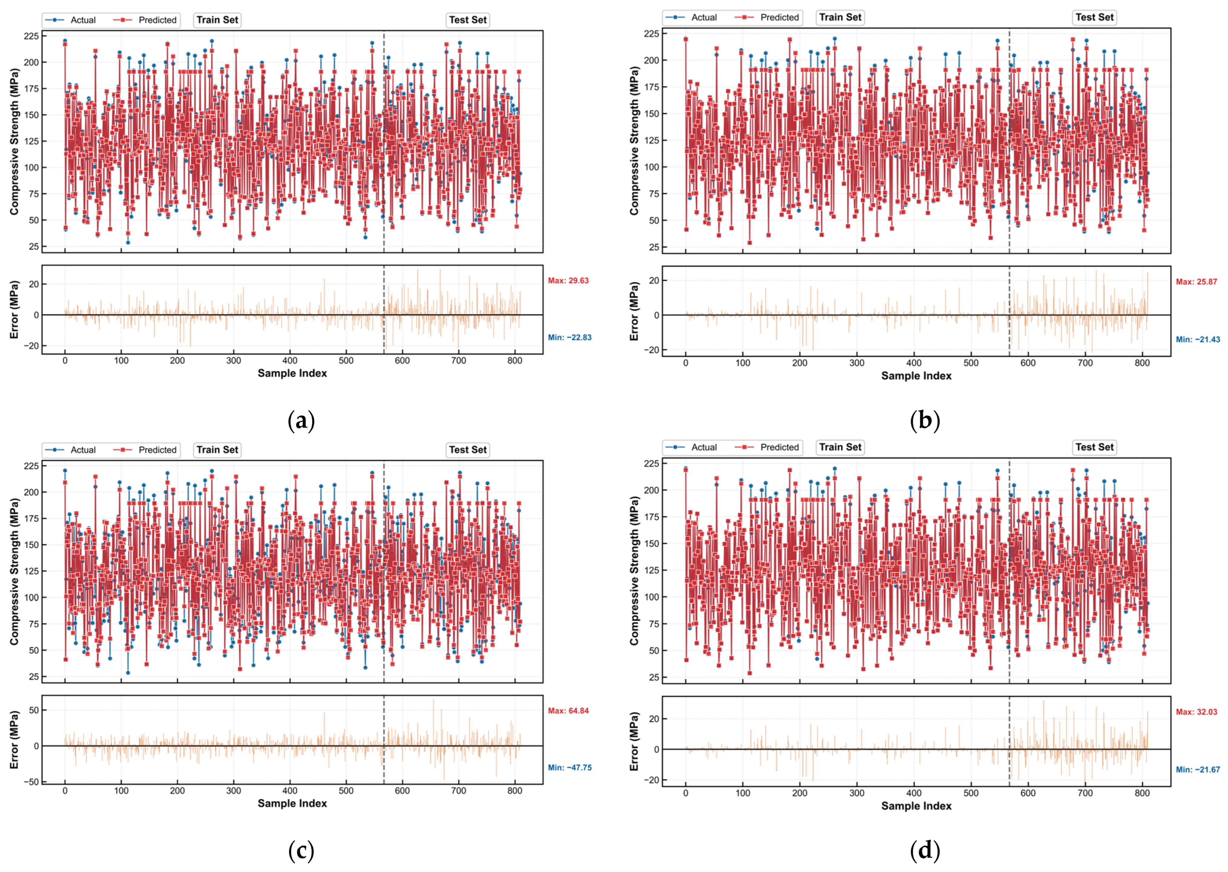
The machine learning models were trained using the hyperparameters detailed in Table 3. Subsequently, these models were utilized to generate the predicted UHPC compressive strength values for both the training and testing sets, as illustrated in Figure 4.

The blue data points represent the actual compressive strength values of the UHPC, the red data points denote the predicted compressive strength values generated by the machine learning models, and the yellow lines indicate the error between the predicted and actual values.

As observed from the training-set results in the figure, all four models, namely RF, XGBoost, ANN, and GBDT, demonstrate good capability in predicting the compressive strength of UHPC. The XGBoost and GBDT models exhibit similar and relatively low maximum absolute and average errors, followed by the RF model. Conversely, the ANN model yields the highest maximum absolute and average errors, resulting in the poorest predictive performance. For the testing set, the XGBoost and GBDT models similarly maintain the best predictive performance. The predictive performance of the RF model ranked next. Comparatively, the ANN model demonstrated the poorest predictive performance. These data demonstrate that the compressive strength values predicted by the four machine learning models closely align with the actual values, indicating that the four proposed models possess a certain capability for predicting the compressive strength of UHPC.

In this study, four evaluation metrics—R², RMSE, MAE, and MAPE—are employed to comprehensively evaluate and compare the four machine learning models. R² represents the model’s capacity to explain the variance within the data, with its value ranging from 0 to 1. A value closer to 1 indicates a better goodness-of-fit for the model. RMSE is utilized to measure the degree of discrepancy between the predicted and actual values; a lower value indicates a higher predictive accuracy of the model. MAE represents the average of the absolute errors between the predicted and observed values, serving to reflect the absolute magnitude of the prediction error; a lower value indicates a more accurate model prediction. MAPE is a statistical metric employed to evaluate the accuracy of predictive models. It measures the average percentage difference between the predicted and actual observed values; a lower value indicates a higher degree of model accuracy.

Table 4. Performance evaluation results of the machine learning model.

Model	Dataset	R2	RMSE	MAE	MAPE
Linear	Training Set	0.7202	21.53	17.24	17.23
	Test Set	0.7066	21.14	16.34	14.59
DecisionTree	Training Set	0.9781	6.03	3.82	3.03
	Test Set	0.9118	11.59	8.57	7.52
SVR	Training Set	0.8978	13.01	8.26	9.32
	Test Set	0.8542	14.90	10.57	10.18
RF	Training Set	0.9869	4.66	3.22	2.77
	Test Set	0.9529	8.47	6.29	5.40
XGBoost	Training Set	0.9933	3.33	1.72	1.38
	Test Set	0.9604	7.77	5.58	4.80
ANN	Training Set	0.9180	11.66	9.17	9.18
	Test Set	0.8698	14.08	10.50	9.29
GBDT	Training Set	0.9935	3.29	1.62	1.29
	Test Set	0.9540	8.37	5.88	5.05

presents the results of the performance evaluation metrics for each machine learning model.

As indicated by the data presented in the table, within the training set, although the R² of the GBDT model marginally exceeds that of the XGBoost model by 0.0002, it is 0.0064 lower than that of the XGBoost model on the testing set. Furthermore, the RMSE, MAE, and MAPE metrics all demonstrate that the XGBoost model exhibits the best predictive performance, achieving R² values of 0.9933 and 0.9604 on the training and testing sets, respectively. Closely following is the GBDT model, which achieved R² values of 0.9935 and 0.9540 on the training and testing sets, respectively. The RF model ranks next, yielding R² values of 0.9869 and 0.9529 on the training and testing sets, respectively. A comparison between the training and testing set results reveals that the R² of the ANN model on the training set is significantly higher than that on the testing set, indicating a certain risk of overfitting on the current UHPC dataset. This phenomenon can likely be attributed to the ANN’s high sensitivity to sample size, network architecture, initial weights, and hyperparameter settings. To mitigate the impact of overfitting, this study further conducted a sensitivity analysis on the ANN’s hidden layer structure, while introducing early stopping and the L2 regularization parameter α to constrain model complexity. Even after applying regularization, the R² of the ANN model on the training set remains significantly higher than that on the testing set. This indicates that its generalization capability on the current dataset of 810 UHPC samples is not as stable as that of XGBoost.

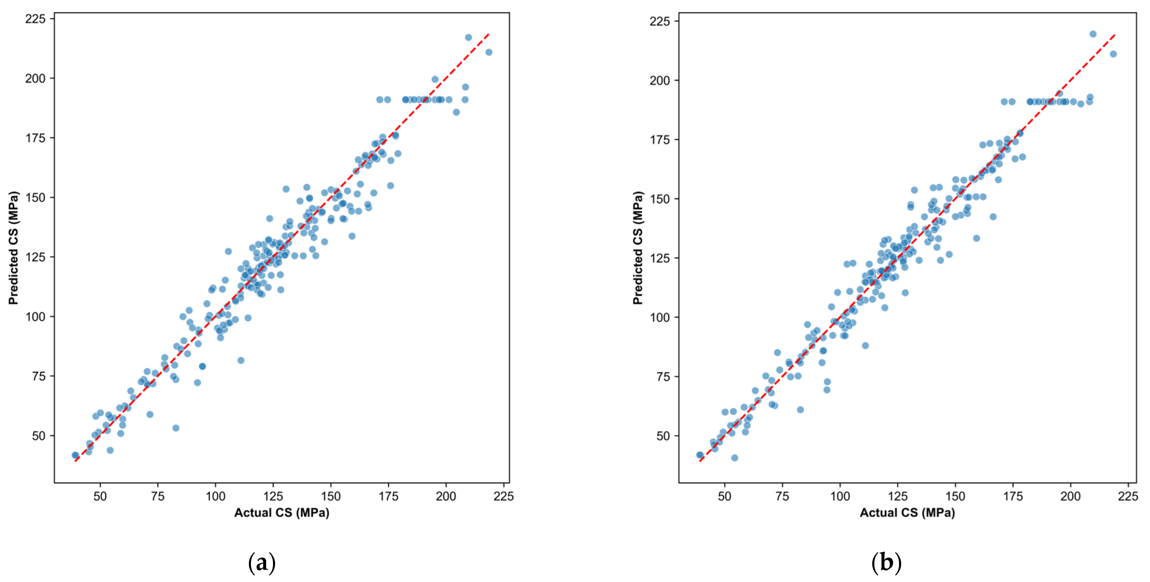
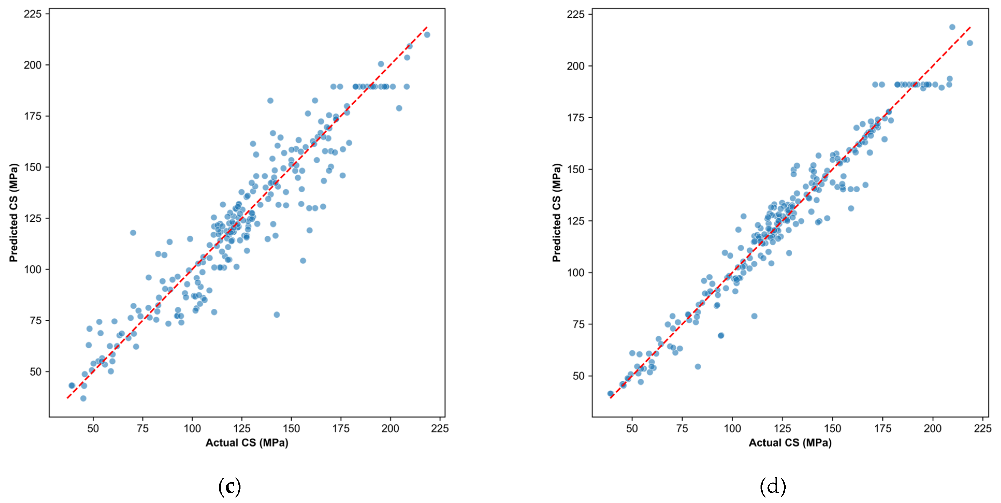
Figure 5 presents the scatter plots of the prediction results on the test set for selected machine learning models. The blue markers show the predicted compressive strengths against the corresponding experimental values, whereas the red dashed line denotes perfect agreement. Most data points lie close to this line, indicating good consistency between the model predictions and the measured results.

As can also be observed from the figure, the predicted values of the XGBoost model are more tightly clustered around the ideal line, indicating its superior predictive performance.

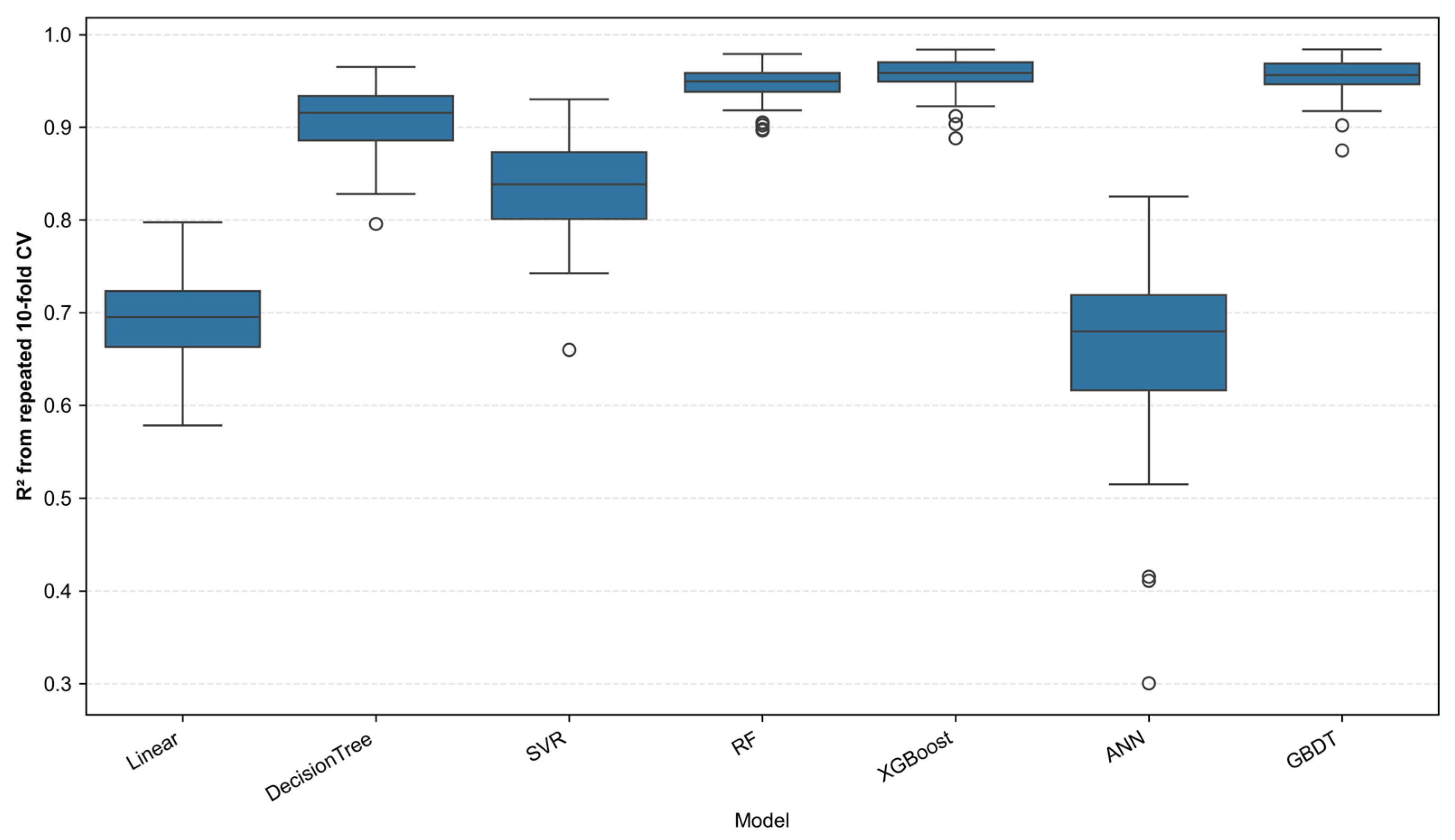
To avoid the randomness inherent in relying solely on a single 7:3 train-test split, this study conducted further model robustness validation alongside the conventional testing set evaluation. A two-stage cross-validation strategy was employed. The first stage focused on hyperparameter optimization, utilizing 5-fold cross-validation combined with GridSearchCV to search for the key parameters of each model, thereby balancing computational efficiency and parameter selection stability. The second stage evaluated the model’s generalization capability; after determining the optimal hyperparameters for each model, repeated 10-fold cross-validation was applied to test the robustness of the model’s performance. Specifically, this repeated 10-fold cross-validation partitioned the dataset into 10 subsets and was iterated 5 times, yielding a total of 50 sets of validation results. This approach allows for a more comprehensive reflection of the average predictive capability and performance fluctuation across different data partition conditions. The results of the repeated 10-fold cross-validation are presented in Figure 6.

As can be observed from the figure, the predictive performance of the different models varies across the repeated cross-validations. Notably, the R² distribution of the XGBoost model is generally higher, and its boxplot range is relatively narrow, indicating that its predictive results across different data subsets are highly stable with superior generalization capability. RF and GBDT also exhibit strong non-linear fitting capabilities, although the fluctuations in their validation results are more pronounced. In contrast, the ANN model is heavily influenced by network architecture, initial weights, and sample partitioning, leading to relatively higher volatility in its cross-validation results. The baseline models—such as Linear Regression, Decision Tree, and SVR—yield an overall performance inferior to that of the ensemble learning models. This demonstrates that complex non-linear models are better suited for characterizing the relationship between UHPC mix parameters and compressive strength.

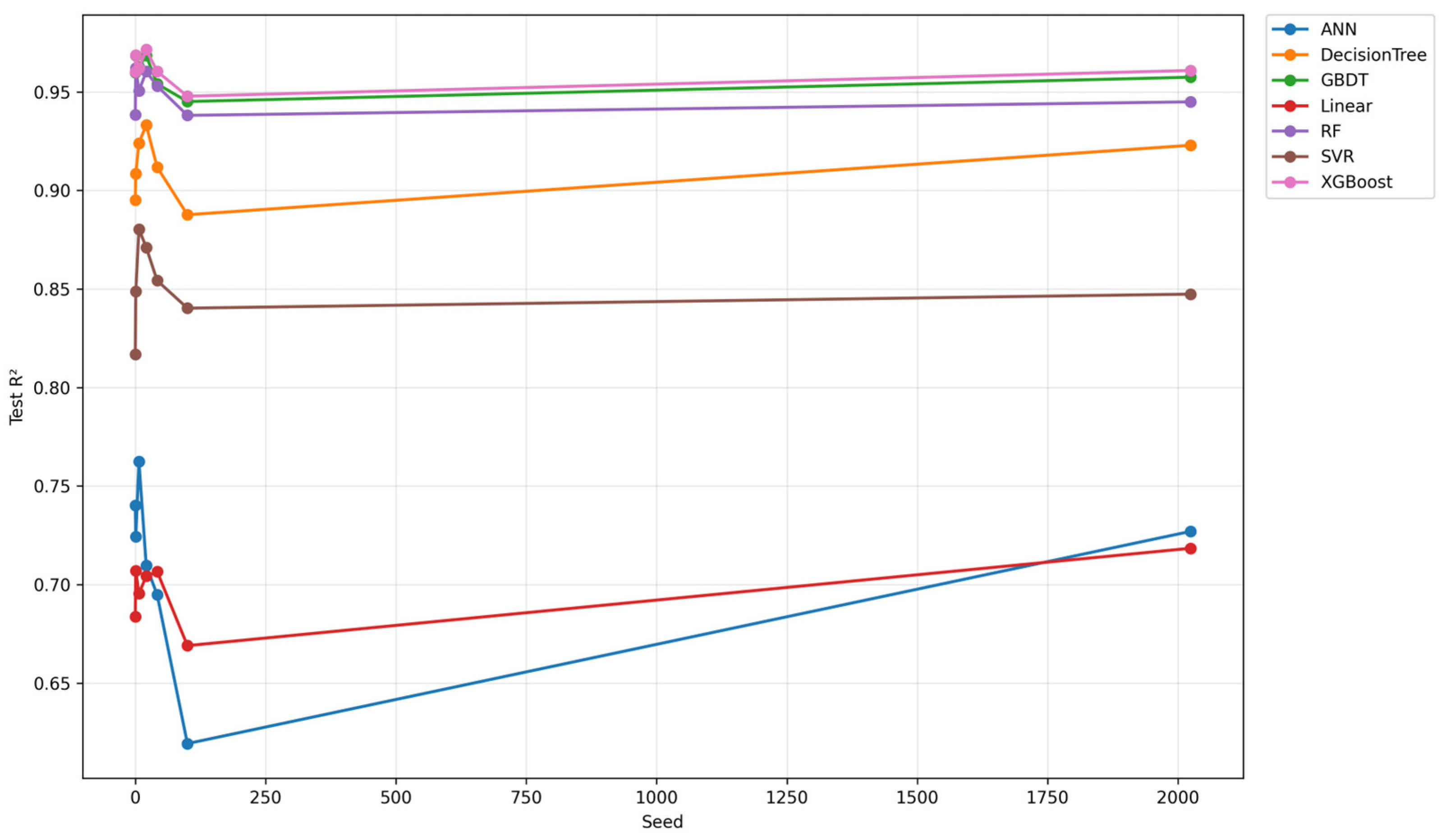
In addition to repeated cross-validation, this study further conducts a sensitivity analysis using 7:3 data splits under different random seeds to assess whether model performance is dependent on a specific train-test set partition. Specifically, multiple random seeds were established to re-partition the dataset, and the models were respectively trained and tested under an identical modeling workflow. The R², RMSE, and MAE of each model were then compared across these different splitting conditions. The results of the random split sensitivity analysis are presented in Figure 7.

The results indicate that the XGBoost model maintains a high and relatively stable testing set R² across different random seed conditions, demonstrating that its superior predictive performance is not an artifact of a coincidental data split. In contrast, the ANN and several baseline models are more sensitive to data partitioning, exhibiting more pronounced fluctuations in their testing set performance.

The aforementioned results demonstrate that XGBoost exhibits superior performance in terms of both predictive accuracy and robustness. Consequently, this study selects XGBoost as the surrogate model for the subsequent SHAP interpretability analysis and NSGA-II/TOPSIS multi-objective optimization.

3.3. Feature Importance Analysis

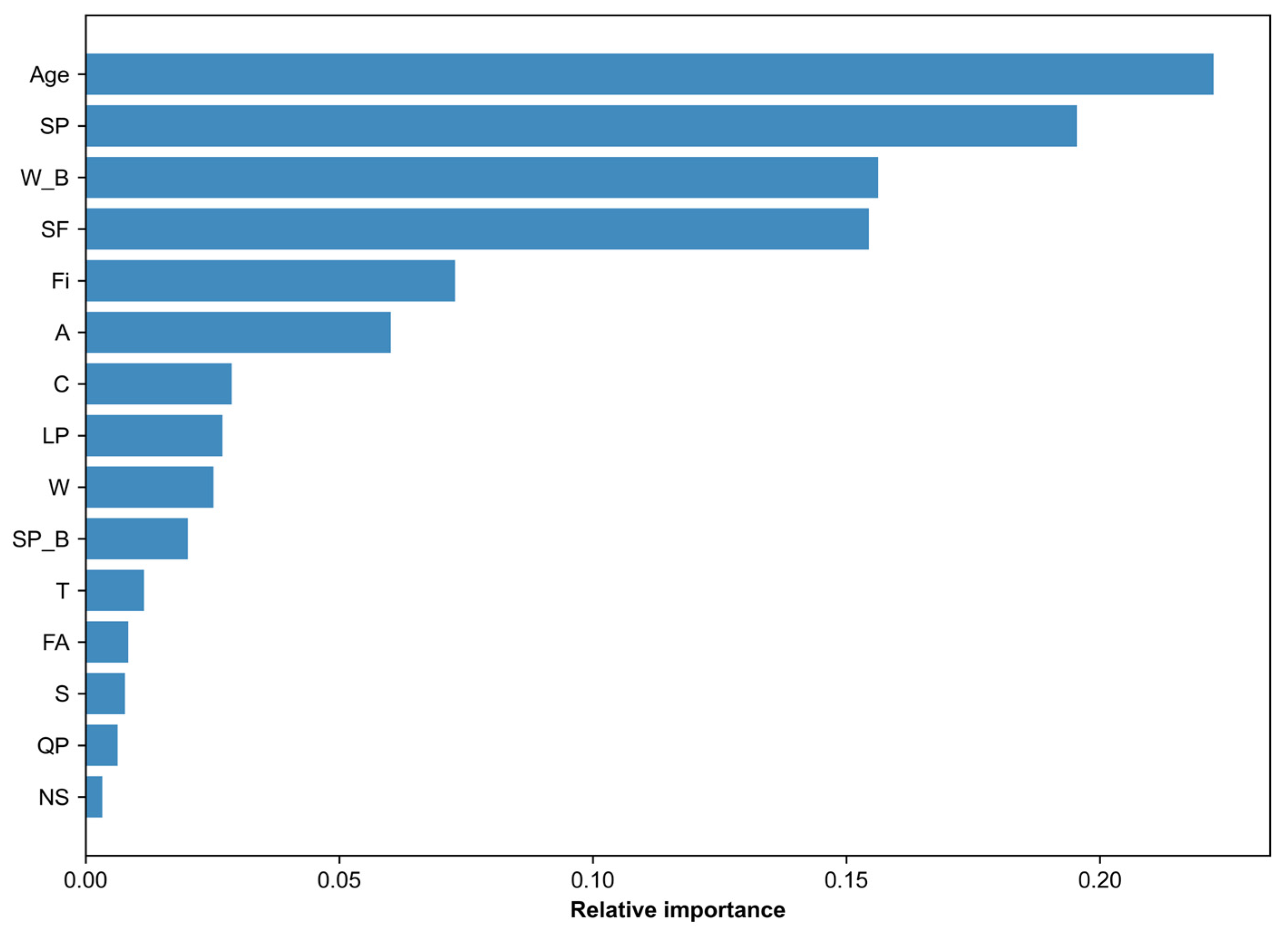
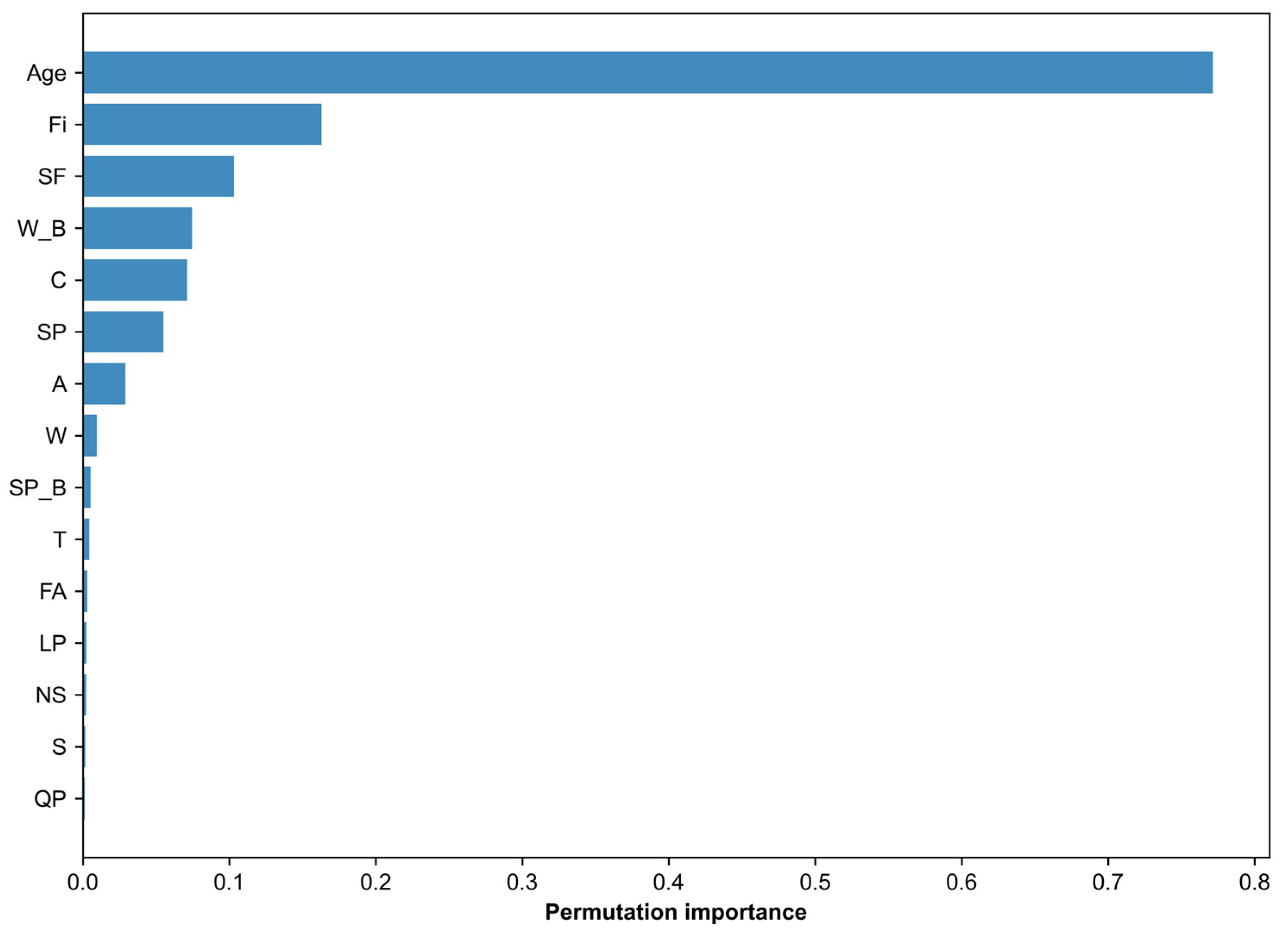
The impact of various factors on the compressive strength of UHPC may exhibit significant variations; therefore, elucidating the relative importance of the input parameters holds crucial guiding significance for the design of UHPC. Given that XGBoost has been previously identified as the optimal predictive model, this study analyzes feature importance utilizing XGBoost’s built-in feature importance and permutation importance. XGBoost’s built-in feature importance serves as a metric to evaluate the contribution of each feature to the model’s predictions, and it is calculated primarily based on the splitting process within the tree models [24]. It quantifies the degree of feature importance by calculating metrics such as the number of times a feature is utilized as a splitting node across all trees (Frequency), the reduction in loss achieved by each split (Gain), or the number of samples involved in the split (Cover). Permutation importance is an approach utilized to evaluate a feature’s contribution to the model by randomly shuffling its feature values. Specifically, it operates by randomly shuffling the values of a given feature (thereby disrupting the original correlation between that feature and the target variable) while keeping all other features constant. Subsequently, the model makes new predictions, and the resulting change in predictive performance is calculated. If a specific feature is highly important, randomly shuffling its values will lead to a substantial decline in model performance; conversely, if a feature is relatively unimportant, the resulting change in performance will be minimal. This method is independent of the model type and is applicable to all kinds of machine learning models. It can more intuitively reflect the actual influence of features on the prediction results, and is therefore commonly utilized to verify or supplement the model’s built-in feature importance assessments. Figure 8 and Figure 9 present the XGBoost built-in feature importance and permutation importance, respectively.

It can be observed from both figures that Age ranks first in both evaluation methods, indicating that Age is the most critical feature in the model’s predictions and exerts a significant influence on the results. This is primarily attributed to the hydration products generated by the prolonged hydration reaction of materials such as cement, silica fume, and fly ash in UHPC, which fill pores and interweave to form a dense hardened matrix, thereby enhancing the compressive strength. SF and W/B also demonstrate a high degree of impact in both evaluation methods. Specifically, due to its extremely fine particle size, SF effectively fills the interstices between cement particles, while its abundant reactive silica engages in a secondary pozzolanic reaction with the hydration product Ca(OH)₂ to produce additional C-S-H gel, ultimately elevating the strength of the matrix.

Furthermore, if the W/B ratio is too low, the binder materials cannot fully hydrate; conversely, if the ratio is too high, the evaporation of excess water creates a large number of internal voids, thereby decreasing the compactness.

3.4. SHAP Analysis Results

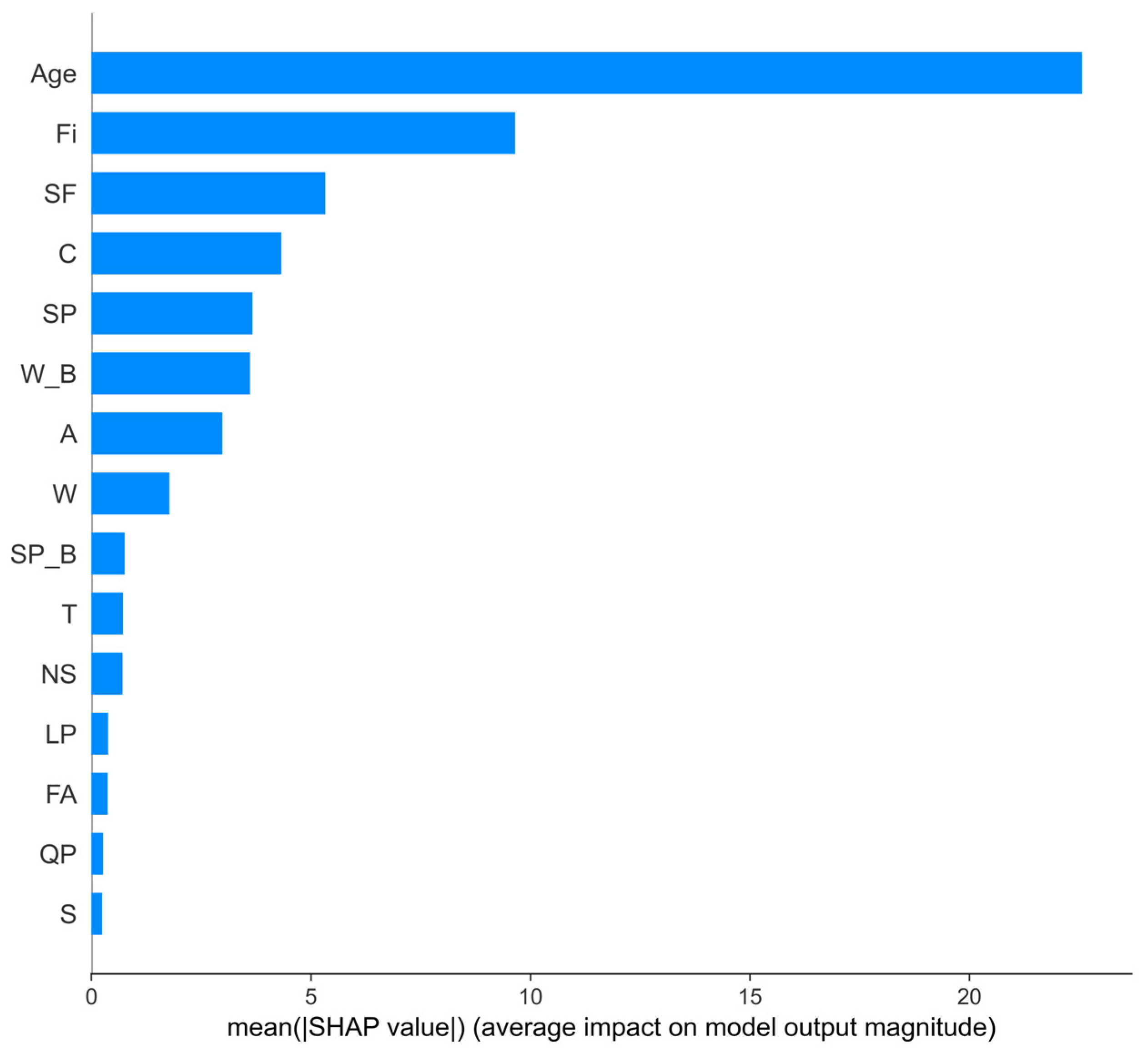
Whereas the preceding subsection elucidated the analysis of feature importance utilizing XGBoost’s built-in feature importance and permutation importance, the SHAP method enables a more profound interpretation of the contribution of each input variable to the model’s prediction results. Specifically, the SHAP method not only provides a global ranking of feature importance but also reveals the direction and magnitude of feature effects at the individual sample level [25]. Compared to the two aforementioned methods, SHAP possesses greater mathematical rigor and enhanced interpretability, enabling it to uncover non-linear relationships and interaction effects. Figure 10 presents the feature importance ranking plot generated by SHAP, where a longer blue bar indicates a greater overall contribution of that feature to the model’s predictions.

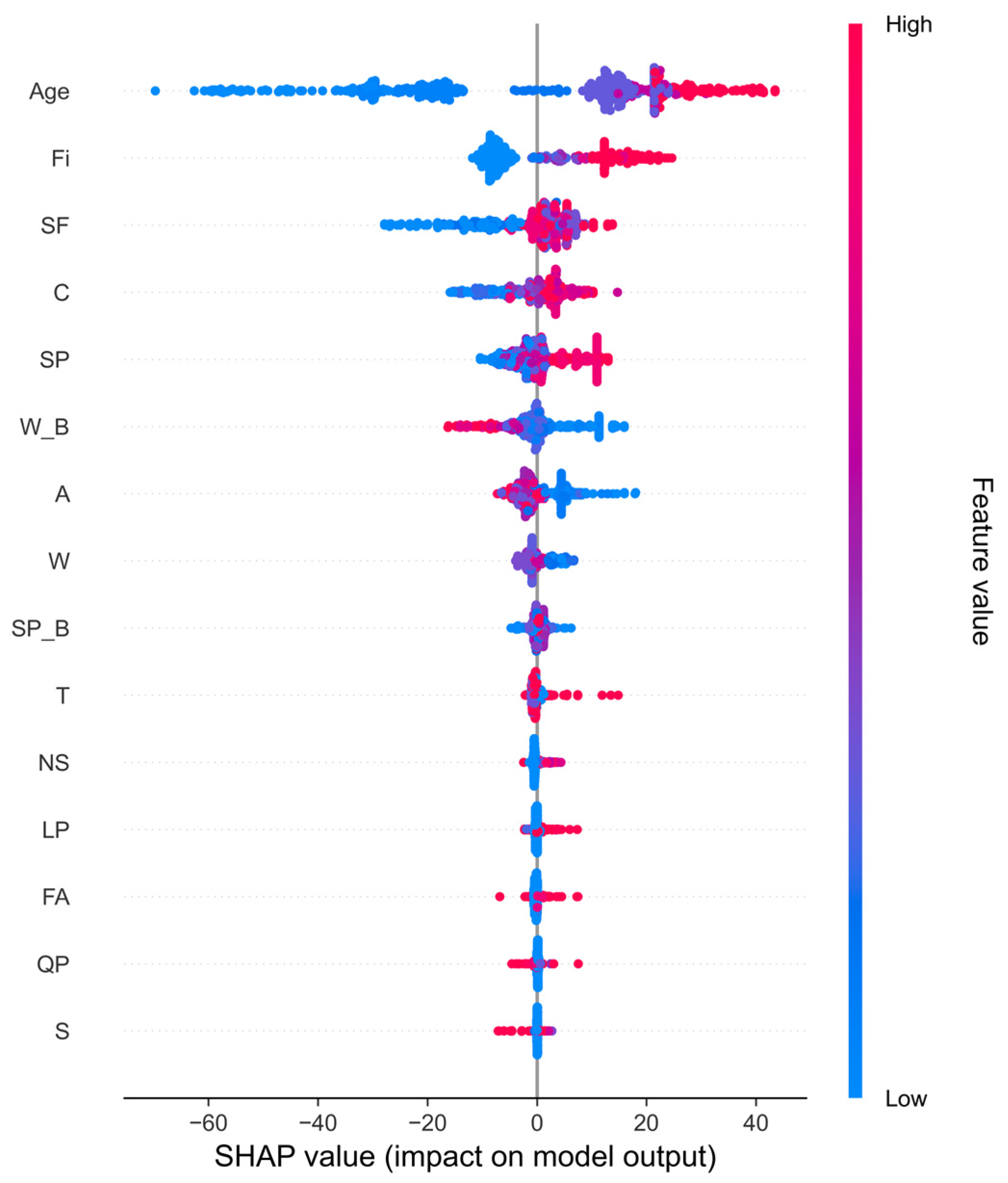
As observed from the figure, Age emerges as the most significant influencing factor among the 15 feature variables. Fi ranks as the second most important factor, followed by SP, SF, and others. This finding aligns closely with the conclusions derived from the previously discussed XGBoost built-in feature importance and permutation importance analyses. Figure 11 presents the SHAP value distribution plot, which calculates the relative importance of each variable using SHAP and ranks them in descending order to determine global feature relevance.

In this plot, the y-axis represents the feature relevance, while the x-axis denotes the SHAP value. The color bar on the right indicates the magnitude of the feature values, where red represents high feature values and blue represents low feature values. The gradient scale ranges from low to high, illustrated by a color transition from blue to red. This figure elucidates how each feature influences the prediction results of the UHPC compressive strength model, revealing the distribution of SHAP values for individual data samples across the various features. As shown in Figure 12, the color transition of the SHAP values for Age from blue to red reveals a clear positive effect on the predicted compressive strength of UHPC, with the maximum SHAP value reaching approximately 45. At early ages, Age makes a negative contribution to the predicted strength, whereas at later ages, it contributes positively and substantially increases the prediction. This observation is consistent with the well-established understanding that longer curing ages allow more sufficient hydration in UHPC, leading to higher compressive strength. Fi also shows a positive contribution to compressive strength, with a maximum SHAP value of approximately 25. This effect can be attributed to the role of fibers in improving the macroscopic mechanical behavior of UHPC through crack bridging, restriction of micro-crack propagation, enhanced matrix confinement, and improved post-peak toughness. Under compressive loading, fibers can delay the coalescence and propagation of micro-cracks to some extent, helping maintain material integrity before failure. This explains why Fi shows high importance in the model. However, the strength enhancement provided by fibers is not unlimited. When the fiber content is too high, non-uniform dispersion, reduced workability, and increased pore defects may occur, which can weaken the reinforcing effect of fibers. Although SF, SP, and T show relatively small SHAP values and thus make limited positive contributions, they still remain relevant factors affecting the predicted compressive strength. In contrast, W/B and A have negative effects on the predicted compressive strength, suggesting that these parameters should be carefully controlled in mixture design to reduce their adverse influence on UHPC strength. By comparison, the SHAP values of C, W, NS, and FA are more closely clustered around zero, indicating that their contributions to the prediction of UHPC compressive strength are relatively limited.

3.5. PDP and ICE Analysis

To further examine how key variables affect the UHPC compressive strength predicted by the XGBoost model, Partial Dependence Plots (PDP) and Individual Conditional Expectation (ICE) curves were used as supplementary interpretation tools. PDP and ICE are model-interpretation methods, and their results describe the response patterns learned by the trained model under the current data distribution. These patterns should not be directly interpreted as the causal effect of a single variable on compressive strength. This point is particularly important for UHPC mixture design, where the input variables are inherently constrained by factors such as W/B, total binder content, aggregate volume fraction, superplasticizer dosage, and absolute volume. As a result, the variables are not fully independent. The PDP and ICE results were therefore interpreted as model response trends and discussed together with the basic material mechanisms and mixture design constraints of UHPC.

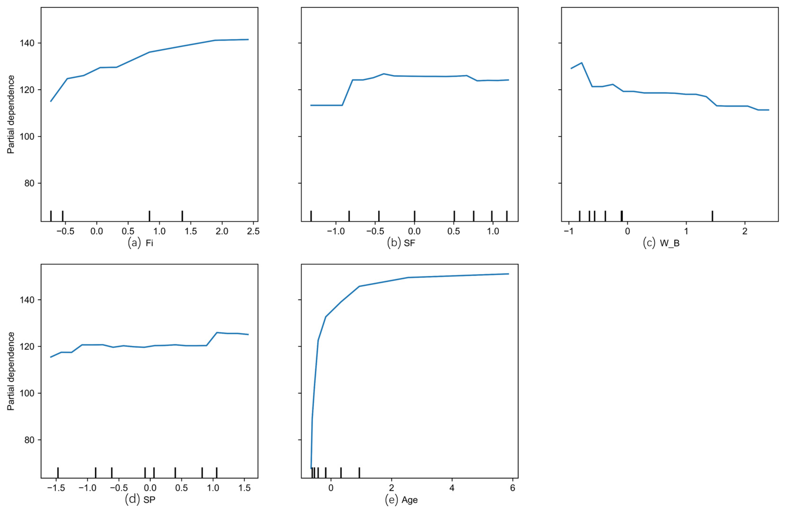
Figure 12 presents the PDP curves for key variables including Fi, SF, W/B, SP, and Age.

As shown in Figure 12, Age has the strongest influence on the model-predicted strength. When Age increases from a low level, the predicted compressive strength rises rapidly, but the growth rate gradually decreases and eventually approaches a plateau. This pattern suggests that the model effectively captures the typical development of UHPC compressive strength with curing age. This behavior can be explained by the rapid hydration and microstructural densification that occur at early ages, which make a major contribution to strength development. At later ages, the rate of strength gain gradually decreases. This trend is consistent with the general hydration process and strength development mechanism of UHPC. For W/B, the PDP curve shows an overall downward trend, suggesting that, within the current data distribution and the patterns learned by the model, a higher water-to-binder ratio generally reduces the predicted compressive strength. This result is consistent with the basic design principle of UHPC, which relies on a low water-to-binder ratio and a dense matrix. A lower W/B helps reduce capillary porosity and enhance matrix density, thereby improving compressive strength. However, based on the aforementioned VIF analysis, W/B exhibits strong multicollinearity with variables such as C, W, and SF. Therefore, this trend should be interpreted as the comprehensive response of variables related to the water-binder proportions, rather than being construed as W/B independently determining the compressive strength. The PDP curve for Fi shows an overall upward trend, suggesting that a higher fiber content generally increases the model-predicted strength. This effect may be related to the role of fibers in improving the compressive failure behavior of UHPC, mainly through crack bridging, micro-crack restraint, and delayed crack propagation, which together enhance its macroscopic compressive performance. For SF, the PDP curve increases in the lower-value range and then gradually levels off. This pattern suggests that an appropriate dosage of silica fume is beneficial for improving the predicted strength, mainly because of its micro-filling effect, pozzolanic activity, and contribution to matrix densification. However, once SF reaches a certain level, further increasing its content yields limited enhancement in the predicted strength, demonstrating that the model has learned the diminishing marginal effect of silica fume. The PDP curve for SP is relatively flat overall, with only a slight increase in the higher-value range. This suggests that the role of superplasticizer in strength prediction is mainly indirect. Rather than acting as an independent factor that directly determines compressive strength, SP may influence the predicted strength by improving workability, facilitating the compaction of low-W/B mixtures, and promoting matrix densification.

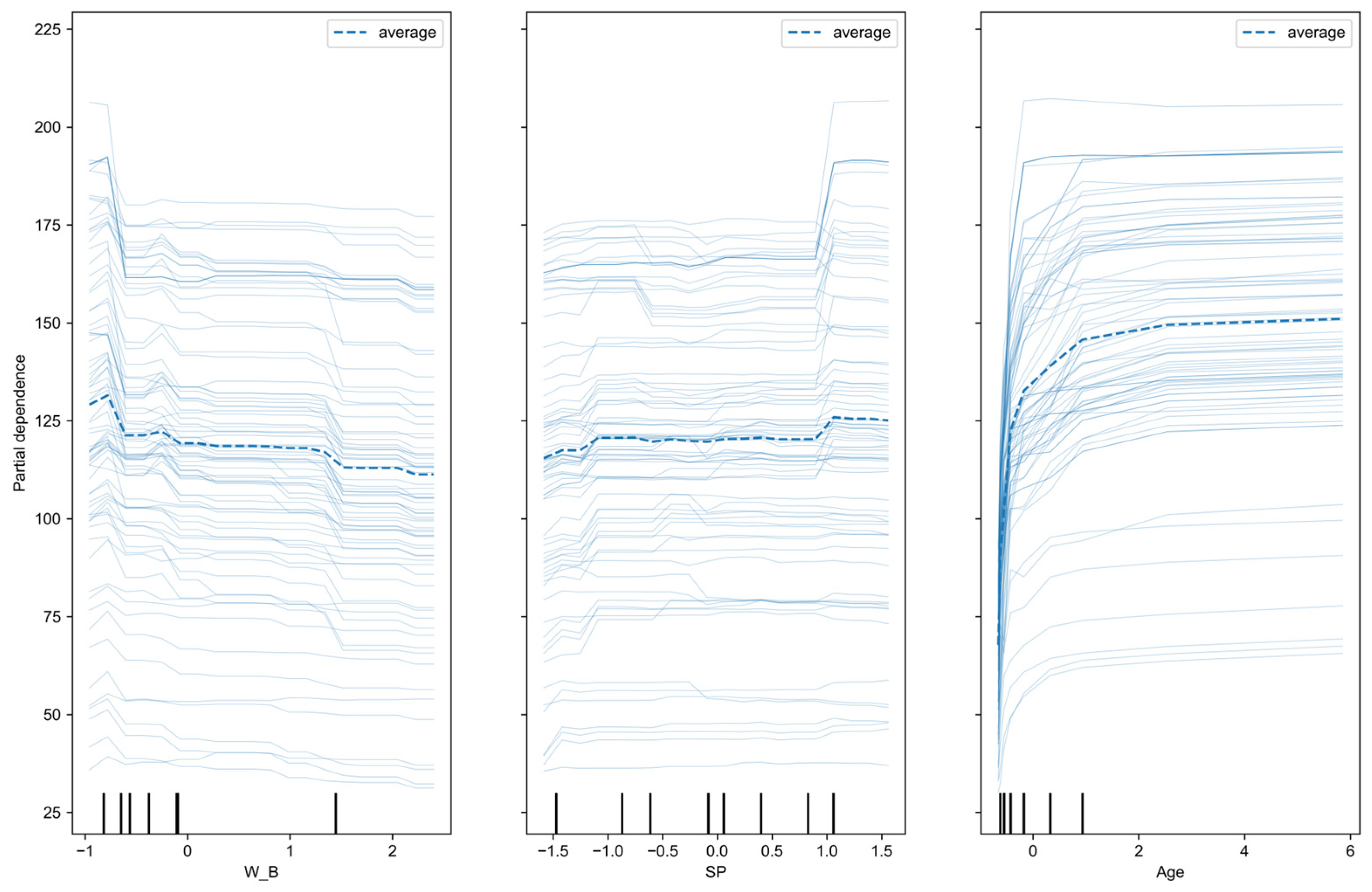
Figure 13 further presents the ICE curves for W/B, SP, and Age. The light-blue solid curves depict the individual ICE profiles, whereas the blue dashed curve represents their average value.

Unlike PDP, which describes the average model response, ICE curves capture sample-level variations in the response to a given variable. As shown in Figure 13, the average ICE curve for W/B shows an overall downward trend, and most individual curves also indicate a decrease in predicted compressive strength as W/B increases. Nevertheless, the curve levels and slopes vary noticeably among samples. This suggests that the effect of W/B on model prediction is not independent, but is influenced by other mixture-related factors, such as binder composition, fiber content, superplasticizer dosage, and curing conditions. For SP, the ICE curves show a relatively flat average trend, with only a slight increase in the higher-value range. However, the individual ICE curves vary considerably, suggesting that the effect of SP on UHPC compressive strength is strongly dependent on the mixture conditions. In some mixtures, an appropriate SP dosage may improve strength indirectly by enhancing particle dispersion and casting quality. In other cases, its effect may be limited by factors such as W/B, powder composition, and total binder content. The ICE curves for Age show a relatively consistent upward trend. The increase is more pronounced at early curing ages and then gradually levels off. This pattern indicates that curing age has a stable effect on the model-predicted strength, with most samples showing higher predicted strength as age increases. This result is consistent with the PDP analysis and further confirms the importance of Age in predicting UHPC compressive strength.

Overall, the PDP and ICE analyses show that Age, W/B, Fi, SF, and SP affect the XGBoost predictions to different extents. Age has a clear positive effect on the predicted compressive strength, whereas W/B generally has a negative effect. Fi and SF contribute positively within certain ranges, while the effect of SP is relatively mild and depends more strongly on the mixture conditions.

3.6. Multi-Objective Optimization Results

3.6.1. Objective Function

After the optimal predictive model was identified, XGBoost was used as the surrogate model for UHPC compressive strength prediction and coupled with NSGA-II for multi-objective optimization. The optimization objectives were to maximize UHPC compressive strength while minimizing material cost and carbon emissions. Because NSGA-II is commonly implemented in a minimization framework, the strength maximization objective was reformulated as the minimization of negative compressive strength. The three objective functions can be expressed as follows:

$$\begin{array}{l} \max f_1(x)=-CS(x)\\ \min f_2(x)={\displaystyle \sum _{i=1}^n\left(m_i\times c_i\right)}\\ \min f_3(x) ={\displaystyle \sum _{i=1}^n\left(m_i\times e_i\right)}\end{array}$$

(11)

where $CS(x)$ denotes the compressive strength of UHPC predicted by the XGBoost model.; $m_i$ represents the amount of the i-th material per unit volume, expressed in kg/m³; $c_i$ denotes the unit price of the i-th material, expressed in USD/kg; $e_i$ denotes the carbon emission factor of the i-th material, expressed in kg CO₂-eq/kg.

Table 5. Carbon emission factors, unit costs, and specific gravities of the raw materials.

Input Parameter	Carbon Emission Factor (kg CO2-eq/kg)	Unit Price (USD/t)	Unit Price Used in Model (USD/kg)	Specific Gravity
C/(kg/m3)	0.855	400	0.4000	3.14
S/(kg/m3)	0.052	45	0.0450	2.90
SF/(kg/m3)	0	800	0.8000	2.20
LP/(kg/m3)	0.008	50	0.0500	2.73
QP/(kg/m3)	0.01	800	0.8000	2.67
FA/(kg/m3)	0.009	20	0.0200	2.70
NS/(kg/m3)	0.0139	5000	5.0000	2.20
A/(kg/m3)	0.004	50	0.0500	2.65
W/(kg/m3)	0.000318	1.0	0.0010	1.00
Fi/(kg/m3)	1.496	1800	1.8000	7.85
SP/(/kg/m3)	0.7200	3400	3.4000	1.05

summarizes the carbon emission factors, unit costs, and specific gravities of the various raw materials, as compiled from the relevant literature [26,27,28,29,30,31,32,33,34,35,36].

Material prices and carbon emission factors can vary with region, production process, transportation distance, and life-cycle boundary. This uncertainty is particularly important for industrial by-products such as silica fume, slag, and fly ash, because different carbon allocation methods may lead to noticeable differences in the calculated results. For this reason, the cost and carbon emission results reported in this study are mainly intended for relative comparison among mixtures within the same calculation framework, rather than as absolute values applicable to all regions and production conditions.

3.6.2. Constraints

The dosages of 11 constituent materials were used as decision variables in the multi-objective optimization, including cement (C), slag (S), silica fume (SF), limestone powder (LP), quartz powder (QP), fly ash (FA), nano-silica (NS), aggregate (A), water (W), fiber (Fi), and superplasticizer (SP). The lower and upper bounds of each variable were defined from the corresponding dosage range in the original dataset to reduce the risk of generating mixtures far outside the available data distribution. To maintain the engineering feasibility of the optimized mixtures, several constraints were imposed in the NSGA-II procedure. The predicted compressive strength of UHPC was required to be no less than 120 MPa. The water-to-binder ratio (W/B) was limited to 0.18–0.25, and the superplasticizer-to-binder ratio (SP/B) was limited to 0–0.08. In addition, the total absolute volume of all constituent materials, calculated from their respective densities, was required to be close to 1 m³, with an allowable deviation of ±10 L/m³. The above constraints can be expressed as follows:

$$\min m_i\le m_i\le \max m_i$$

(12)

$$CS(x)\ge 120 \mathrm{MPa}$$

(13)

$$0\le SP/B\le 0.08$$

(14)

$$0.18\le W/B\le 0.25$$

(15)

$$\left|V(x)-1000\right|\le 10$$

(16)

$$V(x)={\displaystyle \sum _{i=1}^n\frac{m_i}{S{G}_i}}$$

(17)

where $CS(x)$ denotes the compressive strength predicted by the XGBoost model, $V(x)$ represents the sum of the absolute volumes of all constituent materials in a candidate mixture, expressed in L/m³. and $S{G}_i$ denotes the specific gravity of the i-th material. Considering possible numerical uncertainties related to database sources, material density values, and the optimization process, the absolute volume was allowed to vary within 1000 ± 10 L/m³. This constraint helps improve the physical feasibility of the recommended mixture proportions.

In this study, 120 MPa was set as the minimum compressive strength constraint to ensure that the optimized mixtures satisfy the basic strength requirement of UHPC. It should be noted that 120 MPa does not represent the highest performance target for high-grade UHPC, but rather serves as the minimum mechanical performance threshold in the multi-objective optimization process. When material cost and carbon emissions are simultaneously considered as minimization objectives, the optimization algorithm may tend to reduce material consumption, cost, and carbon emissions while satisfying the lower strength limit. Therefore, the recommended mixtures obtained in this study should be interpreted as economical and low-carbon compromise solutions that meet the basic strength requirement, rather than as UHPC mixtures designed to achieve the highest possible strength.

The preceding feature importance and SHAP analyses showed that curing age (Age) plays an important role in predicting the compressive strength of UHPC. However, the multi-objective optimization in this study was intended to obtain recommended UHPC mixture proportions under standard engineering conditions, rather than to optimize the curing regime itself. For this reason, the curing temperature (T) and curing age (Age) were fixed at 20 °C and 28 days, respectively, during the optimization process. This setting represents a typical design scenario for the 28-day compressive strength of UHPC under conventional standard curing conditions. Accordingly, the recommended mixture proportions obtained in this study should be understood as computationally recommended results for the specific condition of 20 °C and 28 days, rather than global optima applicable to all curing temperatures and ages. Future work may include curing temperature and curing age as additional optimization variables to enable coupled optimization of mixture proportions and curing regimes.

3.6.3. TOPSIS Scoring Evaluation

The NSGA-II algorithm inherently yields a series of non-dominated solutions; therefore, to identify and recommend the Best Compromise Solution from this Pareto set, the Technique for Order Preference by Similarity to Ideal Solution (TOPSIS) was employed in this study. This method determines a relative closeness score by calculating the Euclidean distance from each solution to both the Positive Ideal Solution (characterized by maximum compressive strength, minimum material costs, and minimum carbon emissions) and the Negative Ideal Solution. Ultimately, the solution with the highest relative closeness score was selected as the TOPSIS-recommended compromise mixture from the feasible Pareto solutions. This solution should be interpreted as a computationally recommended candidate obtained under the specified objective functions, constraints, and equal-weighting scheme, rather than as an experimentally verified optimal UHPC mix design. Based on the normalized decision matrix, TOPSIS identifies the positive ideal solution and the negative ideal solution among the available alternatives. Subsequently, the distances from each evaluated alternative to the ideal and anti-ideal solutions are calculated to determine the relative closeness of each alternative to the positive ideal solution. This relative closeness serves as the foundation for assessing their relative merits. The specific procedure for the TOPSIS scoring evaluation is detailed as follows:

$$D_i^{+}=\sqrt{{\displaystyle \sum _{j=1}^3(r_{ij}-r_j^{+}}{)}^2}$$

(18)

$$D_i^{-}=\sqrt{{\displaystyle \sum _{j=1}^3(r_{ij}-r_j^{-}}{)}^2}$$

(19)

$$C_i={\displaystyle \frac{D_i^{-}}{D_i^{+}+D_i^{-}}},(0\le C_i\le 1)$$

(20)

In this study, NSGA-II was used for multi-objective optimization of UHPC mixture proportions. The population size, number of generations, and number of offspring per generation were set to 200, 500, and 100, respectively. Real-valued random sampling was adopted for initialization. Simulated binary crossover (SBX) was used as the crossover operator, with a crossover probability of 0.9 and a distribution index of 15, while polynomial mutation (PM) was used as the mutation operator, with a distribution index of 20. To make the results reproducible, the random seed was fixed at 1, and the algorithm was terminated after the prescribed number of generations. The optimization problem involved 11 decision variables, 3 objectives, and 6 inequality constraints. Before TOPSIS-based decision-making, candidate solutions that failed to satisfy the constraints on compressive strength, water-to-binder ratio, superplasticizer-to-binder ratio, or absolute volume were further screened out to ensure the engineering feasibility of the final recommended mixture.

In the baseline analysis, equal weights were assigned to compressive strength, material cost, and carbon emissions, namely:

$$w_{CS}=w_{COST}=w_{C{O}_2}={\displaystyle \frac{1}{3}}$$

(21)

where $w_{CS}$, $w_{COST}$, and $w_{C{O}_2}$ represent the weights assigned to compressive strength, material cost, and carbon emissions, respectively. Equal weighting was adopted because this study aimed to obtain balanced UHPC mixture proportions that simultaneously consider mechanical performance, economic efficiency, and environmental impact, rather than exclusively pursuing the highest compressive strength, the lowest material cost, or the lowest carbon emissions. It should be noted that the TOPSIS-recommended solution is affected by the assigned weights. Therefore, the solution obtained in this study represents a TOPSIS-recommended compromise mixture under the equal-weighting condition. It should be viewed as a computational candidate selected from the feasible Pareto solutions, rather than as an experimentally validated optimal UHPC mix design.

3.6.4. Multi-Objective Optimization Results

Using the trained XGBoost model as the predictive surrogate, NSGA-II was applied to perform tri-objective optimization of UHPC mixture proportions. The optimization objectives were to maximize the 28-day compressive strength while minimizing total material cost and carbon emissions. From the Pareto non-dominated solutions that satisfied the constraints on compressive strength, water-to-binder ratio, superplasticizer-to-binder ratio, and absolute volume, TOPSIS was then used to select the recommended compromise mixture from the feasible Pareto solution set. In this study, total material cost denotes the cost of raw materials required to produce 1 m³ of UHPC, expressed in USD/m³, whereas carbon emissions denote the total emissions associated with producing 1 m³ of UHPC, expressed in kg CO₂-eq/m³.

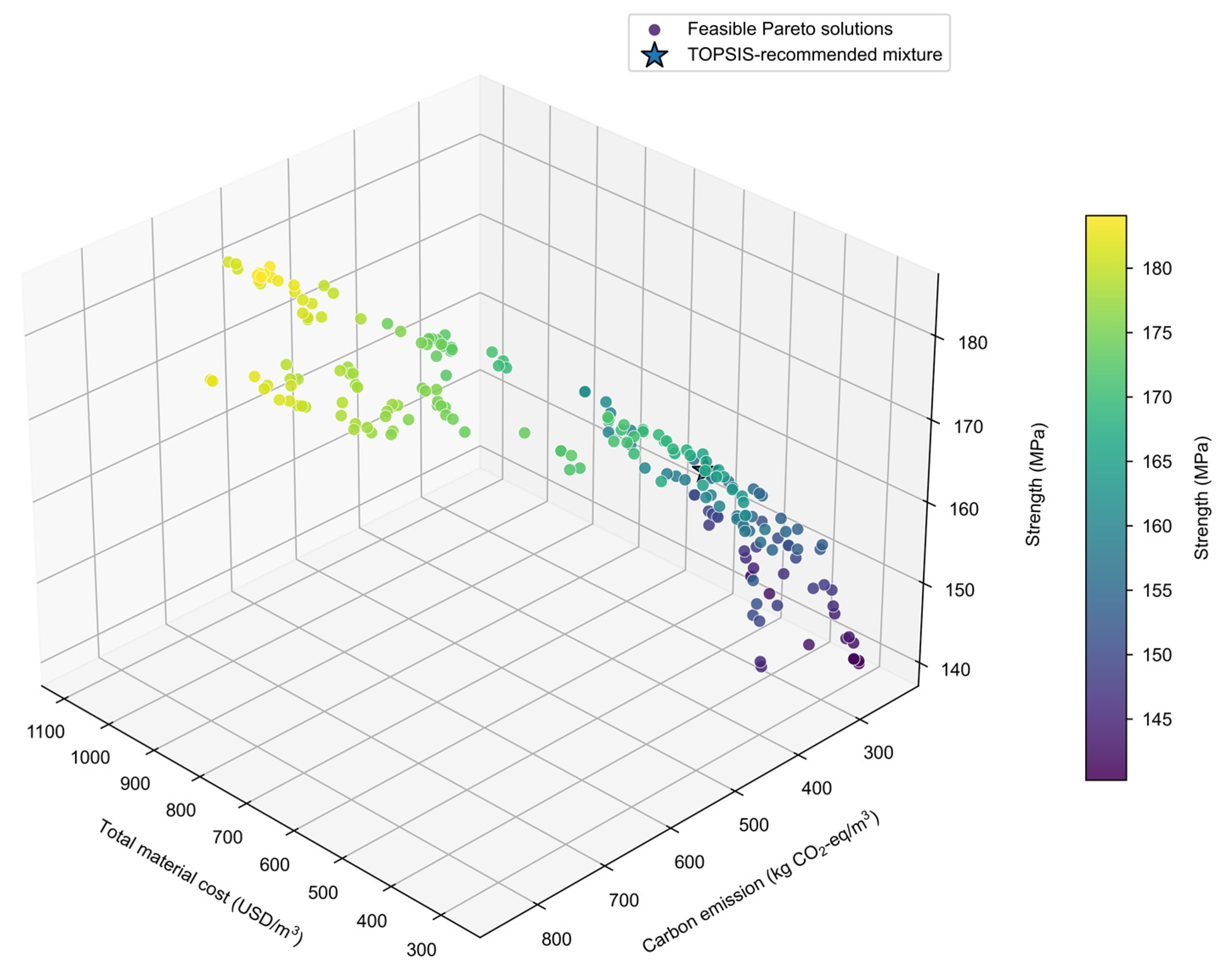
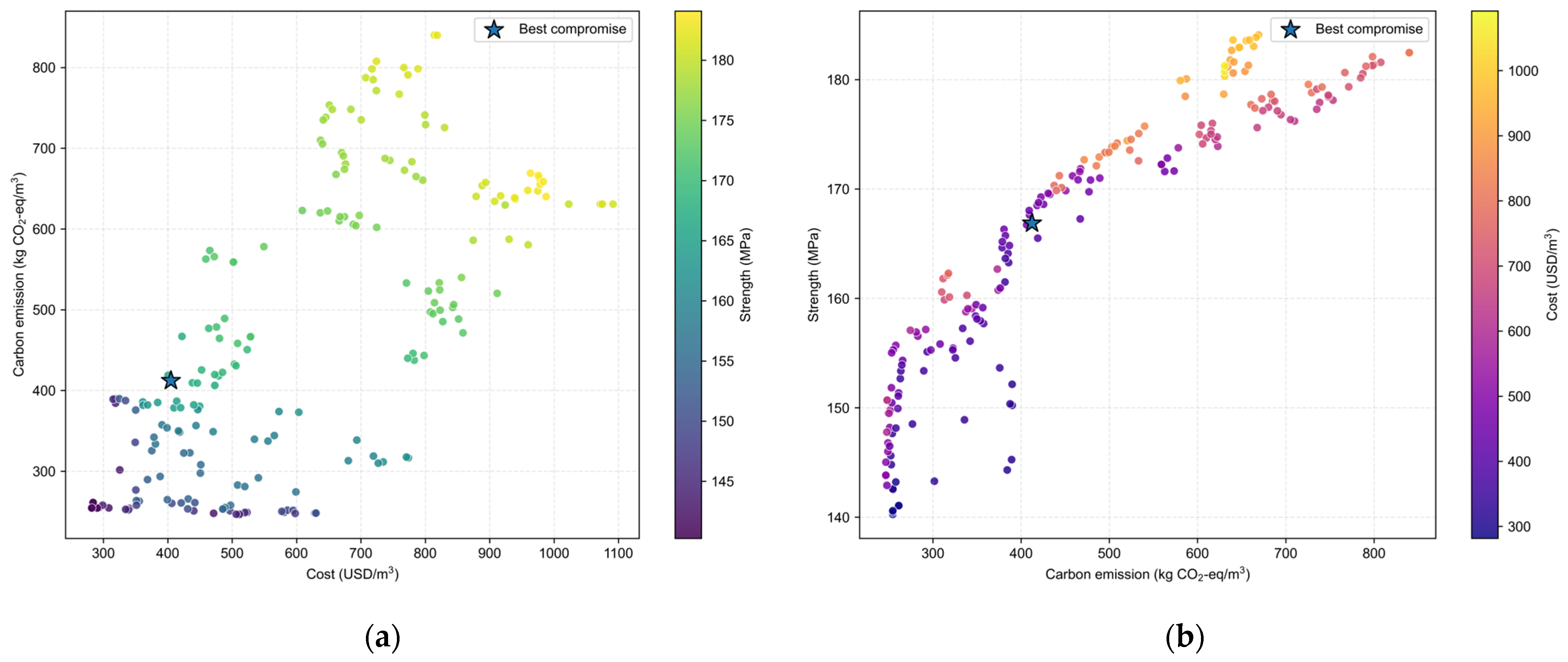
Figure 14 presents the distribution of the Pareto solutions satisfying the engineering constraints in the three-dimensional objective space of compressive strength, total material cost, and carbon emissions.

The Pareto solutions are not clustered in a single region, but are distributed across the objective space, showing a clear trade-off among the three objectives. In general, higher material cost and carbon emissions are associated with higher model-predicted compressive strength. This trend is reasonable because high-strength UHPC often requires larger amounts of binder materials, silica fume, fibers, or other costly constituents, which also increases the associated carbon emissions. By contrast, mixtures with lower cost and lower carbon emissions are more favorable from economic and environmental perspectives, but they usually show lower predicted strength. These results suggest that UHPC mixture optimization should not be driven by a single objective; instead, mechanical performance, economic efficiency, and environmental impact need to be considered together.

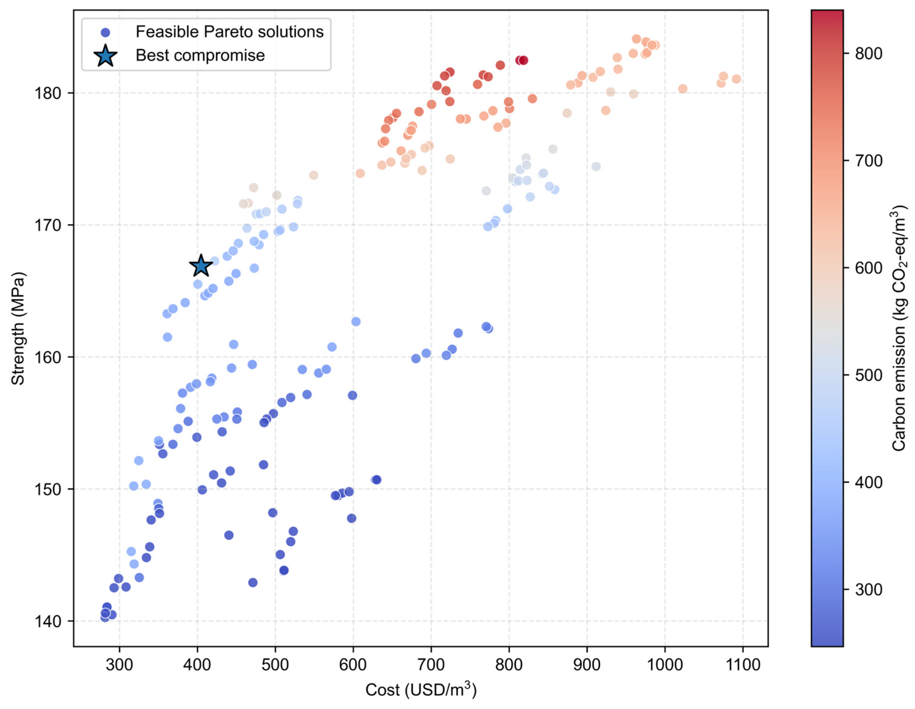
Figure 15 further illustrates the relationship between total material cost and predicted compressive strength, with the color scale representing the carbon emission level.

As shown in the figure, when the total material cost is relatively low, the predicted strength of UHPC is mainly distributed within approximately 140–165 MPa. With increasing material cost, the predicted strength gradually increases and can exceed 180 MPa. However, this improvement is accompanied by clear trade-offs, as the high-strength region generally corresponds to higher carbon emissions. Under the current assumptions for material prices and carbon emission factors, enhancing the compressive strength of UHPC therefore tends to involve higher economic and environmental costs. The TOPSIS-selected compromise solution is not located in the highest-strength region, but instead lies in a balanced region with moderate cost, moderate carbon emissions, and relatively high strength. This suggests that the selected solution better reflects the principle of overall compromise in multi-objective optimization, rather than the pursuit of a single optimum.

Figure 16 further illustrates the relationship among total material cost, carbon emissions, and compressive strength.

The relationship between total material cost and carbon emissions shows that most Pareto solutions follow a similar increasing pattern in both objectives. In other words, mixtures with higher material costs generally tend to have higher carbon emissions. This trend is mainly related to the use of higher binder contents, larger silica fume dosages, fibers, and other high-value constituents in UHPC. However, some candidate mixtures still show noticeable differences in carbon emissions at comparable cost levels, suggesting that carbon emissions can be reduced by adjusting the proportions of different constituent materials without substantially increasing cost. The relationship between carbon emissions and compressive strength further shows that the predicted strength generally increases as carbon emissions rise. However, after the strength reaches a relatively high level, further improvement requires a greater carbon emission penalty. This reflects a marginal increase in environmental cost associated with strength enhancement in UHPC. In practical engineering applications, pursuing the highest possible strength may result in substantial increases in both material cost and carbon emissions, whereas focusing only on minimum cost or minimum carbon emissions may lead to a loss in mechanical performance. For this reason, TOPSIS was used to select the TOPSIS-recommended compromise mixture from the Pareto solution set, providing a recommended mixture that balances strength, economic efficiency, and environmental impact.

The TOPSIS results show that, under the equal-weighting scheme, the TOPSIS-recommended compromise mixture had a predicted compressive strength of about 167 MPa, a total material cost of about 404 USD/m³, and carbon emissions of about 412 kg CO₂-eq/m³. Compared with the highest-strength solution, this mixture reduced both material cost and carbon emissions, while still providing higher strength than the lowest-cost or lowest-carbon-emission solutions. It can therefore be considered a balanced recommended mixture that satisfies the engineering constraints. This mixture is not the single-objective optimum in terms of strength, cost, or carbon emissions within the Pareto solution set; rather, it represents the best compromise obtained by jointly considering compressive strength, material cost, and carbon emissions. The SP/B value of the TOPSIS-recommended mixture is 0.0012, which is relatively low for a UHPC mixture with high powder content. Although this solution satisfies the mathematical constraints of the optimization framework and provides a balanced result in terms of predicted strength, material cost, and carbon emissions, its workability may remain uncertain in practical mixing. This is mainly because fresh-state properties, such as flowability, viscosity, and rheological behavior, were not explicitly included as optimization objectives or constraints. Therefore, the recommended mixture should be regarded as a computational candidate rather than a directly applicable mix design. The superplasticizer dosage may need to be adjusted in subsequent experimental trials to meet practical workability requirements.

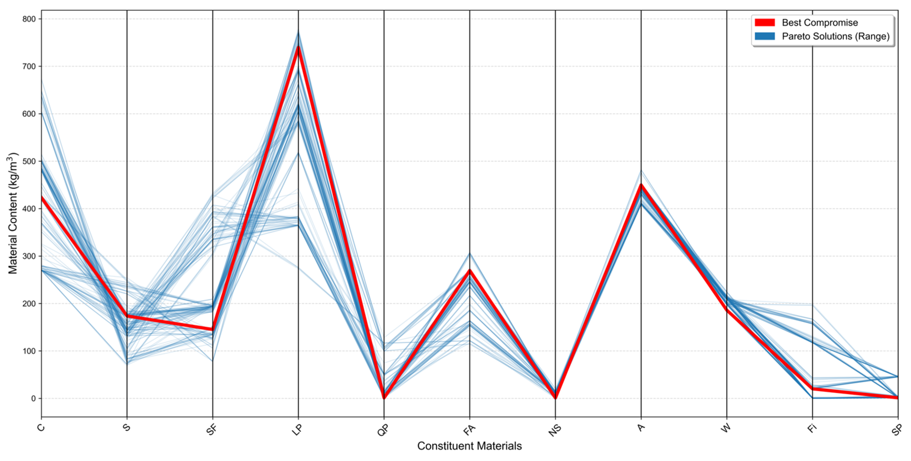
Figure 17 presents the distribution of material compositions for the candidate mixtures in the Pareto solution set, with the TOPSIS-recommended mixture highlighted by the red curve.

As shown in the figure, the Pareto solutions differ noticeably in the dosages of cement, slag, silica fume, limestone powder, fly ash, aggregate, water, and fiber. This suggests that, within the prescribed variable bounds and engineering constraints, NSGA-II was able to identify a range of feasible mixture combinations rather than converging to a single compositional pattern. The TOPSIS-recommended mixture is generally characterized by a moderate cement content, certain amounts of slag and silica fume, a relatively high limestone powder content, an appropriate fly ash dosage, aggregate and water contents within the feasible range, and relatively low dosages of fiber, nano-silica, and superplasticizer. These features indicate that the TOPSIS-recommended compromise mixture does not rely on a large increase in high-cost constituents to achieve the highest possible strength. Instead, it balances strength, material cost, and carbon emissions by adjusting the proportions of binder materials, fillers, and aggregate while still satisfying the strength constraint.

From the viewpoint of mixture design, the relatively high content of limestone powder mainly provides a filling effect and improves particle packing, helping to maintain matrix compactness while reducing the demand for high-carbon and high-cost binder materials. A proper dosage of silica fume can further refine the UHPC matrix through its micro-filling effect and pozzolanic activity. The use of fly ash and slag also helps reduce cement consumption, which is beneficial for both cost reduction and carbon mitigation. Although fibers contribute to crack control and improve the toughness of UHPC under compressive failure, they also make relatively large contributions to material cost and carbon emissions. For this reason, the fiber content in the TOPSIS-recommended mixture remains at a relatively low level. This result reflects the compromise reached by the multi-objective optimization among material performance, cost, and carbon emissions.

The recommended mixture proportion proposed in this study should be regarded as a computational outcome based on the machine-learning surrogate model, assumed material prices, carbon emission factors, and the specified constraints. Since material prices and carbon emission factors can vary with region, transportation distance, procurement scale, and life-cycle assessment boundary, the optimization results are mainly suitable for relative comparison among UHPC mixtures within the same parameter framework. Although the XGBoost model showed good performance on the test set and in the robustness validation, its predictions cannot fully replace experimental testing. Therefore, the TOPSIS-recommended mixture is better viewed as a candidate scheme for subsequent experimental verification and engineering mixture design. Before practical application, further tests on workability, compressive strength, durability, and construction performance are still needed.

Table 6. Comparison with Literature-Reported UHPC Mixtures.

Source	C/kg·m−3	SF/kg·m−3	LP/kg·m−3	FA/kg·m−3	S/kg·m−3	W/kg·m−3	CS/MPa	Carbon Emissions/CO2-eq·m−3
Li et al. [37] M60	448.1	49.8	665.5	— *	—	233.7		—
Li et al. [37] 50 vol% L	560	—	high-volume LP	—	—	—	153	474 kg
this study	423.34	145.25	739.69	269.62	173.73	185.92	166.87	412.22 kg

* “—" indicates that the corresponding material was either not used in the reference study or not reported in the same form. The strength reported by Li et al. is an experimental value, whereas the strength reported in this study is predicted by the XGBoost surrogate model. This comparison is therefore intended mainly to show that the recommended mixture proposed in this study falls within a reasonable range relative to existing studies on UHPC with high-volume limestone powder, rather than to replace subsequent experimental validation.

further assesses the rationality of the TOPSIS-recommended mixture proposed in this study, it was compared with the sustainable UHPC containing a high volume of limestone powder reported by Li et al. [37]. In their study, Li et al. aimed to reduce cement consumption, carbon emissions, and material cost in UHPC, and systematically investigated the effects of replacing binder materials with limestone powder on workability, hydration process, pore structure, compressive strength, shrinkage, carbon emissions, and cost. Limestone powder replacement levels ranging from 0 to 80 vol% were considered. Their results suggested that incorporating a high volume of limestone powder can be an effective approach to reducing the environmental burden and material cost of UHPC.

In terms of mixture composition, the M60 mixture reported by Li et al. contained 448.1 kg/m³ cement, 49.8 kg/m³ microsilica, 665.5 kg/m³ limestone powder, and 233.7 kg/m³ water. In comparison, the TOPSIS-recommended mixture in this study contained 423.34 kg/m³ cement, 145.25 kg/m³ silica fume, 739.69 kg/m³ limestone powder, and 185.92 kg/m³ water. Both mixtures are characterized by relatively low cement content and high limestone powder content, suggesting that the recommended mixture in this study is consistent with the design concept of existing UHPC studies incorporating high-volume limestone powder.

In terms of performance, Li et al. reported that the M40 mixture achieved a 28-day compressive strength of 159.5 MPa. After considering both strength and binder efficiency, they recommended 50 vol% limestone powder as a relatively suitable replacement level, corresponding to a compressive strength of about 153 MPa and an approximately 47% reduction in embodied CO₂ emissions. In this study, the TOPSIS-recommended mixture showed a predicted compressive strength of 166.87 MPa and carbon emissions of 412.22 kg CO₂-eq/m³. These results suggest that both the strength level and low-carbon potential of the recommended mixture fall within a reasonable range compared with existing studies on UHPC containing high-volume limestone powder.

It should also be emphasized that the results reported by Li et al. were obtained from experimental tests, whereas the recommended mixture in this study was derived from a machine-learning surrogate model coupled with NSGA-II/TOPSIS multi-objective optimization. The two studies are not fully identical in terms of raw material system, curing regime, testing conditions, or carbon emission calculation boundary. Therefore, this comparison is mainly intended to support the rationality of the recommended mixture in terms of material composition and performance level, rather than to replace further experimental validation. Additional tests on flowability, compressive strength, durability, and volume stability are still needed for the proposed mixture.

4. Conclusions and Limitations

In this study, machine learning models, including RF, ANN, GBDT, and XGBoost, were developed based on 810 UHPC experimental datasets to predict the compressive strength of UHPC. In addition, SHAP, PDP/ICE, and multi-objective optimization methods were employed to analyze the influence mechanisms of UHPC mixture proportions and to obtain low-carbon and cost-effective recommended mixtures. The main conclusions are as follows:

• The predictive performance of different machine learning models for UHPC compressive strength varied noticeably. Compared with benchmark models such as linear regression, decision tree, and SVR, ensemble learning models, including RF, GBDT, and XGBoost, were better able to capture the complex nonlinear relationship between UHPC mixture parameters and compressive strength. Among them, XGBoost achieved high prediction accuracy and stability in the test-set evaluation, repeated cross-validation, and random-split sensitivity analysis, indicating good generalization ability. Therefore, XGBoost was selected as the surrogate model for the subsequent interpretability analysis and multi-objective optimization;
• The SHAP, feature importance, and PDP/ICE analyses show that variables such as Age, W/B, SF, Fi, and SP play important roles in the prediction results of the XGBoost model. Among these variables, Age has a strong positive effect on the predicted compressive strength, whereas W/B generally shows a negative effect. Within certain ranges, SF and Fi also contribute to an increase in the predicted strength;
• Based on the XGBoost surrogate model and the NSGA-II/TOPSIS framework, a recommended UHPC mixture satisfying the constraints on strength, W/B, SP/B, and absolute volume was obtained. Under the equal-weighting scheme, the TOPSIS-selected TOPSIS-recommended compromise mixture had a predicted compressive strength of 166.87 MPa, a total material cost of 404.67 USD/m³, carbon emissions of 412.22 kg CO₂-eq/m³, a W/B of 0.1835, an SP/B of 0.0012, and an absolute volume of 991.76 L/m³.

Although this study developed an integrated framework for UHPC compressive strength prediction, model interpretation, and multi-objective optimization, and obtained a recommended mixture satisfying the engineering constraints, several limitations remain:

• The database used in this study was collected from published literature and experimental data. Differences among data sources may exist in raw material properties, curing regimes, specimen dimensions, and testing methods. Although data preprocessing, repeated cross-validation, and random-split sensitivity analysis were used to improve the reliability of model evaluation, data heterogeneity may still affect the stability and generalization ability of the model predictions;
• The multi-objective optimization in this study mainly considered compressive strength, material cost, and carbon emissions. In practical engineering applications, UHPC performance is also affected by workability, setting time, shrinkage, tensile performance, flexural performance, and durability. Since these performance indicators were not complete in the original database, they were not fully incorporated into the optimization objectives or constraints. Future studies may further conduct multi-performance collaborative optimization after supplementing the database with additional experimental results;
• The calculation of material cost and carbon emissions was based on unified material prices and carbon emission factors, and was mainly intended for relative comparison among different mixtures within the same optimization framework. In real engineering practice, material prices and carbon emission factors can vary with region, transportation distance, procurement scale, production process, and life-cycle assessment boundary. Future work may therefore incorporate region-specific price data and life-cycle assessment data to perform sensitivity analysis on cost and carbon emission results;
• The TOPSIS-recommended mixture has not yet been validated through actual mixing and experimental testing. Further studies should experimentally evaluate the recommended mixture in terms of workability, 28-day compressive strength, durability, and volume stability, and compare the measured results with the model predictions. Such validation would help further refine and improve the UHPC mixture optimization framework.

References

1. Nie, J.; Li, C.; Qian, G.; Pan, R.; Fei, B.; Deng, S. Effect of shape and content of steel fiber on workability and mechanical properties of Ultra-High Performance Concrete UHPC. Mater. Rep. 2021, 35, 04042–04052. [Google Scholar]
2. Tian, J.; Yan, J.; Wang, X.; Zhao, Y.; Shi, Q. Prediction of load-bearing capacity of steel plate-RC composite coupling beam based on PSO-SVR algorithm. J. Vib. Shock 2025, 44, 155–162. [Google Scholar] [CrossRef]
3. Deng, F.; He, Y.; Zhou, S.; Yu, Y.; Cheng, H.; Wu, X. Compressive strength prediction of recycled concrete based on deep learning. Constr. Build. Mater. 2018, 175, 562–569. [Google Scholar] [CrossRef] [Scilit]
4. Mahmood, M.S.; Elahi, A.; Zaid, O.; Alashker, Y.; Șerbănoiu, A.A.; Grădinaru, C.M.; Ullah, K.; Ali, T. Enhancing compressive strength prediction in self-compacting concrete using machine learning and deep learning techniques with incorporation of rice husk ash and marble powder. Case Stud. Constr. Mater. 2023, 19, e02557. [Google Scholar] [CrossRef] [Scilit]
5. Zhou, S.; Jia, Y.; Li, K.; Li, Z.; Wu, X.; Peng, H.; Zhang, C.; Han, K.; Wang, C. Mix proportion optimization of ultra-high performance concrete based on machine learning. J. Tongji Univ. (Nat. Sci.) 2024, 52, 1018–1023. [Google Scholar]
6. Bolbolvand, M.; Tavakkoli, S.M.; Alaee, F.J. Prediction of compressive and flexural strengths of ultra-high-performance concrete (UHPC) using machine learning for various fiber types. Constr. Build. Mater. 2025, 493, 143135. [Google Scholar] [CrossRef] [Scilit]
7. Gu, J.; Zhang, Z.; Liu, X.; Chang, B.; Zhao, T. Application of data-driven machine learning in performance prediction and multi-objective optimization of green sustainable steam-cured concrete. Sustain. Chem. Pharm. 2026, 50, 102336. [Google Scholar]
8. Kashem, A.; Karim, R.; Malo, S.C.; Das, P. Ultra-High-Performance Concrete (UHPC); Mendeley Data: London, UK, 2023; Volume 20, p. e02991. [Google Scholar] [CrossRef]
9. Yuan, Z.; Hu, Y.; Yang, Y. Modeling Towards Freeway Real-time Traffic Crash PredictionConsidering Multi-dimensional Dynamic Feature Interactions. J. Transp. Syst. Eng. Inf. Technol. 2022, 22, 215–223. [Google Scholar] [CrossRef]
10. Cao, Y. Investigation into the prediction of concrete compressive strength using a bayesian-optimized CatBoost model. Concrete 2025, 7, 87–94. [Google Scholar]
11. Sobuz, M.H.R.; Alzlfawi, A.; Hakeem, I.Y.; Tilak, M.K.C.; Kabbo, M.K.I.; Jameel, M.; Abubakar, S.A. Machine learning-based modeling to predict and parametrically optimize the compressive strength of nanomaterial concrete composites exposed to elevated temperatures. Case Stud. Constr. Mater. 2025, 23, e05546. [Google Scholar] [CrossRef] [Scilit]
12. Zhang, J.; Guo, W.; Song, B.; Zhuo, Y.; Zhang, Y. Performance prediction of asphalt pavement based on random forest. J. Beijing Univ. Technol. 2021, 47, 1256–1263. [Google Scholar]
13. Abbas, M.M.; Muntean, R. Predictive modelling of concrete tensile strength using ANN and Supplementary Cementitious Materials (SCMs). Constr. Build. Mater. 2025, 489, 142362. [Google Scholar] [CrossRef] [Scilit]
14. Song, Q.; Xu, S.; Lu, Y.; Niu, D.; Xia, J.; Zhao, H.; Lv, Y.; Bao, J.; Xue, S.; Li, R. Study on the characteristics and prediction of concrete carbon emissions based on a machine learning approach with spatiotemporal heterogeneity analysis. Case Stud. Constr. Mater. 2025, 23, e05410. [Google Scholar] [CrossRef] [Scilit]
15. Alizamir, M.; Wang, M.; Ikram, R.M.A.; Gholampour, A.; Ahmed, K.O.; Heddam, S.; Kim, S. An Interpretable XGBoost-SHAP Machine Learning Model for Reliable Prediction of Mechanical Properties in Waste Foundry Sand-Based Eco-Friendly Concrete. Results Eng. 2025, 25, 104307. [Google Scholar] [CrossRef] [Scilit]
16. Xu, J.; Hou, X.; Wu, X.; Liu, Y.; Sun, G. Slope Displacement Prediction Using the MIC-XGBoost-LSTM Model. China J. Highw. Transp. 2024, 37, 38–48. [Google Scholar] [CrossRef]
17. Kazemi, F.; Shafighfard, T.; Jankowski, R.; Yoo, D.-Y. Active learning on stacked machine learning techniques for predicting compressive strength of alkali-activated ultra-high-performance concrete. Arch. Civ. Mech. Eng. 2024, 25, 24. [Google Scholar] [CrossRef] [Scilit]
18. Padarian, J.; McBratney, A.; Minasny, B. Game theory interpretation of digital soil mapping convolutional neural networks. SOIL 2020, 6, 389–397. [Google Scholar] [CrossRef] [Scilit]
19. Lundberg, S.M.; Lee, S.-I. A unified approach to interpreting model predictions. Adv. Neural Inf. Process. Syst. 2017, 30, 4768–4777. [Google Scholar]
20. Ekanayake, I.; Meddage, D.; Rathnayake, U. A novel approach to explain the black-box nature of machine learning in compressive strength predictions of concrete using Shapley additive explanations (SHAP). Case Stud. Constr. Mater. 2022, 16, e01059. [Google Scholar] [CrossRef] [Scilit]
21. Raihan, M.; Khan, M.; Kee, S.; Nahid, A.A. Detection of the chronic kidney disease using XGBoost classifier and explaining the influence of the attributes on the model using SHAP. Sci. Rep. 2023, 13, 6263. [Google Scholar] [CrossRef] [Scilit] [PubMed]
22. Wang, J.; Wang, X.; Li, Y.; Ye, A. Machine Learning Prediction and Interpretability Comparison for Seismic Response Analysis of Small-to-medium Span Conventional Continuous Girder Bridges. China J. Highw. Transp. 2025, 38, 61–74. [Google Scholar] [CrossRef]
23. Wang, Z.; Wang, Z.; Li, Z.; Miao, P.; Wu, L. Prediction of sandy soil liquefaction based on machine learning-GridSearchCV. J. Vib. Shock 2024, 43, 82–93. [Google Scholar] [CrossRef]
24. Philip, S.; Marakkath, N. Compressive strength prediction and feature analysis for GGBS-Based geopolymer concrete using optimized XGBoost and SHAP: A comparative study of optimization algorithms and experimental validation. J. Build. Eng. 2025, 108, 112879. [Google Scholar] [CrossRef] [Scilit]
25. Chen, Y.; Zhu, J.; Tian, Y.; Ouyang, Z.-H.; Long, J. Analysis of Factors Contributing to Traffic Accident Severity Based on an Integrated Framework of K-Means-XGBoost-SHAP. China J. Highw. Transp. 2025, 38, 209–223. [Google Scholar] [CrossRef]
26. Van den Heede, P.; De Belie, N. Environmental impact and life cycle assessment (LCA) of traditional and ‘green’concretes: Literature review and theoretical calculations. Cem. Concr. Compos. 2012, 34, 431–442. [Google Scholar] [CrossRef] [Scilit]
27. Zhao, J.; Wang, A.; Zhu, Y.; Dai, J.-G.; Xu, Q.; Liu, K.; Hao, F.; Sun, D. Manufacturing ultra-high performance geopolymer concrete (UHPGC) with activated coal gangue for both binder and aggregate. Compos. Part. B Eng. 2024, 284, 111723. [Google Scholar] [CrossRef] [Scilit]
28. Shi, Y.; Long, G.; Ma, C.; Xie, Y.; He, J. Design and preparation of ultra-high performance concrete with low environmental impact. J. Clean. Prod. 2019, 214, 633–643. [Google Scholar] [CrossRef] [Scilit]
29. Chiaia, B.; Fantilli, A.P.; Guerini, A.; Volpatti, G.; Zampini, D. Eco-mechanical index for structural concrete. Constr. Build. Mater. 2014, 67, 386–392. [Google Scholar] [CrossRef] [Scilit]
30. Li, L.; Shao, X.; Ling, T.-C. Life cycle assessment of coal gangue composite cements: From sole OPC towards low-carbon quaternary binder. J. Clean. Prod. 2023, 414, 137674. [Google Scholar] [CrossRef] [Scilit]
31. Müller, H.S.; Haist, M.; Vogel, M. Assessment of the sustainability potential of concrete and concrete structures considering their environmental impact, performance and lifetime. Constr. Build. Mater. 2014, 67, 321–337. [Google Scholar] [CrossRef] [Scilit]
32. Amitani, A.; Miller, S.A. Material performance, economic feasibility, and greenhouse gas emissions of natural pozzolans in concrete: A review and meta-analysis. Resour. Conserv. Recycl. 2026, 228, 108769. [Google Scholar] [CrossRef] [Scilit]
33. Alsalman, A.; Assi, L.N.; Kareem, R.S.; Carter, K.; Ziehl, P. Energy and CO2 emission assessments of alkali-activated concrete and Ordinary Portland Cement concrete: A comparative analysis of different grades of concrete. Clean. Environ. Syst. 2021, 3, 100047. [Google Scholar] [CrossRef] [Scilit]
34. Gu, Y.; Fan, R.; Li, Y.; Zhao, J.; Song, Z.; Chu, H. Multi-Objective Optimization for Nano-Silica-Modified Concrete Based on Explainable Machine Learning. Nanomaterials 2025, 15, 1423. [Google Scholar] [CrossRef] [Scilit] [PubMed]
35. Phan, T.D.; Noh, H.W.; Lee, S.Y.; Kim, D.J. Effects of high-volume limestone powder substitution on hydration and mechanical–microstructural development of low-carbon cement pastes: Simulation and experiment. Constr. Build. Mater. 2025, 471, 140710. [Google Scholar] [CrossRef] [Scilit]
36. Wakjira, T.G.; Kutty, A.A.; Alam, M.S. A novel framework for developing environmentally sustainable and cost-effective ultra-high-performance concrete (UHPC) using advanced machine learning and multi-objective optimization techniques. Constr. Build. Mater. 2024, 416, 135114. [Google Scholar] [CrossRef] [Scilit]
37. Li, P.P.; Brouwers, H.; Chen, W.; Yu, Q. Optimization and characterization of high-volume limestone powder in sustainable ultra-high performance concrete. Constr. Build. Mater. 2020, 242, 118112. [Google Scholar] [CrossRef] [Scilit]
Figure 1. Distribution of input variables and their relationships with compressive strength.
Applsci 16 07093 g001
Figure 2. Pearson and Spearman correlation matrices of input variables.
Applsci 16 07093 g002
Figure 3. VIF analysis of input variables.
Applsci 16 07093 g003
Figure 4. Relationship between predicted and actual values for single models and their relative errors. (a) RF; (b) XGBoost; (c) ANN; (d) GBDT.
Applsci 16 07093 g004
Figure 5. Scatter plots of the prediction results on the testing set for the machine learning models: (a) RF; (b) XGBoost; (c) ANN; (d) GBDT.
Applsci 16 07093 g005aApplsci 16 07093 g005b
Figure 6. Results of the repeated 10-fold cross-validation.
Applsci 16 07093 g006
Figure 7. Sensitivity analysis of model performance under different random seed partitions.
Applsci 16 07093 g007
Figure 8. Built-in feature importance of the XGBoost model.
Applsci 16 07093 g008
Figure 9. Permutation Importance.
Applsci 16 07093 g009
Figure 10. SHAP Feature Importance.
Applsci 16 07093 g010
Figure 11. SHAP Value.
Applsci 16 07093 g011
Figure 12. Partial Dependence Plot (PDP). (a) Fi; (b) SF; (c) W/B; (d) SP; (e) Age.
Applsci 16 07093 g012
Figure 13. ICE curves for W/B, SP, and Age.
Applsci 16 07093 g013
Figure 14. 3D Pareto Front Surface for Multi-Objective Optimization.
Applsci 16 07093 g014
Figure 15. Relationship between total material cost and compressive strength.
Applsci 16 07093 g015
Figure 16. Relationship among total material cost, carbon emissions, and compressive strength: (a) Relationship between total material cost and carbon emissions; (b) Relationship between carbon emissions and compressive strength.
Applsci 16 07093 g016
Figure 17. Parallel Coordinate Plot of All Pareto Solutions.
Applsci 16 07093 g017