Physically Constrained and Location-Aware Machine Learning for Joint Prediction of Clay Compression and Recompression Indices

Abstract

Compression index (Cc) and recompression index (Cur) are essential parameters in one-dimensional consolidation and settlement analysis, yet their direct determination from oedometer testing is time-consuming, costly, and often limited by sparse recompression data. This study develops an interpretable and physically constrained machine-learning framework for the joint prediction of Cc and Cur from four routinely measured index properties: liquid limit (LL), plasticity index (PI), initial void ratio (e), and natural water content (w). A curated subset of 459 natural clay records from the global CLAY/Cc/6/6203 database was used to benchmark single-output and multi-output Random Forest, gradient-boosted tree, and deep neural network models. In addition to conventional random train–test and cross-validation protocols, a leave-one-location-out validation was introduced to evaluate transferability across 81 Country–Location groups. Under the random-split setting, Cc was predicted with moderate-to-good accuracy, with baseline models achieving test R² values of approximately 0.61–0.70 and a geotechnically enriched Random Forest model increasing the test R² to 0.777. Cur was more difficult to predict. Although feature enrichment improved its test R² to 0.507, location-aware validation reduced Cur performance substantially, confirming its stronger dependence on site-specific stress history, fabric, and geological structure. SHAP interpretation identified e and w as the dominant controls on Cc, while Cur exhibited weaker and more diffuse dependence on the available index properties. A physically constrained target transformation based on the bounded ratio of Cur/Cc guaranteed mechanically admissible predictions with Cur < Cc, but did not fully recover the missing information needed for accurate Cur estimation. The proposed constraint is not a governing-equation-based physics-informed model. Rather, it is a mechanically constrained target transformation that preserves the admissible relationship Cur < Cc. The results show that routine index properties can support the useful preliminary prediction of Cc, whereas Cur should be treated as a screening-level estimate unless explicit stress history descriptors are available.

1. Introduction

Settlement and long-term subsidence in soft clay deposits remain major concerns in geotechnical engineering because the serviceability of foundations, embankments, retaining structures, and urban infrastructure is strongly governed by the compressibility of cohesive soils [1,2,3]. In one-dimensional consolidation analysis, this behaviour is commonly represented by the compression index, Cc, which describes virgin compression, and the recompression index, Cur, which represents unloading–reloading stiffness in the overconsolidated range [1,2,3]. Reliable estimation of both parameters is, therefore, essential for settlement assessment, particularly in coastal plains, deltaic deposits, and urbanised soft-clay formations.

Direct determination of Cc and Cur requires oedometer or incremental loading consolidation tests, which are reliable but time-consuming, labour-intensive, and sensitive to sample quality, disturbance, and testing procedures [1,3]. In routine site investigations, index properties such as liquid limit (LL), plasticity index (PI), natural water content (w), and initial void ratio (e) are usually measured more frequently than consolidation parameters [2,3,4]. This has led to widespread use of empirical correlations for estimating Cc, and to a lesser extent Cur, from routine index properties. However, existing correlations, which often use linear or log-linear relationships with LL, PI, or e, or assume Cur as a fixed fraction of Cc, commonly show substantial scatter, limited regional transferability, and limited ability to capture nonlinear interactions between soil state, plasticity, and fabric [4,5,6,7]. This limitation is especially relevant for Cur, which is less directly constrained by routine index properties because it is strongly affected by stress history, overconsolidation, bonding, fabric, and microstructure [3].

Recent advances in machine learning (ML), together with larger geotechnical databases, provide new opportunities for predicting soil parameters from routinely measured properties [7,8,9,10,11,12,13,14,15,16,17]. Tree-based ensemble models, such as Random Forest (RF) and gradient-boosted trees, are well-suited to heterogeneous tabular geotechnical data because they can capture nonlinear relationships and variable interactions without requiring a predefined functional form [18,19]. Deep neural networks (DNNs) offer greater representational flexibility, but they require careful calibration and may be less transparent, particularly for small or noisy datasets [20,21,22]. To improve interpretability, model-agnostic tools such as SHAP can be used to quantify feature contributions and assess whether learned relationships are consistent with geotechnical understanding [16,20,22]. In parallel, physics-informed and data-driven learning approaches have highlighted the importance of combining numerical accuracy with physical consistency, interpretability, and robust validation. In this study, the physical component is, therefore, introduced as a mechanically constrained target transformation, rather than as a governing-equation-based PINN.

The CLAY/Cc/6/6203 database provides a suitable basis for this benchmark study because it contains a large collection of clay compressibility and index-property records from different sites, projects, and regions worldwide [6,7,8,9,10]. Previous studies have mainly used this database to develop global correlations or ML models for Cc [6,7,8,9,13,14,15,16,17]. Its use for joint prediction of Cc and Cur remains limited, particularly with respect to paired-output physical consistency, model interpretability, and transferability across unseen locations. More broadly, most existing ML studies focus on a single target, usually Cc, while Cur is treated as secondary or estimated as a fixed fraction of Cc [5,6,7,8,11,12,13,14,15,16,17]. This is problematic because Cc and Cur are physically related but controlled by partly different mechanisms [3,4].

This study addresses these gaps by developing an index-only framework for the joint prediction of Cc and Cur from LL, PI, e, and w. A cleaned subset of natural clay records from the CLAY/Cc/6/6203 database is used to benchmark single-output, multi-output, geotechnically enriched, mechanically constrained, and simplified empirical models under a consistent evaluation protocol. Model performance is assessed using R², RMSE, and MAE, while leave-one-location-out validation is used to examine transferability across Country–Location groups. Beyond numerical accuracy, the study evaluates whether predicted Cc–Cur pairs remain mechanically admissible by enforcing positive predictions and Cur < Cc through a constrained Cur/Cc ratio formulation. SHAP analysis is also used to examine whether the learned feature effects are physically interpretable. The objective is, therefore, to compare ML algorithms while clarifying the practical limits of predicting Cc and Cur from routine index properties alone.

2. Literature Review

2.1. Empirical, Data-Centric, and Machine Learning Prediction of Clay Compressibility

Classical geotechnical practice commonly estimates the compression index (Cc) and, less frequently, the recompression index (Cur) from routine index properties such as liquid limit (LL), plasticity index (PI), natural water content (w), and initial void ratio (e). Existing empirical correlations are often deposit- or region-specific and typically express Cc as a linear or log-linear function of LL, PI, or e. Although useful for preliminary design, these correlations have limited transferability because they cannot fully account for geological variability, sample disturbance, testing procedures, and nonlinear interactions between soil state and intrinsic plasticity. Cur is even more difficult to estimate empirically because recompression behaviour is strongly influenced by stress history, structure, and fabric, which are only partly reflected in routine index properties.

The growth of curated geotechnical databases has enabled more systematic cross-project modelling of soil parameters. Data-centric frameworks emphasise data cleaning, plausibility checks, and explicit treatment of heterogeneity before model development. The CLAY/Cc/6/6203 database, assembled under the ISSMGE TC304 open-data initiative, provides a global-scale resource for benchmarking clay compressibility models across natural clays and testing programs. Such datasets allow not only fitted accuracy to be assessed but also generalisation limits under realistic variability, missingness, and site-to-site heterogeneity.

Machine learning models have increasingly been applied to predict geotechnical properties from routine descriptors because they can capture nonlinear relationships and high-order interactions. For clay compressibility, earlier studies commonly used artificial neural networks or hybrid soft-computing models trained on project- or country-specific datasets. A consistent finding is that Cc is generally predicted with a higher accuracy than Cur when only LL, PI, w, and e are used as inputs. Two-output ANN formulations have also been explored for joint prediction of Cc and Cur, but Cur performance has generally remained modest, reflecting the absence of explicit stress-history and structure descriptors [23,24,25]. More recently, tree-based ensemble methods such as Random Forest and gradient-boosted trees have become strong baselines for heterogeneous tabular geotechnical data because they require limited preprocessing, handle nonlinear interactions, and can be combined with interpretability tools.

2.2. Physical Consistency, Interpretability, and Uncertainty-Aware Validation

Because Cc and Cur are used together in consolidation and settlement calculations, the physical plausibility of the predicted pair is important in addition to the marginal accuracy of each target. Multi-output learning provides a natural way to exploit statistical coupling between Cc and Cur, while mechanism-aware constraints, such as enforcing Cur < Cc or bounding the Cur/Cc ratio, can reduce physically inadmissible predictions. This is particularly relevant for index-only models, where the available predictors do not fully describe the stress history, bonding, or fabric.

Interpretability is also important when ML models are proposed as engineering decision-support tools [26,27]. Model-agnostic methods such as SHAP can quantify feature contributions and indicate whether learned relationships are consistent with geotechnical expectations, for example, the dominant role of e and w in Cc prediction. In addition, recent developments in physics-informed and uncertainty-aware ML highlight the need to combine predictive accuracy with physical constraints, robust validation, and transparent communication of uncertainty [28,29]. For clustered geotechnical datasets, evaluation protocols should also consider site-level separation to avoid overly optimistic estimates of transferability, and uncertainty estimates should be interpreted carefully rather than treated as fully calibrated design bounds [30,31].

2.3. Positioning of the Present Study

Within this context, the present study focuses on a practical index-only scenario: joint prediction of Cc and Cur from LL, PI, e, and w using a curated subset of a global clay database. The contribution is not the use of ML alone, but the combined evaluation of prediction accuracy, paired-output physical consistency, interpretability, and location-aware transferability. The study benchmarks single-output, multi-output, geotechnically enriched, mechanically constrained, and simplified empirical models under a consistent protocol. In doing so, it provides reproducible evidence on what can and cannot be achieved from routine index properties alone, while introducing a workflow for physically coherent Cc–Cur prediction suitable for preliminary consolidation assessment.

3. Database and Methods

3.1. CLAY/Cc/6/6203 Database and Selected Subset

3.1.1. Global Database Overview

This study is based on the CLAY-Cc/6/6203 database, as introduced by Ching et al. [9] in Geodata and AI (Article 100005; https://doi.org/10.1016/j.geoai.2025.100005). The database compiles laboratory data on clay compressibility and the associated index properties from multiple sites, projects, and publications worldwide. The database is part of the broader ISSMGE TC304 open-access data initiative and has been documented in several data-centric geotechnical studies that emphasise its global coverage and use for the benchmark modelling of clay compressibility [6,7,8,9,10]. Each record in CLAY/Cc/6/6203 typically includes:

• basic identification data (site or project name, location, country);
• index properties such as LL, PI, w, and e;
• compressibility indices derived from oedometer or incremental loading tests, most notably the Cc and, where available, the Cur;
• additional descriptors (e.g., indication of remoulded or natural state, test type, comments from the original source).

The raw database contains several thousand entries covering a wide range of geologic origins, depositional environments and laboratory practices. It thus offers a suitable basis for investigating data-driven relationships between routine index tests and compressibility indices in a global, cross-project setting [6,7,8,9].

3.1.2. Selected Subset and Data Cleaning

The present work focuses on an “index-only” scenario, in which Cc and Cur are predicted solely from four routinely measured index properties (LL, PI, w, and e). To construct a consistent modelling dataset, a subset of CLAY/Cc/6/6203 was extracted and cleaned using the following steps, inspired by earlier data-centric studies on the same database [6,7,8,9]:

• Restriction to natural clays: All records explicitly flagged as remoulded were removed. This filtering step was used to keep the modelling dataset consistent with the intended engineering application, namely the prediction of Cc and Cur for natural clay deposits. Remoulding removes or strongly alters the natural soil fabric, bonding, ageing effects and stress-history imprint of the specimen. These effects are particularly relevant for recompression behaviour because Cur is more sensitive to structure, overconsolidation and sample disturbance than Cc. Therefore, mixing remoulded and natural clays without an explicit state or structure descriptor could introduce an additional source of heterogeneity into an index-only model. The remaining entries correspond to intact or lightly disturbed natural clays, or cases where remoulding was not reported;
• Completeness of inputs and targets: From the natural-clay subset, only records with non-missing, numerically valid values of LL, PI, w, e, Cc, and Cur were retained. Entries containing missing data, non-numeric values or comments in any of these fields were discarded;
• Unit and plausibility checks: LL, PI, and w were interpreted as percentages and e, Cc, and Cur as dimensionless quantities. After conversion to numeric types, basic physical plausibility filters were applied (e.g., LL > 0, PI ≥ 0, w > 0, e > 0, Cc > 0, Cur > 0). A small number of records with clearly non-physical or extreme values, likely due to transcription or digitisation errors, were removed;
• Outlier screening: Univariate histograms and boxplots were inspected for LL, PI, w, e, Cc, and Cur. In addition, robust statistics (e.g., interquartile range-based fences) were used as a guide to identify highly extreme points. A small number of outliers that were judged inconsistent with the bulk of the data were excluded, while preserving the overall spread and tail behaviour of each variable.

The maximum values reported in

Table 1. Descriptive statistics of the cleaned Cc–Cur subset (n = 459). Mean, standard deviation, minimum, quartiles (Q1, median, Q3), and maximum for LL, PI, w, e, Cc, and Cur.

Variable	Description	Unit	Mean	Std. Dev.	Min.	Q1	Median	Q3	Max.
LL	Liquid limit	%	62.309	23.868	21.000	45.306	58.314	75.654	220.000
PI	Plasticity index	%	35.272	18.653	5.000	21.650	31.700	47.000	133.600
e	Initial void ratio	–	1.701	0.800	0.437	1.065	1.600	2.247	4.587
w	Natural water content	%	61.934	29.548	15.000	38.000	58.929	80.873	184.000
Cc	Compression index	–	0.901	0.716	0.059	0.300	0.656	1.384	3.130
Cur	Recompression index	–	0.086	0.052	0.006	0.045	0.078	0.117	0.251

, including LL = 220.000 and Cc = 3.130, were rechecked during the abnormal-value screening. These records were retained because they were numerically valid, positive, and physically plausible for very high-plasticity and highly compressible natural clays. They were also consistent with the broad range of the global database and were not identified as transcription or digitisation errors.

After these steps, the final “Cc–Cur subset” used for modelling consists of 459 records of natural clays with complete measurements of LL, PI, w, e, Cc, and Cur. The subset covers a broad range of plasticities, states and compressibilities, and is used consistently in all subsequent descriptive, modelling, and interpretability analyses.

3.1.3. Variables Used in This Study

The analysis is restricted to six variables drawn from the Cc–Cur subset:

Inputs:

• LL—liquid limit [%];
• PI—plasticity index [%];
• w—natural water content [%];
• e—initial void ratio [–].

Targets:

• Cc—compression index [–];
• Cur—recompression index [–].

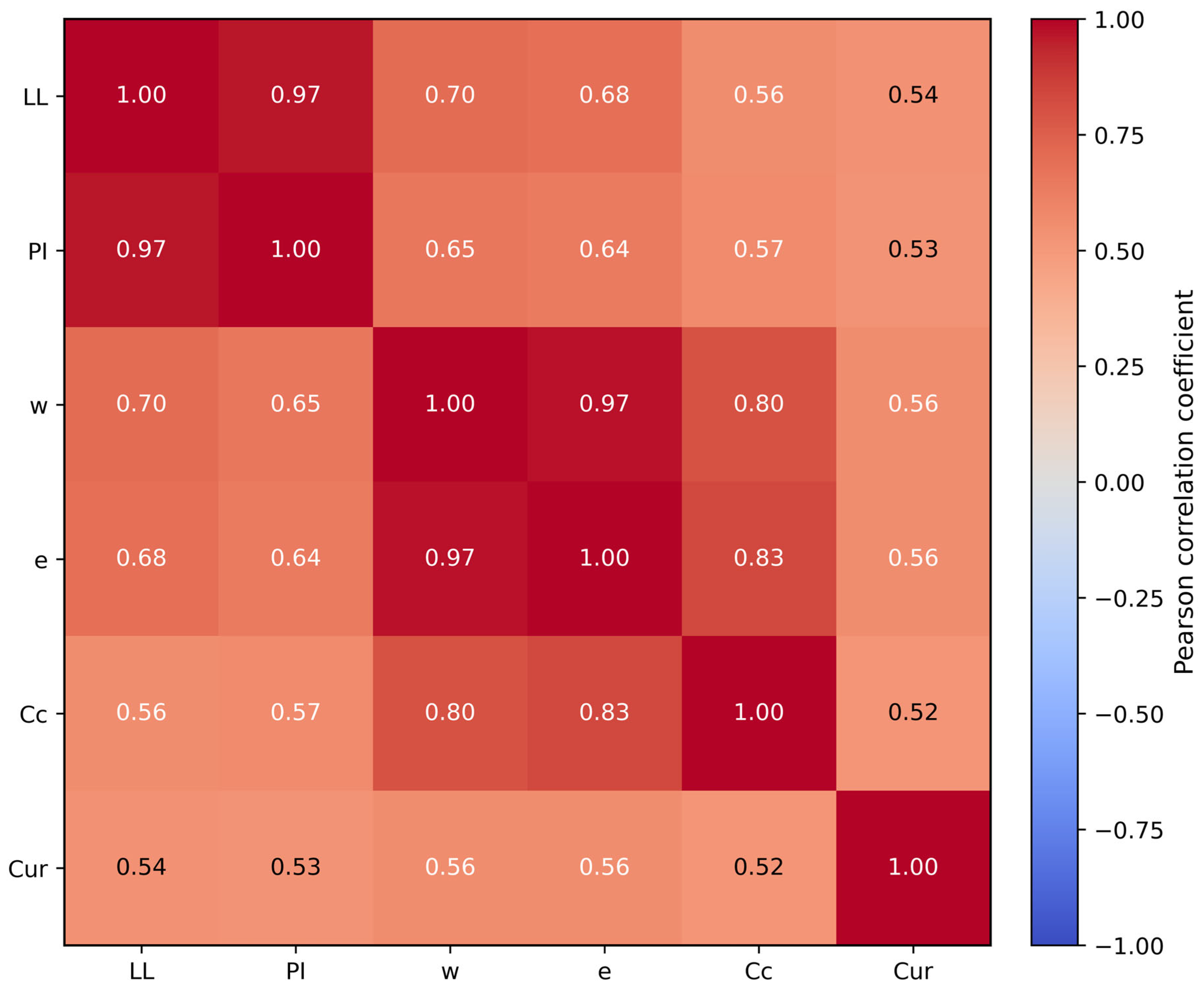
No additional information such as depth, overconsolidation ratio, preconsolidation pressure, mineralogy or in situ test results is used in the primary modelling scenario. This allows the study to quantify what can be achieved using only routinely available index properties, in line with previous correlation and ML-based work on clay compressibility [2,3,4,6,7,8,9,11,12,13,14,15,16,17]. Descriptive statistics and correlations for these variables are summarised in Table 1 and Figure 1.

3.2. Exploratory Analysis and Descriptive Statistics

Descriptive statistics were computed for the cleaned Cc–Cur subset using the mean, standard deviation, minimum, quartiles, median, and maximum values of LL, PI, w, e, Cc, and Cur. These statistics are reported in Table 1. The variables cover a broad range of plasticities, water contents, void ratios, and compressibilities, confirming that the dataset includes low- to very high-plasticity clays, relatively dry to very wet natural states, and dense to very loose initial void structures.

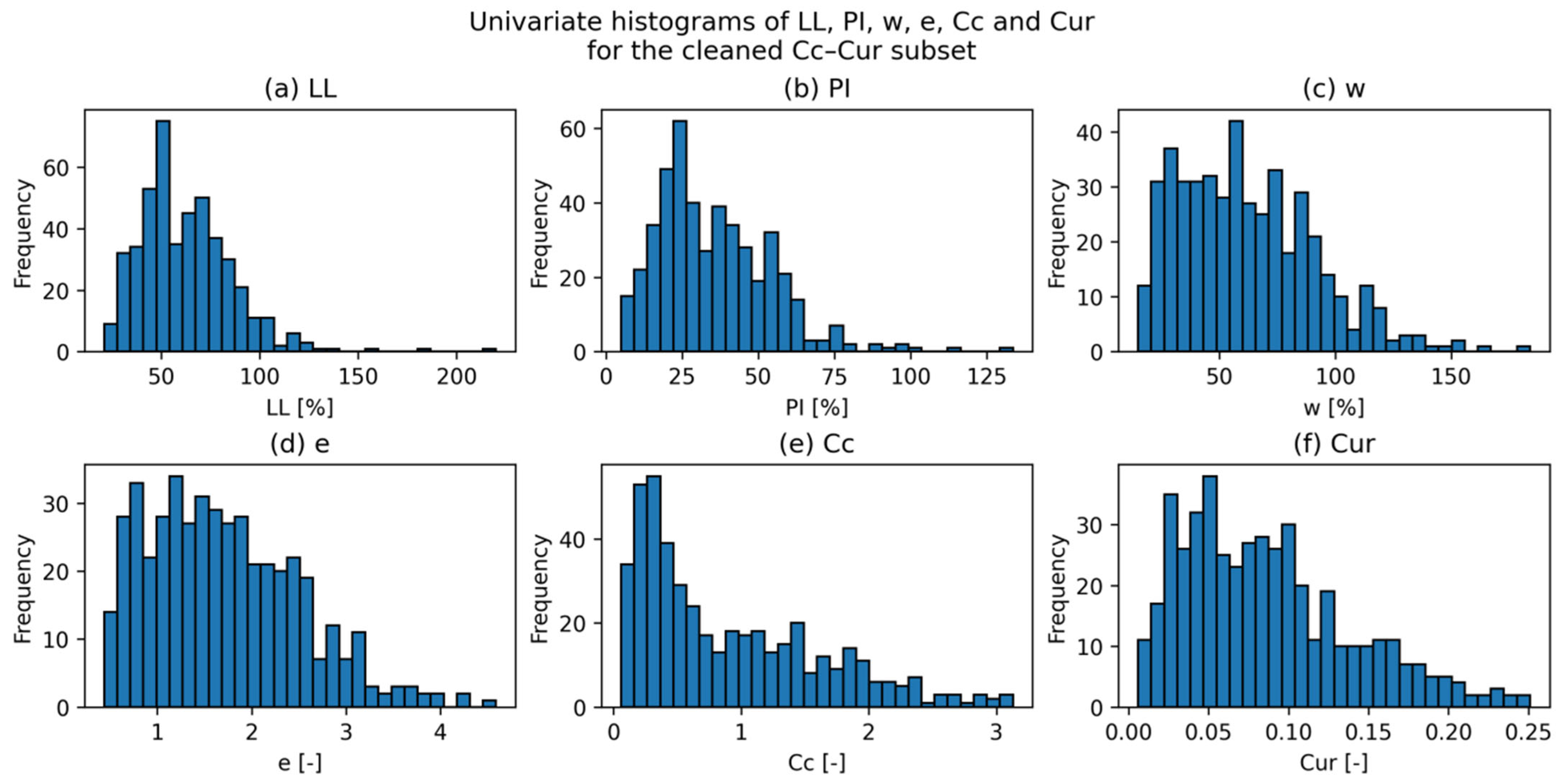
Univariate distributions were then examined using histograms, as shown in Figure 2. Cc and Cur exhibit positively skewed distributions, with long upper tails associated with highly compressible materials [3,18]. The distributions of w and e are also moderately skewed towards higher values, while LL and PI show clustering consistent with standard plasticity groupings. These exploratory checks confirm that the cleaned subset retains sufficient variability in both predictors and target variables for model development and validation.

Correlation Structure and Cc–Cur Relationship

Pearson correlation coefficients among LL, PI, w, e, Cc, and Cur were calculated to assess the linear associations among the input variables and compressibility indices. As shown in Figure 1, LL and PI are strongly correlated, reflecting their common link to clay fraction and mineralogical composition. Cc shows stronger correlations with e and w than with LL and PI, which is consistent with the role of soil state variables in controlling large-strain compressibility [3,4,18]. Cur is positively correlated with the index properties and with Cc, but the correlations are weaker than those observed for Cc.

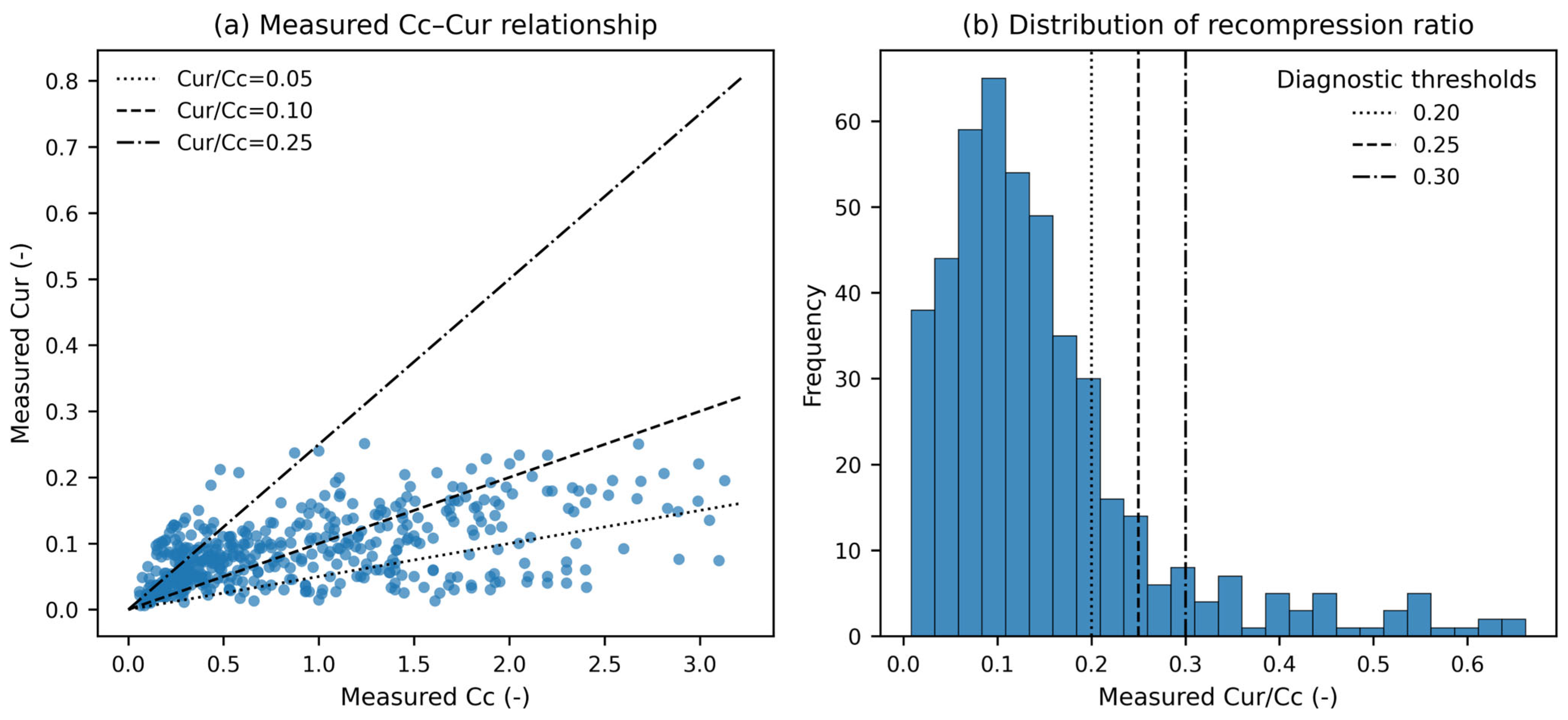
The measured Cc–Cur relationship is shown in Figure 3. Although the two indices follow an overall increasing trend, the scatter is substantial. The distribution of the Cur/Cc ratio further indicates that Cur cannot be represented reliably by a single fixed fraction of Cc across all natural clay samples. This supports the need for paired-output models and physical-consistency checks in addition to conventional error metrics.

3.3. Machine Learning Models and Training Protocol

3.3.1. Problem Definition and Predictors

This study addresses an index-only prediction scenario, in which the compressibility indices Cc and Cur are inferred from four routinely measured properties: LL, PI, w, and e. The objective is to benchmark the achievable performance across model families and to evaluate whether joint modelling improves the physical coherence of the predicted (Cc, Cur) pairs required in consolidation-based settlement calculations.

3.3.2. Algorithm Selection and Justification

Three model families were benchmarked to cover commonly used computational approaches for tabular geotechnical datasets: (i) Random Forest (RF) as a robust nonparametric baseline; (ii) Extreme Gradient Boosting (XGB) as a regularised boosted-tree method that often achieves strong accuracy on structured data; and (iii) fully connected deep neural networks (DNN) as flexible function approximators. Single-output models were trained separately for Cc and Cur. For joint prediction, a true multi-output RF (MO_RF) was used by fitting a single forest to the vector target (Cc, Cur). For boosted trees, a practical paired workflow (MO_XGB) was implemented using a multi-output wrapper that fits one boosted model per target under identical splits and tuning budgets; this is reported to facilitate coherent paired predictions but does not constitute a shared-representation multi-task learner.

3.3.3. Preprocessing

Tree ensembles were trained directly on the raw predictors (LL, PI, w, e). For DNN models, inputs were standardised to zero mean and unit variance using statistics computed on the training partition, only to avoid information leakage. Networks used MSE loss and the Adam optimiser [32,33]; early stopping monitored validation loss on an internal split of the training data.

3.3.4. Cross-Validation Design

The cleaned dataset was randomly split into a training set (80%) and an independent test set (20%) using a fixed seed (random_state = 42). A fixed random seed was used to ensure reproducibility of the train–test split, cross-validation folds, and model comparisons. The value of 42 has no specific statistical meaning and was used only as a reproducibility control. To assess the sensitivity of the reported results to seed selection, additional runs were performed using multiple random seeds. The results, summarised in

Table A2. Baseline equations: 10-fold cross-validation performance for Cc metrics.

Baseline	Cc R2 (Mean ± Std)	Cc RMSE (Mean ± Std)	Cc MAE (Mean ± Std)
Terzaghi–Peck LL + α_train·Ĉc	−0.120 ± 0.045	0.752 ± 0.074	0.514 ± 0.038
Skempton LL + α_train·Ĉc	−0.360 ± 0.045	0.829 ± 0.074	0.574 ± 0.038
Azzouz (e + LL) + α_train·Ĉc	0.331 ± 0.088	0.581 ± 0.077	0.378 ± 0.042
Azzouz (w + LL) + α_train·Ĉc	0.296 ± 0.074	0.597 ± 0.076	0.384 ± 0.043
Reg (e + LL) + α_train·Ĉc	0.366 ± 0.091	0.566 ± 0.077	0.368 ± 0.042
Reg (e + LL) + 0.10·Ĉc	0.366 ± 0.091	0.566 ± 0.077	0.368 ± 0.042
Reg (e + LL) + 0.20·Ĉc	0.366 ± 0.091	0.566 ± 0.077	0.368 ± 0.042
OLS (LL, PI, e, w)	0.713 ± 0.077	0.376 ± 0.042	0.279 ± 0.022
Ridge (λ = 1) (LL, PI, e, w)	0.714 ± 0.077	0.376 ± 0.043	0.279 ± 0.022

, show that the overall model ranking and main conclusions remained generally stable. As expected, the variability was larger for Cur than for Cc, reflecting the weaker constraint of recompression behaviour of the available index properties.

To ensure direct comparability, all random-split model comparisons were evaluated using the same cleaned 459-record dataset, the same 80/20 train–test partition, and the same held-out test set. The term “raw MO-RF” refers only to the multi-output Random Forest trained with the original four predictors LL, PI, e, and w.

3.4. Hyperparameter Tuning

A bounded hyperparameter search space was defined for each model family based on prior studies and preliminary trials. For RF and XGB, random search over discrete grids was used to explore a range of model complexities (e.g., number of trees/estimators, maximum depth, minimum samples per leaf, subsampling and regularisation). For DNNs, a small grid over the architecture and optimisation settings (number of hidden layers, units per layer, learning rate and batch size) was explored with early stopping to control overfitting. The search spaces are listed in

Table 2. Hyperparameter search space for RF, XGB and DNN models.

Model Family	Hyperparameter	Symbol	Search Range/Options	Type
RF/MO_RF	Number of trees	n_estim	100, 200, 300, 400, 500	Discrete
	Maximum tree depth	max_depth	None, 4, 8, 12, 16	Discrete
	Min. samples to split	min_samples_split	2, 4, 6	Discrete
	Min. samples per leaf	min_samples_leaf	1, 2, 4	Discrete
	Max. features per split	max_features	“sqrt”, “log2”, 0.7, 0.9	Categorical
XGB/MO_XGB	Number of trees	n_estim	200, 400, 600, 800	Discrete
	Learning rate	η	0.01, 0.03, 0.05, 0.10, 0.15	Discrete
	Maximum tree depth	max_depth	3, 4, 5, 6, 8	Discrete
	Minimum child weight	min_child_weight	1, 3, 5, 10	Discrete
	Subsample ratio	subsample	0.6, 0.8, 1.0	Discrete
	Column subsample ratio	colsample_bytree	0.6, 0.8, 1.0	Discrete
	L2 regularisation	reg_lambda	0, 1, 5, 10	Discrete
DNN/DNN_MO	Hidden layers	–	1, 2, 3 fully connected layers	Discrete
	Neurons per hidden layer	–	32, 64, 96, 128	Discrete
	Activation function	–	ReLU	Fixed
	Learning rate (Adam)	α	1 × 10−4, 3 × 10−4, 1 × 10−3, 3 × 10−3	Discrete
	Batch size	–	16, 32, 64	Discrete
	Early stopping patience	–	20, 30, 50 epochs	Discrete
	Dropout rate	–	0.0, 0.1, 0.2, 0.3	Discrete

.

Final hyperparameters were selected as the configurations yielding the lowest mean cross-validated RMSE (single-output) or the lowest mean average RMSE across outputs (multi-output), subject to stable R² and the absence of pathological behaviour (e.g., extreme overfitting). The tuned values used in the subsequent analyses are reported in

Table 3. Final tuned hyperparameters for RF, XGB and DNN models used in this study.

Model	Hyperparameter/Setting	Target(s)
		Cc	Cur	Cc, Cur
RF	Number of trees (n_estim)	300	300	300
	Maximum tree depth (max_depth)	None	None	None
	Min. samples to split (min_samples_split)	2	2	2
	Min. samples per leaf (min_samples_leaf)	1	1	1
XGB	Number of trees (n_estim)	400	400	400
	Maximum tree depth (max_depth)	4	4	4
	Minimum child weight (min_child_weight)	1	1	1
	Subsample ratio (subsample)	0.8	0.8	0.8
	Column subsample (colsample_bytree)	0.8	0.8	0.8
	Learning rate (XGB)	0.05	0.05	0.05
DNN	DNN architecture (hidden layers × units)	2 hidden layers × 64 neurons	2 hidden layers × 64 neurons	2 hidden layers × 64 neurons
	Dropout rate	0.0	0.0	0.0
	Learning rate (Adam)	0.001	0.001	0.001
	Batch size	32	32	32

.

3.5. Evaluation Metrics

Predictive performance was quantified for each target using the coefficient of determination (R²), root mean square error (RMSE), and mean absolute error (MAE). Metrics were computed on cross-validation folds and on the held-out test set. For multi-output models, metrics are reported separately for Cc and Cur; during tuning, an aggregate criterion based on the average RMSE across both outputs was used.

3.6. Bootstrap-Based Uncertainty Analysis

To quantify model-related predictive uncertainty, a bootstrap resampling strategy was adopted. For each model family and target configuration, 300 bootstrap samples were generated from the training set with replacement. Models were retrained on each bootstrap sample and evaluated on the fixed held-out test set. The 2.5th and 97.5th percentiles of the bootstrap predictions were used to construct nominal 95% prediction intervals. Prediction interval coverage probability (PICP) and mean prediction interval width (MPIW) were then computed to assess empirical coverage and interval sharpness. These intervals are interpreted as bootstrap-based uncertainty indicators rather than fully calibrated design bounds.

3.7. Model Interpretability and Physical Consistency Checks

Model behaviour was analysed using SHAP for the ensemble models, with emphasis on global feature importance and feature-dependence patterns. Because Cc and Cur are used jointly in one-dimensional consolidation and settlement calculations, the physical plausibility of each predicted pair was also evaluated. Specifically, the predicted values, denoted as Ĉc and Ĉur, were assessed using three complementary diagnostics: (i) the percentage of predictions violating the mechanical admissibility condition Ĉur < Ĉc, reported as cases where Ĉur ≥ Ĉc; (ii) the distribution of the predicted recompression-to-compression ratio, Ĉur/Ĉc, compared with the measured Cur/Cc ratio; and (iii) the geometry of the predicted cloud in the Cc–Cur plane. These diagnostics complement the marginal error metrics and indicate whether the models produce paired predictions that are not only numerically accurate but also physically admissible for consolidation-based settlement assessment.

3.8. Reproducibility and Transparency

All analyses were implemented in Python (version 3.12.12) using standard open-source libraries (pandas version 2.2.3 and NumPy version 2.1.3 for data handling; scikit-learn version 1.6.1 for model training and validation; XGBoost version 2.1.4 for gradient-boosted trees; TensorFlow version 2.18.0 with Keras version 3.8.0 for neural networks; SHAP version 0.46.0 for post hoc explanations). Random seeds were fixed (random_state = 42) for data splitting and model training to ensure repeatability. The curated dataset, full hyperparameter ranges, and final tuned configurations are reported to support transparent reproduction of the modelling workflow.

3.9. Physically Constrained Target Transformation and Geotechnical Feature Enrichment

To further examine whether simple geotechnical constraints can improve the reliability of paired compressibility predictions, a physics-guided modelling strategy was added to the baseline machine learning workflow. The motivation for this additional analysis is that the compression index and recompression index are not independent quantities in a one-dimensional consolidation analysis. For natural clays, the recompression index is expected to be positive and smaller than the compression index, i.e.,:

Cc > 0, Cur > 0, Cur < Cc

(1)

The baseline single-output and multi-output models predicted Cc and Cur directly.

The recompression ratio was defined as:

r = Cur/Cc

(2)

where Cur is the recompression index and Cc is the compression index. Since Cur is expected to be positive and smaller than Cc for natural clays, the physically admissible range is:

0 < r < 1

(3)

In practical geotechnical correlations, the recompression-to-compression ratio Cur/Cc is often approximately in the range of 0.05–0.20, equivalent to the inverse ratio Cc/Cur of about 5–20. However, this study did not impose this narrower empirical range as a hard constraint. Instead, only the broader mechanical admissibility condition 0 < r < 1 was enforced.

The bounded ratio was modelled using the logit transformation:

y₂ = log[r/(1 − r)]

(4)

After prediction, the inverse transformation was applied as:

r̂ = 1/[1 + exp(−ŷ₂)]

(5)

and the recompression index was reconstructed as:

Ĉur = r̂ × Ĉc

(6)

This formulation ensures that the predicted recompression index remains positive and smaller than the predicted compression index.

This approach is referred to here as a physically constrained target transformation, rather than a full physics-informed neural network, because it does not embed the governing differential equation of consolidation. Instead, it incorporates basic geotechnical admissibility conditions into the structure of the prediction task.

In addition to the original four predictors LL, PI, e, and w, a second feature set was constructed using simple geotechnical state and plasticity descriptors. These derived variables were introduced to provide the models with additional physically meaningful combinations of routine index properties:

PL = LL − PI

(7)

LI = (w − PL)/PI

(8)

W/LL, w/e, PI/LL

(9)

where PL is the plastic limit and LI is the liquidity index. These variables were selected because they provide indirect information about the position of the natural water content relative to the Atterberg limits, the water content relative to the void state, and the relative contribution of plasticity to the liquid limit.

It should be noted that this transformation does not impose a fixed Cur/Cc ratio. The ratio r is still learned from the data as a continuous target, while the transformation only restricts predictions to the mechanically admissible range 0 < Cur/Cc < 1. Nevertheless, this constraint may reduce flexibility for samples with an unusual compression–recompression behaviour, particularly if their Cur/Cc ratios lie near the tails of the observed distribution.

The enriched feature set was therefore:

X = {LL, PI, e, w, PL, LI, w/LL, w/e, PI/LL}

(10)

Three modelling configurations were compared:

Raw multi-output RF, using only LL, PI, e, and w, with direct prediction of Cc and Cur;

Geotechnically enriched RF, using the expanded feature set but still predicting Cc and Cur directly;

Physics-guided ratio models, using the expanded feature set and predicting log(Cc) and the transformed ratio Cur/Cc.

Random Forest and Gradient Boosting models were used for the physics-guided ratio formulation. The same train–test split and evaluation metrics used in the main modelling workflow were retained to ensure comparability with the baseline models. Model performance was assessed using R², RMSE and MAE for both Cc and Cur. In addition, paired-output physical consistency was evaluated using the violation rate:

Ĉur ≥ Ĉc

(11)

and the near-violation rate:

Ĉur/Ĉc ≥ 0.25

(12)

The Cur/Cc ≥ 0.25 criterion was used as a high-ratio diagnostic rather than a strict theoretical failure limit. It flags predictions where the recompression index becomes unusually large relative to the compression index. To avoid dependence on a single threshold, additional sensitivity checks were performed using Cur/Cc ≥ 0.20, 0.25 and 0.30.

This formulation should be interpreted as a physically constrained target transformation rather than a full physics-informed or PINN-type model. It does not solve or embed the governing consolidation equations. Instead, it incorporates the basic mechanical admissibility condition Cur < Cc into the prediction structure.

Practical Four-Variable Empirical Formulation

To improve practical usability for engineering applications, a compact four-variable empirical formulation was also derived using only the original routine index properties LL, PI, e, and w. The aim of this formulation was not to replace the machine learning models, but to provide a transparent calculation tool for preliminary site assessment when only limited index data are available. A power-law form was selected because it is simple to apply and gives positive predictions within the calibration range of the database.

The empirical equations are expressed as:

Cc = 0.6508, LL^−0.9543 PI^0.7976 e^1.3588 w^0.1383

(13)

Cur = 0.001322, LL^0.4525 PI^0.1604 e^−0.0244 w^0.3979

(14)

where LL, PI, and w are expressed in percents, and e is dimensionless. These equations were calibrated using the cleaned 459-record Cc–Cur subset and should be used only within the calibration range of the database: LL = 21–220%, PI = 5–133.6%, e = 0.437–4.587, and w = 15–184%.

3.10. Site-/Location-Aware Validation Protocol

In addition to the random train–test and cross-validation protocol, a site-/location-aware validation was performed to evaluate the robustness of the models under a more conservative separation of geotechnical sources. This additional analysis was motivated by the possibility that records originating from the same project, site, or nearby clay deposit may share geological and procedural characteristics. Under a purely random split, such related records may be distributed across both the training and testing subsets, potentially producing optimistic estimates of generalisation performance.

Because the cleaned modelling table retained only the numerical variables used for prediction, each of the 459 cleaned records was first matched back to the original CLAY/Cc/6/6203 database using the six numerical fields LL, PI, w, e, Cc, and Cur. All 459 records were successfully matched. The recovered metadata fields included Site, Country, and City/Location. A conservative grouping variable was then defined using the combination of Country and City/Location. This grouping was preferred over the Site field alone because several nearby or related site identifiers may occur within the same geological area; grouping by Country–Location, therefore, reduces potential spatial or project-level leakage between the training and testing folds.

The leave-one-location-out (LOLO) procedure was implemented by holding out all records from one Country–Location group as the test subset while training the model on all remaining groups. This process was repeated until each group had been used once as the external validation group. The resulting out-of-group predictions were then pooled and evaluated using R², RMSE, and MAE for Cc and Cur. Pairwise physical consistency was also assessed using the violation rate, defined as the percentage of predictions for which Ĉur ≥ Ĉc, and a near-violation diagnostic, defined as Ĉur/Ĉc ≥ 0.25 (See

Table 4. LOLO validation and sensitivity to small Country–Location groups.

Model	LOLO Scenario	n Samples	n Groups	Cc R2	Cc MAE	Cur R2	Cur MAE	Cur/Cc ≥ 0.25 (%)
RF enriched	all 81 groups	459	81	0.697	0.274	0.187	0.037	9.150
RF enriched	test groups with n ≥ 2	437	59	0.702	0.275	0.175	0.037	8.009
RF enriched	test groups with n ≥ 4	376	34	0.721	0.266	0.130	0.038	7.713
GCTT RF	all 81 groups	459	81	0.717	0.253	0.142	0.037	10.240
GCTT RF	test groups with n ≥ 2	437	59	0.725	0.254	0.136	0.038	8.696
GCTT RF	test groups with n ≥ 4	376	34	0.747	0.245	0.100	0.039	8.511
RF raw	all 81 groups	459	81	0.669	0.285	0.179	0.037	8.279
RF raw	test groups with n ≥ 2	437	59	0.673	0.286	0.166	0.037	7.094
RF raw	test groups with n ≥ 4	376	34	0.703	0.273	0.123	0.038	7.181

).

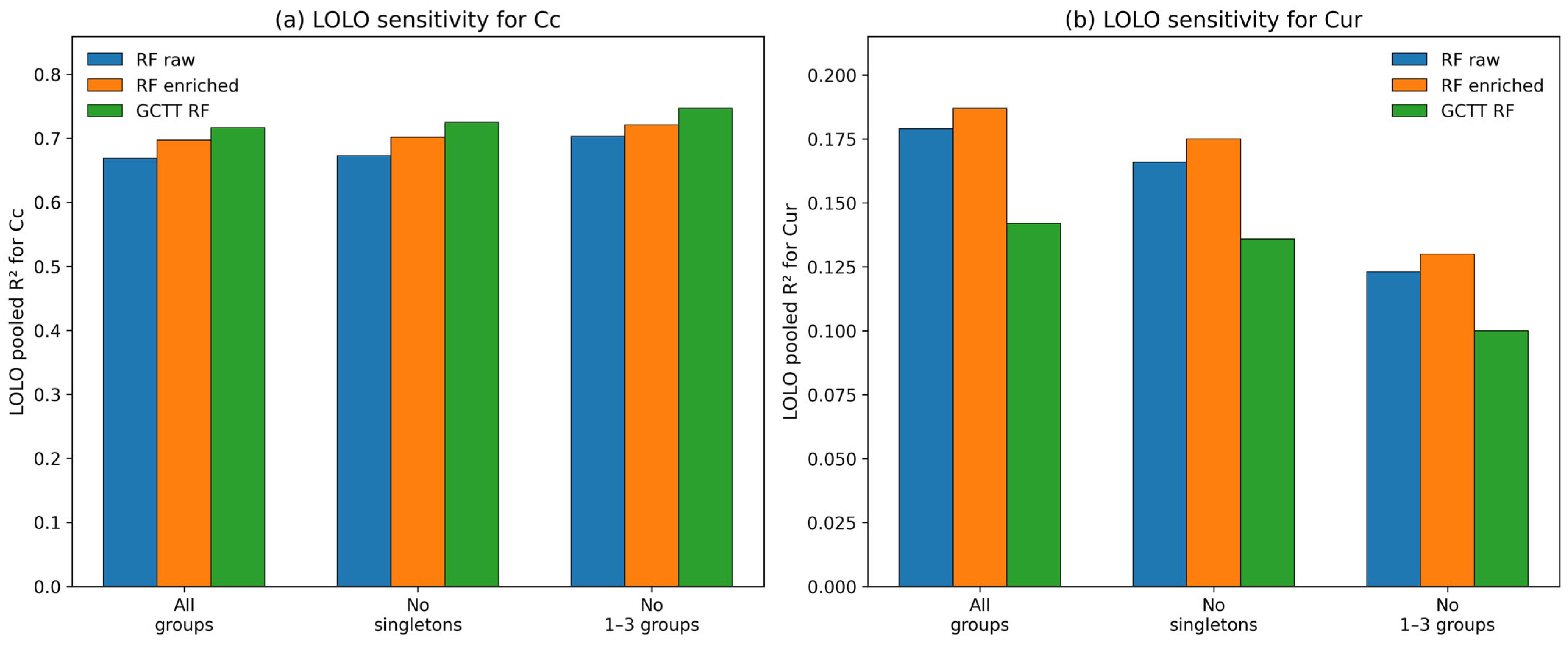
The sensitivity analysis indicates that the small Country–Location groups do not control the main conclusions of the LOLO validation. For Cc, removing singleton groups and groups with one to three records slightly increased the pooled R², indicating that the predictive trend for Cc is reasonably stable under different group-size filters. For Cur, however, the pooled R² decreased after excluding the smallest groups, whereas the MAE remained almost unchanged. This suggests that the low LOLO performance for Cur is not simply an artefact of singleton groups but reflects the limited transferability of recompression behaviour when stress-history, fabric, bonding and geological descriptors are unavailable (See Figure 4).

4. Results

4.1. Descriptive Statistics and Correlation Structure

The cleaned dataset consists of 459 natural clay samples with complete measurements of LL, PI, w, e, Cc, and Cur. As summarised in Table 1 and Figure 1, Figure 2 and Figure 3, the dataset spans a wide range of index properties and compressibility values. Cc varies over more than an order of magnitude, while Cur is generally much smaller but still shows considerable variability.

The exploratory results show that Cc is more strongly associated with e and w than with LL and PI, confirming that compression behaviour is mainly governed by the current soil state rather than plasticity alone. In contrast, Cur shows weaker correlations with all four index properties and with Cc. The Cc–Cur scatter plot shows a positive but dispersed relationship, and the Cur/Cc ratio has a median of about 0.10 with a wide interquartile range. This indicates that the two indices are physically coupled but not deterministically linked by a constant ratio.

These findings motivate the use of joint prediction models that can estimate Cc and Cur simultaneously while also checking whether the predicted pairs remain mechanically admissible, particularly with respect to the condition Cur < Cc.

4.2. Single-Output Ensemble Model Performance

Single-output RF and XGB models were first trained separately for each target using LL, PI, e, and w as inputs. The 10-fold cross-validation and test-set metrics are reported in

Table 5. Cross-validation and test-set performance of single-output RF, XGB and DNN models for Cc and Cur (R², RMSE, MAE).

Target	Model	CV R2 (Mean ± Std)	CV RMSE (Mean ± Std)	CV MAE (Mean ± Std)	Test R2	Test RMSE	Test MAE
Cc	RF	0.732 ± 0.066	0.354 ± 0.069	0.244 ± 0.042	0.611	0.471	0.308
	XGB	0.722 ± 0.110	0.357 ± 0.095	0.246 ± 0.061	0.637	0.455	0.311
	DNN	0.783 ± 0.078	0.315 ± 0.065	0.219 ± 0.037	0.697	0.416	0.283
Cur	RF	0.321 ± 0.125	0.042 ± 0.006	0.031 ± 0.004	0.286	0.043	0.034
	XGB	0.253 ± 0.133	0.044 ± 0.006	0.033 ± 0.004	0.290	0.043	0.034
	DNN	0.403 ± 0.154	0.039 ± 0.006	0.030 ± 0.005	0.196	0.046	0.034

.

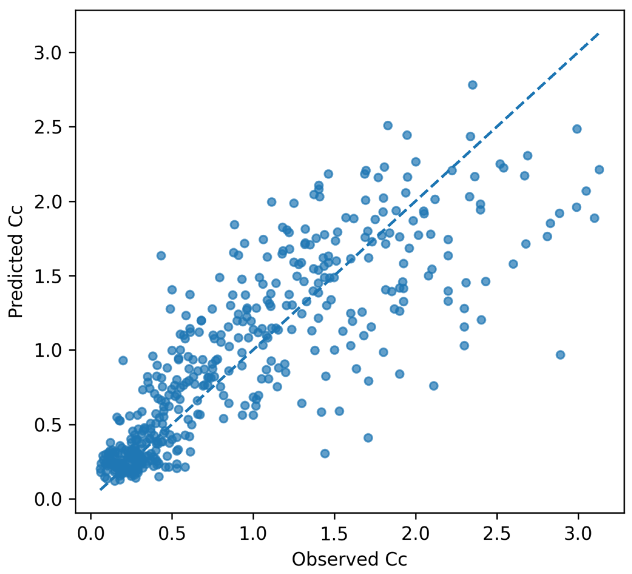
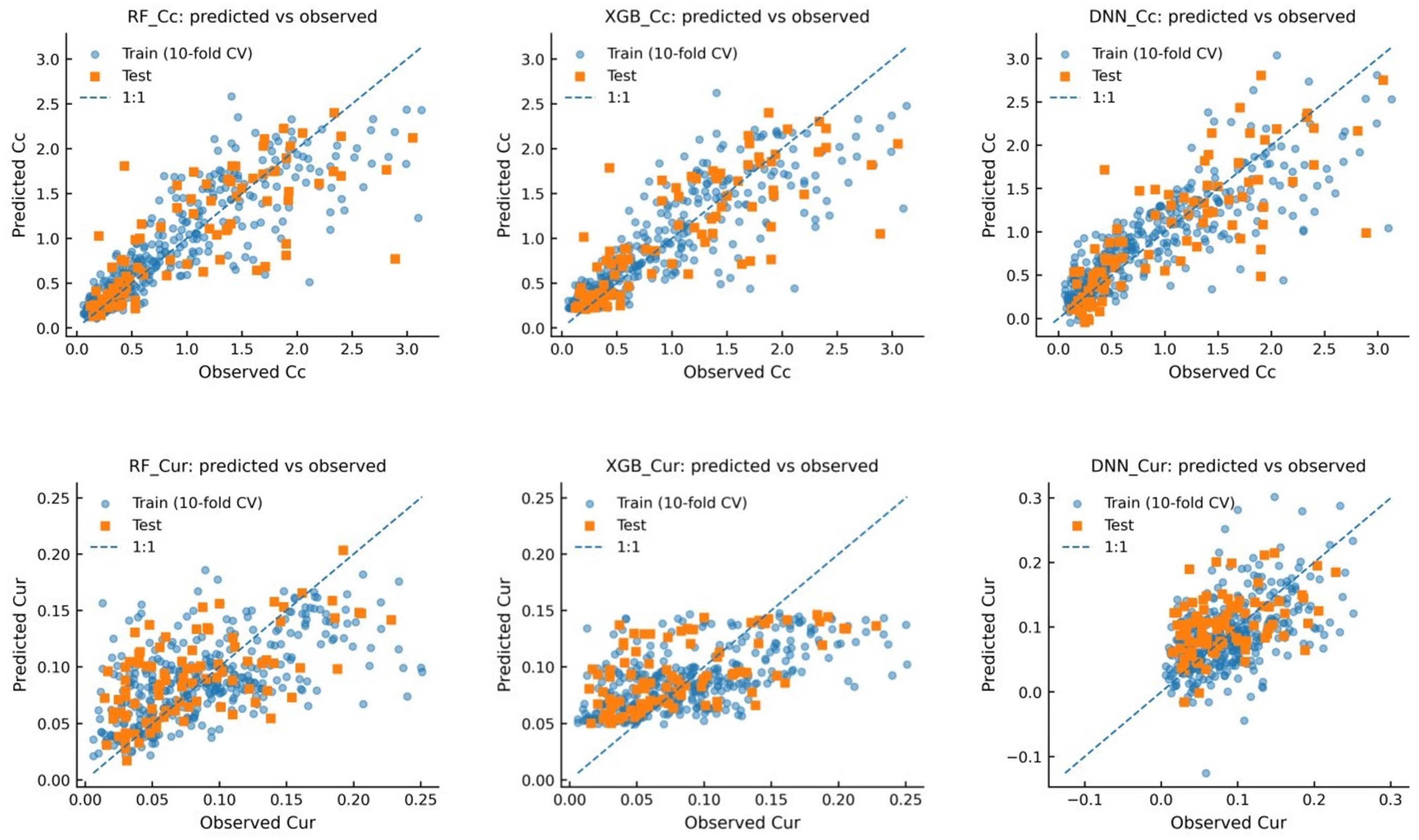
For Cc, RF_Cc attains a cross-validated R² of 0.732 ± 0.066 with RMSE = 0.354 ± 0.069 and MAE = 0.244 ± 0.042. On the independent test set, the model achieves R² = 0.611, RMSE = 0.471 and MAE = 0.308. XGB_Cc exhibits very similar behaviour, with a cross-validated R² = 0.722 ± 0.110 (RMSE = 0.357 ± 0.095, MAE = 0.246 ± 0.061) and slightly higher test-set skill (R² = 0.637, RMSE = 0.455, MAE = 0.311). The predicted–observed plots in Figure 5 show dense point clouds around the 1:1 line, although the models tend to under-predict the largest Cc values. The error metrics in Table 5 indicate acceptable Cc performance but substantially weaker Cur prediction.

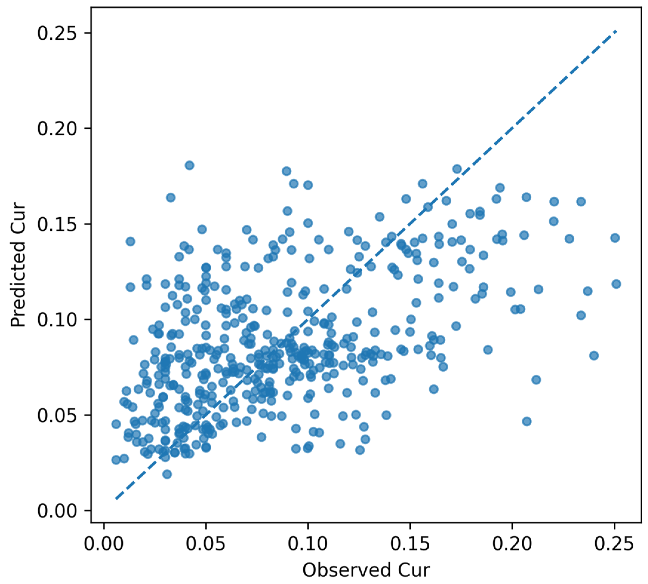
For Cur, the attainable accuracy is noticeably lower. RF_Cur yields cross-validated R² = 0.321 ± 0.125 (RMSE = 0.042 ± 0.006, MAE = 0.031 ± 0.004) and test-set R² = 0.286, with RMSE = 0.043 and MAE = 0.034. XGB_Cur performs comparably, with cross-validated R² = 0.253 ± 0.133 (RMSE = 0.044 ± 0.006, MAE = 0.033 ± 0.004) and test-set R² = 0.290 (RMSE = 0.043, MAE = 0.034). The corresponding predicted–observed and residual plots occupy a narrow numerical range but show relatively larger scatter about the 1:1 line, reflecting that only roughly 30% of the Cur variance is captured by LL, PI, e and w.

Table 6. Quantitative uncertainty diagnostics for single-output models using bootstrap-derived nominal 95% prediction intervals.

Model	Target	R2	RMSE	MAE	PICP	MPIW
RF	Cc	0.611	0.471	0.308	0.533	0.498
	Cur	0.286	0.043	0.034	0.413	0.0528
XGB	Cc	0.637	0.455	0.311	0.554	0.538
	Cur	0.290	0.043	0.034	0.467	0.0607
DNN	Cc	0.697	0.416	0.283	0.620	0.528
	Cur	0.196	0.046	0.034	0.565	0.0738

PICP = Prediction interval coverage probability; MPIW = Mean prediction interval width.

reports the corresponding accuracy metrics together with the prediction interval coverage probability (PICP) and mean prediction interval width (MPIW).

As shown in Table 6, DNN provides the lowest RMSE for Cc, whereas RF and XGB yield comparable performance for Cur. However, the bootstrap-based 95% intervals show limited empirical coverage, with PICP values ranging from 0.533 to 0.620 for Cc and from 0.413 to 0.565 for Cur. This indicates that bootstrap resampling mainly captures model-related uncertainty and does not fully represent the total predictive uncertainty arising from data noise, site heterogeneity and missing descriptors such as stress history and fabric. The relatively low PICP values are particularly important for Cur, confirming that recompression behaviour remains weakly constrained by index properties alone. Therefore, the intervals should be interpreted as comparative uncertainty indicators rather than fully calibrated design bounds.

4.3. Multi-Output Ensembles and Joint Cc–Cur Consistency

Multi-output RF (MO_RF) and XGB (MO_XGB) models were then trained to predict the pair (Cc, Cur) jointly from LL, PI, e, and w. The corresponding metrics are summarised in

Table 7. Cross-validation and test-set performance of multi-output RF, XGB, and DNN models (MO_RF, MO_XGB, DNN_MO) for Cc and Cur.

Target	Model	CV R2 (Mean ± Std)	CV RMSE (Mean ± Std)	CV MAE (Mean ± Std)	Test R2	Test RMSE	Test MAE
Cc	MO_RF	0.736 ± 0.067	0.351 ± 0.070	0.242 ± 0.043	0.612	0.470	0.308
	MO_XGB	0.722 ± 0.110	0.357 ± 0.095	0.246 ± 0.061	0.637	0.455	0.311
	DNN_MO	0.784 ± 0.070	0.315 ± 0.063	0.218 ± 0.034	0.685	0.424	0.288
Cur	MO_RF	0.374 ± 0.123	0.040 ± 0.006	0.030 ± 0.004	0.287	0.043	0.035
	MO_XGB	0.253 ± 0.133	0.044 ± 0.006	0.033 ± 0.004	0.290	0.043	0.034
	DNN_MO	0.296 ± 0.161	0.042 ± 0.004	0.034 ± 0.004	0.189	0.046	0.037

Average RMSE over both targets (CV): 0.196 ± 0.035 (MO_RF), 0.201 ± 0.048 (MO_XGB), 0.179 ± 0.031 (DNN_MO).

.

For Cc, MO_RF delivers cross-validated R² = 0.736 ± 0.067, RMSE = 0.351 ± 0.070, and MAE = 0.242 ± 0.043, with test-set R² = 0.612, RMSE = 0.470, and MAE = 0.308. MO_XGB achieves cross-validated R² = 0.722 ± 0.110, RMSE = 0.357 ± 0.095, and MAE = 0.246 ± 0.061, as well as test-set R² = 0.637, RMSE = 0.455, and MAE = 0.311. These values are essentially indistinguishable from the single-output RF_Cc and XGB_Cc results, indicating that enforcing joint prediction does not compromise Cc accuracy.

For Cur, the benefits of joint modelling are more apparent. MO_RF improves cross-validated performance relative to RF_Cur, attaining R² = 0.374 ± 0.123 with RMSE = 0.040 ± 0.006, and MAE = 0.030 ± 0.004, while maintaining similar test-set metrics (R² = 0.287, RMSE = 0.043, MAE = 0.035). As expected from its formulation, MO_XGB reproduces the XGB_Cur metrics (cross-validated R² = 0.253 ± 0.133, RMSE = 0.044 ± 0.006; test-set R² = 0.290, RMSE = 0.043, MAE = 0.034). The average cross-validated RMSE over both targets is 0.196 ± 0.035 for MO_RF and 0.201 ± 0.048 for MO_XGB, similar to the single-output ensemble averages.

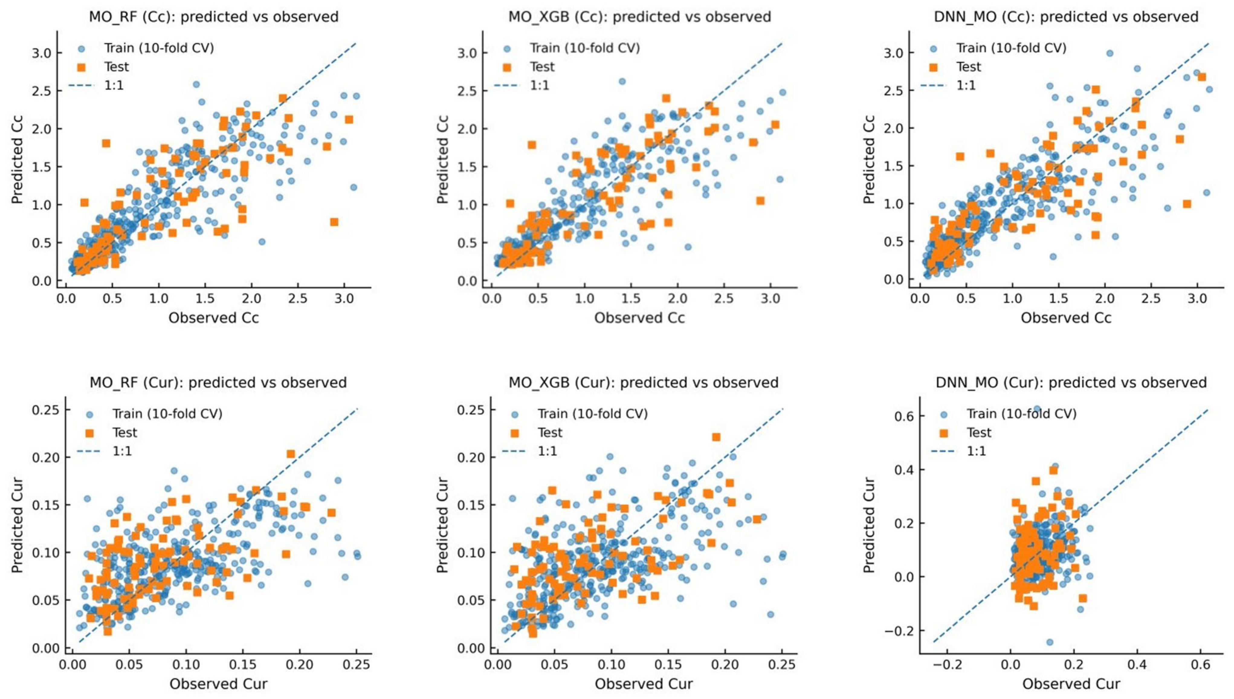
The primary advantage of the multi-output models is the improved physical coherence of their predicted (Cc, Cur) pairs. On the test set, neither MO_RF nor MO_XGB produces any case where Cur exceeds Cc (0 of 92 samples). The observed Cur/Cc ratio has a median of approximately 0.097 and an IQR [0.053, 0.155]. MO_RF predicts a median ratio of approximately 0.097 with an IQR [0.073, 0.150], and MO_XGB predicts a median ratio of approximately 0.099 with an IQR [0.071, 0.144], capturing the central tendency while slightly compressing the upper tail. Joint prediction plots show compact clouds lying below the 1:1 line and mostly within plausible envelopes (for example, Cur ≈ 0.1–0.3 Cc), confirming that the multi-output ensembles generate geotechnically realistic Cc–Cur combinations without sacrificing predictive skill. These features are illustrated in Figure 6, which depicts the predicted–observed relationships for the multi-output ensembles and the DNN_MO benchmark.

To further quantify the reliability of the paired-output predictions, bootstrap-based uncertainty diagnostics were computed for the multi-output RF, XGB and DNN models. In each bootstrap iteration, both target variables, Cc and Cur, were resampled jointly and predicted as a coupled output vector. The 2.5th and 97.5th percentiles of the bootstrap predictions were then used to construct nominal 95% prediction intervals for each target. The resulting accuracy and uncertainty metrics are summarised in

Table 8. Quantitative uncertainty diagnostics for multi-output models using bootstrap-derived nominal 95% prediction intervals.

Model	Target	R2	RMSE	MAE	PICP	MPIW
MO_RF	Cc	0.612	0.470	0.308	0.565	0.499
	Cur	0.287	0.043	0.035	0.370	0.049
MO_XGB	Cc	0.637	0.455	0.311	0.554	0.538
	Cur	0.290	0.043	0.034	0.467	0.061
DNN_MO	Cc	0.685	0.424	0.288	0.543	0.431
	Cur	0.189	0.046	0.037	0.609	0.080

PICP = Prediction interval coverage probability; MPIW = Mean prediction interval width.

.

The results show that the multi-output DNN provides the lowest test-set error for Cc, with R² = 0.685 and RMSE = 0.424, whereas the three multi-output models show comparable but limited performance for Cur. This confirms that Cur remains substantially less identifiable from LL, PI, w, and e than Cc, even under a paired-output learning strategy. The bootstrap-derived prediction intervals provide additional insight into model reliability. For Cc, the PICP values range from 0.543 to 0.565, while for Cur, they range from 0.370 to 0.609. These values are below the nominal 95% level, indicating that bootstrap resampling mainly captures model-related uncertainty and does not fully represent the total predictive uncertainty associated with site heterogeneity, measurement noise, and missing stress-history or fabric descriptors. Therefore, the intervals should be interpreted as comparative uncertainty indicators rather than fully calibrated design bounds.

Importantly, despite the limited marginal coverage, all multi-output models preserve the basic mechanical admissibility condition Cur < Cc on the test set. As shown in

Table 9. Joint physical consistency and paired-output uncertainty diagnostics of multi-output models.

Model	Joint PICP	Violation Rate Cur ≥ Cc	Near Violation Rate Cur/Cc ≥ 0.25	Median Predicted Cur/Cc
MO_RF	0.228	0.000	0.065	0.096
MO_XGB	0.293	0.000	0.098	0.099
DNN_MO	0.380	0.000	0.022	0.095

Joint PICP = the fraction of test samples for which both Cc and Cur are simultaneously covered by their bootstrap-derived intervals; near-violation rate = the fraction of cases with predicted Cur/Cc ≥ 0.25.

, the violation rate is 0.0% for MO_RF, MO_XGB and DNN_MO. Moreover, the predicted median Cur/Cc ratios remain close to the observed median value of 0.097, with predicted medians of 0.096, 0.099 and 0.095 for MO_RF, MO_XGB and DNN_MO, respectively. This confirms that the multi-output framework improves the physical coherence of paired compressibility predictions, even when the marginal prediction intervals are not fully calibrated.

4.4. Deep Neural Network Benchmarks

A multi-output deep neural network (DNN_MO) and two single-output networks (DNN_Cc and DNN_Cur) were considered as flexible, high-capacity benchmarks.

For Cc, DNN_MO attains cross-validated R² = 0.784 ± 0.070, RMSE = 0.315 ± 0.063, and MAE = 0.218 ± 0.034, with test-set R² = 0.685, RMSE = 0.424, and MAE = 0.288. The single-output DNN_Cc shows nearly identical cross-validation performance (R² = 0.783 ± 0.078, RMSE = 0.315 ± 0.065, MAE = 0.219 ± 0.037) and slightly better generalisation, reaching test-set R² = 0.697, RMSE = 0.416, and MAE = 0.283. Thus, DNN_Cc is the numerically best Cc model in this study, improving test-set R² by roughly 0.05–0.08 relative to the tree ensembles.

For Cur, however, the deep networks do not outperform the ensembles. DNN_MO yields cross-validated R² = 0.296 ± 0.161, RMSE = 0.042 ± 0.004, and MAE = 0.034 ± 0.004, but only R² = 0.189 with RMSE = 0.046 and MAE = 0.037 on the test set. DNN_Cur achieves somewhat higher cross-validated skill (R² = 0.403 ± 0.154, RMSE = 0.039 ± 0.006, MAE = 0.030 ± 0.005) but still attains test-set R² = 0.196 with RMSE = 0.046, and MAE = 0.034. Both networks, therefore, underperform the tree-based models for Cur, for which the test-set R² remains near 0.29, and the RMSE is lower.

The larger drop from cross-validation to test performance for DNN_Cur suggests that the network may partially overfit noisy or site-specific patterns in the Cur labels. This is plausible because Cur is small in magnitude and strongly affected by stress history, fabric and sample disturbance, which are not directly represented by LL, PI, w and e. In contrast, the RF and XGB models appear more resistant to this noise because ensemble averaging, subsampling and tree-level regularisation reduce sensitivity to individual noisy observations. Therefore, although DNNs provide a useful high-capacity benchmark, tree-based models offer a more stable and interpretable option for Cur prediction under the index-only input scenario.

Taken together, these benchmarks suggest that deep learning provides a modest upper bound on what can be achieved from index properties alone for Cc but does not overcome the intrinsic difficulty of predicting Cur in the absence of additional information on stress history and fabric. Given their more complex calibration and lack of native interpretability, the deep networks are retained as reference models, while tree ensembles are adopted as the primary tools in the remainder of the paper.

4.5. SHAP-Based Interpretation of Ensemble Models

SHAP analyses were conducted for MO_RF and the XGB models to clarify how LL, PI, e, and w drive the predictions and to assess the physical plausibility of the learned relationships.

4.5.1. Global Feature Importance

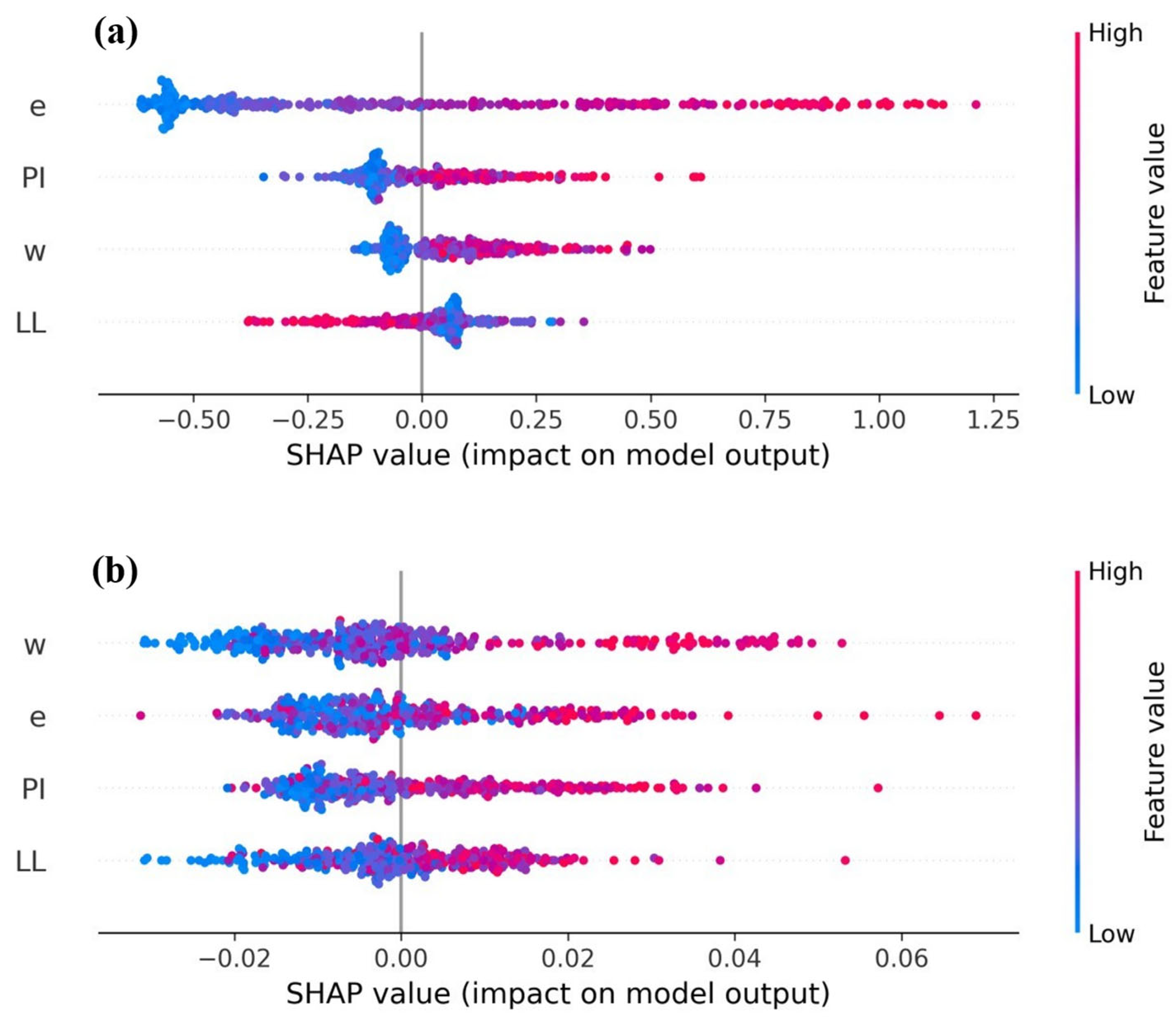
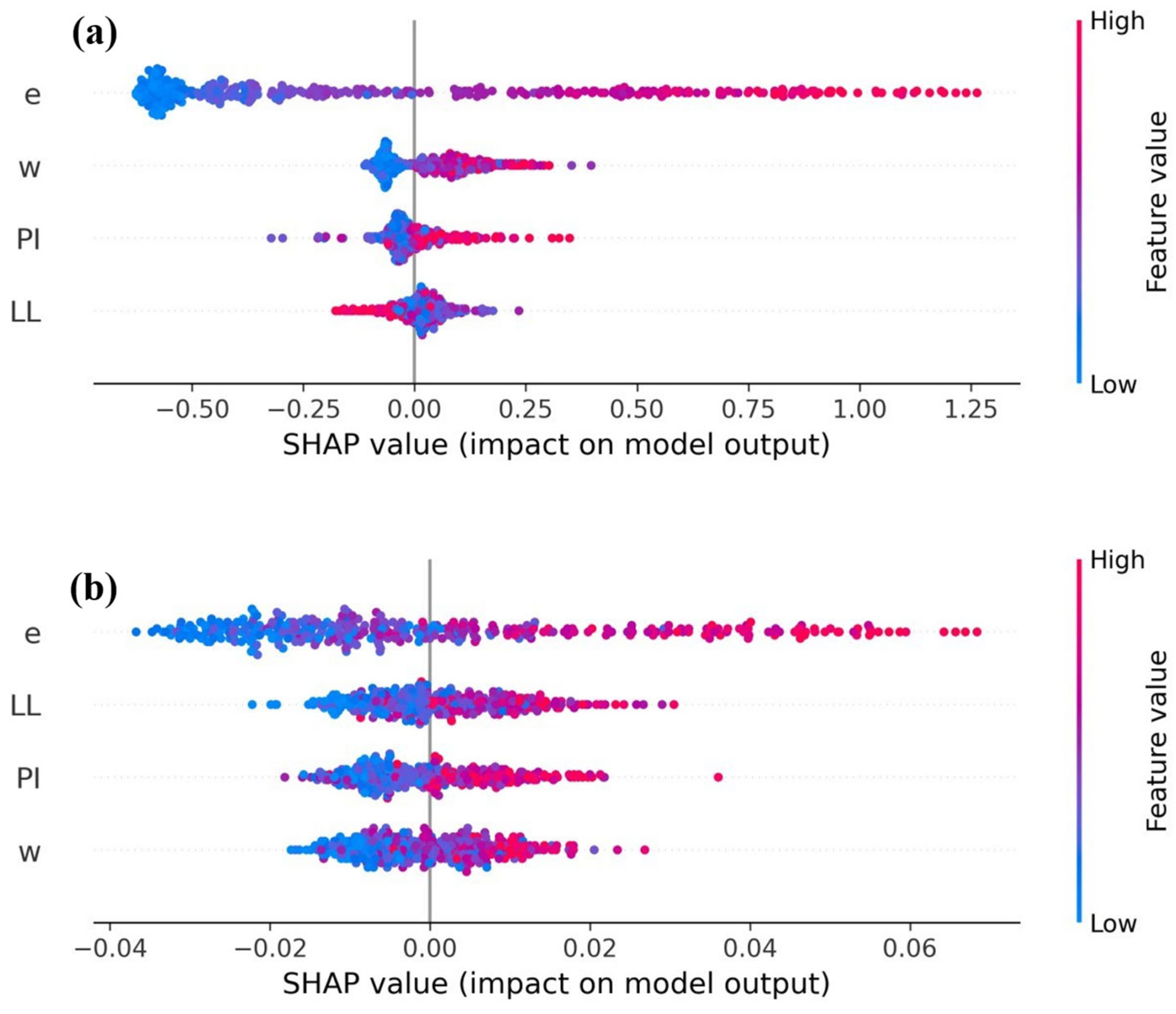
Global SHAP beeswarm plots for the single-output XGB models (See Figure 7 and Figure 8) show a geotechnically consistent ranking for Cc. The initial void ratio (e) is the dominant predictor, followed by natural water content (w) and plasticity index (PI), while liquid limit (LL) has the lowest overall impact. This ordering mirrors the correlation analysis and conventional understanding that loose, wet and highly plastic clays are most compressible.

For Cur, SHAP magnitudes are smaller and more evenly distributed across features in both the single-output XGB models and the multi-output ensembles. No single predictor clearly dominates, and all four index properties exhibit modest and comparable spreads in SHAP values. This diffuse importance pattern is consistent with the lower R² values for Cur and suggests that crucial aspects of stress history and microstructure are only weakly encoded in LL, PI, w, and e.

4.5.2. Non-Linear Effects and Interactions

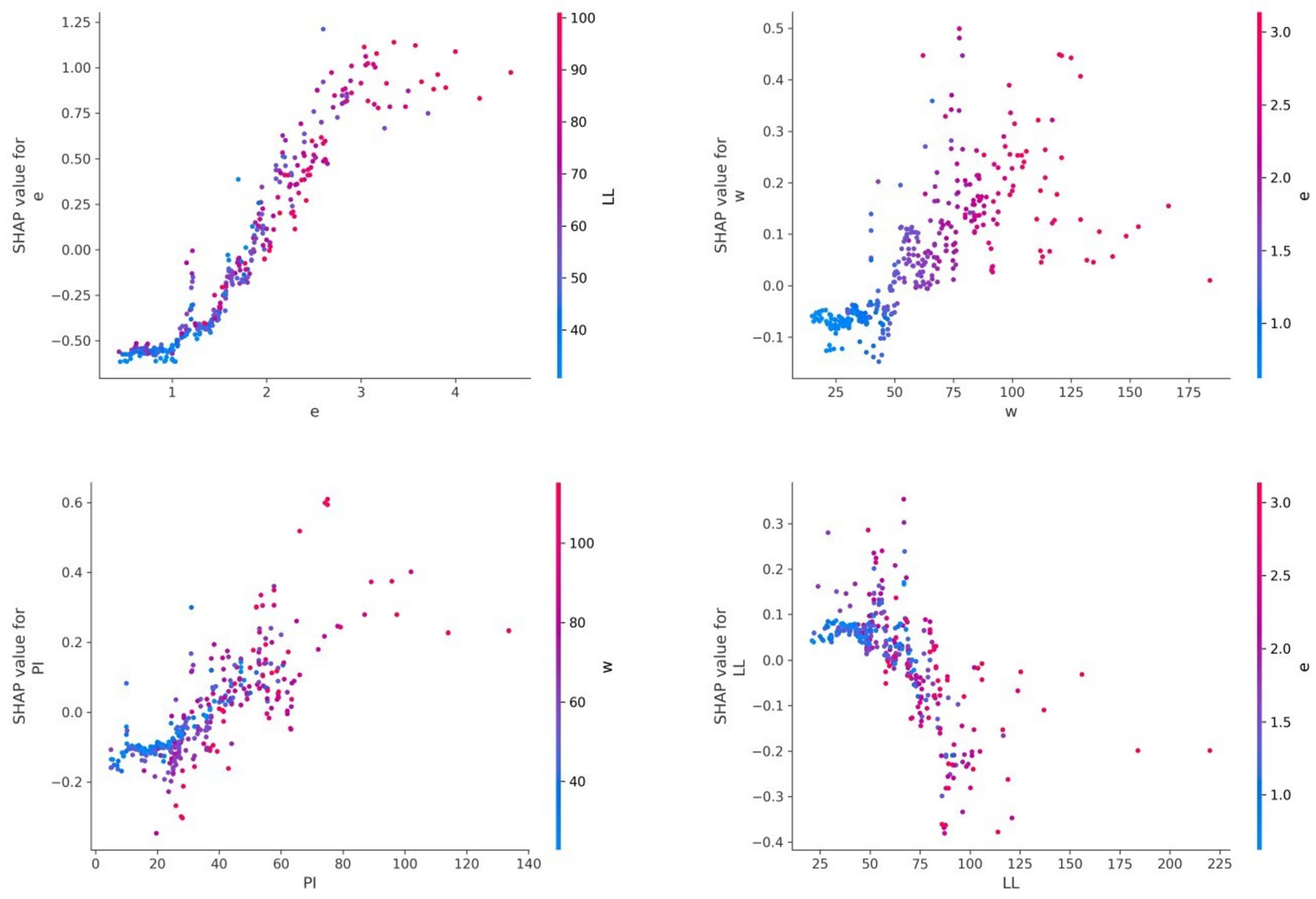
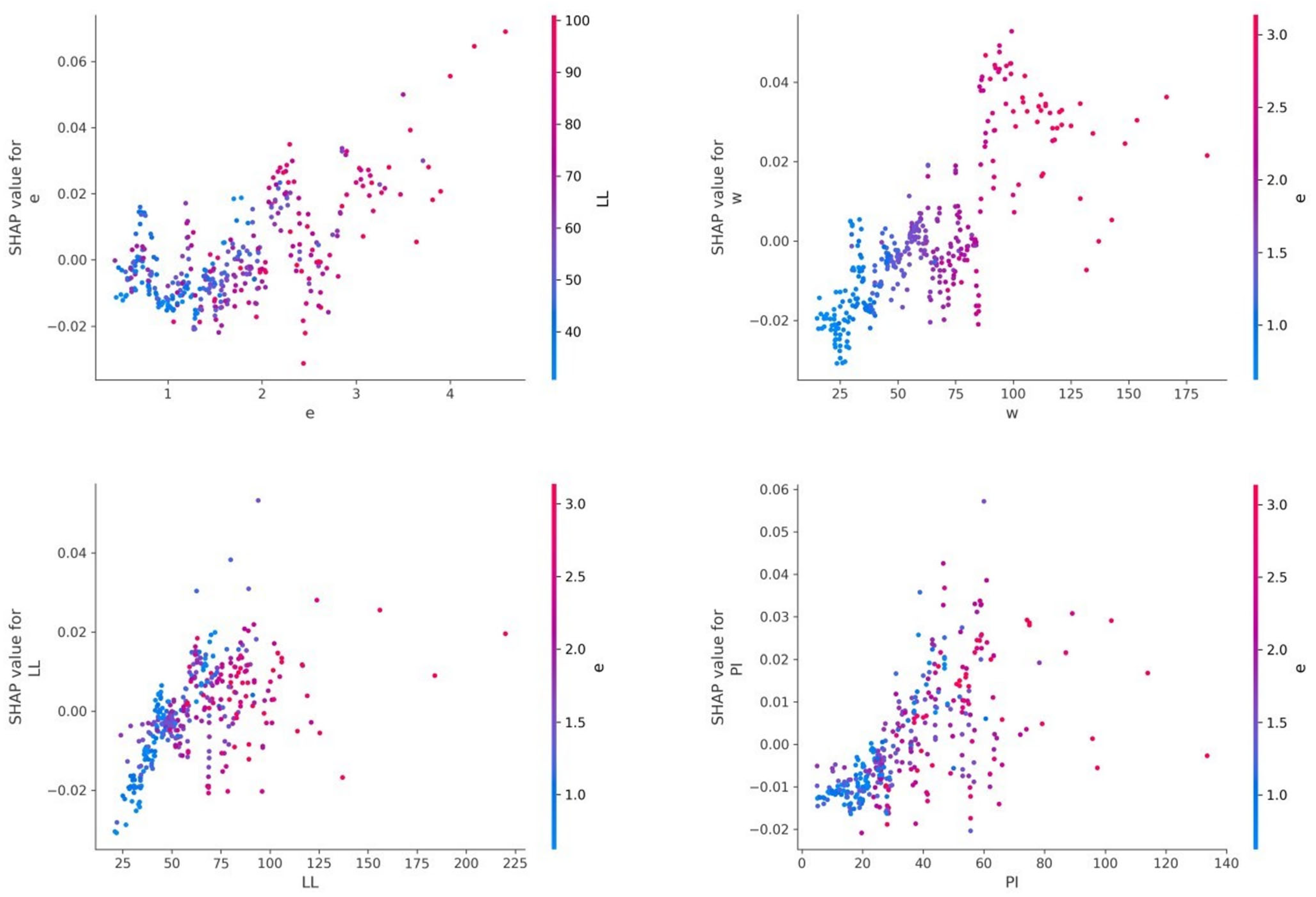
SHAP dependence plots for XGB_Cc (Figure 9) reveal strongly non-linear effects. For e, the SHAP values increase sharply beyond e ≈ 1.0, while w and PI also exhibit curved responses with larger positive contributions at higher water contents and plasticity. Colour-coding the points by LL, PI, or e highlights the interactions: the largest positive contributions occur when high void ratios coincide with high water contents and high plasticity, a signature of very compressible clays.

For Cur (Figure 10), the dependence plots display similar directions of effect but with markedly smaller magnitudes. The SHAP values cluster tightly around zero across the explored ranges of LL, PI, w, and e, again pointing to the influence of unobserved factors such as preconsolidation and bonding.

Overall, the SHAP analysis demonstrates that the ensemble models are not opaque “black boxes”: they recover and quantify known empirical trends in clay compressibility, clarify the non-linear and interactive nature of the relationships, and explain why Cc is substantially more predictable than Cur under the index-only scenario considered in this study.

4.6. Physical Interpretation and Sensitivity of Learned Relationships

The interpretability results are consistent with the geotechnical expectations. Across the ensemble models, SHAP rankings show that the compression index Cc is mainly controlled by the state variables void ratio, e, and natural water content, w, while LL and PI play secondary roles. This confirms that Cc is primarily state-dependent rather than governed by plasticity alone.

For Cur, SHAP magnitudes are smaller and more diffuse, indicating that LL, PI, e, and w provide only limited information for recompression behaviour. This explains why Cur remains more difficult to predict than Cc under the index-only modelling scenario.

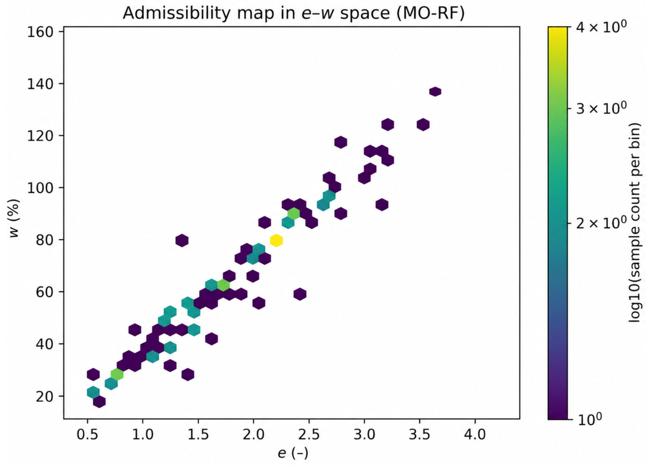
Paired-output admissibility was also assessed for the multi-output RF model in the e–w feature space, as shown in Figure 11. No mechanically inadmissible predictions were observed on the held-out test set, with a violation rate of 0.0% for Ĉur ≥ Ĉc. Near-violations, defined as Ĉur/Ĉc ≥ 0.25, occurred in seven test samples, or 7.6%, and were mainly located in sparsely populated regions of the e–w space. This indicates that the coupled-output predictions remain physically consistent, while high-ratio cases are more likely in regions with limited training data.

4.7. Performance of Physics-Guided and Geotechnically Enriched Models

The physics-guided modelling experiment examined whether derived geotechnical descriptors and a constrained Cur/Cc ratio formulation could improve the paired prediction of Cc and Cur. Four configurations were compared: the raw multi-output RF model, the geotechnically enriched RF model, and two physics-guided ratio models based on RF and Gradient Boosting.

As summarised in

Table 10. Test-set performance and physical consistency of raw, geotechnically enriched and physics-guided models.

Model	Target	R2	RMSE	MAE	Cur ≥ Cc Violation	Near-Violation Cur/Cc ≥ 0.25
MO-RF raw	Cc	0.744	0.352	0.234	0%	13%
MO-RF raw	Cur	0.481	0.037	0.027	0%	13%
MO-RF + geotechnical features	Cc	0.777	0.328	0.211	0%	6.5%
MO-RF + geotechnical features	Cur	0.507	0.036	0.027	0%	6.5%
Physics-guided RF ratio	Cc	0.743	0.353	0.214	0%	5.4%
Physics-guided RF ratio	Cur	0.397	0.040	0.029	0%	5.4%
Physics-guided GB ratio	Cc	0.714	0.372	0.224	0%	7.6%
Physics-guided GB ratio	Cur	0.364	0.041	0.031	0%	7.6%

, adding geotechnically derived features improved the RF predictions for both targets. For Cc, the test R² increased from 0.744 to 0.777, while RMSE decreased from 0.352 to 0.328. For Cur, the test R² increased from 0.481 to 0.507, with a slight reduction in RMSE from 0.037 to 0.036. This indicates that the derived plasticity and water-state descriptors provide useful information beyond the four raw index properties.

The physics-guided ratio models produced physically admissible predictions by construction, with no cases of Ĉur ≥ Ĉc. However, they did not improve marginal predictive accuracy for Cur. The RF ratio model achieved R² = 0.397 for Cur, compared with 0.507 for the geotechnically enriched RF model. Therefore, feature enrichment was more effective for improving accuracy, whereas the ratio-based transformation was more useful for enforcing physically consistent paired outputs.

The sensitivity check using Cur/Cc thresholds of 0.20, 0.25 and 0.30 changed the number of flagged high-ratio predictions but did not alter the relative interpretation of the models. Thus, Cur/Cc ≥ 0.25 is used only as a diagnostic reference, not as a strict geotechnical boundary.

4.8. Sensitivity to Remoulded Soil Records

A sensitivity check was performed to assess the effect of including records explicitly flagged as remoulded. Only five remoulded records contained complete values of LL, PI, e, w, Cc, and Cur after applying the same cleaning criteria. This number was too small to train a separate remoulded soil model or draw statistically robust conclusions for remoulded clays as an independent class.

Including these records did not change the main trends: the effect on Cc prediction was small, and Cur remained the less reliable target. Therefore, the natural-clay-only dataset was retained as the primary modelling basis.

4.9. Practical Empirical Formula Performance

The four-variable empirical equations were evaluated using the same random train–test split and LOLO validation protocol as the ML models. The fitted coefficients are given in

Table 11. Coefficients of the practical four-variable empirical equations.

Equation	Constant	LL	PI	e	w
Cc	0.6508	−0.9543	0.7976	1.3588	0.1383
Cur	0.001322	0.4525	0.1604	−0.0244	0.3979

.

The empirical formulation achieved a random-split test R² of 0.649 and an MAE of 0.302 for Cc. For Cur, the corresponding test R² and MAE were 0.303 and 0.034. Under LOLO validation, the pooled R² values were 0.693 for Cc and 0.226 for Cur. These results show that the empirical equations provide a transparent benchmark for preliminary Cc estimation, while Cur should still be treated as a screening-level estimate.

4.10. Results of Site-Location-Aware Validation

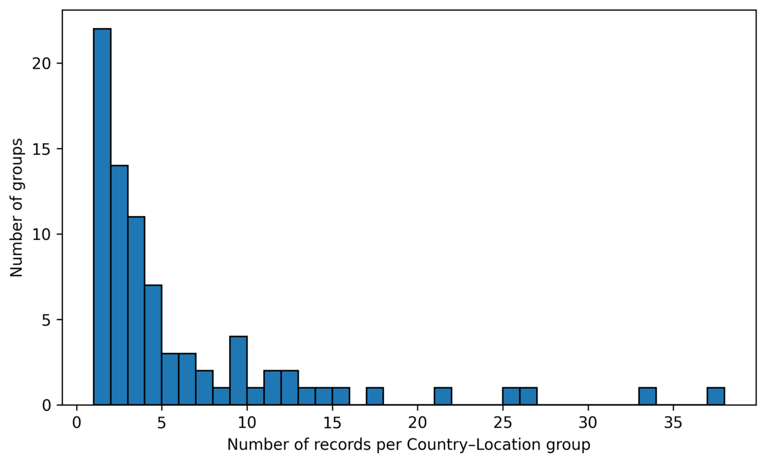
The cleaned dataset contained 459 records distributed across 81 Country–Location groups. The group sizes were uneven, ranging from 1 to 37 records, with a median of 3 records per group (Figure 12). Therefore, the LOLO results should be interpreted as a stricter external validation diagnostic rather than a direct replacement for random-split metrics.

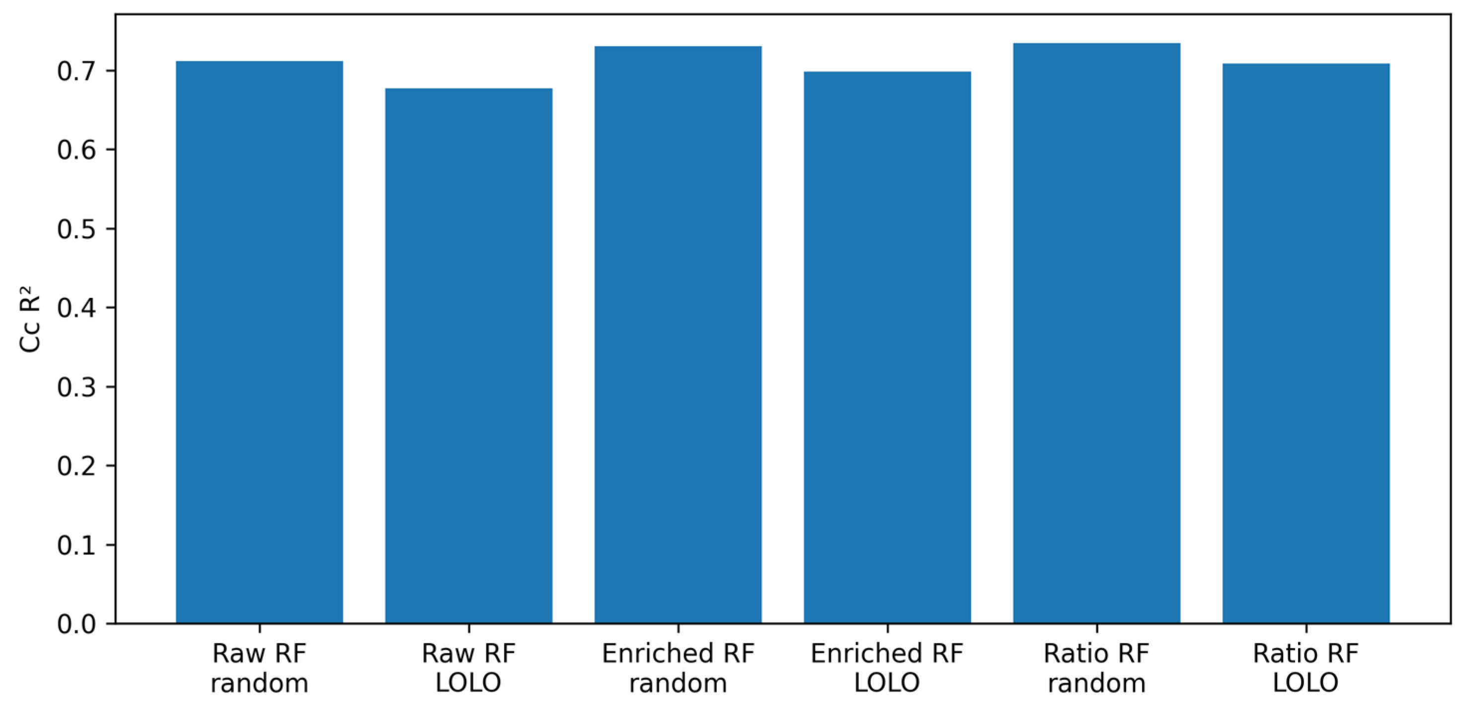
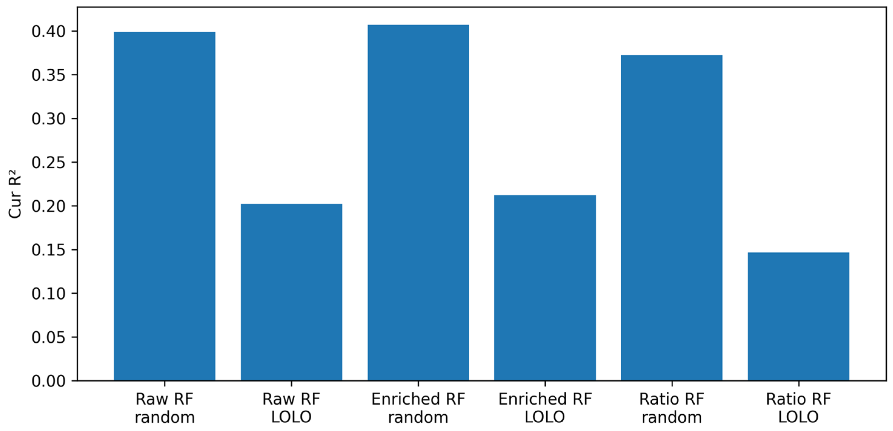
As shown in

Table 12. Random and leave-one-location-out validation performance for RF-based models.

Model	Validation	Cc R2	Cc RMSE	Cc MAE	Cur R2	Cur RMSE	Cur MAE	Violation (%)	Near-Violation (%)
RF raw	random 10-fold	0.712	0.3838	0.2583	0.399	0.0406	0.0313	0.000	10.022
RF enriched	random 10-fold	0.731	0.3711	0.2462	0.407	0.0403	0.0309	0.000	9.368
RF ratio	random 10-fold	0.734	0.3685	0.2324	0.372	0.0415	0.0307	0.000	11.547
RF raw	LOLO	0.677	0.4065	0.2788	0.202	0.0468	0.0360	0.000	9.150
RF enriched	LOLO	0.698	0.3929	0.2749	0.212	0.0465	0.0359	0.000	8.715
RF ratio	LOLO	0.709	0.3859	0.2547	0.147	0.0484	0.0373	0.000	11.983

, location-aware validation reduced predictive performance compared with random 10-fold cross-validation, particularly for Cur. For Cc, the RF models retained moderate transferability, with LOLO R² values between 0.677 and 0.709. The ratio-based RF formulation produced the highest LOLO R² for Cc, while the enriched RF model slightly improved performance relative to the raw-index model (Figure 13 and Figure 14).

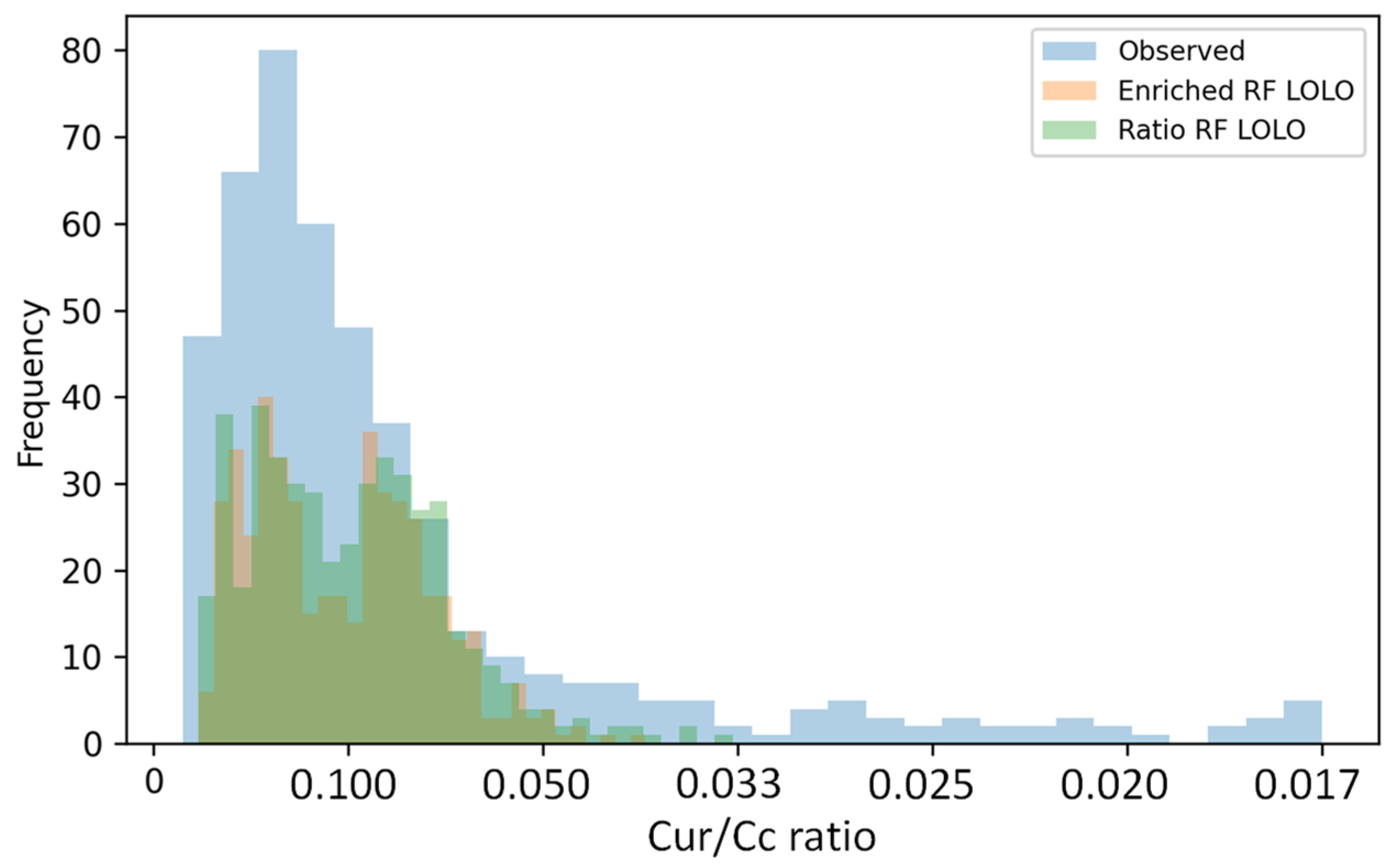
For Cur, LOLO performance remained weak, with R² values between 0.147 and 0.212. The enriched features provided only a small improvement over the raw inputs, while the ratio-based formulation ensured physically admissible predictions but did not improve the Cur accuracy (Figure 15 and Figure 16). The observed and predicted Cur/Cc distributions in Figure 17 further show that the models capture the central ratio range but compress part of the distributional variability.

5. Discussion

5.1. Comparison with Empirical Correlations

The cleaned CLAY/Cc/6/6203 subset spans a wide range of plasticities, states and compressibilities, making it suitable for benchmarking index-based prediction of Cc and Cur. The single-output and multi-output ensembles extend classical empirical correlations by capturing nonlinear interactions among LL, PI, w and e [2,3,4,5,7].

For Cc, the tree-based models explain about 60–65% of the test-set variance, with test R² values of approximately 0.61–0.64. This performance is favourable compared with traditional correlations based on LL, PI or e₀, such as those proposed by Skempton, Burland, Mesri and co-workers [2,3,4,34]. The improved performance reflects the ability of RF and XGB to represent nonlinear relationships between soil state and plasticity.

Cur remains less predictable from the same four inputs, with the best tree-based models achieving test R² values of about 0.29. This is consistent with previous empirical studies, where recompression indices show weaker and more scattered relationships than Cc [2,3,4]. Although the models improve on fixed-ratio assumptions, Cur inferred only from LL, PI, w and e should still be considered a screening-level estimate.

DNNs provided a useful benchmark. They slightly improved Cc prediction, with DNN_Cc reaching a test R² of about 0.69, but it did not improve Cur prediction. This suggests that higher model flexibility can improve Cc prediction to some extent but cannot overcome the information limits of index-only inputs for Cur [6,7,8,9,11,12,13,14,15,16,17,21,22].

5.2. Added Value of Multi-Output Modelling and Interpretability

Multi-output learning did not substantially improve marginal error metrics, but it improved the physical coherence of paired Cc–Cur predictions. The multi-output models produced no test-set cases violating Cur < Cc, and the predicted Cur/Cc ratios remained close to the observed central range. This is important because settlement calculations use Cc and Cur together, and physically inconsistent pairs can lead to unrealistic deformation estimates.

Interpretability also supports the engineering relevance of the models. The SHAP results show that e and w are the dominant predictors for Cc, while LL and PI play secondary roles. This agrees with the expected role of soil state in controlling compressibility. For Cur, SHAP effects are weaker and more diffuse, explaining why Cur is less accurately predicted under the index-only scenario.

Overall, multi-output tree ensembles provide a practical balance between accuracy, interpretability and physical consistency. They are simpler and more transparent than DNNs while still producing mechanically admissible paired predictions.

5.3. Implications for Practice

For Cc, the results indicate that RF, XGB and DNN models can provide useful preliminary estimates from LL, PI, w and e. These estimates may support early-stage settlement assessment, interpolation between limited oedometer tests, and sensitivity studies where full consolidation testing is not yet available.

For Cur, the predictions should be used more cautiously. The models provide physically coherent first-order estimates and avoid unrealistic Cur ≥ Cc outcomes, but their modest R² values show that they should not replace project-specific consolidation testing in serviceability-sensitive designs.

From a practical implementation perspective, RF and XGB are attractive because they require only routine index properties and can be interpreted using SHAP. DNNs may slightly improve Cc accuracy but are less transparent and do not improve Cur prediction. Therefore, multi-output tree ensembles appear to be the most suitable option when interpretability, robustness and physical consistency are required.

5.4. Implications of the Physics-Guided Experiment

The physics-guided experiment shows that simple geotechnical feature enrichment can improve predictive accuracy. Adding PL, LI, w/LL, w/e and PI/LL increased the accuracy of the RF model for both Cc and Cur, indicating that soil-mechanics-based feature engineering can add useful information beyond the raw index properties [35,36,37].

The ratio-based transformation also provides a useful physical constraint. By modelling Cur/Cc, the framework guarantees positive and mechanically admissible predictions with Cur < Cc. However, the constrained formulation did not improve the Cur accuracy compared with the enriched RF model. This confirms that physical constraints can prevent impossible outputs but cannot replace missing geotechnical descriptors [38,39,40].

For engineering use, the enriched RF model is preferable when point-prediction accuracy is the main objective, while the ratio-based model is preferable when physical admissibility of the Cc–Cur pair is the priority. The four-variable empirical equations provide an additional transparent tool for preliminary assessment, but their use should remain limited to early-stage or low-risk applications.

5.5. Limitations and Future Work

The main limitation of this study is the restricted input space. The models use only LL, PI, w and e, which are practical and widely available but do not fully describe the mechanisms controlling clay compressibility. This limitation is most important for Cur, which cannot be reliably constrained from index properties alone.

A second limitation is the heterogeneous nature of the CLAY/Cc/6/6203 database. The records come from different regions, laboratories, sampling conditions and testing procedures. Although data cleaning reduced obvious inconsistencies, residual variability remains and may affect model transferability.

The LOLO validation provides a stricter assessment of generalisation than random splitting, but Country–Location groups are only an approximate proxy for true geological or project-level independence. Future datasets should include site IDs, geological units, sampling depth, depositional environment and laboratory programme metadata to support stronger grouped validation.

The uncertainty estimates should also be interpreted carefully. Bootstrap intervals provide comparative information about model variability, but they are not fully calibrated design bounds. Therefore, the proposed models should complement, not replace, targeted oedometer testing and engineering judgement.

Future work should combine routine index properties with stress-history, geological, mineralogical and microstructural descriptors. Probabilistic models, calibrated prediction intervals, and hybrid physics–ML approaches using full oedometer response curves may further improve the reliability of Cc–Cur prediction. Overall, the present study provides a reproducible benchmark for index-only prediction. Cc can be estimated with useful preliminary accuracy, while Cur remains a screening-level parameter unless additional descriptors are available.

6. Conclusions

This study developed an index-only machine learning framework for the joint prediction of the compression index (Cc) and recompression index (Cur) of natural clays using four routine properties: LL, PI, e, and w. A cleaned subset of 459 records from the CLAY/Cc/6/6203 database was used to compare single-output, multi-output, geotechnically enriched, physically constrained, and empirical formulations.

The results show that Cc can be predicted with useful preliminary accuracy from routine index properties. Under random-split evaluation, baseline models achieved test R² values of approximately 0.61–0.70 for Cc, and performance improved further when geotechnically meaningful derived features were added. This confirms that LL, PI, e, and w provide useful information for estimating virgin compression behaviour, although the highest Cc values remained more difficult to capture.

Cur was substantially less predictable. Tree-based models achieved random-split Cur test R² values of about 0.29, and performance decreased further under leave-one-location-out validation. This indicates that Cur should be treated as a screening-level estimate when only LL, PI, e, and w are available, because important recompression controls are not explicitly represented in the input space.

The geotechnically enriched Random Forest provided the best overall point-prediction performance, while the physically constrained Cur/Cc ratio formulation ensured mechanically admissible predictions with positive values and Cur < Cc. However, the constraint improved admissibility rather than recovering the missing information required for accurate Cur prediction. SHAP interpretation confirmed that e and w were the dominant contributors to Cc prediction, whereas Cur showed a weaker and more diffuse dependence on the available inputs.

Location-aware validation demonstrated the importance of grouped evaluation in geotechnical ML. Random splits can overestimate transferability when related records from the same location appear in both the training and testing sets. Cc retained moderate transferability across locations, whereas Cur performance deteriorated markedly, confirming its stronger site dependence.

Overall, the proposed workflow can support the preliminary estimation of clay compressibility from routine index data, particularly for Cc. The practical four-variable empirical equations also provide a transparent benchmark for direct engineering use. However, Cur predictions from LL, PI, e, and w alone should not be used as design-grade replacements for project-specific oedometer testing. Future databases should include stress-history, geological, mineralogical, and microstructural descriptors to improve the transferable prediction of recompression behaviour.

References

1. Terzaghi, K.; Peck, R.B.; Mesri, G. Soil Mechanics in Engineering Practice, 3rd ed.; Wiley: New York, NY, USA, 1996. [Google Scholar]
2. Skempton, A.W.; Jones, O.T. Notes on the compressibility of clays. Q. J. Geol. Soc. 1944, 100, 119–135. [Google Scholar] [CrossRef] [Scilit]
3. Burland, J.B. On the compressibility and shear strength of natural clays. Géotechnique 1990, 40, 329–378. [Google Scholar] [CrossRef] [Scilit]
4. Mesri, G.; Rokhsar, A.; Bohor, B.F. Composition and compressibility of typical samples of Mexico City clay. Géotechnique 1975, 25, 527–554. [Google Scholar] [CrossRef] [Scilit]
5. Chong, S.H.; Santamarina, J.C. Soil compressibility models for a wide stress range. J. Geotech. Geoenvironmental Eng. 2016, 142, 06016003. [Google Scholar] [CrossRef] [Scilit]
6. Ching, J.; Phoon, K.K. Transformations and correlations among some clay parameters—The global database. Can. Geotech. J. 2014, 51, 663–685. [Google Scholar] [CrossRef] [Scilit]
7. Ching, J.; Phoon, K.K. Correlations among some clay parameters—The multivariate distribution. Can. Geotech. J. 2014, 51, 686–704. [Google Scholar] [CrossRef] [Scilit]
8. Ching, J.; Phoon, K.K.; Wu, C.T. Data-centric quasi-site-specific prediction for compressibility of clays. Can. Geotech. J. 2022, 59, 2033–2049. [Google Scholar] [CrossRef] [Scilit]
9. Ching, J.; Phoon, K.K.; Pan, Y.K.; Zhang, W.; Li, J. Introduction to CLAY-Cc/6/6203 database. Geod. AI 2024, 1, 100005. [Google Scholar] [CrossRef] [Scilit]
10. Phoon, K.K. Trustworthy data-centric geotechnics. Geod. AI 2024, 1, 100008. [Google Scholar] [CrossRef] [Scilit]
11. Bui, D.T.; Nhu, V.H.; Hoang, N.D. Prediction of soil compression coefficient for urban housing project using a novel integration machine learning approach of swarm intelligence and multilayer perceptron neural network. Adv. Eng. Inform. 2018, 38, 593–604. [Google Scholar] [CrossRef] [Scilit]
12. Qiu, J.; Ohl, J.; Tran, T.T. Predicting clay compressibility for foundation design with high reliability and safety: A geotechnical engineering perspective using artificial neural network and five metaheuristic algorithms. Reliab. Eng. Syst. Saf. 2024, 243, 109827. [Google Scholar] [CrossRef] [Scilit]
13. Long, T.; He, B.; Ghorbani, A.; Khatami, S.M.H. Tree-based techniques for predicting the compression index of clayey soils. J. Soft Comput. Civ. Eng. 2023, 7, 52–67. [Google Scholar] [CrossRef]
14. Wu, H.; Zhang, Z.; Dias, D. Prediction on compression indicators of clay soils using XGBoost with Bayesian optimization. J. Cent. South Univ. 2024, 31, 3914–3929. [Google Scholar] [CrossRef] [Scilit]
15. Díaz, E.; Spagnoli, G. A super-learner machine learning model for a global prediction of compression index in clays. Appl. Clay Sci. 2024, 249, 107239. [Google Scholar] [CrossRef] [Scilit]
16. Ge, Q.; Xia, Y.; Shu, J.; Li, J.; Sun, H. Explainable ensemble learning approaches for predicting the compression index of clays. J. Mar. Sci. Eng. 2024, 12, 1701. [Google Scholar] [CrossRef] [Scilit]
17. Baghbani, A.; Kiany, K.; Abuel-Naga, H.; Lu, Y. Predicting the compression index of clayey soils using a hybrid genetic programming and XGBoost model. Appl. Sci. 2025, 15, 1926. [Google Scholar] [CrossRef] [Scilit]
18. Breiman, L. Random forests. Mach. Learn. 2001, 45, 5–32. [Google Scholar] [CrossRef] [Scilit]
19. Friedman, J.H. Greedy function approximation: A gradient boosting machine. Ann. Stat. 2001, 29, 1189–1232. [Google Scholar] [CrossRef] [Scilit]
20. Lundberg, S.M.; Lee, S.I. A unified approach to interpreting model predictions. In Advances in Neural Information Processing Systems, 2nd ed.; Curran Associates: New York, NY, USA, 2017; Volume 30, pp. 4765–4774. [Google Scholar]
21. Goodfellow, I.; Bengio, Y.; Courville, A. Deep Learning; MIT Press: Cambridge, MA, USA, 2016. [Google Scholar]
22. Zhang, W.; Li, H.; Li, Y.; Liu, H.; Chen, Y.; Ding, X. Application of deep learning algorithms in geotechnical engineering: A short critical review. Artif. Intell. Rev. 2021, 54, 5633–5673. [Google Scholar] [CrossRef] [Scilit]
23. Kordnaeij, A.; Kalantary, F.; Kordtabar, B.; Mola-Abasi, H. Prediction of recompression index using GMDH-type neural network based on geotechnical soil properties. Soils Found. 2015, 55, 1335–1345. [Google Scholar] [CrossRef] [Scilit]
24. Kootahi, K. Simple index tests for assessing the recompression index of fine-grained soils. J. Geotech. Geoenviron. Eng. 2017, 143, 06016027. [Google Scholar] [CrossRef] [Scilit]
25. Kurnaz, T.F.; Dagdeviren, U.; Yildiz, M.; Ozkan, O. Prediction of compressibility parameters of the soils using artificial neural network. SpringerPlus 2016, 5, 1801. [Google Scholar] [CrossRef] [Scilit] [PubMed]
26. Zhang, P.; Yin, Z.Y.; Sheil, B. Interpretable data-driven constitutive modelling of soils with sparse data. Comput. Geotech. 2023, 160, 105511. [Google Scholar] [CrossRef] [Scilit]
27. Kiany, K.; Baghbani, A.; Abuel-Naga, H.; Yi, L. Novel integration of FEM, Physics-Informed Neural Networks, and explainable Metaheuristics for retaining wall analysis. Int. J. Geotech. Eng. 2025, 19, 813–831. [Google Scholar] [CrossRef] [Scilit]
28. Baghbani, A.; Abuel-Naga, H.; Shirkavand, D. Accurately predicting quartz sand thermal conductivity using machine learning and grey-box AI models. Geotechnics 2023, 3, 638–660. [Google Scholar] [CrossRef] [Scilit]
29. Yuan, B.; Choo, C.S.; Yeo, L.Y.; Wang, Y.; Yang, Z.; Guan, Q.; Suryasentana, S.; Choo, J.; Shen, H.; Megia, M.; et al. Physics-informed machine learning in geotechnical engineering: A direction paper. Geomech. Geoengin. 2025, 20, 1128–1159. [Google Scholar] [CrossRef] [Scilit]
30. Bozorgzadeh, N.; Feng, Y. Evaluation structures for machine learning models in geotechnical engineering. Georisk Assess. Manag. Risk Eng. Syst. Geohazards 2024, 18, 52–59. [Google Scholar] [CrossRef] [Scilit]
31. Baghbani, A.; Soltani, A.; Kiany, K.; Daghistani, F. Predicting the strength performance of hydrated-lime activated rice husk ash-treated soil using two grey-box machine learning models. Geotechnics 2023, 3, 894–920. [Google Scholar] [CrossRef] [Scilit]
32. Jais, I.K.M.; Ismail, A.R.; Nisa, S.Q. Adam optimization algorithm for wide and deep neural network. Knowl. Eng. Data Sci. 2019, 2, 41–46. [Google Scholar] [CrossRef] [Scilit]
33. Kingma, D.P.; Ba, J. Adam: A method for stochastic optimization. In Proceedings of the 3rd International Conference for Learning Representations, San Diego, CA, USA, 7–9 May 2015. [Google Scholar]
34. Aminaee, A.; Ardakani, A.; Baghbani, A.; Abuel-Naga, H.; Daghistani, F. Hybrid ML–XAI Framework for Predicting and Interpreting the Strength of Lime–Silica Fume Stabilized Clay for Sustainable Construction Applications. Buildings 2026, 16, 953. [Google Scholar] [CrossRef] [Scilit]
35. Azzouz, A.S.; Krizek, R.J.; Corotis, R.B. Regression analysis of soil compressibility. Soils Found. 1976, 16, 19–29. [Google Scholar] [CrossRef] [Scilit] [PubMed]
36. Yang, S.; Lin, K.; Zhou, A. Evaluating Water Retention and Hydraulic Conductivity Properties Based on the Richardson–Richards Equation Using Progressive Training and Trainable Weights. Int. J. Numer. Anal. Methods Geomech. 2026, 50, 1045–1060. [Google Scholar]
37. Li, D.; Cao, Y.; Huang, S.; Cui, Y.; Wei, X.; Cao, H.; Wang, C. Lagged backward-compatible physics-informed neural networks for unsaturated soil consolidation analysis. Can. Geotech. J. 2026, 63, 1–28. [Google Scholar] [CrossRef] [Scilit]
38. Li, D.; Jiang, Z.; Tian, K.; Ji, R. Prediction of hydraulic conductivity of sodium bentonite GCLs by machine learning approaches. Environ. Geotech. 2025, 12, 154–173. [Google Scholar] [CrossRef] [Scilit]
39. Li, D.; Jiang, Z.; Tian, K.; Ji, R. Estimation of the hydraulic conductivity of bentonite–polymer GCLs with machine learning techniques. Environ. Geotech. 2025, 12, 433–451. [Google Scholar] [CrossRef] [Scilit]
40. Cheng, K.; Ziotopoulou, K. Machine Learning in Geotechnical Engineering: A Survey of Progress, Gaps, and Opportunities. Int. J. Geomech. 2026, 26, 03126001. [Google Scholar] [CrossRef] [Scilit]
Figure 1. Pearson correlation matrix between index properties (LL, PI, w, e) and compressibility parameters (Cc, Cur) for the cleaned Cc–Cur database.
Applsci 16 07068 g001
Figure 2. Univariate distributions of LL, PI, w, e, Cc, and Cur for the cleaned Cc–Cur subset: (a) LL, (b) PI, (c) w, (d) e, (e) Cc, and (f) Cur.
Applsci 16 07068 g002
Figure 3. (a) Relationship between measured Cc and Cur and (b) distribution of the Cur/Cc ratio for the global clay dataset.
Applsci 16 07068 g003
Figure 4. Leave-one-location-out sensitivity to small Country–Location groups. Pooled R2 values are shown for all groups, after excluding singleton groups and after excluding groups with one to three records.
Applsci 16 07068 g004
Figure 5. Predicted versus observed Cc and Cur for RF, XGB and DNN single-output models, showing 10-fold cross-validation (train) and independent test-set performance.
Applsci 16 07068 g005
Figure 6. Predicted versus observed Cc and Cur for multi-output models (MO_RF, MO_XGB, DNN_MO).
Applsci 16 07068 g006
Figure 7. Global SHAP beeswarm plots for the single-output XGBoost model: (a) Cc and (b) Cur. Features are ordered by decreasing mean absolute SHAP value.
Applsci 16 07068 g007
Figure 8. Global SHAP beeswarm plots for the multi-output Random Forest (MO_RF): (a) Cc and (b) Cur.
Applsci 16 07068 g008
Figure 9. SHAP analysis for XGB_Cc: dependence plots for selected inputs (e, w, PI and LL).
Applsci 16 07068 g009
Figure 10. SHAP analysis for XGB_Cur: dependence plots for selected inputs (e, w, PI, and LL).
Applsci 16 07068 g010
Figure 11. Admissibility map in e–w space for coupled outputs (MO-RF).
Applsci 16 07068 g011
Figure 12. Distribution of group sizes used in leave-one-location-out validation.
Applsci 16 07068 g012
Figure 13. Random versus location-aware R2 for Cc.
Applsci 16 07068 g013
Figure 14. LOLO predicted versus observed Cc for the enriched RF model.
Applsci 16 07068 g014
Figure 15. Random versus location-aware R2 for Cur.
Applsci 16 07068 g015
Figure 16. LOLO predicted versus observed Cur for the enriched RF model.
Applsci 16 07068 g016
Figure 17. Observed and predicted Cur/Cc ratio distributions.
Applsci 16 07068 g017