Predictive Maintenance of DC Fast-Charging Stations Using Unsupervised Anomaly Detection

Abstract

The reliability of electric vehicle fast-charging infrastructure is becoming increasingly critical as deployment accelerates and the number of unavailable charging points grows. This work presents an unsupervised anomaly detection framework aimed at supporting predictive maintenance in DC fast-charging stations. The approach uses real minute-resolution operational data from a real charging station, including active, reactive and apparent power, power factor, phase power measurements and charger-side power measurements. Three complementary anomaly detection models were designed to capture different abnormal operating conditions: deviations in consumption patterns, efficiency losses between charger and grid analyser measurements, and phase imbalance in three-phase operation. Local Outlier Factor and Isolation Forest algorithms were integrated into an automated monitoring pipeline. Since labelled fault data were not available, validation was based on controlled injection of synthetic anomalies into real test signals, including physically coherent power disturbances, sensor or communication inconsistencies, progressive efficiency degradation and phase imbalance events. The results show that the framework is effective for detecting anomaly families that produce clear or sustained deviations, while more subtle temporal behaviours remain more challenging. Overall, the proposed framework provides a practical condition monitoring and early-warning approach that can support predictive maintenance decisions in DC charging infrastructure, while further temporal modelling is required for explicit degradation forecasting.

1. Introduction

The deployment of electric vehicle (EV) charging infrastructure is accelerating as part of the transition towards low-emission mobility. According to the International Energy Agency, the global stock of publicly accessible charging points exceeded 7 million by the end of 2025, after nearly 1.8 million public chargers were added during that year, representing an increase of more than 33% compared with 2024 [1]. However, the expansion of installed charging infrastructure does not by itself guarantee service availability. As charging networks grow, ensuring the reliability, operational safety and maintainability of charging stations becomes increasingly important.

This issue is particularly relevant for DC fast-charging stations, which integrate power conversion, charging control, protection and communication functions within the infrastructure itself [2]. Unlike AC charging points, where the vehicle’s on-board charger largely determines the electrical charging behaviour, DC fast chargers actively regulate the charging process. Consequently, abnormal electrical behaviour observed in DC fast-charging stations is more directly related to the infrastructure under monitoring and may provide valuable information for maintenance and fault diagnosis.

Predictive maintenance aims to monitor the condition of equipment during operation in order to anticipate faults before they lead to service interruption [3,4]. Within this framework, anomaly detection [5] plays a central role by identifying deviations from normal operating behaviour in multivariate operational data. In DC fast-charging stations, such deviations may appear as abnormal power consumption patterns, efficiency losses between measurement points, phase imbalance, measurement inconsistencies or unexpected transient behaviour.

Despite the potential of anomaly detection for charging infrastructure, its deployment in real operational environments remains challenging. Documented fault data are scarce, heterogeneous and rarely available in sufficient quantity for supervised learning. In addition, the electrical behaviour of charging stations is multivariate, nonlinear and affected by changing operating conditions. These limitations motivate the use of unsupervised anomaly detection methods, which can learn normal operating patterns without requiring labelled examples of faults.

This work presents an unsupervised anomaly detection framework for DC fast-charging stations using real operational data from a real charging station. The proposed approach focuses on three complementary anomaly categories: abnormal electrical consumption behaviour, efficiency deviations between charger-side and grid-side power measurements, and phase imbalance in three-phase operation. Since no labelled dataset of real faults was available, the validation strategy is based on the controlled injection of synthetic anomalies into real test signals. This allows model performance to be evaluated under known abnormal conditions while preserving the variability and temporal structure of real operational data.

The main contribution of this work is the development and validation of a practical data-driven framework for condition monitoring and early anomaly detection in DC fast-charging infrastructure. The methodology combines real monitoring data, unsupervised machine learning models and synthetic anomaly injection to identify abnormal operating periods that may support predictive maintenance decisions and technical diagnosis in operational EV charging environments. In this context, the framework focuses on anomaly-based monitoring and maintenance prioritisation, while explicit fault prognosis and remaining useful life estimation remain outside the scope of the present study.

2. Related Work

Anomaly detection in EV charging infrastructure has been addressed using different methodological approaches, ranging from deterministic rules and statistical monitoring to machine learning and deep learning techniques [6]. The choice of method depends strongly on the availability of labelled fault data, the complexity of the monitored system and the type of anomalies to be detected.

Early approaches in charging infrastructure and related electrical systems often relied on deterministic rules, fixed thresholds or statistical monitoring techniques. These methods typically define limits on variables such as voltage, current, power, temperature or efficiency indicators [7]. Statistical tools such as z-score analysis, interquartile range methods and control charts have also been used to identify observations that deviate from expected operating ranges. Their main advantages are simplicity, interpretability and low computational cost. However, their performance is limited when the monitored system presents nonlinear behaviour, variable operating regimes or strong interactions between variables. In DC fast-charging stations, where operating conditions can change significantly between charging sessions, fixed thresholds may generate false alarms or fail to detect subtle degradation patterns.

Supervised machine learning methods have also been explored for fault and anomaly detection by formulating the problem as a classification task between normal and abnormal states. Algorithms such as support vector machines, random forests, gradient boosting, k-nearest neighbours and neural networks can achieve high detection performance when representative labelled data are available. Nevertheless, this requirement is a major limitation in real charging infrastructure. Faults are relatively rare, heterogeneous and often poorly documented, while many abnormal behaviours may not have occurred previously in the monitored system. As a result, purely supervised approaches are difficult to deploy in operational environments where labelled anomaly datasets are not available.

Unsupervised anomaly detection has therefore become a particularly relevant approach for EV charging applications. These methods do not require labelled fault examples and instead learn the structure of normal operation, identifying observations that deviate from the expected data distribution. Classical unsupervised algorithms such as Isolation Forest, Local Outlier Factor, One-Class SVM, clustering-based methods and dimensionality reduction approaches have been widely used for this purpose [8,9]. Isolation Forest detects anomalies according to how easily each observation can be isolated through random partitions of the feature space, whereas Local Outlier Factor identifies samples located in regions of lower local density compared with their neighbours. These methods are attractive for charging infrastructure because they offer a practical compromise between computational cost, interpretability and applicability to real operational data.

Recent work has also incorporated explainability into anomaly detection for EV charging stations. In operational maintenance contexts, an anomaly label alone is often insufficient since technical teams require additional information to understand which variables contributed to the abnormal behaviour and to prioritise interventions. For this reason, feature importance techniques and explainable anomaly detection methods have been proposed to improve the diagnostic value of machine learning-based monitoring systems [10].

In parallel, deep learning methods have increasingly been applied to anomaly detection and monitoring in EV charging and smart-grid environments [11,12,13,14,15,16]. Autoencoders, convolutional neural networks, recurrent neural networks and LSTM-based architectures can model nonlinear relationships and temporal dependencies in multivariate time series. These approaches are especially useful when large volumes of data are available and the objective is to learn complex representations of normal operation. However, they generally require more data, greater computational resources and more careful tuning than classical unsupervised methods. In addition, their reduced interpretability may limit adoption in maintenance-oriented applications unless combined with explanation mechanisms.

Another relevant research line addresses anomaly detection from a cybersecurity perspective [8,12,17,18]. Charging stations are cyber–physical systems connected to vehicles, back-end platforms and, in some cases, grid services. This exposes them to attacks such as manipulation of charging profiles, false data injection, denial-of-service events or communication tampering. Some works propose intrusion detection systems that combine forecasting models, supervised classifiers and novelty detection to identify both known and previously unseen attacks during charging sessions. Although this perspective is not identical to predictive maintenance, it is closely related because cyber-induced deviations and technical faults may both appear as abnormal patterns in operational data.

Despite these advances, several challenges remain open. First, the generalisation of anomaly detection models across different charger types, manufacturers, power levels, vehicles and operating conditions is still limited. Second, the absence of labelled real faults complicates objective validation and comparison between methods. Third, the choice of detection thresholds is often empirical and sensitive to data drift, which may increase false positives over time. Finally, many existing approaches focus on generic session-level anomalies or cybersecurity events, while fewer works address infrastructure-oriented indicators such as efficiency deviations between measurement points or phase imbalance in three-phase DC fast-charging operation.

In this context, the present work focuses on unsupervised anomaly detection for DC fast-charging infrastructure using real operational data. Unlike approaches based only on generic charging session indicators, the proposed framework combines classical unsupervised models with domain-specific monitoring variables related to consumption behaviour, efficiency and phase balance. In addition, the use of controlled synthetic anomaly injection enables quantitative validation in the absence of labelled real faults, which remains one of the main limitations for deploying anomaly detection systems in real charging infrastructure.

3. Materials and Methods

3.1. Dataset

The dataset used in this study was collected from the Smart Mobility Lab of the Instituto Tecnológico de la Energía (ITE) [19]. It includes several electric vehicle charging stations with different power levels and technologies. However, this work focuses exclusively on the DC fast-charging station since, in this type of infrastructure, the main power conversion, charging control, regulation, protection and communication functions are integrated into the charging station itself. Therefore, the electrical behaviour observed during charging is more directly related to the infrastructure under monitoring than in AC charging, where the vehicle on-board charger has a dominant influence on the charging profile.

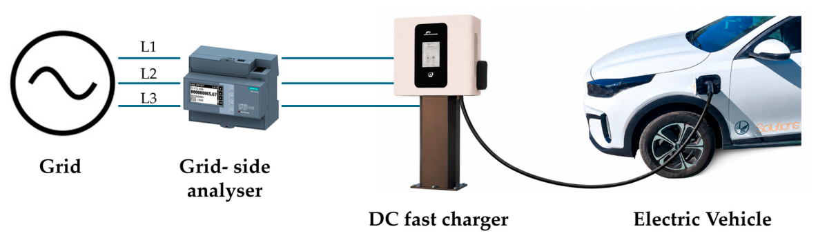
The monitored DC charging point corresponds to a Power Electronics NBW30 fast charger (Power Electronics España S.L., Llíria, Spain), with a rated power of 30 kW [20]. The station is supplied from a three-phase grid and is monitored through two complementary measurement points, as shown in Figure 1. The first measurement point is located at the grid side and corresponds to a Siemens PAC2200 network analyser (Siemens AG, Munich, Germany), which provides active power, reactive power, apparent power, power factor and active power per phase. The second measurement point is located at the charger side and provides the active power reported by the charging management system. All measurements are recorded with a one-minute temporal resolution. The availability of these two measurement points enables both the characterisation of the electrical behaviour of the charger and the comparison between grid-side and charger-side power measurements.

Table 1. Variables included in the dataset.

Variable	Description	Source
Active power	Total active power consumed by the DC charger	Grid-side analyser
Reactive power	Total reactive power associated with charger operation	Grid-side analyser
Apparent power	Total apparent power	Grid-side analyser
Power factor	Ratio between active and apparent power	Grid-side analyser
Phase active power L1	Active power measured in phase L1	Grid-side analyser
Phase active power L2	Active power measured in phase L2	Grid-side analyser
Phase active power L3	Active power measured in phase L3	Grid-side analyser
Charger-side active power	Active power reported by the charging station	Charging management system

summarises the variables included in the dataset.

The dataset covers approximately two years of operation of the monitored DC fast-charging station and includes around 100 active DC fast-charging sessions. This number of charging events reflects the operational context of the installation, which corresponds to a private company charging point where additional lower-power chargers are also available and are more frequently used for regular charging needs. Consequently, active DC charging represents only a limited fraction of the monitored period. However, the station was continuously monitored at one-minute resolution, and the complete non-charging and standby operation was also recorded throughout the observation period. This is relevant for the proposed framework because non-charging consumption is explicitly modelled as an independent monitoring task aimed at detecting abnormal standby behaviour, residual consumption, unexpected power peaks and unregistered charging activity. Since labelled real faults were not available, these operational data were used as the basis for the controlled injection of synthetic anomalies during the validation stage.

3.2. Proposed Anomaly Detection Framework

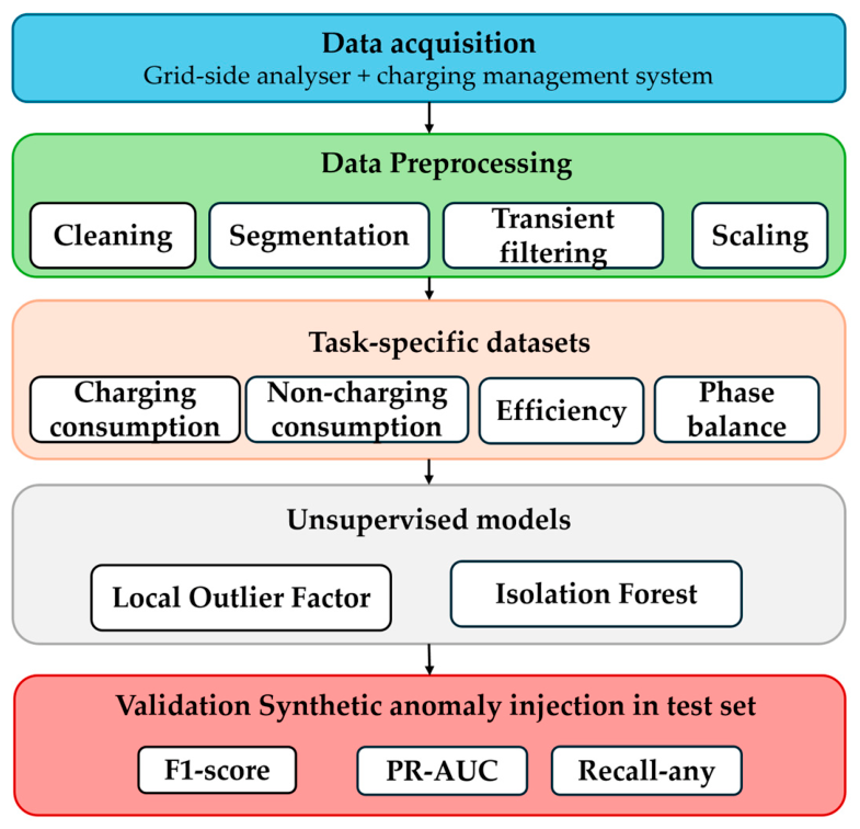
The proposed framework (Figure 2) is designed to detect abnormal operating conditions in DC fast-charging infrastructure using real operational measurements and unsupervised learning models. Based on the available electrical variables, three complementary anomaly detection tasks are defined: consumption anomaly detection, efficiency deviation detection and phase imbalance anomaly detection. Each task focuses on a different aspect of the charging process and is intended to capture a different family of abnormal behaviours. The complete processing path consists of raw data harmonisation, operating-state segmentation, task-specific feature construction, model training on historical data, anomaly scoring and validation through synthetic anomaly injection.

3.2.1. Methodological Formulation

The proposed framework is formulated as an unsupervised anomaly detection problem for condition monitoring of DC fast-charging infrastructure. Let $X=\left\{x_t\right\}$ denote the multivariate operational time series collected from the charging station, where each $x_t$ contains the electrical measurements recorded at timestamp $t$. Since labelled fault examples are not available, the objective is to learn the normal operating behaviour of the charger from historical data and to identify observations that deviate from this behaviour.

After defining the monitoring tasks, each task is associated with a specific input representation. For the consumption task, the feature vector is built from the main electrical consumption variables. For the efficiency deviation task, the representation is based on the relationship between charger-side and grid-side active power measurements. For the phase imbalance task, the representation is based on the distribution of active power among the three phases.

An unsupervised model then assigns an anomaly score $s_{t,k,m}=f_{k,m}\left(z_t^{\left(k\right)}\right)$, where $k$ denotes the monitoring task and $m\in \{\mathrm{L}\mathrm{O}\mathrm{F},\mathrm{I}\mathrm{F}\}$ denotes the selected unsupervised model.

More formally, for each monitoring task $k$, the raw measurement vector $x_t$ is transformed into a task-specific input vector:

$$z_t^{\left(k\right)}=g_k\left(x_t\right)$$

(1)

where $g_k(\cdot )$ represents the feature construction function associated with the corresponding monitoring task. The anomaly score is then obtained using an unsupervised detector:

$$s_{t,k,m}=f_{k,m}\left(z_t^{\left(k\right)}\right),m\in \{\mathrm{L}\mathrm{O}\mathrm{F},\mathrm{I}\mathrm{F}\}$$

(2)

where $m$ denotes the anomaly detection model used for task $k$. For consistency between models, the scores are expressed so that larger values indicate a greater degree of abnormality; when necessary, the sign of the original model output is reversed.

The threshold for task $k$ and model $m$ is then determined from the training score distribution as:

$${\tau }_{k,m}=Q_{1-{\alpha }_{k,m}}\left({\left\{s_{i,k,m}^{\mathrm{t}\mathrm{r}\mathrm{a}\mathrm{i}\mathrm{n}}\right\}}_{i=1}^{N_{\mathrm{t}\mathrm{r}\mathrm{a}\mathrm{i}\mathrm{n}}}\right),$$

(3)

where $Q_{1-{\alpha }_{k,m}}$ is the empirical quantile of order $1-{\alpha }_{k,m}$ of the training anomaly score distribution and ${\alpha }_{k,m}$ is the contamination factor defined for task $k$ and model $m$.

Thus, approximately the fraction ${\alpha }_{k,m}$ of the training observations with the highest anomaly scores lies above the threshold. The threshold is fixed after model fitting and subsequently applied to unseen test or operational samples.

Finally, the anomaly flag is obtained by applying a task- and model-specific operational threshold:

$$a_{t,k,m}=\left\{\begin{array}{cc}1,& s_{t,k,m}\ge {\tau }_{k,m}\\ 0,& s_{t,k,m}<{\tau }_{k,m}\end{array}\right.$$

(4)

where $a_{t,k,m}=1$ denotes an anomalous observation. Under this formulation, the same anomaly detection logic is applied to the different monitoring tasks, while the input representation $z_t^{\left(k\right)}$, the scoring function $f_{k,m}$, the contamination factor ${\alpha }_{k,m}$ and the threshold ${\tau }_{k,m}$ are defined for each task and model.

3.2.2. Consumption Anomaly Detection

The consumption anomaly detection task aims to identify abnormal electrical behaviour in the DC fast-charging station using the main grid-side variables: active power, reactive power, apparent power and power factor. These variables jointly characterise the global electrical operation of the charger and allow the detection of deviations such as unexpected power drops, transient peaks, unstable charging profiles or inconsistencies between electrical magnitudes.

Formally, for each operating regime $r\in \{\mathrm{c}\mathrm{h},\mathrm{n}\mathrm{c}\}$, the consumption-monitoring input vector at timestamp $t$ is defined as:

$${\mathrm{z}}_t^{\left(C,r\right)}={\left[{\tilde{P}}_t,{\tilde{Q}}_t,{\tilde{S}}_t,{\widetilde{PF}}_t,{\tilde{P}}_{L1,t},{\tilde{P}}_{L2,t},{\tilde{P}}_{L3,t}\right]}^T,t\in {\mathcal{T}}_r,r\in \{\mathrm{c}\mathrm{h},\mathrm{n}\mathrm{c}\}$$

(5)

where $P_t$, $Q_t$, $S_t$, $P{F}_t$, $P_{L1,t}$, $P_{L2,t}$, and $P_{L3,t}$ denote the original active power, reactive power, apparent power, power factor, and active power measured in phases L1, L2, and L3, respectively. The tilde indicates the corresponding scaled variable used as model input, ${\mathcal{T}}_r$ is the set of timestamps belonging to operating regime $r$, and $\mathrm{c}\mathrm{h}$ and $\mathrm{n}\mathrm{c}$ denote active charging and non-charging operations, respectively.

For each operating regime and model $m\in \{\mathrm{L}\mathrm{O}\mathrm{F},\mathrm{I}\mathrm{F}\}$, an anomaly score is computed as:

$$s_{t,C,r,m}=f_{C,r,m}\left({\mathrm{z}}_t^{\left(C,r\right)}\right)$$

(6)

The corresponding anomaly flag is then obtained as:

$$a_{t,C,r,m}=\left\{\begin{array}{cc}1,& \mathrm{if}{s}_{t,C,r,m}\ge {\tau }_{C,r,m},\\ 0,& \mathrm{otherwise}.\end{array}\right.$$

(7)

where ${\tau }_{C,r,m}$ is the operational threshold associated with the selected model and contamination factor. Under this formulation, a consumption anomaly is not defined by a fixed threshold on a single electrical variable but by the joint deviation of the multivariate consumption vector from the normal operating distribution learned for the corresponding operating regime.

Since the station behaviour differs substantially between active charging and idle operation, two separate models are used: one for charging periods and one for non-charging periods. This separation prevents the model from mixing operating regimes with different normal patterns. For instance, high active power is expected during charging but anomalous in standby, whereas very low power is normal during idle operation but may indicate an interruption during charging.

The charging model therefore focuses on deviations in the power profile during energy delivery, while the non-charging model detects abnormal standby behaviour, such as residual consumption, unexpected peaks or unregistered charging activity. Together, both models provide a general monitoring layer for identifying abnormal consumption patterns in different operating states of the DC charger.

3.2.3. Efficiency Deviation Detection

The efficiency deviation detection task analyses the relationship between the active power reported by the charging station and the active power measured at the grid-side analyser. This relationship is represented by an efficiency-related indicator defined as:

$$\mathsf{\eta }(t)={\displaystyle \frac{P_{\mathrm{c}\mathrm{h}\mathrm{a}\mathrm{r}\mathrm{g}\mathrm{e}\mathrm{r}}\left(t\right)}{P_{\mathrm{g}\mathrm{r}\mathrm{i}\mathrm{d}}\left(t\right)}}$$

(8)

where $P_{\mathrm{c}\mathrm{h}\mathrm{a}\mathrm{r}\mathrm{g}\mathrm{e}\mathrm{r}}\left(t\right)$ is the active power reported by the charging station and $P_{\mathrm{g}\mathrm{r}\mathrm{i}\mathrm{d}}\left(t\right)$ is the active power measured by the grid-side analyser.

For this task, the input variable at the input variable at timestamp $t$ is defined as:

$${\mathrm{z}}_t^{\left(E\right)}={\tilde{\eta }}_t,t\in {\mathcal{T}}_{\mathrm{c}\mathrm{h}}^{\mathrm{s}\mathrm{t}\mathrm{a}\mathrm{b}\mathrm{l}\mathrm{e}}$$

(9)

where ${\eta }_t$ denotes the efficiency-related indicator, the tilde indicates the corresponding scaled variable used as model input, and ${\mathcal{T}}_{\mathrm{c}\mathrm{h}}^{\mathrm{s}\mathrm{t}\mathrm{a}\mathrm{b}\mathrm{l}\mathrm{e}}$ represents the set of stable charging timestamps after preprocessing.

For each model $m\in \{\mathrm{L}\mathrm{O}\mathrm{F},\mathrm{I}\mathrm{F}\}$, the anomaly score is obtained as:

$$s_{t,E,m}=f_{E,m}\left({\mathrm{z}}_t^{\left(E\right)}\right)$$

(10)

and the corresponding anomaly flag is defined as:

$$a_{t,E,m}=\left\{\begin{array}{cc}1,& s_{t,E,m}\ge {\tau }_{E,m},\\ 0,& s_{t,E,m}<{\tau }_{E,m}.\end{array}\right.$$

(11)

where ${\tau }_{E,m}$ is the operational threshold associated with the selected model and contamination factor.

This indicator is computed only during active charging periods since the ratio is not physically meaningful when the delivered power is close to zero and may be strongly affected by noise, transients or temporal misalignment between data sources. In this work, the indicator should be interpreted as a consistency measure between charger-side and grid-side active power measurements, rather than as a precise converter efficiency measurement. Persistent deviations may therefore indicate abnormal losses, but they may also reflect measurement inconsistencies, communication delays or timestamp alignment issues between acquisition systems. The model provides a complementary monitoring layer for identifying deviations in the relationship between purchased energy and the energy accounted for at the charging point, which may be relevant to operating costs, billing accuracy and maintenance prioritisation.

3.2.4. Phase Imbalance Anomaly Detection

The third task addresses the detection of abnormal phase imbalance in three-phase operation. For this purpose, the active power measured in each phase is used to compute a normalised phase balance indicator:

$$I_{imb}(t)={\displaystyle \frac{\mathrm{m}\mathrm{a}\mathrm{x}\left(P_{L1}\right(t),P_{L2}(t),P_{L3}(t\left)\right)-\mathrm{m}\mathrm{i}\mathrm{n}\left(P_{L1}\right(t),P_{L2}(t),P_{L3}(t\left)\right)}{\frac{P_{L1}\left(t\right)+P_{L2}\left(t\right)+P_{L3}\left(t\right)}{3}}}$$

(12)

where $P_{L1}\left(t\right)$, $P_{L2}\left(t\right)$ and $P_{L3}\left(t\right)$ are the active powers measured in phases L1, L2 and L3, respectively. Values close to zero indicate balanced operation, while higher values indicate increasing asymmetry in the phase power distribution.

For this task, the input variable at timestamp $t$ is defined as:

$$z_t^{\left(imb\right)}={\tilde{I}}_{\mathrm{i}\mathrm{m}\mathrm{b},t},t\in {\mathcal{T}}_{\mathrm{c}\mathrm{h}}^{\mathrm{s}\mathrm{t}\mathrm{a}\mathrm{b}\mathrm{l}\mathrm{e}}$$

(13)

where $I_{\mathrm{i}\mathrm{m}\mathrm{b},t}$ denotes the phase balance indicator, the tilde indicates the corresponding scaled variable used as model input, and ${\mathcal{T}}_{\mathrm{c}\mathrm{h}}^{\mathrm{s}\mathrm{t}\mathrm{a}\mathrm{b}\mathrm{l}\mathrm{e}}$ represents the set of stable active-charging timestamps after preprocessing.

For each model $m\in \{\mathrm{L}\mathrm{O}\mathrm{F},\mathrm{I}\mathrm{F}\}$, the anomaly score is obtained as:

$$s_{t,imb,m}=f_{imb,m}\left(z_t^{\left(imb\right)}\right)$$

(14)

and the corresponding anomaly flag is defined as:

$$a_{t,imb,m}=\left\{\begin{array}{cc}1,& s_{t,imb,m}\ge {\tau }_{imb,m},\\ 0,& s_{t,imb,m}<{\tau }_{imb,m}.\end{array}\right.$$

(15)

where ${\tau }_{imb,m}$ is the operational threshold associated with the selected model and contamination factor. Under this formulation, phase imbalance anomalies are not defined only by a fixed engineering threshold on the imbalance indicator. Instead, the model identifies deviations from the normal phase balance distribution observed during stable charging operation.

This task is relevant because phase imbalance may lead to inefficient operation, local overloads, increased losses, voltage asymmetries or stress on electrical components. In three-phase DC fast-charging infrastructure, monitoring the distribution of active power across phases can help identify abnormal conditions that may not be evident from total power alone. For example, the total power consumed by the charger may appear normal while one phase presents a significant deviation with respect to the others.

The phase imbalance anomaly detection model therefore provides a specific monitoring layer for the electrical symmetry of the installation. Its inclusion is particularly useful for infrastructure-level diagnosis, as it allows the detection of anomalies related to the distribution of power among phases rather than only to the aggregate consumption of the charger.

Together, these three tasks provide a multi-perspective anomaly detection framework. The consumption model captures global deviations in the electrical behaviour of the DC charger, the efficiency model evaluates the coherence between charger-side and grid-side measurements, and the phase imbalance model analyses the symmetry of the three-phase power distribution. The following section describes the preprocessing steps required to construct these inputs from the raw operational data before applying the unsupervised anomaly detection models.

3.3. Data Preprocessing

The raw operational data were preprocessed to obtain temporally consistent and physically meaningful input signals for each anomaly detection task. Since measurements were obtained from different acquisition systems, all timestamps were converted to a common time reference, duplicated records were removed, the time index was sorted and missing or invalid values in the required variables were discarded.

The operating state of the charger was identified using the active power measured at the grid-side analyser. Charging sessions were first identified using the transaction start and end timestamps provided by the charging management system. Within these transaction windows, an active power threshold was applied as an additional filtering criterion to retain only periods with effective energy delivery. This step avoids the need to consider intervals in which the vehicle remains connected after the charging process has effectively finished as active charging. This separation was used to construct two independent consumption datasets: one for active charging and one for non-charging operation. This prevents the models from mixing regimes with different normal behaviours.

For the efficiency and phase imbalance tasks, only active charging periods were retained. These indicators are not meaningful during non-charging operation because the efficiency ratio may involve divisions by values close to zero and the phase balance index may become unstable when the mean phase power is very low.

To reduce the influence of normal transients and possible temporal misalignment between data sources, the first and last N = 5 min of each charging session were removed before constructing the efficiency and phase balance datasets. This criterion was selected empirically after inspecting the charging sessions. In the analysed data, the start of a transaction did not always coincide exactly with the beginning of effective power delivery, and a short transition period was commonly observed before the charging process reached a stable operating region. A similar situation occurred near the end of some sessions, where the transaction could remain active while the delivered power was already decreasing or the charger was entering the shutdown phase. The five-minute margin was therefore used as a conservative filtering criterion to exclude these start-up and end-of-charge regions. It was not optimised to maximise detection performance, but it was introduced to avoid computing efficiency and phase balance indicators during transition intervals in which abrupt power variations or small time offsets between the grid-side analyser and charger-side monitoring system could generate non-representative values.

After preprocessing, four task-specific datasets were obtained: charging consumption, non-charging consumption, charging efficiency and charging phase balance. These datasets were then used as inputs to the unsupervised anomaly detection models. Before model training, the input features were scaled to prevent variables with larger numerical ranges from dominating the anomaly detection process. The scaler was fitted only on the training data and subsequently applied to the test and inference samples, avoiding information leakage and ensuring consistency between validation and deployment.

3.4. Unsupervised Anomaly Detection Models

Due to the absence of a labelled dataset of real faults, the anomaly detection problem was addressed using unsupervised learning models. This approach allows abnormal observations to be identified from deviations with respect to the normal operating patterns learned from historical data. Two algorithms were selected, namely, Local Outlier Factor (LOF) and Isolation Forest (IF), as they offer a suitable compromise between detection capability, computational cost and practical deployment in operational monitoring environments.

Both algorithms were applied in a novelty detection setting. The models were trained only on the training subset of each monitoring task, after feature scaling, and were then used to assign anomaly scores to test or inference samples. For each task and model, the final anomaly flag was obtained by comparing the anomaly score with the operational threshold defined by the contamination parameter.

3.4.1. Local Outlier Factor

Local Outlier Factor [21] is a density-based anomaly detection algorithm that evaluates the degree of isolation of each observation with respect to its local neighbourhood. The method estimates the local density around each sample using its nearest neighbours and compares this density with that of neighbouring samples. Observations located in regions with significantly lower density than their neighbours are assigned higher anomaly scores and are considered more likely to be anomalous.

Formally, let $N_K\left(z_i\right)$ denote the set of $K$-nearest neighbours of sample $z_i$. LOF evaluates whether $z_i$ lies in a region of lower local density than its neighbours. The local reachability density can be expressed as:

$${\mathrm{l}\mathrm{r}\mathrm{d}}_K(z_i)={\left({\displaystyle \frac{1}{\mid N_K(z_i)\mid }}\sum _{z_j\in N_K\left(z_i\right)}{\mathrm{r}\mathrm{e}\mathrm{a}\mathrm{c}\mathrm{h}\mathrm{d}\mathrm{i}\mathrm{s}\mathrm{t}}_K(z_i,z_j)\right)}^{-1}$$

(16)

where ${\mathrm{r}\mathrm{e}\mathrm{a}\mathrm{c}\mathrm{h}\mathrm{d}\mathrm{i}\mathrm{s}\mathrm{t}}_K({\mathrm{z}}_i,z_j)$ is the reachability distance between samples $z_i$ and $z_j$. The anomaly score assigned by the Local Outlier Factor is then computed as:

$${\mathrm{L}\mathrm{O}\mathrm{F}}_K(z_i)={\displaystyle \frac{1}{\mid N_K\left(z_i\right)\mid }}\sum _{z_j\in N_K\left(z_i\right)}{\displaystyle \frac{{\mathrm{l}\mathrm{r}\mathrm{d}}_K\left(z_j\right)}{{\mathrm{l}\mathrm{r}\mathrm{d}}_K\left(z_i\right)}}$$

(17)

Higher LOF values indicate that the sample has a lower local density than its neighbours and is therefore more likely to be anomalous.

The main hyperparameters considered were the number of neighbours, $n_{\mathrm{n}\mathrm{e}\mathrm{i}\mathrm{g}\mathrm{h}\mathrm{b}\mathrm{o}\mathrm{r}\mathrm{s}}$, and the contamination factor. The number of neighbours controls the size of the local region used to estimate the density. Smaller values make the model more sensitive to local deviations, whereas larger values provide smoother and more stable density estimates. In this work, $n_{\mathrm{n}\mathrm{e}\mathrm{i}\mathrm{g}\mathrm{h}\mathrm{b}\mathrm{o}\mathrm{r}\mathrm{s}}=20$ was used, following the default configuration of the scikit-learn implementation [22]. The objective was not to perform an exhaustive hyperparameter optimisation but to use a reproducible and operationally simple configuration to evaluate the proposed monitoring framework.

The contamination factor defines the expected proportion of anomalous observations and is used to set the decision threshold. A value of 1% was used for the active charging, efficiency and phase imbalance models, while a more restrictive value of 0.1% was used for the non-charging consumption model, where anomalous events are expected to be less frequent. These values were selected as conservative operational settings under the assumption that anomalies are rare during normal operation. Therefore, they should not be interpreted as globally optimal thresholds but as baseline configurations for assessing the feasibility of the proposed approach.

3.4.2. Isolation Forest

Isolation Forest [23] is an ensemble-based anomaly detection algorithm that relies on the principle of isolation. Instead of modelling the distribution of normal data explicitly, the algorithm builds a set of random binary trees by recursively partitioning the feature space. Anomalous observations, which are assumed to be rare and different from the majority of the data, tend to be isolated in fewer partitions and therefore have shorter average path lengths within the trees.

Formally, let $h\left(z_i\right)$ be the path length of sample $z_i$, and let $E\left[h\right(z_i\left)\right]$ be its average value over all trees. The anomaly score can be expressed as:

$$s_{\mathrm{I}\mathrm{F}}(z_i)=2^{-{\displaystyle \frac{E\left[h\right(z_i\left)\right]}{c\left(n\right)}}}$$

(18)

where $c\left(n\right)$ is the average path length of unsuccessful searches in a binary tree with $n$ samples. Samples with shorter average path lengths obtain higher anomaly scores because they are easier to isolate and are therefore considered more anomalous.

The main hyperparameters considered were the number of trees, $n_{\mathrm{e}\mathrm{s}\mathrm{t}\mathrm{i}\mathrm{m}\mathrm{a}\mathrm{t}\mathrm{o}\mathrm{r}\mathrm{s}}$, the subsampling size, $ma{x}_{\mathrm{s}\mathrm{a}\mathrm{m}\mathrm{p}\mathrm{l}\mathrm{e}\mathrm{s}}$, and the contamination factor. The number of trees controls the stability of the anomaly score estimation; in this work, $n_{\mathrm{e}\mathrm{s}\mathrm{t}\mathrm{i}\mathrm{m}\mathrm{a}\mathrm{t}\mathrm{o}\mathrm{r}\mathrm{s}}=100$ was used, following the default configuration of the scikit-learn implementation [24], as a compromise between robustness and computational cost.

The $ma{x}_{\mathrm{s}\mathrm{a}\mathrm{m}\mathrm{p}\mathrm{l}\mathrm{e}\mathrm{s}}$ parameter determines the number of samples used to train each tree and was kept at its default value. The contamination factor was configured consistently with the LOF models: 1% for active charging, efficiency and phase imbalance detection and 0.1% for non-charging consumption detection. These values were selected as conservative operational settings under the assumption that anomalies are rare during normal operation. Therefore, they should not be interpreted as globally optimal thresholds, but as baseline configurations for assessing the feasibility of the proposed approach. Moderate variations in these parameters were explored during development, but they did not provide consistent improvements. A more extensive optimisation was not pursued in order to avoid overfitting the configuration to the specific synthetic validation scenarios and monitored dataset.

3.5. Validation by Synthetic Anomaly Injection

3.5.1. Validation Protocol

During the monitored period, no documented failures or maintenance interventions associated with abnormal operation of the analysed DC fast-charging station were recorded. Therefore, no labelled real fault events were available for direct validation. For this reason, validation was performed through controlled synthetic anomaly injection over real operational data.

This strategy allows the models to be evaluated using known anomaly labels while preserving the variability, noise and temporal structure of real charging signals.

The validation process consisted of four main steps. First, historical operational data were preprocessed using the same procedure defined for the anomaly detection pipeline. Second, the dataset was split temporally into training and test subsets. Third, the models were trained only with unmodified real data. Finally, synthetic anomalies were injected exclusively into the test set, and the injected intervals were used as ground-truth labels for quantitative evaluation.

3.5.2. Synthetic Anomaly Design

The synthetic anomalies were designed to represent plausible abnormal behaviours rather than arbitrary numerical perturbations. They were injected only into the test set, while the training data remained unchanged. Each anomaly was generated as a temporally continuous event, with duration and magnitude defined according to the anomaly family and severity level. The generated labels included the binary anomaly indicator, anomaly type, severity level and event identifier, enabling both sample-level and event-level evaluation.

The location of the injected events was constrained according to the detection task. For consumption anomaly detection, events were injected only within complete windows belonging to the corresponding operating regime, either charging or non-charging, avoiding transitions between regimes. For efficiency deviation detection, candidate windows were restricted to stable charging intervals with physically plausible efficiency values. For phase imbalance detection, anomalies were introduced by modifying the individual phase powers and recalculating the imbalance indicator, rather than directly altering the derived index.

Different anomaly families were defined for each detection task, as summarised in

Table 2. Anomaly families simulated for validation of each detection task. Synthetic anomaly groups and associated plausible operational issues.

Detection Task	Synthetic Anomaly Groups	Plausible Operational Issues
Charging consumption	Power drops, peaks, unstable charging, progressive drift, electrical inconsistency	Power derating, transient control instability, charging interruption, abnormal regulation, or measurement or data acquisition inconsistencies
Non-charging consumption	Residual consumption, standby peaks, unregistered charging activity, frozen sensor values	Abnormal auxiliary consumption, parasitic standby load, unrecorded charging event, transaction logging failure, sensor freeze or communication loss
Efficiency deviation	Punctual drop, progressive degradation, sustained low efficiency, unstable or implausible efficiency	Increased losses, degraded power conversion behaviour, cooling-related limitations, timestamp mismatch, measurement drift or communication artefacts
Phase imbalance	Moderate/severe imbalance, partial phase drop, near-total phase loss, unstable phase behaviour	Supply-side asymmetry, degraded phase connection, fuse/protection issue, intermittent phase fault or abnormal phase power distribution

. This table provides a compact overview of the anomaly groups considered in the main validation analysis and their associated plausible operational issues. A more detailed description of the individual anomaly definitions, together with the duration ranges, severity-dependent perturbation factors and injection constraints used by the simulator, is provided in Appendix A.

This validation strategy enables the comparison of different anomaly detection models under controlled abnormal conditions without using synthetic data for training. It also provides a reproducible way to assess detection performance in a realistic scenario where real labelled faults are not available. Nevertheless, the resulting metrics should be interpreted as controlled detectability indicators rather than as a direct estimate of performance on all possible real faults.

3.6. Evaluation Metrics

The performance of the anomaly detection models was evaluated by comparing the detected anomalies with the labels generated during the synthetic anomaly injection process. Since anomaly detection is a highly imbalanced problem, where abnormal samples represent only a small fraction of the total observations, the evaluation focused on metrics that are appropriate for rare event detection.

For each model, the predictions were summarised using a confusion matrix composed of true positives (TPs), false positives (FPs), true negatives (TNs) and false negatives (FNs). Based on these values, precision, recall and F1-score were computed.

Precision measures the proportion of detected anomalies that correspond to actual injected anomalies:

$$\mathrm{P}\mathrm{r}\mathrm{e}\mathrm{c}\mathrm{i}\mathrm{s}\mathrm{i}\mathrm{o}\mathrm{n}={\displaystyle \frac{\mathrm{T}\mathrm{P}}{\mathrm{T}\mathrm{P}+\mathrm{F}\mathrm{P}}}$$

(19)

Recall measures the proportion of injected anomalies that were correctly detected by the model:

$$\mathrm{R}\mathrm{e}\mathrm{c}\mathrm{a}\mathrm{l}\mathrm{l}={\displaystyle \frac{\mathrm{T}\mathrm{P}}{\mathrm{T}\mathrm{P}+\mathrm{F}\mathrm{N}}}$$

(20)

The F1-score was used as a balanced metric between precision and recall:

$$\mathrm{F}1=2\cdot {\displaystyle \frac{\mathrm{P}\mathrm{r}\mathrm{e}\mathrm{c}\mathrm{i}\mathrm{s}\mathrm{i}\mathrm{o}\mathrm{n}\cdot \mathrm{R}\mathrm{e}\mathrm{c}\mathrm{a}\mathrm{l}\mathrm{l}}{\mathrm{P}\mathrm{r}\mathrm{e}\mathrm{c}\mathrm{i}\mathrm{s}\mathrm{i}\mathrm{o}\mathrm{n}+\mathrm{R}\mathrm{e}\mathrm{c}\mathrm{a}\mathrm{l}\mathrm{l}}}$$

(21)

In addition, precision–recall (PR) curves were used to analyse the behaviour of each model across different decision thresholds. This is particularly relevant in imbalanced anomaly detection problems, where accuracy can be misleading due to the predominance of normal samples. The area under the precision–recall curve (PR-AUC) was also computed as a global indicator of the model’s ability to discriminate between normal and anomalous observations.

4. Results

The validation results are reported separately for each anomaly detection task.

Table 3. Charging consumption anomaly detection results.

Anomaly Family	Severity	LOF F1-Score	IF F1-Score	LOF PR-AUC	IF PR-AUC	LOF Recall-Any	IF Recall-Any
P-S-PF inconsistency	Medium	0.10 ± 0.14	0.54 ± 0.16	0.46 ± 0.13	0.64 ± 0.08	0.08 ± 0.11	0.64 ± 0.16
P-S-PF inconsistency	Strong	0.74 ± 0.09	0.59 ± 0.13	0.68 ± 0.08	0.65 ± 0.08	0.91 ± 0.10	0.69 ± 0.18
Power drift	Medium	0.14 ± 0.10	0.05 ± 0.08	0.43 ± 0.08	0.27 ± 0.05	0.72 ± 0.42	0.22 ± 0.24
Power drift	Strong	0.47 ± 0.14	0.23 ± 0.15	0.67 ± 0.07	0.37 ± 0.08	0.95 ± 0.16	0.77 ± 0.34
Power drop	Medium	0.47 ± 0.19	0.12 ± 0.15	0.63 ± 0.13	0.32 ± 0.08	0.58 ± 0.28	0.23 ± 0.23
Power drop	Strong	0.89 ± 0.05	0.47 ± 0.23	0.98 ± 0.04	0.52 ± 0.15	1.00 ± 0.00	0.41 ± 0.22
Power peak	Medium	0.25 ± 0.07	0.31 ± 0.08	0.45 ± 0.05	0.43 ± 0.05	0.26 ± 0.08	0.32 ± 0.09
Power peak	Strong	0.57 ± 0.04	0.49 ± 0.06	0.70 ± 0.04	0.47 ± 0.04	0.80 ± 0.05	0.54 ± 0.06
Unstable charging	Medium	0.11 ± 0.02	0.11 ± 0.05	0.31 ± 0.03	0.30 ± 0.07	0.56 ± 0.14	0.33 ± 0.11
Unstable charging	Strong	0.17 ± 0.05	0.19 ± 0.07	0.37 ± 0.03	0.32 ± 0.08	0.65 ± 0.18	0.48 ± 0.16

,

Table 4. Non-charging consumption anomaly detection results.

Anomaly Family	Severity	LOF F1-Score	IF F1-Score	LOF PR-AUC	IF PR-AUC	LOF Recall-Any	IF Recall-Any
Frozen sensor	Medium	0.02 ± 0.02	0.00 ± 0.00	0.03 ± 0.06	0.01 ± 0.01	0.70 ± 0.27	0.00 ± 0.00
Frozen sensor	Strong	0.00 ± 0.01	0.00 ± 0.00	0.00 ± 0.00	0.00 ± 0.00	0.05 ± 0.16	0.00 ± 0.00
Residual consumption	Medium	0.09 ± 0.02	0.99 ± 0.00	1.00 ± 0.00	1.00 ± 0.00	1.00 ± 0.00	1.00 ± 0.00
Residual consumption	Strong	0.09 ± 0.02	0.99 ± 0.00	1.00 ± 0.00	1.00 ± 0.00	1.00 ± 0.00	1.00 ± 0.00
Standby peak	Medium	0.05 ± 0.00	0.56 ± 0.06	1.00 ± 0.00	0.97 ± 0.00	1.00 ± 0.00	1.00 ± 0.00
Standby peak	Strong	0.05 ± 0.00	0.56 ± 0.06	1.00 ± 0.00	0.97 ± 0.00	1.00 ± 0.00	1.00 ± 0.00
Unregistered charging	Medium	0.07 ± 0.01	0.99 ± 0.00	1.00 ± 0.00	1.00 ± 0.00	1.00 ± 0.00	1.00 ± 0.00
Unregistered charging	Strong	0.07 ± 0.01	0.99 ± 0.00	1.00 ± 0.00	1.00 ± 0.00	1.00 ± 0.00	1.00 ± 0.00

,

Table 5. Efficiency deviation detection results.

Anomaly Family	Severity	LOF F1-Score	IF F1-Score	LOF PR-AUC	IF PR-AUC	LOF Recall-Any	IF Recall-Any
Physically implausible efficiency	Medium	0.73 ± 0.04	0.53 ± 0.06	1.00 ± 0.00	0.70 ± 0.32	1.00 ± 0.00	1.00 ± 0.00
Physically implausible efficiency	Strong	0.73 ± 0.04	0.53 ± 0.06	1.00 ± 0.00	0.70 ± 0.32	1.00 ± 0.00	1.00 ± 0.00
Progressive efficiency degradation	Medium	0.52 ± 0.19	0.61 ± 0.13	0.56 ± 0.16	0.59 ± 0.17	1.00 ± 0.00	1.00 ± 0.00
Progressive efficiency degradation	Strong	0.81 ± 0.06	0.80 ± 0.06	0.83 ± 0.07	0.85 ± 0.07	1.00 ± 0.00	1.00 ± 0.00
Punctual efficiency drop	Medium	0.54 ± 0.15	0.43 ± 0.14	0.53 ± 0.29	0.50 ± 0.27	1.00 ± 0.00	1.00 ± 0.00
Punctual efficiency drop	Strong	0.73 ± 0.04	0.53 ± 0.06	0.93 ± 0.08	0.91 ± 0.10	1.00 ± 0.00	1.00 ± 0.00
Sustained low efficiency	Medium	0.95 ± 0.01	0.90 ± 0.02	0.96 ± 0.06	0.96 ± 0.06	1.00 ± 0.00	1.00 ± 0.00
Sustained low efficiency	Strong	0.95 ± 0.01	0.90 ± 0.02	1.00 ± 0.00	1.00 ± 0.00	1.00 ± 0.00	1.00 ± 0.00
Unstable efficiency	Medium	0.25 ± 0.12	0.44 ± 0.14	0.27 ± 0.13	0.38 ± 0.11	1.00 ± 0.00	1.00 ± 0.00
Unstable efficiency	Strong	0.66 ± 0.11	0.70 ± 0.07	0.68 ± 0.11	0.70 ± 0.08	1.00 ± 0.00	1.00 ± 0.00

and

Table 6. Phase imbalance anomaly detection results.

Anomaly Family	Severity	LOF F1-Score	IF F1-Score	LOF PR-AUC	IF PR-AUC	LOF Recall-Any	IF Recall-Any
Moderate phase imbalance	Medium	0.98 ± 0.01	0.98 ± 0.01	1.00 ± 0.00	1.00 ± 0.00	1.00 ± 0.00	1.00 ± 0.00
Moderate phase imbalance	Strong	0.98 ± 0.01	0.98 ± 0.01	1.00 ± 0.00	1.00 ± 0.00	1.00 ± 0.00	1.00 ± 0.00
Near-total phase loss	Medium	0.96 ± 0.02	0.96 ± 0.02	1.00 ± 0.00	1.00 ± 0.00	1.00 ± 0.00	1.00 ± 0.00
Near-total phase loss	Strong	0.96 ± 0.02	0.96 ± 0.02	1.00 ± 0.00	1.00 ± 0.00	1.00 ± 0.00	1.00 ± 0.00
Partial phase drop	Medium	0.97 ± 0.02	0.97 ± 0.01	1.00 ± 0.00	1.00 ± 0.00	1.00 ± 0.00	1.00 ± 0.00
Partial phase drop	Strong	0.97 ± 0.02	0.97 ± 0.01	1.00 ± 0.00	1.00 ± 0.00	1.00 ± 0.00	1.00 ± 0.00
Severe phase imbalance	Medium	0.99 ± 0.01	0.99 ± 0.01	1.00 ± 0.00	1.00 ± 0.00	1.00 ± 0.00	1.00 ± 0.00
Severe phase imbalance	Strong	0.99 ± 0.01	0.99 ± 0.01	1.00 ± 0.00	1.00 ± 0.00	1.00 ± 0.00	1.00 ± 0.00
Unstable phase behaviour	Medium	0.66 ± 0.15	0.68 ± 0.15	0.62 ± 0.15	0.63 ± 0.16	1.00 ± 0.00	1.00 ± 0.00
Unstable phase behaviour	Strong	0.85 ± 0.06	0.86 ± 0.06	0.83 ± 0.08	0.83 ± 0.07	1.00 ± 0.00	1.00 ± 0.00

show the mean ± standard deviation obtained across repeated synthetic anomaly injection runs for three complementary metrics: F1-score, PR-AUC and Recall-any. The F1-score evaluates point-wise detection performance using the operational threshold of each unsupervised model. PR-AUC evaluates the ranking capability of the anomaly score independently of a fixed threshold. Recall-any provides an event-level evaluation, considering an injected anomaly as detected when at least one sample within its temporal window is classified as anomalous.

4.1. Charging Consumption Anomaly Detection Results

Table 3 summarises the results obtained for consumption anomalies during active charging operation. This was the most heterogeneous detection task, with performance depending strongly on the type and severity of the injected anomaly.

The best results were obtained for strong power drops and physical inconsistencies between active power, apparent power and power factor. These anomalies produced clear deviations in the multivariate electrical behaviour of the charger and were more reliably detected, particularly by LOF. Power peaks showed intermediate performance, with higher detection capability for stronger deviations.

Progressive power drift and unstable charging produced lower F1-scores for both LOF and Isolation Forest. Although some events were detected at least partially, as reflected by Recall-any, point-wise detection remained limited compared with more abrupt or physically inconsistent anomalies.

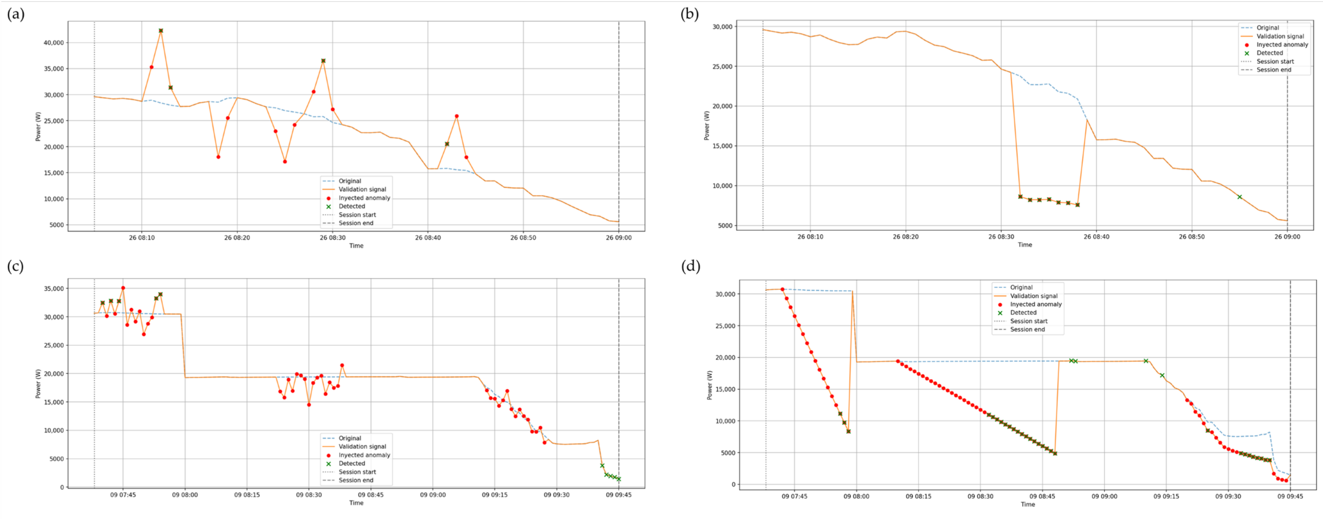
Figure 3 provides a representative example of the charging consumption anomaly detection task. The visual comparison between the original signal, the signal after synthetic anomaly injection and the model detections illustrates the heterogeneous behaviour observed in Table 3. Abrupt deviations and physically inconsistent perturbations are more clearly identified, whereas progressive or unstable patterns may only be partially detected.

4.2. Non-Charging Consumption Anomaly Detection Results

Table 4 presents the results for consumption anomalies during non-charging operation. In this case, the models performed well when the injected anomaly generated abnormal power levels during periods in which the charger should remain close to standby operation.

Isolation Forest achieved strong performance for residual consumption and unregistered charging events, with high F1-score, PR-AUC and Recall-any values. These anomalies were clearly distinguishable from normal non-charging behaviour. Standby peaks also showed high PR-AUC values, although the point-wise F1-score was lower, indicating that the anomaly score ranked the events correctly, but the operational threshold did not always classify all anomalous samples.

Frozen sensor events were the most difficult non-charging anomaly. Both models obtained very low point-wise performance, indicating that this type of anomaly was not effectively captured using the current point-wise feature representation.

Figure 4 shows a representative non-charging consumption scenario. The example illustrates that abnormal power levels during standby periods can be clearly detected when they produce a visible departure from the normal non-charging baseline. In contrast, anomalies such as frozen sensor values are less evident in a point-wise representation, which is consistent with the lower quantitative performance reported in Table 4.

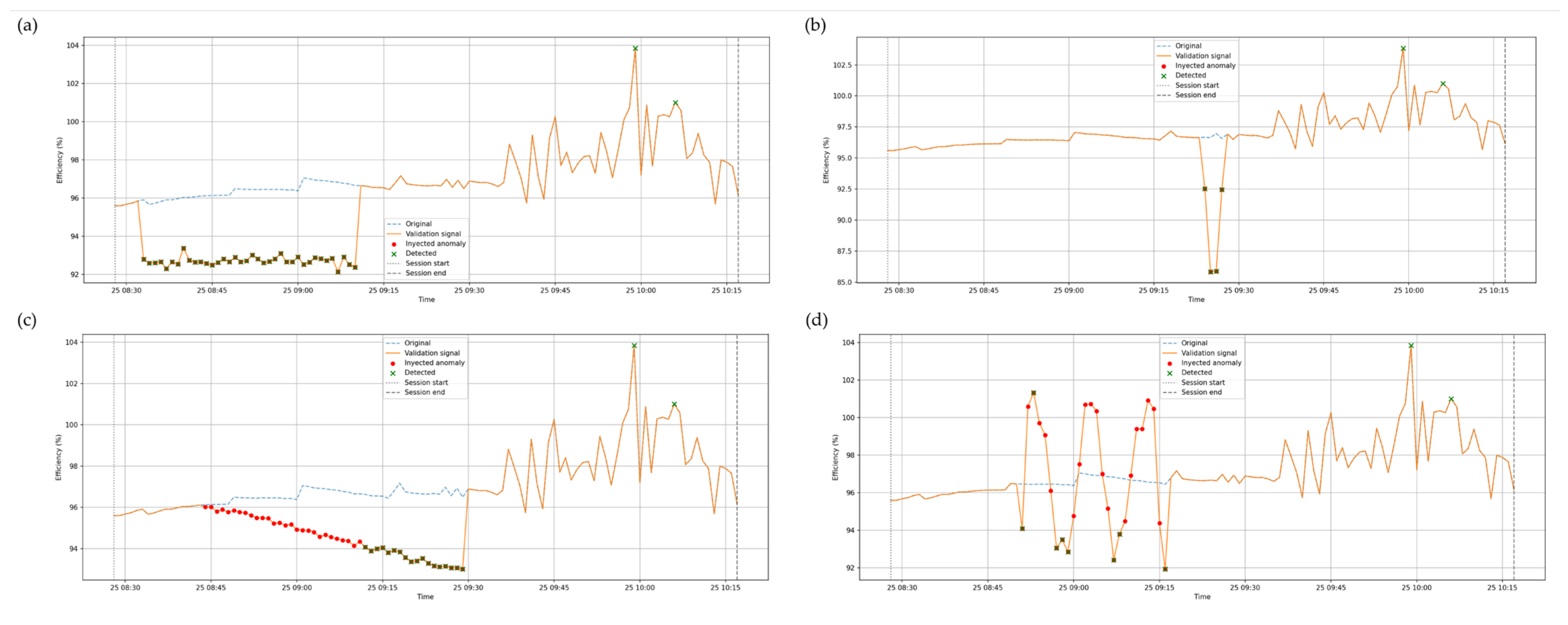
4.3. Efficiency Deviation Detection Results

Table 5 reports the results for the efficiency deviation detection task. In general, efficiency-related anomalies were detected more reliably than consumption anomalies, especially when the deviation was sustained or physically implausible.

Sustained low-efficiency events achieved consistently high performance for both models, with strong F1-score, PR-AUC and Recall-any values. Physically implausible efficiency values were also detected reliably, particularly by LOF. Progressive efficiency degradation showed intermediate performance, with better results at strong severity than at medium severity.

Punctual efficiency drops and unstable efficiency patterns were more challenging in terms of the point-wise F1-score. However, Recall-any remained high, indicating that the occurrence of these events was generally detected even when not all anomalous samples were correctly labelled.

Figure 5 illustrates the efficiency deviation detection task. The visual example shows how deviations between charger-side and grid-side measurements can generate identifiable departures from the normal efficiency-related signal. This supports the quantitative results in Table 5, where sustained or physically implausible efficiency deviations are detected more reliably than punctual or unstable patterns.

4.4. Phase Imbalance Anomaly Detection Results

Table 6 shows the results obtained for phase imbalance anomaly detection. This task achieved the most consistent performance across anomaly families and severities.

Moderate and severe phase imbalances were detected reliably by both LOF and Isolation Forest. Similar behaviour was observed for partial phase drops and near-total phase loss events, which achieved high F1-score, PR-AUC and Recall-any values. These results indicate that the phase balance indicator provides a highly informative representation for detecting abnormal asymmetries in three-phase operation.

Unstable phase behaviour was more challenging than the other phase-related anomalies, particularly at medium severity. Nevertheless, performance improved for stronger deviations, and Recall-any values remained high, indicating that most injected phase instability events were detected at least partially.

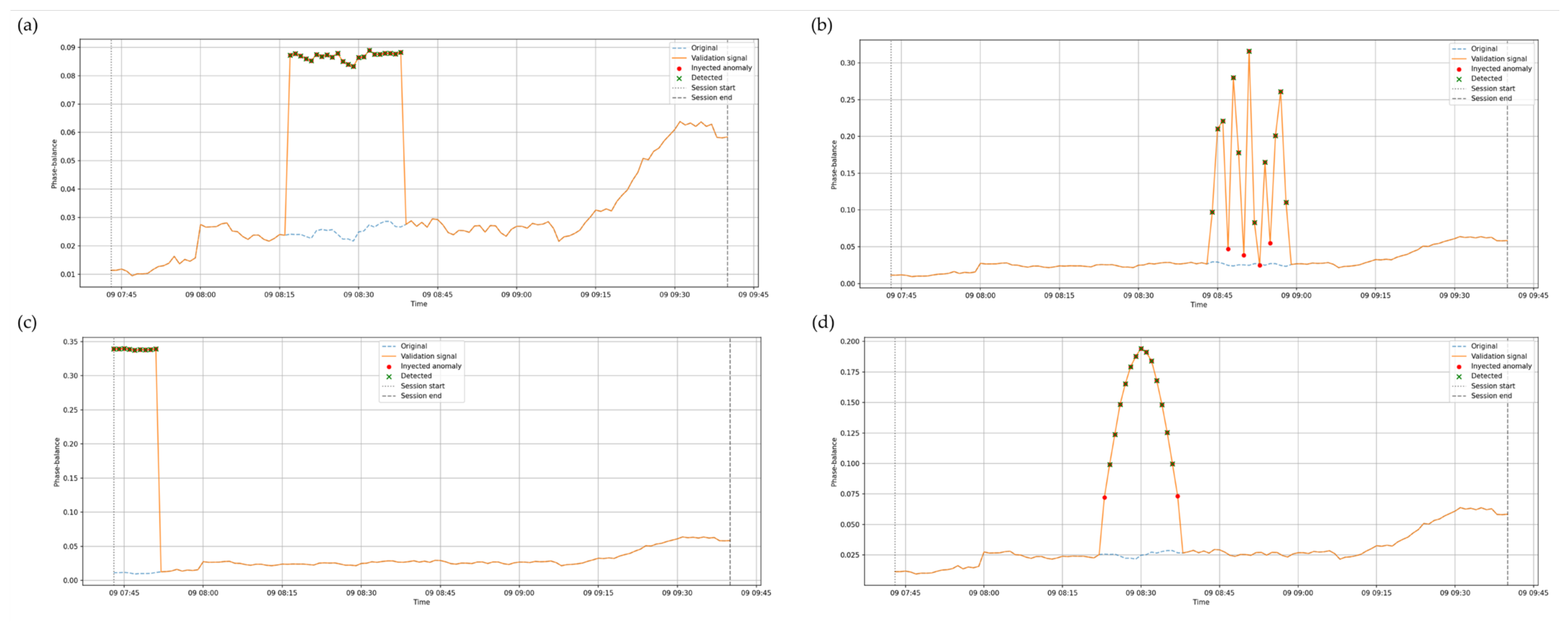
Figure 6 provides a representative example of the phase imbalance anomaly detection task. The injected imbalance produces a clear deviation in the phase balance indicator, which explains the high and consistent performance reported in Table 6. The figure also illustrates the diagnostic value of using a physically informed indicator for this specific monitoring objective.

5. Discussion

The results demonstrate the feasibility of the approach in the monitored DC fast-charging station, while further validation across additional chargers, power levels and operating conditions is required. The strongest performance was obtained for anomalies that generated clear deviations in the feature space, such as sustained efficiency losses, physically implausible efficiency values, phase imbalance, partial phase drops, near-total phase loss, residual consumption and unregistered charging during non-charging operation. These results support the use of unsupervised anomaly detection as an early-warning tool for monitoring DC fast-charging stations.

The three detection tasks provide complementary diagnostic information. Consumption anomaly detection captures global deviations in the electrical behaviour of the charger. Efficiency deviation detection evaluates the consistency between grid-side and charger-side power measurements, which is relevant for identifying abnormal losses, measurement inconsistencies or degraded operating conditions that may affect operating costs and billing accuracy. Phase imbalance detection provides additional information on the symmetry of the three-phase electrical supply, allowing abnormal phase distributions to be detected even when total power consumption may appear normal.

The results also show that model performance depends strongly on the physical nature of the anomaly. Point-wise deviations, sustained abnormal states and physically inconsistent values were easier to detect because they produce samples that are clearly separated from normal operation. In contrast, progressive drifts, unstable behaviours and frozen sensor events were more difficult. This limitation is expected because LOF and Isolation Forest were applied to point-wise feature representations and do not explicitly model temporal dependencies. In these cases, each individual sample may remain close to the normal operating region, while the anomaly is mainly expressed through the evolution of the signal over time.

No single model consistently outperformed the other across all tasks. LOF tended to perform well when anomalies produced local deviations in the feature space, as observed in several efficiency and charging consumption scenarios. Isolation Forest showed strong performance for non-charging consumption anomalies that generated clear global deviations from standby behaviour. In the phase imbalance task, both models achieved similar and consistently high performance, suggesting that the phase balance indicator itself is highly informative for this monitoring objective.

The different behaviour of LOF and Isolation Forest can be explained by their anomaly scoring mechanisms. LOF relies on local density contrasts and is therefore sensitive to samples that lie in regions of lower density than their neighbourhood. This can be advantageous for local deviations in multivariate charging behaviour. Isolation Forest, on the other hand, isolates observations through random partitions and may perform better when abnormal samples occupy globally unusual regions of the feature space, which occurred for several non-charging consumption anomalies. The similar performance of both models in the phase imbalance task suggests that, in that case, the discriminative power came mainly from the physically informed phase balance indicator rather than from the specific anomaly detection algorithm.

An important aspect of the results is the difference between PR-AUC and F1-score. In some scenarios, high PR-AUC values were obtained together with moderate or low F1-scores. This indicates that the anomaly scores were able to rank injected anomalies above normal samples, but the operational threshold derived from the unsupervised model configuration was not always optimal for the test distribution. Therefore, PR-AUC should be interpreted as the intrinsic ranking capability of the anomaly score, whereas F1-score represents the performance obtained with the current thresholding strategy.

From an operational perspective, the proposed framework should be interpreted as a condition monitoring and early-warning tool rather than as a complete prognostic maintenance system. The models identify abnormal operating periods that may support inspection planning and maintenance prioritisation, but they do not estimate remaining useful life or explicitly forecast future failures. Moreover, exceeding a decision threshold indicates a deviation from the learned normal operating behaviour, but does not by itself identify a specific physical fault. Fault attribution therefore requires corroboration with additional diagnostic information, such as charger alarms, maintenance records or complementary monitored variables.

The main limitation of this study is the absence of labelled real fault data. Although the synthetic anomalies were injected into real operational signals and were designed to represent plausible abnormal behaviours, they may not fully capture the complexity of real failure modes. Real faults may involve interacting electrical, thermal, communication and control effects, as well as irregular temporal patterns that are difficult to reproduce through controlled injection. In this study, only electrical operational variables were available, so thermal measurements, detailed communication logs and internal control variables could not be incorporated into the models or validation procedure. In addition, the efficiency-related indicator may be affected by residual timestamp mismatches between the charger-side and grid-side acquisition systems, particularly during rapid power variations. Therefore, the reported metrics should be interpreted as a controlled evaluation of anomaly detectability, rather than as a direct estimate of performance on all possible real faults. A second limitation is the restricted number of active DC fast-charging sessions available in the monitored period. This mainly affects the characterisation of normal behaviour during active charging, efficiency analysis and phase balance analysis. In contrast, the non-charging operating regime is represented over the complete monitoring period, which provides a broader basis for characterising standby behaviour.

Nevertheless, the validation was performed on a specific 30 kW DC fast-charging station. Therefore, the trained models and operational thresholds should be considered station-specific, and their direct generalisation to other charger models, power levels, manufacturers and operating conditions should not be assumed.

Another limitation is the use of fixed operational thresholds derived from the unsupervised model configuration, rather than thresholds calibrated on an independent validation set.

Future work should focus on several directions. First, the framework should be validated using additional DC fast-charging stations and, when available, real documented fault events, charger alarms and maintenance records. Second, additional monitoring variables, such as temperature measurements, communication logs and internal charger status signals, should be incorporated to better characterise failures involving thermal, communication or control effects. Third, threshold calibration strategies should be evaluated using an independent validation set with synthetic anomaly injection, followed by final assessment on a separate test set. Finally, temporal features or sequence-based models should be incorporated to improve the detection of progressive drifts, unstable behaviours and frozen sensor events. Examples include rolling statistics, first differences, constant-value duration features, change-point detection methods or temporal deep learning models.