Predicting 28-Day Cement Compressive Strength for Delayed Quality Control Using Early-Age Strength and a Weighted CatBoost–XGBoost Ensemble

Abstract

A data-driven and industrially applicable framework was developed to predict the 28-day compressive strength of cement using routine quality control data from the SEZA Cement Plant. Since 28-day strength is obtained only after a substantial delay, the proposed framework was designed to support earlier decision-making during production. To improve predictive capability, 7-day compressive strength was incorporated as an explanatory variable together with plant quality control parameters, thereby linking early-age mechanical response to later-age performance. Before modeling, the dataset was systematically preprocessed through column standardization, numeric type conversion, removal of incomplete observations, and elimination of age-related strength variables other than the target to avoid information leakage. For comparative evaluation, CatBoost, XGBoost, LightGBM, Random Forest, and Extra Trees were implemented. In addition, a hybrid model, termed the ‘Early-Age-Strength-Supported Weighted Dual-Boosting Ensemble’ (EYD-AIBE), was proposed by combining the optimized predictions of CatBoost and XGBoost using fixed weights. Model performance was assessed under both random split and time split schemes in order to evaluate not only overall pattern-learning capacity but also temporal generalizability. Hyperparameter optimization was performed for CatBoost and XGBoost using Optuna. The results showed that EYD-AIBE achieved the best performance in both evaluation settings. Under random split, it yielded R² = 0.535, RMSE = 0.988 MPa, and MAE = 0.785 MPa, whereas under time split, the model achieved R² = 0.405, RMSE = 1.148 MPa, and MAE = 0.900 MPa. These findings indicate that the proposed hybrid framework provides a feasible, reliable, and methodologically robust tool for cement quality control, production monitoring, process optimization, and early decision support.

1. Introduction

As the cornerstone of the infrastructure and superstructure production chain, the cement industry is not only a key driver of construction material production but also a critical determinant of economic sustainability, structural safety, and resource efficiency. Therefore, the accurate, rapid, and reliable monitoring of quality indicators defining the performance of cement and cement-based binding systems during the production process is of great importance not only for verifying the quality of the final product but also for ensuring process stability, optimizing energy consumption, rationalizing raw material usage, and suppressing quality deviations at an early stage. In industrial applications, the 28-day compressive strength stands out as one of the most widely accepted indicators of final performance; it plays a central role in verifying design strength, evaluating batch acceptance criteria, and implementing quality assurance mechanisms. However, the inherently delayed nature of this indicator means results can only be finalized after a 28-day waiting period, creating a significant decision-making challenge for facilities engaged in continuous production. Considering that production continues over days and weeks under varying raw material properties, process conditions, and environmental influences, delayed validation data limits operators’ ability to take corrective actions on the same day or within the same production window, which can lead to outcomes such as quality risks, rework costs, resource loss, and process inefficiency.

From the perspectives of data science and process engineering, this problem is a typical “lagged target variable” problem. In other words, while a large amount of process and quality control data can be measured at the time of production, the primary performance output of interest, 28-day compressive strength, can only be observed with a time lag. Therefore, reliably predicting the 28-day strength using quality control parameters routinely measured at the facility, product characterization data, and early-age test results constitutes a research area of high scientific and industrial value. Such a prediction framework can function like a “soft sensor” that effectively shortens the laboratory feedback cycle; thus, it can generate early warnings regarding quality even before the final test results are available and provide decision support for process optimization.

In recent years, machine learning (ML)-based approaches have rapidly gained traction in the field of cement and concrete materials science. In particular, systematic reviews and comparative studies clearly highlight that machine learning offers greater modeling flexibility compared with classical empirical relationships and simple parametric regressions, especially in problems involving multiple variables, strong interactions, and often nonlinear behavior, such as strength prediction [1,2]. However, the same literature indicates that performance reports often focus solely on accuracy scores; more critical engineering dimensions such as data quality, sample representativeness, validation design, time dependency, and model generalizability are not sufficiently addressed in most studies [1,2]. This is particularly important for industrial applications that work with field data because, unlike controlled datasets obtained under laboratory conditions, plant data contain structural issues such as measurement noise, sampling variability, missing observations, process regime changes, and time-dependent distribution shifts.

Early approaches in the field of strength prediction were primarily based on empirical equations or classical regression-based models developed using a limited number of variables. However, strength development in cement-based systems is a process too complex to be reduced to a single determinant. Numerous factors such as the water-to-binder ratio, binder phase composition, fine aggregate characteristics, admixture type and dosage, grinding fineness, particle size distribution, mineralogical structure, hydration kinetics, porosity development, and curing conditions interact with one another to determine the final strength. Consequently, linear, one-dimensional, or approaches based on a limited variable space often prove insufficient in capturing these complex material process relationships. With the rise in data-driven modeling techniques, artificial neural networks, support vector machines, random forests, and particularly tree-based ensemble learners have begun to offer more powerful alternatives for such problems [1,2]. The recent literature reports that gradient boosting-based ensemble methods have demonstrated remarkable performance on concrete and cement data [3,4,5,6]. This trend is no coincidence; the boosting approach provides high representational power in complex, nonlinear data structures with intense interactions between variables by sequentially improving weak learners. XGBoost has become a powerful reference model in numerous engineering applications thanks to its regularized gradient boosting architecture, flexibility in loss function optimization, and success in capturing nonlinear relationships [7,8]. LightGBM offers significant advantages in terms of training efficiency and computational cost thanks to its histogram-based splitting mechanism and leaf-centric tree-growing strategy [9]. CatBoost, on the other hand, stands out as a more balanced and relatively robust alternative against overfitting, particularly due to its ordered boosting approach and design aimed at reducing prediction bias [10]. Recent comparative studies on concrete strength prediction demonstrate that methods such as CatBoost, XGBoost, and LightGBM frequently rank among the top performers across various data regimes and produce notable results in terms of accuracy–stability balance [3,4,5,6].

Taken together, the cement-process machine-learning studies cited here do not function merely as isolated application examples; they define the technical pathway of the present study. Prediction of clinker phases from plant-scale process variables [11] and online f-CaO estimation [12] show that latent quality states related to mineralogy and chemistry can be inferred before late laboratory confirmation. Hybrid kiln models [13], SHAP-supported energy models for vertical roller mills [14], electricity-cost optimization frameworks [15], and LSTM-based grinding-energy forecasts [16] further demonstrate that cement production data contain nonlinear, lagged, and time-dependent relationships. These characteristics are directly aligned with the 28-day strength prediction problem, because the target variable is delayed while the explanatory variables are available during or shortly after production. Therefore, these studies motivate the present framework by showing that plant-scale chemical, physical, and early-age mechanical indicators can be converted into an early soft-sensor for delayed quality control.

However, one of the key characteristics that distinguishes real-world plant data from laboratory datasets is that the data generation process exhibits a time-dependent and non-stationary nature. Numerous factors such as changes in raw material sources, fluctuations in clinker chemistry, updates to additive ratios, equipment wear, maintenance activities, operator interventions, revisions to target quality windows, and environmental effects can cause the relationship between input variables and target strength to drift over time. This phenomenon, defined in the literature as concept drift, is recognized as one of the primary causes of performance degradation in deployed machine learning systems [17]. Recent studies on drift detection, retraining timing, window-based update strategies, and the selection of monitoring metrics clearly demonstrate that reliability in industrial ML systems cannot be guaranteed solely by the high accuracy values obtained at the outset [18]. Therefore, high performance scores obtained through random data splitting may present the model’s future success in real-world applications as more optimistic than it actually is. In contrast, validation protocols that preserve temporal order offer a more realistic and engineering-focused evaluation framework by testing how well the model can generalize from the past to the future.

The starting point of this study is precisely this industrial need. Within the scope of the study, a data-driven prediction framework targeting 28-day compressive strength was developed, utilizing both quality control parameters routinely recorded at the plant and early-age compressive strength data. In particular, the inclusion of 7-day strength data in the model is important for leveraging the continuity between early-age mechanical response and the development of ultimate strength, because early-age strength often provides a strong summary of hydration level, binder reactivity, and initial microstructure development. However, 7-day strength alone is insufficient; when considered alongside process and product characteristics, predictive power increases significantly. Therefore, the study is built on a multivariate and interactive prediction framework rather than a single correlation. To ensure data integrity and training–test consistency in the modeling process, missing observations were filtered at the row level, and only a training set consisting of complete observations was used. This approach aims to prevent additional uncertainties arising from the differing assumptions of missing data imputation strategies from obscuring model comparisons. In other words, the focus of this study is not on the performance of missing data imputation, but on establishing a consistent and directly comparable prediction pipeline. Within this framework, the proposed hybrid approach is named Early-Age-Strength-Supported Weighted Dual-Boosting Ensemble (EYD-AIBE). The EYD-AIBE architecture is based on the linear combination of two powerful boosting-based learners, CatBoost and XGBoost, trained independently on the same feature space, with fixed weights during the testing phase. The hybrid prediction output is defined as follows [18,19]:

$${\widehat{y}}_{28}=0.80 {\widehat{y}}_{CatBoost}+0.20 {\widehat{y}}_{XGBoost}$$

(1)

Here, ${\widehat{y}}_{28}$ represents the predicted 28-day compressive strength, while ${\widehat{y}}_{CatBoost}$ and $y_{XGBoost}$ denote the predictions of the respective base learners. The primary motivation behind this approach is to obtain a more balanced final prediction by leveraging the fact that the errors produced by the two models on the same data are not entirely identical. By combining CatBoost’s more consistent and relatively stable prediction behavior with XGBoost’s ability to capture complex nonlinear patterns, the goal is to balance the bias and variance issues that could arise from relying on a single learner. Thus, the method produces an ensemble effect while maintaining the advantages of interpretability, ease of maintenance, and deployment simplicity without requiring the more complex second-layer structures typical of stacking [18,19].

Another important aspect of the study is that the model evaluation design is not solely focused on generating high scores, but is also structured to reflect real-world usage conditions. To this end, the Early-Age-Strength-Supported Weighted Dual-Boosting Ensemble (EYD-AIBE) approach and the individual models under comparison were tested under both random data splitting and the time-split protocol, which preserves the temporal order. While random splitting is useful for demonstrating the extent to which the model has learned general patterns in the data space, it presents a test scenario where past and future data are intermixed, which may yield relatively optimistic results for field deployment. In contrast, the time-split evaluation represents a more realistic scenario where the model is trained solely on past observations and applied to future production periods. Therefore, the combined use of these two evaluation approaches allows for a discussion not only of nominal accuracy but also of temporal generalizability and operational reliability [18,19,20].

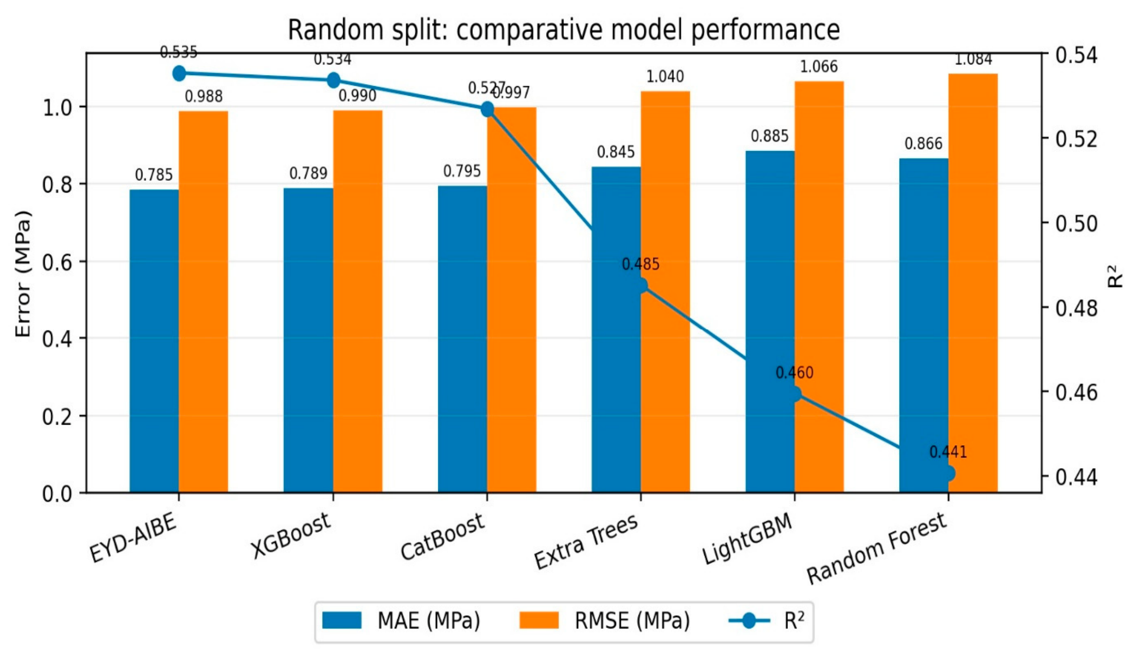
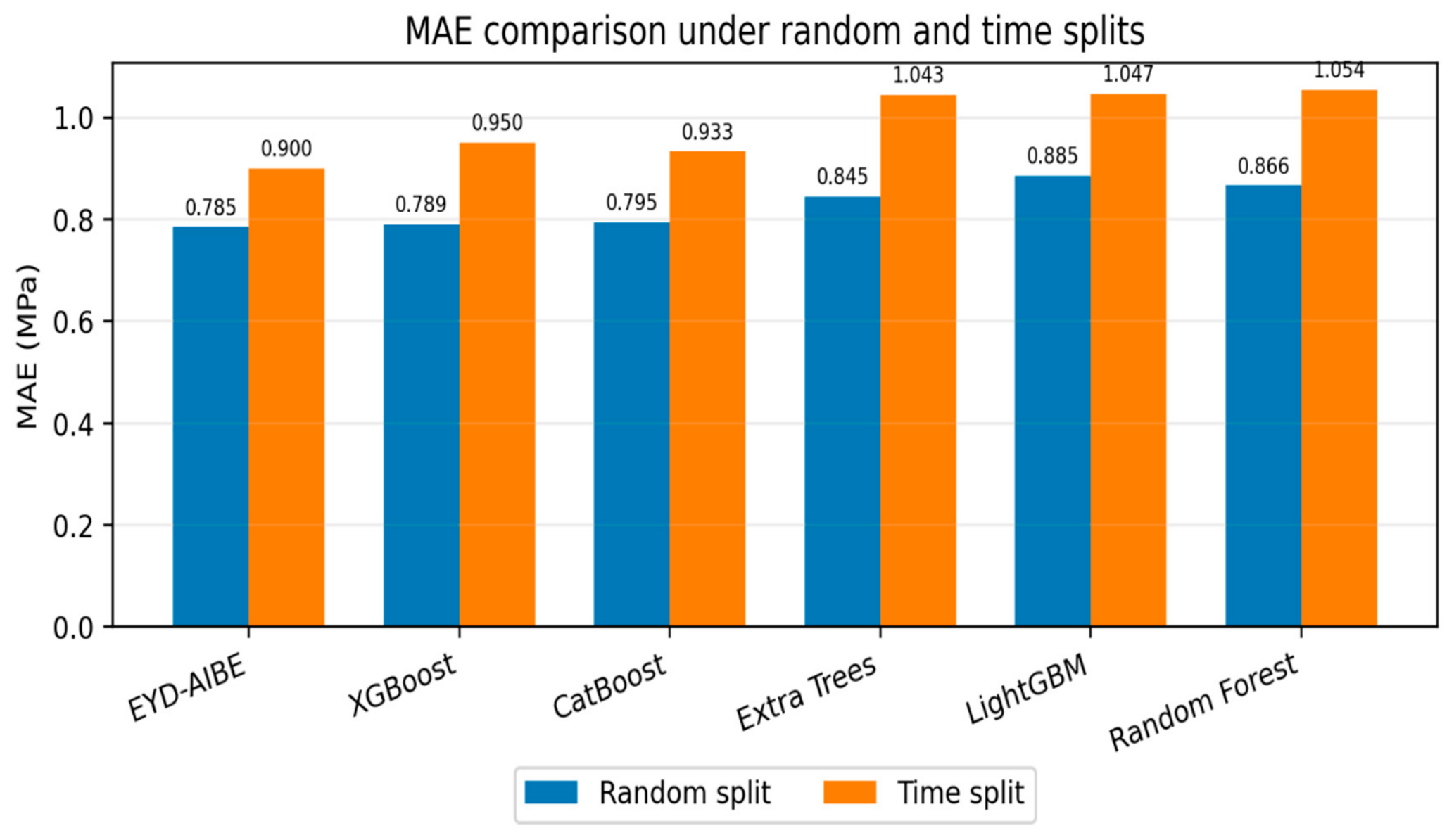
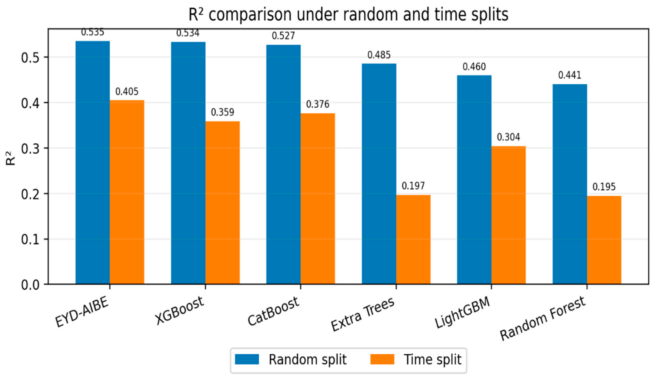
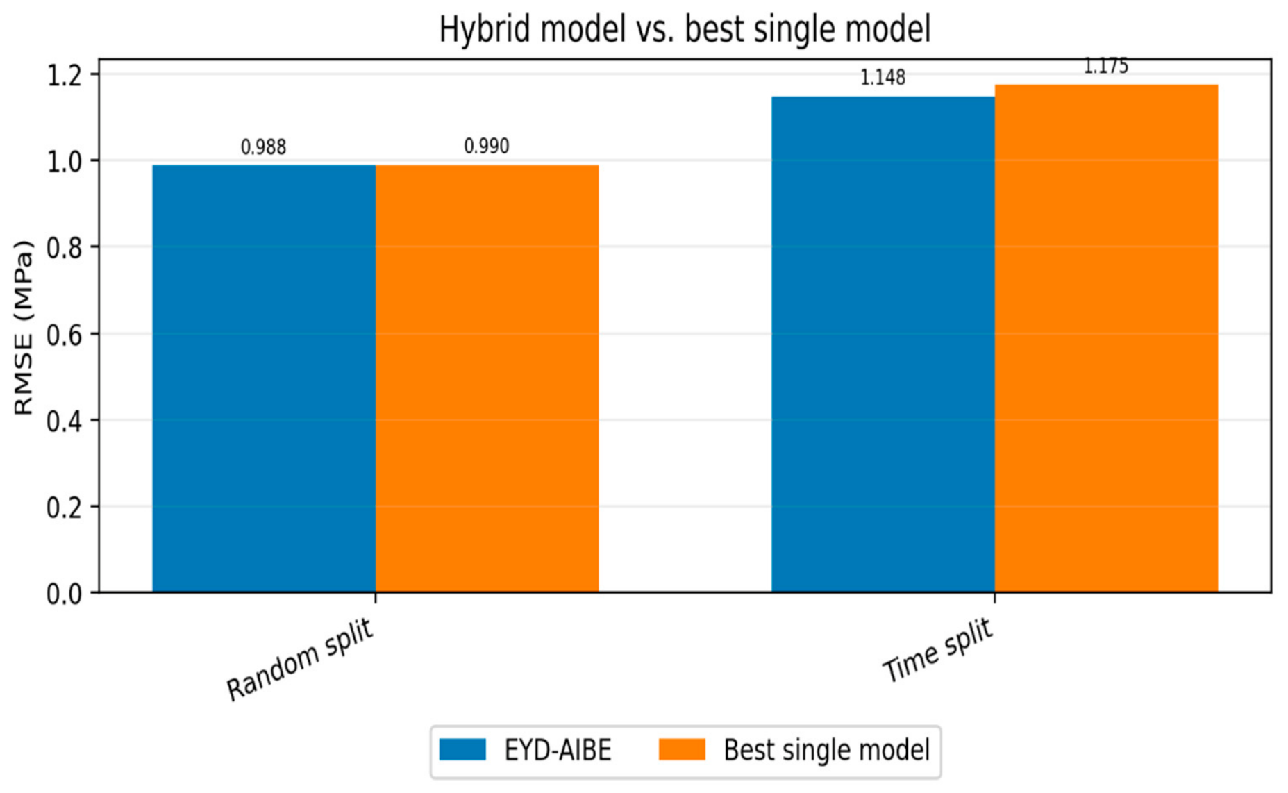
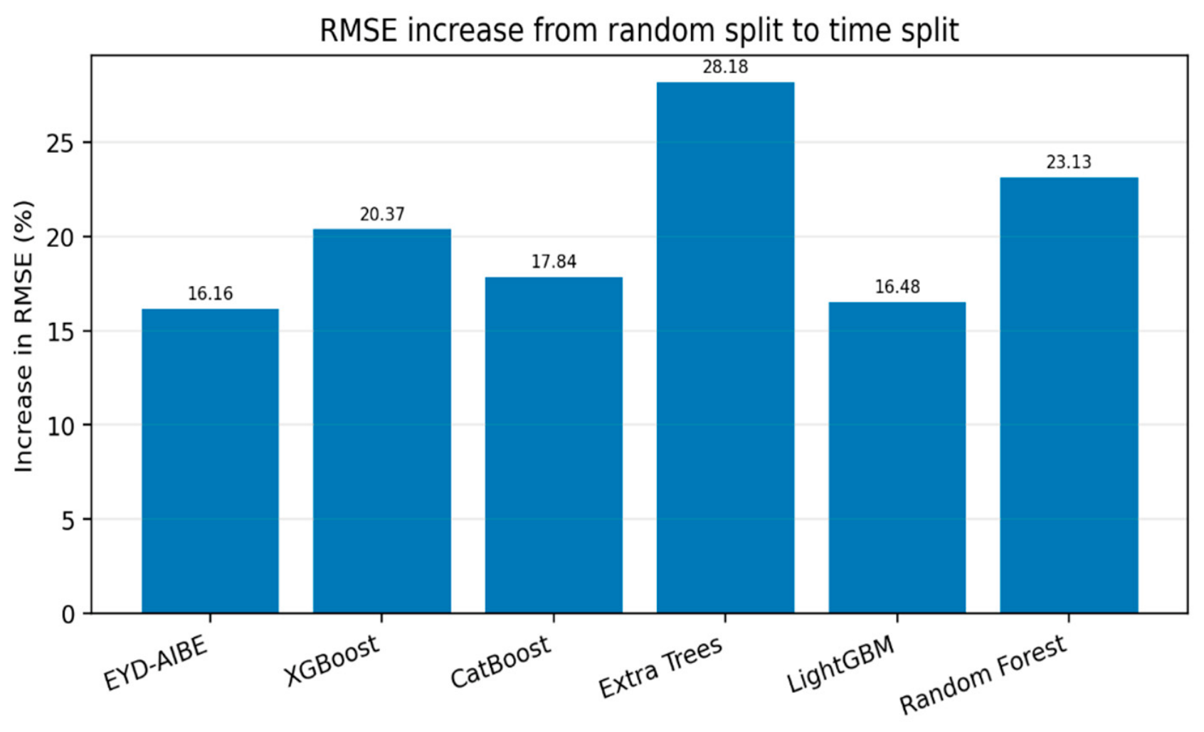
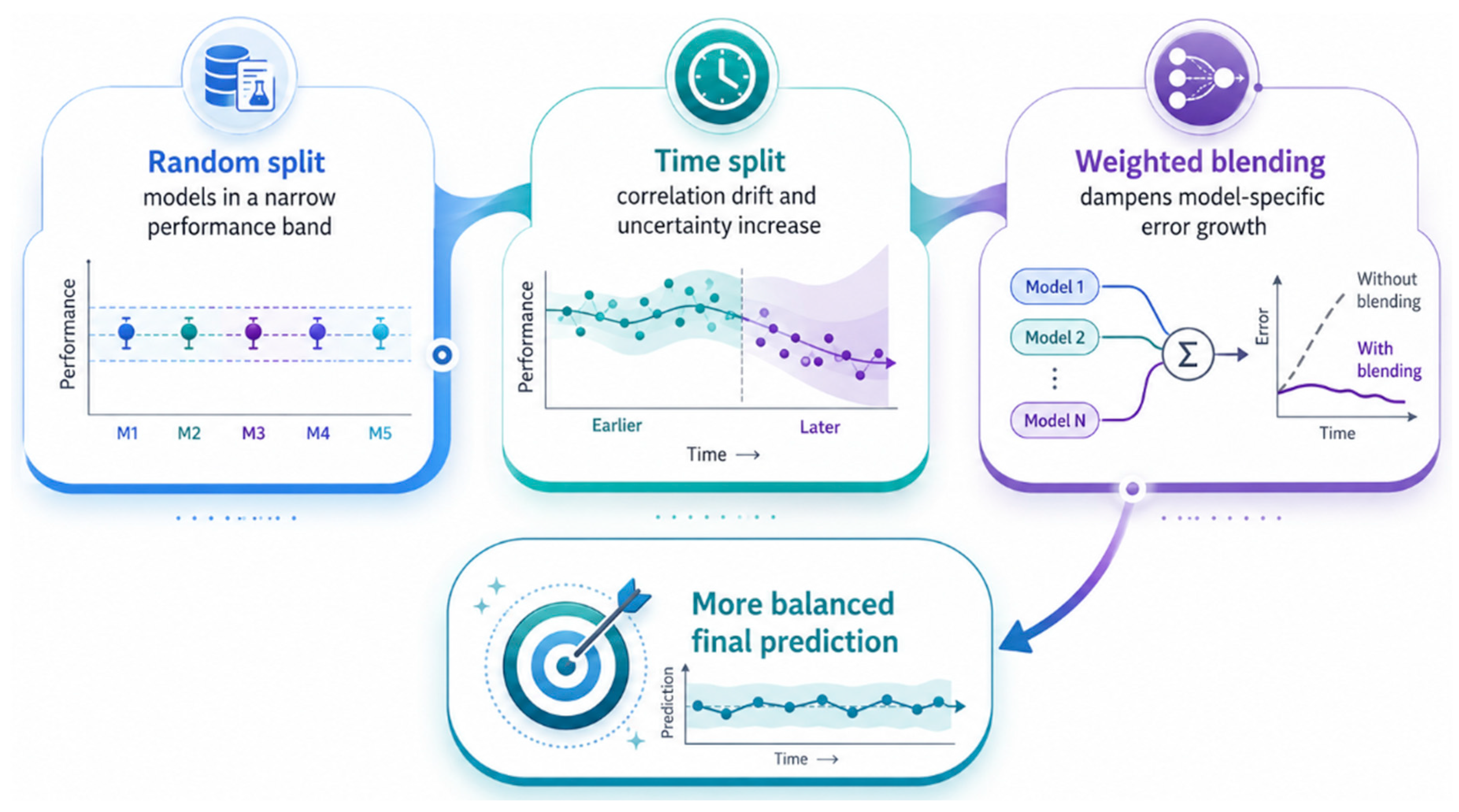
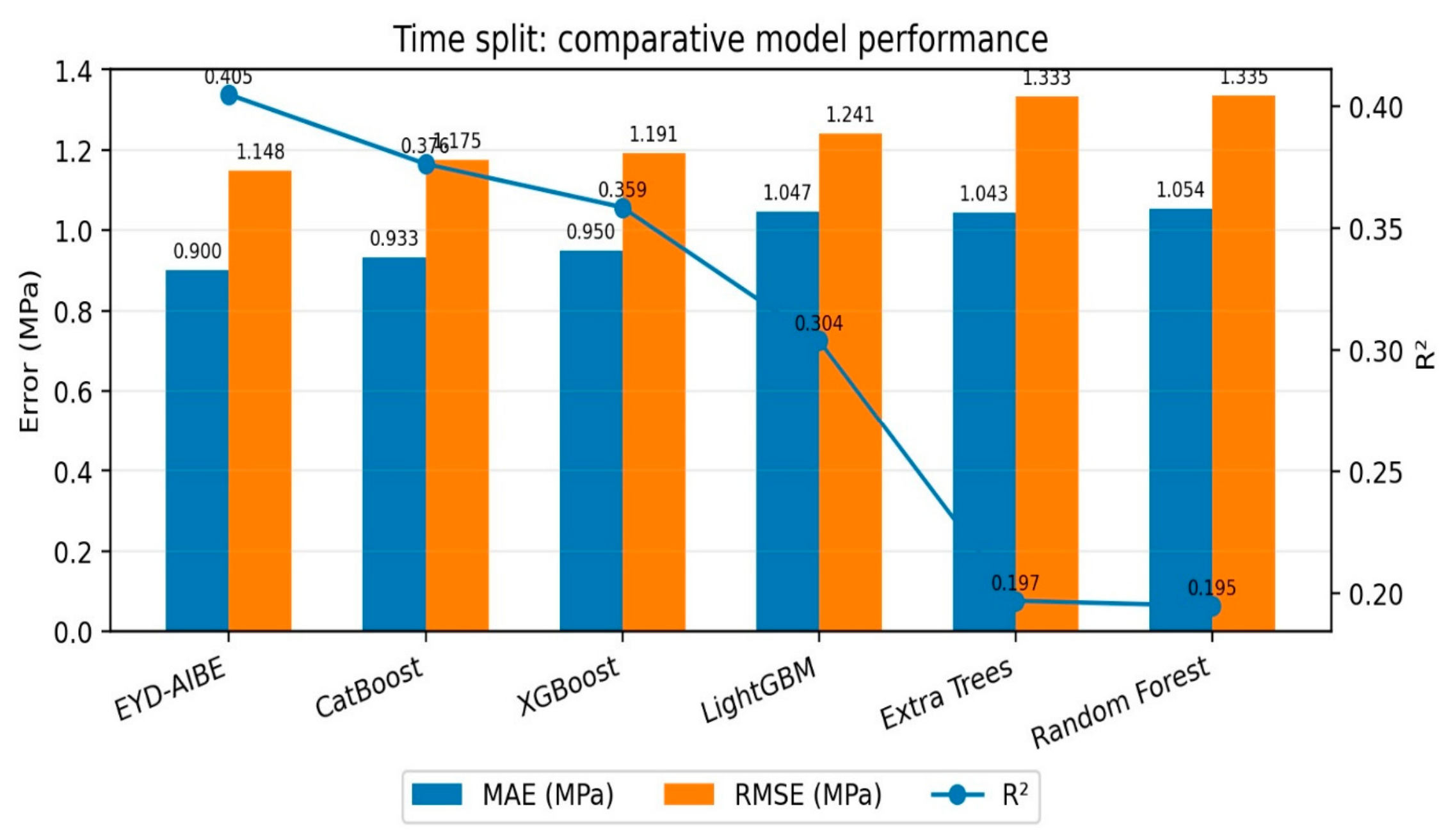
The results show that the Early-Age-Strength-Supported Weighted Dual-Boosting Ensemble (EYD-AIBE) approach demonstrates competitive forecasting performance in random splitting $(R^2 \approx 0.535, RMSE \approx 0.988, MAE \approx 0.785)$, while in time-based partitioning, despite a general decline in performance, it offers a more balanced and stable behavior compared with individual models $(R^2 \approx 0.405, RMSE \approx 1.148, MAE \approx 0.900)$. This decline observed in the temporal segmentation indicates not so much model failure as the structural complexity of the industrial data production process. In other words, as the composition of raw materials, process settings, and operational strategies change over time, the input–output relationships also shift; consequently, it becomes difficult to directly transfer patterns learned from past data to the future. This finding demonstrates that high accuracy alone is insufficient in industrial quality prediction; the temporal dimension, data drift, and retraining strategies must also be treated as essential components of model design [18,19,20].

In this context, the original contribution of this study can be evaluated along three main axes. First, because the study was developed directly on industrial quality control data, it differs from laboratory-scale idealized datasets and presents a prediction problem that is closer to real-world conditions. Second, the Early-Age-Strength-Supported Weighted Dual-Boosting Ensemble (EYD-AIBE) approach is proposed, which utilizes early-age strength alongside process/product indicators and combines two powerful boosting learners within a fixed-weight, simple ensemble structure. Third, model performance is evaluated not only through random cross-validation but also via time-series evaluation, thereby highlighting the temporal generalization dimension, which is far more critical for industrial deployment. Accordingly, the objective of this study extends beyond model-level performance comparison to include the identification of an evaluation design that best captures real field conditions and an ensemble structure that ensures a practical balance between predictive capability and industrial usability.

In conclusion, this research proposes a machine learning-based, industrially applicable approach centered on temporal generalizability for predicting delayed quality outputs, such as 28-day compressive strength, in the cement industry. In the remainder of the study, the data structure, modeling pipeline, implementation of the Early-Age-Strength-Supported Weighted Dual-Boosting Ensemble (EYD-AIBE) architecture, comparative experiments, and random/temporal validation scenarios will be presented in detail; furthermore, the findings will be discussed from the perspectives of concept drift, model stability, interpretability, and sustainable field deployment.

2. Theoretical Background and Conceptual Framework

This section links the material mechanism of strength development with the data-driven modeling logic used in the study. Instead of repeating general algorithmic descriptions, the discussion is organized around three compact issues: the physical meaning of early-age strength, the structure of facility-scale chemical and physical indicators, and the need for validation schemes that reflect delayed industrial quality control.

The physical basis for the development of compressive strength lies in the reaction of cement particles with water, which over time forms a load-bearing binder network. Throughout the hydration process, the formation of calcium silicate hydrate (C–S–H) gel, the refinement of the pore structure, the reduction in capillary porosity, and the strengthening of interparticle bonding are the primary determinants of mechanical strength gain. This process is not a single-step reaction but a multi-stage, time-dependent transformation mechanism; dissolution and nucleation in the early stages, accelerated hydration formation in subsequent stages, and a diffusion-controlled, slowing reaction regime later on all play a role in the development of the final microstructure. Therefore, 28-day strength is not merely an independent outcome measured at a late age, but the cumulative result of early-age reactions, binder phase transformations, and microstructural consolidation [21]. For this reason, any theoretical framework aimed at understanding strength development must consider both the chemical–microstructural nature of hydration and how this structure translates into a mechanical response. From this perspective, estimating 28-day strength using plant quality control measurements and early-age performance indicators cannot be viewed merely as a statistical prediction problem. Such an approach also serves as a decision-support mechanism that provides early warnings for the production process, makes quality risks visible in advance, and enables timely adjustments to process parameters. In particular, the strong correlation between early-age indicators—such as 7-day compressive strength and 28-day performance is consistent with the fundamental physics of material behavior. This is because the early-age strength value consolidates the combined effects of numerous parameters such as cement composition, grinding fineness, hydration rate, mineral-additive interactions, water-to-binder ratio, and initial microstructural development into a single measurable performance signal. In other words, the early-age strength measurement represents the net mechanical outcome of these transformations under field conditions, even if all microstructural transformations are not directly observed [22]. This characteristic makes it possible to evaluate 7-day strength not merely as an auxiliary variable, but as a robust intermediate indicator that constrains the path to ultimate strength and lends physical meaning to the model.

However, in cement-based systems, strength development is not merely a linear extension of the early-age mechanical response. Ultimate strength is shaped by the interaction of numerous variables, including clinker phase distribution, alite and belite reactivity, gypsum balance, type and proportion of mineral admixtures, particle size distribution, specific surface area, mix homogeneity, curing temperature, humidity conditions, and even differences in specimen preparation. Therefore, reliably predicting 28-day strength requires modeling approaches capable of capturing multivariate and nonlinear relationships. While classical linear regression frameworks can be useful in certain scenarios, they are often limited when dealing with high-order interactions between variables, threshold behaviors, and process-induced heterogeneities. This is the fundamental reason behind the growing prevalence of data-driven methods: machine learning approaches can represent complex input–output relationships more flexibly and integrate multiple quality/process indicators within the same modeling space.

The rapid expansion of machine learning applications in the concrete and cement sector in recent years has demonstrated that problems such as strength prediction cannot be adequately explained by experimental correlations alone. Studies using techniques such as tree-based ensemble methods, boosting approaches, support vector machines, and artificial neural networks have demonstrated that higher accuracies can be achieved compared with classical approaches in nonlinear and multivariate structures. However, a crucial theoretical point is that high performance scores alone do not guarantee model reliability. Data quality, sample representativeness, missing observation patterns, measurement uncertainty, validation protocols, and the model’s ability to generalize across different time scales are the primary factors determining the engineering relevance of the results [1]. Accordingly, in machine-learning-based strength prediction studies, theoretical rigor requires that model performance be interpreted not only in terms of comparative R² values, but also with respect to the data regime, validation design, and generalizability limits that define the conditions under which such performance is obtained.

This situation is even more pronounced for models that work with facility data. Industrial quality control datasets often contain small or medium-sized sample sizes; at the same time, they harbor multi-layered sources of uncertainty such as measurement noise, missing values, sampling variations, changing operational strategies, and time-dependent distribution shifts. In low-data regimes, the risk of the model overfitting the training data increases, while performance evaluation may also become overly sensitive to the data partitioning strategy used. Therefore, one of the most critical theoretical issues under low-data conditions is striking the right balance between model complexity and generalizability. While an overly flexible model may learn the noise in the training data, an overly simple model may fail to adequately represent the true nonlinear structure between material and process. This dilemma elevates validation design, particularly in industrial applications, from a mere technical detail to a fundamental element determining the scientific reliability of the method [23].

The second critical aspect here is that the data exhibits a non-stationary structure over time. The relationship between input variables and 28-day strength may change over time due to factors such as changes in raw material sources at cement plants, fluctuations in clinker mineralogy, the operating regime of the grinding circuit, updates to the additive composition, equipment wear, or new operating conditions following maintenance. This situation is addressed in the data science literature under the terms “distribution drift” or, more specifically, “concept drift”. Theoretically, this phenomenon suggests that the relationship learned from past data may not remain constant in the future, and therefore, model validation based solely on random data splits may overestimate actual performance in the field. In contrast, time-series validation strategies provide a more realistic evaluation framework for testing how well the model, having learned from past production periods, can be generalized to future periods. Therefore, the strength prediction problem should be viewed not merely as a matter of modeling material behavior, but as an industrial learning problem that requires testing temporal generalizability.

In this context, the theoretical background has two complementary axes. The first axis is the materials science perspective, which explains the physical relationship between hydration-based microstructural development and early-age performance indicators and the ultimate compressive strength. The second axis is the data science perspective, which discusses how this physical relationship can be learned from real plant data, which validation strategies should be used to test it, and under what conditions model reliability should be interpreted. These two axes are not independent but directly interrelated: a model that is physically nonsensical cannot produce sustainable decision support even if it yields high accuracy; conversely, a model that is statistically weak or over-optimized, even if grounded in physical intuition, may not be reliable in field applications. Therefore, a robust methodological framework for predicting 28-day strength in the cement industry must integrate both the material-based causal structure and the generalizability principles of data-driven learning.

2.1. The Relationship Between Hydration and Strength and the Importance of Early-Age Indicators

The development of compressive strength in cement-based systems relies on the clinker phases reacting with water over time to form a load-bearing, interconnected, and progressively densifying binder microstructure. During this process, the formation of calcium silicate hydrate (C–S–H) gel, along with the development of calcium hydroxide and aluminate/ferrite-based hydrate phases, increases intergranular bonding strength; capillary pore volume and pore continuity decrease; consequently, the material’s permeability decreases, and a more stable internal skeleton forms under mechanical load. Therefore, the increase in strength cannot be explained solely by an increase in the degree of hydration; it is also directly related to the spatial distribution of reaction products, the efficiency of pore filling, the disruption of the capillary pore network, the strengthening of intergranular contact zones, and the relative suppression of defect density in the microstructure. In other words, hydration is more than a chemical transformation; it is a microstructural reorganization process that determines mechanical behavior [21].

The time-dependent nature of hydration also explains why strength development is not linear. In the early stages of the reaction, dissolution, nucleation, and accelerated hydration formation make the mechanical gain more pronounced, whereas in later stages, the rate of strength increase gradually decreases due to a diffusion-controlled and relatively slower reaction regime. Therefore, compressive strength should not be considered a direct function of a single material parameter; rather, it should be evaluated as a multivariate output determined by the combined influence of cement composition, clinker mineralogy, grinding fineness, specific surface area, sulfate balance, type and proportion of mineral admixtures, water requirement, curing conditions, and production-related heterogeneities. This multi-component nature of strength is particularly important for models that utilize field data; because even under seemingly similar production conditions, the microstructural development pathway can vary, which can result in significant differences in the final 28-day strength [21].

In this context, early-age strength, particularly 7-day compressive strength, serves as a strong intermediate indicator representing the development path leading to 28-day performance. The fundamental reason for this is that early-age strength is not merely a standalone test result; rather, it summarizes the combined effect of the cement’s initial reactivity, fine material characteristics, hydration kinetics, additive–sulfate balance, mixture homogeneity, and initial microstructural consolidation into a single measurable performance parameter. Therefore, early-age strength can be considered the “net mechanical output” of numerous intermediate mechanisms that are difficult to observe directly. In other words, even though the model does not measure all microstructural transformations individually, the 7-day strength carries the combined result of these transformations under actual field conditions, thereby generating high predictive value for the 28-day prediction problem [22].

Another reason why early-age strength is such a strong predictor is that the path to ultimate strength does not follow a completely free-running development. If low reactivity, insufficient fineness, an inappropriate sulfate balance, or additive-induced kinetic delays are observed in the early stages, these effects typically limit late-age strength to some extent; similarly, rapid and balanced microstructure formation in the early stages usually provides a favorable foundation for higher 28-day strength. Of course, 7-day strength alone does not deterministically define the 28-day value; late-stage hydration additives, long-term curing conditions, and late reaction mechanisms specific to certain binder systems can alter the final outcome. Nevertheless, early-age strength significantly narrows the uncertainty space, enabling the model to learn more robust and physically consistent relationships [22].

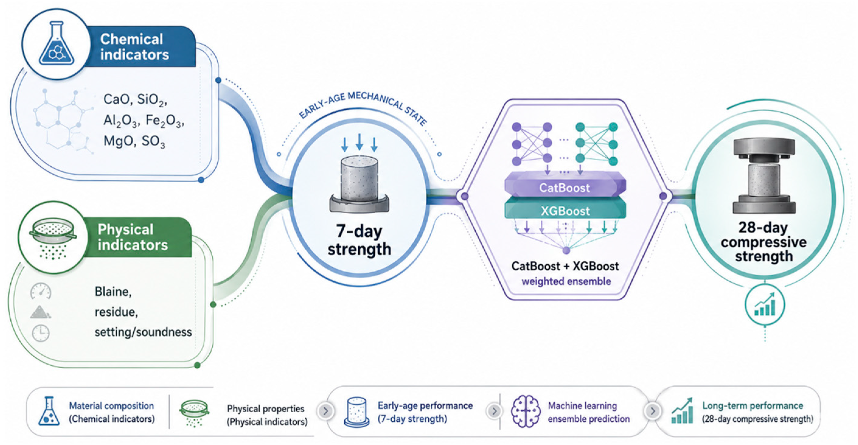
This situation becomes even more critical at the plant scale. Fluctuations in raw material sources, changes in grinding efficiency, updates to process settings, minor deviations in additive dosages, and day-to-day variations in operational conditions can simultaneously alter several mechanisms governing final strength. Monitoring each of these effects individually and in real time is often impractical. In contrast, early-age strength serves as an intermediate output that can be measured, standardized, and incorporated into production-line decision support despite this multidimensional variability. In this regard, 7-day strength is not merely a quality-control variable describing prior performance; it also functions as a bridge variable with high information density, strong physical relevance, and considerable industrial applicability for predicting 28-day compressive strength. As conceptually illustrated in Figure 1, the inclusion of early-age indicators establishes a direct link between cement chemistry, physical fineness characteristics, early mechanical response, and delayed 28-day strength. Therefore, incorporating early-age indicators into the model constitutes a fundamental methodological choice that both improves predictive accuracy and strengthens the model’s consistency with material behavior [22].

2.2. Facility-Scale Data Space and Learning Difficulty

In the present modeling space, the chemical indicators were treated as oxide and modulus descriptors, including CaO, SiO₂, Al₂O₃, Fe₂O₃, MgO, SO₃, loss on ignition where available, and derived cement chemistry modules such as LSF, SM, and AM. The physical indicators comprised Blaine fineness, sieve residue fractions, specific gravity or density, setting-time indicators, soundness, water demand/standard consistency when recorded, and the 7-day compressive strength used as an early-age mechanical state variable. These variables were selected because they jointly represent clinker chemistry, grinding quality, sulfate balance, physical fineness, and early hydration response, all of which are directly related to late-age strength development.

These variables do not typically affect the 28-day compressive strength through independent and linear contributions; rather, they exert influence through threshold behaviors, mutual interactions, contextual sensitivity, and hidden intermediate mechanisms. Even within the same nominal chemical composition range, the final strength response can vary significantly when grinding efficiency, particle size distribution, mineralogical phase equilibrium, additive interactions, hydration kinetics, and mixture homogeneity differ. Therefore, the relationship observed in the data space corresponds to a heterogeneous pattern where different sensitivities dominate in different subregions, rather than a simple structure that can be explained by a single global trend. In other words, the effect of a specific variable on strength may not be constant across the entire dataset; while the same variable may have a pronounced effect in one subregion, it may only become meaningful in another region through interactions with other variables. This context-dependent sensitivity is one of the key factors explaining why models based on a single average relationship are limited, particularly in industrial data.

Another distinctive feature of the plant-scale data space is the intertwining of observable parameters with unobservable process mechanisms. The oxide percentages, fineness values, or physical test results recorded in the quality control system are often merely indirect reflections of the fundamental microstructural processes affecting strength. Certain determinants such as reactivity differences, particle shape, amorphous phase content, microstructural packing efficiency, or the spatial distribution of hydration products may not be directly present in the routine quality control database; nevertheless, they continue to influence the final strength. This situation transforms the modeling problem not only into a multivariate problem but also into a learning problem involving partially latent mechanisms. Consequently, the model’s success depends not only on the number of variables in the dataset but also on the extent to which the available variables can represent the underlying physical processes. The literature particularly emphasizes that while data-driven models can yield robust results in such industrial problems, for these results to be considered reliable, the data preparation steps, including missing value policies, handling of outliers, feature selection, the rationale for using derived variables, and potential data leakage risks, must be presented in a transparent and well-justified manner [1].

The limited number of samples in material and process data is one of the key factors that further exacerbates learning difficulties. In small- or medium-scale datasets, the model may tend to learn random fluctuations and noise specific to the training data rather than the true structure underlying the variables. This situation increases the risk of overfitting and can cause performance that appears high in the training set to deteriorate rapidly when test conditions deviate even slightly from training conditions. This problem is even more pronounced in industrial data, as the data is not only limited but also heterogeneous, partially noisy, and time-sensitive. In such an environment, while high-capacity models may appear theoretically more powerful, they can produce deceptively optimistic results if regularization is not applied or if the validation protocol is not sufficiently rigorous.

Therefore, the key factor determining model success under small-data conditions is not merely the algorithm used, but the extent to which model complexity can be controlled within the bias–variance trade-off framework. Regularization strategies, the controlled selection of hyperparameters such as early stopping, tree depth, or learning rate, the pruning of unnecessary variables, and a training–test split that does not lead to data leakage become critical for the model’s generalizability. In particular, the significant fluctuations in performance obtained from different random splits on the same dataset clearly demonstrate how sensitive evaluation is in small-data regimes. Therefore, methodological rigor in such data structures often carries greater importance than marginal improvements in model architecture.

In conclusion, predicting 28-day compressive strength on plant-scale quality control data is not merely a multivariate regression problem; it is a challenging learning problem involving collinearity, heterogeneity, latent process effects, limited sample size, measurement uncertainty, and potential temporal variations. Therefore, it is clear that model selection alone is insufficient; the logic of data preparation, the structure of the feature space, regularization principles, and especially the evaluation protocol must be discussed at a theoretical level alongside the methodology [23]. Therefore, in industrial strength prediction, reliable performance should be interpreted as a function not only of model selection, but also of the data regime, methodological constraints, and validation design within which the model is trained and evaluated.

2.3. The Theoretical Basis of Tree-Based Ensemble Models

Ensemble learning is a learning paradigm that aims to reduce the generalization error of a single model by systematically combining the outputs of multiple base learners. The fundamental basis of this approach is that different learners do not represent patterns in the data space in the same way, and therefore their error components do not perfectly overlap. If multiple models exhibit different strengths in different subregions and their error patterns do not show perfect correlation, the total error can be reduced with an appropriate combination strategy. Theoretically, this situation can be interpreted within the context of the bias–variance trade-off: some ensemble structures are particularly effective at reducing variance, while others serve to balance both bias and variance. For this reason, ensemble learning can offer more robust and generalizable prediction behavior compared with individual models, especially in nonlinear, highly interactive, and heterogeneous data structures [24].

Tree-based ensemble models hold particular importance for industrial quality control data within this general framework. The fundamental advantage of decision trees is their ability to learn nonlinear relationships, high-order interactions among variables, and local behavioral differences by partitioning the data space into threshold-based regions, without requiring explicit feature transformations. In other words, tree structures do not rely on the assumption that a variable’s effect remains constant across the entire data space; they can model distinct behaviors below and above a specific threshold value. This feature is particularly well-suited for representing the conditional sensitivities frequently encountered in quality control data from cement plants. For example, while the effect of Blaine fineness on strength becomes pronounced within a specific range of oxide content, it is possible for the same effect to weaken or gain significance in conjunction with a different variable within another range. In such cases, a single global linear model is often insufficient, whereas tree-based approaches can learn different decision rules in different regions of data space. The ensemble structure also enhances generalizability by combining these regional rules in a more balanced and stable manner [24].

Tree-based ensemble methods generally revolve around two main principles: bagging and boosting. In the bagging approach, the goal is to improve prediction stability by training base learners with high variance on different subsamples and averaging their outputs. One of the most common representatives of this class, Random Forest, constructs numerous decision trees on different training subsets created via bootstrap sampling and generates model diversity by using random feature subsets at each node. Thus, the erratic behavior exhibited by individual decision trees in response to small data variations or local noise is suppressed, resulting in a lower-variance, more stable prediction structure [25]. This feature is particularly important in datasets where the number of samples is limited or where measurement errors or field-related noise are present, because while a single decision tree may be overly sensitive to small deviations in the training data, Random Forest balances this sensitivity with the ensemble average.

Another important method within the bagging family is the Extremely Randomized Trees (ExtraTrees) approach. In this method, randomness is used more extensively not only during the sampling phase but also in the selection of split points. In other words, instead of deterministically searching for the best split, a more random selection mechanism is employed among candidate splits. As a result, model diversity increases, correlation among trees decreases, and while similar accuracy levels are maintained in certain data regimes, variance can be further reduced [26]. Bagging-based frameworks such as Random Forest and ExtraTrees are considered robust starting models for industrial tabular data problems, particularly because they exhibit relatively resilient behavior against overfitting while capturing complex variable interactions. However, while these methods are generally robust and stable, they may fail to sufficiently reduce bias in certain problems; particularly when dealing with complex and subtle patterns between the target variable and the inputs, more adaptive learning mechanisms may be required.

This is where the boosting approach comes into play. The fundamental logic of boosting involves constructing learners not independently but sequentially, with each new learner focusing on error regions that were not sufficiently represented in the previous stage. Thus, the model not only produces an average behavior that reduces variance but also works to reduce bias by gradually correcting systematic errors. In gradient boosting-based methods, this process is carried out using successive trees that progress in the direction of the gradient of the loss function. Since each new tree attempts to learn the residuals or error trends of the current model, the overall structure can represent complex nonlinear relationships quite effectively. Considering that in industrial quality control data, many variables are interdependent, partially collinear, and context-sensitive, the boosting approach is theoretically well-suited for capturing this complex relationship structure.

Another key advantage of boosting-based methods is that they offer high representational power on tabular data while possessing clearly controllable regularization mechanisms. Model complexity can be controlled through hyperparameters such as tree depth, learning rate, number of trees, subsampling rate, and column selection strategies. This is particularly critical for small and medium-sized industrial datasets, as a model offering high flexibility also carries the risk of overfitting. Strategies such as regularization and early stopping within the boosting family help mitigate this risk, enabling a more balanced learning process. Consequently, boosting methods constitute a theoretically suitable class for material–process problems such as strength prediction, not only due to their high accuracy potential but also because they allow for the controlled management of complexity.

The theoretical strength of tree-based ensembles stems not only from their ability to learn complex patterns, but also from their ability to collectively represent local behavioral differences within the data space. In industrial datasets, the same combination of input variables can produce different target outcomes across different production regimes; in other words, the data space may consist not of a single homogeneous structure, but of sub-regimes that are partially similar yet distinct. While tree-based models can construct node structures sensitive to these sub-regimes, the ensemble framework aggregates these different local representations to produce a more robust final prediction. Therefore, tree-based ensembles provide a more suitable theoretical foundation for cement quality data where variables such as oxide composition, modules, fineness, and early-age strength are used together compared with individual parametric models [24,25,26].

Another important extension of the ensemble approach in this context is the blending of outputs from different tree-based learners under a second aggregation rule. Theoretically, such blending or stacking structures are based on the assumption that a single model family cannot demonstrate the same performance across all regions of the data space. One model may be stronger in certain subpatterns, while another may be more reliable in different subpatterns. If the error profiles of these models do not fully overlap, combining their outputs with appropriate weights can yield a more stable overall performance. This approach is particularly meaningful in industrial data, as noise, measurement uncertainty, partial heterogeneity, and time-dependent regime shifts in field data can cause different learners to respond differently. Fixed-weight blending strategies allow leveraging this complementarity without constructing more complex meta-learner architectures. Thus, the method remains computationally and maintenance-wise simple while benefiting from the ensemble effect.

In conclusion, the theoretical superiority of tree-based ensemble models can be summarized in three main points: first, their ability to naturally represent nonlinear relationships and variable interactions; second, their ability to balance different components of generalization error through bagging or boosting; and third, their ability to produce more robust predictions by combining the complementary error patterns of different learners. These features make tree-based ensemble approaches a theoretically robust and industrially applicable modeling framework for predicting 28-day compressive strength using multivariate, partially collinear, heterogeneous, and noisy quality control data obtained from cement plants [24,25,26].

2.4. Gradient Boosting and Modern Tree Ensembles

The boosting family is a powerful ensemble paradigm that operates on the principle of sequential learning; by having each new learner focus on the error components that the previous ensemble could not explain, it tends to reduce bias in particular. While bagging-based methods are primarily aimed at reducing variance, the boosting approach aims to establish a more precise functional approximation by gradually improving the regions where the model systematically underrepresents. For this reason, boosting offers distinct advantages in data structures where nonlinearities, threshold behaviors, local interaction patterns, and context-sensitive variable effects are dominant [27]. Cement quality control data thus constitute a natural application area for boosting because oxide composition, modulus values, fineness indices, and early-age performance parameters typically determine the target variable not through independent and linear contributions, but through jointly arising conditional effects. For example, the effect of sulfate balance may become more dominant within a specific fineness range, while in another region, the effect of the same variable may remain limited. The boosting framework provides a suitable structure for progressively learning such complex conditional interactions.

Gradient boosting formalizes this boosting logic through a differentiable loss function. The basic idea is to determine, at each iteration, the direction in which the current model can be most improved according to the loss function, and to add a new weak learner representing that direction to the ensemble. In practice, these weak learners are typically shallow decision trees. Thus, the model is constructed not by learning a complex function in a single step, but as the sum of many small adjustments sensitive to the error structure. The general form of gradient boosting can be expressed as follows [27]:

$$f_M(x)={\displaystyle {\sum }_{m=1}^M}{\rho }_m{h}_m(x)$$

(2)

Here, $h_m\left(x\right)$ denotes the weak learner learned at step m, and ${\mathsf{\rho }}_{\mathrm{m}}$ represents the contribution coefficient of that learner within the ensemble. M represents the total number of learners, and the model’s final output consists of the sum of these incremental components. This structure yields highly successful results in engineering problems, particularly with tabular and heterogeneous datasets, as it effectively represents nonlinear decision boundaries and high-order interactions among variables.

The success of gradient boosting models stems not only from their theoretical flexibility but also from the ability to control their complexity. The learning rate, tree depth, number of iterations, row and column subsampling rates, and regularization terms are the fundamental control mechanisms that determine the model’s bias–variance balance. Using a lower learning rate with a larger number of weak learners can ensure more cautious model updates, thereby reducing the risk of overfitting; conversely, while a higher learning rate and deeper trees may enable faster convergence, they can weaken generalizability. Therefore, although boosting-based methods have high performance potential, selecting appropriate hyperparameter ranges, employing early stopping strategies, and carefully designing the validation process are necessary for this potential to be reliably realized [27]. In short, boosting is not a “magic black box” that produces “high accuracy”; it is a powerful yet delicate learning framework that can easily drift into overfitting on small and medium-sized datasets if not properly regularized.

The modern gradient boosting family includes various implementations that enhance the classical gradient boosting logic in terms of computational efficiency, regularization capability, and generalization power. XGBoost has become a strong reference model for tabular data problems thanks to its optimization structure that utilizes second-derivative information, L1/L2-based regularization terms, row/column subsampling strategies, and computational efficiency. This framework is particularly notable for its ability to represent complex interactions in the feature space with high accuracy, especially in multivariate and partially collinear industrial datasets. LightGBM, on the other hand, reduces training time in big data and high-dimensional scenarios while maintaining competitive accuracy, thanks to its histogram-based splitting logic and leaf-centric growth strategy. CatBoost, on the other hand, offers a more balanced learning behavior, particularly in small-to-medium-scale datasets, noisy datasets, or those with complex interaction patterns, thanks to its ordered boosting approach and design aimed at reducing prediction bias. Therefore, the modern boosting family should be regarded as complementary tools that, while sharing the same theoretical framework, exhibit different strengths depending on the data regime.

The primary reason for the prominence of the gradient boosting family in the context of strength prediction is its ability to successfully model the multivariate and context-sensitive patterns that dominate in cement and concrete systems. Recent studies demonstrate that boosting-based methods not only produce high accuracy values in compressive strength prediction problems but also outperform numerous alternative models in comparisons based on error metrics [28]. Furthermore, the use of modern boosting frameworks in conjunction with feature importance metrics, partial dependence plots, or SHAP-like explainability tools adds additional value from an engineering interpretation perspective. Thus, the model transcends being merely a “predictive” structure; it can also provide analytical insights into which quality control indicators are effective, in which data regions, and in what direction. This is particularly important in industrial quality management because understanding which variables drive the decision is just as critical for process improvement as achieving high accuracy [28].

It is also noteworthy in this context that CatBoost-based designs produce competitive results in durability prediction problems. Since the ordered boosting approach can help reduce prediction bias and the risk of overfitting, particularly in small and medium-sized datasets, it offers a theoretically meaningful advantage in material problems based on field data. It has been reported that CatBoost exhibits a more balanced generalization behavior in complex interactive data structures and demonstrates strong performance in strength prediction [29]. This makes CatBoost a strong candidate, particularly in industrial quality control datasets where the number of data points is not very high and conditional effects between variables are dominant.

However, it should not be expected that a single boosting model will achieve the same success across the entire data space. Different boosting approaches may address the same problem with varying degrees of sensitivity; one may capture specific sub-patterns better, while another may exhibit more stable or lower-variance behavior. For this reason, hybrid designs that combine two powerful boosting learners are attracting increasing attention in the literature. Such approaches are based on the assumption that the error patterns of individual models do not fully overlap and aim to achieve a more balanced overall error profile through an appropriate blending strategy. Indeed, studies have shown that hybrid designs combining two different boosting approaches can produce more stable performance and a more balanced error distribution compared with individual models [30]. This result reinforces the theoretical and practical value of fixed-weight or learned-weight blending structures, particularly when considering the heterogeneity, noise, and temporal variability observed in industrial datasets.

In conclusion, modern gradient boosting methods provide an extremely robust theoretical framework for predicting 28-day compressive strength using quality control data obtained from cement plants. This strength stems from their ability to represent nonlinear and interactive structures, control model complexity through regularization, generate engineering interpretations using explainability tools, and be used complementarily within hybrid ensemble frameworks when necessary [27,28,29,30]. Therefore, the gradient boosting family is not merely a class of algorithms promising high accuracy, but also strikes a balance between industrial applicability, model stability, and interpretability.

2.5. Proposed Hybrid Framework: Early-Stage Robustness-Enhanced Weighted Dual-Boosting Ensemble

The hybrid approach proposed in this study is based on a simple yet purposeful ensemble framework that combines the predictions of two separate boosting-based learners using fixed weights. This framework will be referred to as the Early-Age-Strength-Supported Weighted Dual-Boosting Ensemble (EYD-AIBE) in the remainder of this study. The term “binary” refers to the use of two distinct boosting learners, while “weighted” indicates that the final prediction is obtained as the convex combination of the outputs of these two learners [24]. The theoretical basis of this approach rests on the assumption that a single learner cannot perform optimally across all subregions of the data space. Due to the heterogeneity, partial collinearity, measurement noise, and periodic regime shifts frequently observed in industrial quality control data, it is expected that a model may produce lower error in certain sub-patterns while exhibiting more fragile behavior in others. EYD-AIBE aims to balance these complementary learning behaviors within a single final prediction.

Theoretically, a weighted binary ensemble can be expressed using the following convex combination form [24]:

$$\widehat{y}=w_1{\widehat{y}}_1+w_2{\widehat{y}}_2$$

(3)

$$w_1+w_2=1,w_1\ge 0, w_2\ge 0$$

(4)

Here, ${\widehat{y}}_1$ and ${\widehat{y}}_2$ represent the predictions generated by the two base boosting learners for the same example, while $w_1$ and $w_2$ denote the contribution weights of these learners to the final output. The fact that the weights cannot be negative and their sum equals one ensures that the combined prediction remains within the prediction space of the two base models, thereby limiting the risk of producing outliers and making the model behavior more stable. This structure is also important in terms of interpretability, as the weights can be directly interpreted as the relative contribution of each learner to the final decision. Thus, unlike more complex meta-learner-based stacking structures, the model preserves the decision mechanism in a more transparent manner [24].

The fundamental theoretical rationale behind EYD-AIBE is that ensemble success is not merely a matter of “averaging multiple models”. The primary expected benefit stems from the fact that the error patterns of the base learners do not perfectly overlap. If two models do not make errors of the same magnitude and in the same direction in the same subregions of the data space, a weighted combination can reduce the total error. This situation can also be explained in terms of variance and common error structure. The variance of the combined prediction can generally be written as follows:

$$\mathrm{V}\mathrm{a}\mathrm{r}\left(\widehat{y}\right)=w_1^2\mathrm{V}\mathrm{a}\mathrm{r}\left({\widehat{y}}_1\right)+w_2^2\mathrm{V}\mathrm{a}\mathrm{r}\left({\widehat{y}}_2\right)+2w_1{w}_2\mathrm{C}\mathrm{o}\mathrm{v}({\widehat{y}}_1,{\widehat{y}}_2)$$

(5)

This relationship demonstrates that the benefit derived from an ensemble depends not only on the accuracy levels of individual models but also on the covariance structure among their predictions. In other words, if the error correlation between two models is low or if they exhibit different strengths across different sample groups, the expected benefit from a weighted combination increases [24]. Therefore, the aim of EYD-AIBE is not to mechanically combine two boosting models; rather, it is to transform the bias and variance components emerging in different regions of the data space into a more balanced overall error profile.

This logic is particularly meaningful in the context of industrial quality control data. Factors such as seasonal variations in raw material sources, fluctuations in grinding performance, minor differences in additive regimes, adjustments in furnace and mill operations, or measurement noise make the data space far from homogeneous. In such a structure, while one boosting learner may produce lower deviation in specific oxide composition and module combinations, another learner may behave more consistently in subregions related to fineness indicators and early-age performance data. Therefore, the convex combination of the two models’ outputs offers the possibility of balancing the weaknesses of one model, which become dominant in certain regions, with the relative strengths of the other. This approach aims to achieve a more predictable and stable performance profile under field conditions.

The fact that EYD-AIBE is specifically based on a fixed-weight blending scheme is also a deliberate methodological choice. While stacking architectures using meta-learners could theoretically provide higher flexibility, in small- and medium-scale plant data, the additional parameter load introduced by the second-layer learner may increase the risk of data leakage and make the system more prone to overfitting. In contrast, the fixed-weight blending approach offers lower parametric complexity, easier retraining, simpler maintenance, and higher operational transparency. In this regard, EYD-AIBE provides a rational design not only focused on accuracy but also in terms of industrial applicability and model governance [24].

The second fundamental component of this hybrid structure is the explicit inclusion of early-age strength in the feature space. Since early-age compressive strength represents the combined mechanical output of hydration kinetics, initial reactivity, fineness effect, sulfate balance, additive–binder interaction, and initial microstructural densification, it carries higher information content than a typical auxiliary variable in 28-day strength prediction [28]. Including this variable in the model partially makes visible the latent process differences that existing chemical and physical indicators in the input space cannot explain. In other words, if two production batches with the same nominal oxide composition, modulus, or fineness produce different 28-day strengths, the 7-day strength can act as an intermediate state variable reflecting this divergence. Thus, early-age strength reduces the multicollinearity issue in the data space and helps the model learn more distinct, consistent, and physically meaningful mappings [28].

In this context, EYD-AIBE is not merely a statistically hybrid ensemble but also a prediction framework made more consistent with the physical process. On one hand, it aims to reduce generalization error by leveraging the complementary error patterns of the two boosting learners; on the other hand, it integrates a practical summary of hydration-based resistance development into the model through early-age resistance. This dual-pronged design aims to yield advantages in both accuracy and robustness. Considering the heterogeneity, small/medium-scale sample structure, and time-sensitive variability observed in industrial datasets, the weighted binary boosting ensemble approach supported by early-age information provides a theoretically robust and practically sustainable modeling framework for predicting 28-day compressive strength [24,28].

Finally, the theoretical framework presented in this section was implemented in the application phase by combining the predictions of two boosting learners with fixed weights. Thus, EYD-AIBE is positioned as a comprehensive approach that integrates both the error balancing logic predicted by ensemble theory and the summary signal nature of early-age strength, which carries physical information, within the same model framework.

2.6. Hyperparameter Search and Objective Functions

The performance of tree-based boosting models is strongly influenced not only by the choice of model family but also by how the hyperparameters are tuned. Hyperparameters such as tree depth, learning rate, number of leaves, minimum sample size, row/column subsampling ratios, and regularization coefficients are fundamental control variables that collectively determine the model’s representational capacity, learning speed, robustness to noise, and generalizability. Therefore, hyperparameter tuning should not be viewed merely as a technical fine-tuning process; rather, it should be considered a systematic model selection and regularization step that determines the extent to which patterns learned from the training data can be transferred to the test data. Especially in boosting-based architectures, where model flexibility is quite high, an inappropriate selection of hyperparameter settings can artificially inflate training performance while significantly weakening generalization performance under real-world conditions.

The effect of hyperparameters is significant even when evaluated individually; however, in practice, the decisive factor is the interactive balance structure formed by these parameters together. For example, deeper trees and more complex leaf structures can often provide lower bias, better representing the complex patterns in the training data; conversely, they may increase the model’s likelihood of learning noise, thereby raising the risk of overfitting. Similarly, using a lower learning rate with a larger number of weak learners can make model updates more controlled and provide a more cautious convergence behavior; however, if this approach is applied with excessively small step sizes, learning may become inefficient or the risk of getting stuck in local optima may increase. Row and column subsampling rates, on the other hand, can suppress overfitting by introducing diversity, but they may also reduce the visibility of important signal components in each iteration, depending on the data structure. Therefore, hyperparameter optimization should not be viewed as the problem of tuning a single parameter to its “optimal” value; rather, it is the problem of establishing a multidimensional balance between model complexity, learning stability, and generalizability that is specific to the dataset.

In this context, hyperparameter search strategies have become one of the key determinants of methodological quality in modern machine learning applications. While classical approaches such as grid search and random search are useful under certain conditions, efficiently scanning the search space becomes particularly critical in boosting-based models where evaluation costs are high. For this reason, the Bayesian optimization approach has gained prominence in recent years [31]. Instead of blindly testing the objective function at every point, this method prioritizes promising regions of the search space using a surrogate model learned from previous trials. Thus, both the number of evaluations can be reduced and better hyperparameter combinations can be reached even when the computational budget is limited. However, the success of Bayesian optimization also depends directly on how the search space is defined. Selecting parameter ranges that are too narrow unnecessarily restricts the solution space, while selecting ranges that are too wide can make the search inefficient; similarly, preferring log-scaled ranges for certain parameters particularly for order-of-magnitude-sensitive variables such as the learning rate and regularization coefficients can provide a more balanced exploration [32].

The reliability of the search process depends not only on the design of the hyperparameter space but also on the validation protocol used to evaluate it. In reality, hyperparameter optimization is the process of finding the θ hyperparameter vector that minimizes the selected objective function; however, this objective function is not the actual generalization error itself, but rather an empirical estimate derived from the validation design. Therefore, the hyperparameters identified as “best” during the optimization process become optimal only under the assumptions of the validation scheme used. Recent reviews in the literature addressing hyperparameter optimization under various objectives and constraints clearly demonstrate that, in addition to the definition of the search space, the validation strategy employed—such as fold-out cross-validation, repeated cross-validation, time-series windowing, or forward chaining structures—has a decisive impact on the results [32]. This finding highlights that, in industrial data applications, optimization is not merely a software process but an integral part of experimental design and model reliability.

In hyperparameter optimization, the objective is often to minimize a single metric representing the validation error. In this study, this logic aligns with the minimization of the root mean square error (RMSE) across folds and can be expressed in the following general form [32]:

$$J(\theta )={\displaystyle \frac{1}{K}}{\displaystyle {\sum }_{k=1}^K}{\mathrm{R}\mathrm{M}\mathrm{S}\mathrm{E}}_k(\theta )$$

(6)

Here, $J\left(\theta \right)$ denotes the objective function defined for the hyperparameter vector θ; $K$ represents the number of validation sets or temporal windows; and ${RMSE}_k\left(\theta \right)$ denotes the error value obtained in the kth validation set under the corresponding hyperparameter combination. This formulation is important because it focuses not on the model’s performance on a single data slice, but on how consistently it behaves across different sub-data slices. Thus, hyperparameter selection is determined not by the result of a single slice that happens to fit by chance, but by the average validation behavior.

The choice of RMSE as the objective function is also theoretically sound. This metric penalizes large deviations more strongly because it squares the error terms. This characteristic is important in the context of industrial quality prediction because a small number of high-magnitude prediction errors can lead to much more serious quality or decision risks in field applications. Therefore, RMSE goes beyond being merely a measure representing average deviation; it also provides indirect information about how reliably the model performs on critical samples. However, RMSE’s greater sensitivity to outliers can increase the volatility of the objective function, depending on the structure of the validation data and the data cleaning policy. Therefore, when interpreting optimization results, both the advantage of RMSE and its sensitivity to outliers must be considered together.

The reliability of the objective function is influenced not only by the error metric used but also by the K-value and how the folds are created. In small-data regimes, a low number of folds can produce error estimates with higher variance, while an excessively high number of folds can disrupt the statistical representativeness of the training and validation sets. Furthermore, splits created using random splitting provide an evaluation closer to the assumption of independent and identically distributed data points, whereas time-ordered or forward-chaining-based structures represent the “learning from the past to predict the future” scenario, which is particularly realistic in industrial production data. Therefore, the numerical value of the objective function defined by Equation (3) should not be interpreted in isolation; it is essential to consider which validation design this value derives from. The same hyperparameter combination may appear successful under a random split but exhibit lower performance in time-ordered validation. This situation demonstrates that the optimization objective is not merely mathematical minimization but also the selection of generalization behavior suitable for the data generation process.

This point is particularly critical in the context of industrial quality control data. If the objective function is defined via a validation protocol that is incompatible with the data generation logic, hyperparameter optimization may result in a model that is “optimal” not for real-world field conditions, but only for an artificially simplified validation scenario. In contrast, a validation scheme defined by considering the temporal structure of the data stream, regime changes between production batches, and potential distribution shifts yields more conservative yet more realistic hyperparameter selections. Therefore, in this study, hyperparameter search is treated not merely as a process that improves accuracy, but as a generalization filter necessary for the model to exhibit behavior suitable for field deployment.

Consequently, hyperparameter search and the definition of objective functions are not merely auxiliary details determining model performance in tree-based boosting models, but integral parts of the methodological core. Which parameters are scanned within which ranges, which optimization strategy is adopted, how the error metric is defined, and under which validation design this metric is calculated when evaluated together determine the model’s true engineering value [31,32]. For this reason, hyperparameter optimization should not be viewed as a natural extension of the algorithm, particularly in facility-scale, heterogeneous, and time-sensitive datasets; rather, it should be regarded as one of the fundamental components of scientific reliability and industrial applicability.

2.7. Validation Design, Time Effect, and Distribution Shift

Industrial quality control data is often generated over time and therefore does not fully satisfy the classical assumption of independent and identically distributed (i.i.d.) data. In cement plants, the fact that production conditions, raw material sources, grinding performance, additive regimes, equipment settings, and environmental conditions can change over time causes the statistical structure of the dataset to deviate from stationarity. This implies that the input–output relationships observed in the past may not be preserved in the same way in the future. Consequently, using randomly split data segments during the model validation phase may present the model’s generalizability to the future in a more optimistic light than it actually is. This is because the random split approach eliminates the temporal boundary between training and test sets, potentially allowing the model to indirectly leverage patterns from the future. How cross-validation should be applied in time series and time-sensitive forecasting problems, and under what conditions it may produce biased performance estimates, has been discussed in detail in the literature [33]. A common conclusion of these discussions is that evaluation strategies that preserve the time order provide a much more realistic performance assessment, particularly in industrial decision-support applications.

In this context, time-sensitive evaluation schemes such as forward validation, expanding window, or rolling window better represent the model’s actual usage conditions. In such approaches, the model is trained solely on past data and tested on the subsequent time period; thus, the prediction problem is brought closer to the logic of “predicting tomorrow using yesterday” in a real-world scenario. This type of validation structure not only creates a more challenging test environment but also measures the model’s operational reliability more accurately. Especially in applications where an incorrect decision directly impacts product suitability, shipment risk, and process adjustments such as quality prediction—a more conservative but more realistically validated model should be preferred over one that appears high-performing but is temporally weak. Therefore, validation design is not merely a technical detail in the methods section; it is one of the fundamental theoretical components that determine the study’s industrial validity.

The second and more critical aspect of the time effect is the issue of distribution drift in the data, or more broadly, non-stationarity. In industrial data streams, the distribution of input variables may change over time, process regimes may vary, or the functional relationship between inputs and the target variable may evolve. In practice, this phenomenon is frequently discussed under the heading of “concept drift” [34]. More technically, either the P(X) distribution, the P(Y|X) conditional relationship, or both may change over time. From the perspective of cement plants, factors such as seasonal changes in clinker mineralogy, compositional differences in raw materials from different quarries, fluctuations in grinding circuit performance, updates to additive dosages, or revisions to target quality windows can trigger this drift. As a result, the model may not be able to maintain the relationship structure it learned during the training period with the same success in subsequent production periods.

Therefore, in process-dependent problems such as strength prediction, the validation design is necessary not only for measuring statistical accuracy but also to reveal the model’s vulnerability to drift. A model that performs well with random splitting but shows a significant performance drop in time-series evaluation often indicates not only insufficient model capacity but also regime shifts in the data generation process. Such a finding may suggest the need to retrain the model at specific intervals, employ sliding window strategies, establish monitoring mechanisms for drift detection, or develop more robust feature representations [34,35]. Therefore, validation design is a theoretical cornerstone of equal importance to model selection because it directly represents the real-world usage scenario and determines whether model performance is evaluated under “ideal conditions” or “real-world conditions”.

Consequently, an evaluation protocol that does not account for the time effect in the context of industrial quality prediction may overestimate model performance. In contrast, validation strategies that preserve temporal order and indirectly test for the possibility of distribution shifts provide a more reliable framework for assessing the model’s forward-looking generalizability [33,34,35]. For this reason, the validation logic in this study is treated not merely as a performance reporting step but as one of the fundamental methodological pillars for testing the industrial applicability of the proposed model.

2.8. Performance Metrics, Model Fit Assessment, and Interpretability

Relying on a single error metric when evaluating machine learning-based prediction models is often insufficient, as different metrics highlight different aspects of model behavior. In applications such as industrial quality prediction, both the typical error level and the model’s sensitivity to large outliers must be examined together. Therefore, in this study, the root mean square error (RMSE) and mean absolute error (MAE), which directly summarize prediction error on the scale of the target variable, were evaluated together with the coefficient of determination (R²), which indicates the extent to which the model explains the total variance in the target variable. This multi-metric approach allows for the interpretation of model performance not in a one-dimensional manner, but through complementary perspectives [36,37].

Since RMSE squares large errors, it is more sensitive to large deviations and, in this regard, particularly highlights failures in critical cases. This characteristic is important in an industrial context because a small number of large prediction errors can lead to more serious consequences such as product suitability, shipment decisions, or process interventions than small but frequent errors. RMSE is defined as follows [36,37]:

$$RMSE=\sqrt{{\displaystyle \frac{1}{n}}{\displaystyle {\sum }_{i=1}^n}(y_i-{\widehat{y}}_i{)}^2}$$

(7)

Here, $y_i$ denotes the observed value, ${\widehat{y}}_i$ model denotes the model prediction, and n denotes the total number of observations. A low RMSE indicates that the model has a limited tendency to produce large errors; however, it should also be noted that this metric is sensitive to outliers.

MAE, on the other hand, provides a more robust and directly interpretable error metric because it gives the average of the absolute values of the errors. This metric considers the magnitude of the errors rather than their direction and assigns equal linear weight to each observation. Therefore, it is less sensitive to outliers compared with RMSE and represents the model’s typical prediction bias in a more balanced manner. The formula for MAE is as follows [36,37]:

$$MAE={\displaystyle \frac{1}{n}}{\displaystyle {\sum }_{i=1}^n}\mid y_i-{\widehat{y}}_i\mid$$

(8)

Reporting RMSE and MAE together allows for the evaluation of model performance across two distinct dimensions. For example, if the RMSE is significantly higher than the MAE, this might suggest that while the model performs reasonably well on most examples, it produces significant deviations on some. Conversely, if the two metrics are close to each other, this may indicate a more balanced error distribution. Therefore, interpreting both metrics together provides a more reliable assessment of performance than conclusions drawn from a single metric.

The second fundamental dimension of model fit is the coefficient of determination R², which indicates the extent to which the predictions explain the total variability in the target variable. This metric also indirectly shows the degree of improvement the model provides compared with a simple reference approach, such as the “mean prediction”. R² is defined as follows:

$$R^2=1-{\displaystyle \frac{{\displaystyle {\sum }_{i=1}^n}(y_i-{\widehat{y}}_i{)}^2}{{\displaystyle {\sum }_{i=1}^n}(y_i-\overline{y}{)}^2}}$$

(9)

Here, $y_i$ represents the observed values, ${\widehat{y}}_i$ the estimated values, and $\overline{y}$ the mean of the target variable. An R² value approaching 1 indicates a better fit; a value close to 0 suggests the model performs similarly to the mean prediction; and a negative value indicates the model yields worse results than the mean prediction. Especially in time-series analyses, a decrease in R² does not merely signify an increase in error magnitude; it also indicates that the model’s ability to capture the variation structure of the target variable has weakened. Therefore, when R² is considered alongside RMSE and MAE, the model’s quantitative error level and structural fit can be interpreted more comprehensively.

In industrial quality control applications, achieving high accuracy alone is insufficient; understanding which variables drive the model’s decision is just as important as accuracy. This is because a model intended for field use is expected not only to generate predictions but also to provide analytical insights for process improvement and quality management. This is where explainable artificial intelligence (XAI) approaches come into play. Explainability methods developed for tree-based ensemble models can reveal both which variables are generally more influential on a global scale and why a specific prediction takes on a particular value on a local scale. It has been reported that methods enabling consistent feature contribution analysis, particularly in tree-based structures, offer significant advantages in terms of engineering interpretation and decision support [35].

The use of explainability tools enables the model to function not only as a predictive instrument but also as an analytical framework for quantifying variable importance, interpreting the directional influence of input features on the response, and examining the plausible sources of period-specific deviations in production performance. This is of particular importance for cement plants because for operators and quality engineers, understanding not only the model’s success but also the specific chemical, physical, or process indicators on which this success is based is essential for process optimization. Therefore, interpretability is not merely a supplementary analytical element in this study; it is treated as a complementary methodological layer that enhances the model’s industrial decision-support value [35].

Consequently, the combined use of RMSE, MAE, and R² metrics enables a multidimensional evaluation of model performance in terms of error magnitude, sensitivity to outliers, and variance explanation power [36]. The addition of explainability analyses ensures that the achieved performance is not limited to numerical accuracy alone but can also be translated into process-related insights. Thus, model evaluation moves beyond a purely statistical scoring system to provide a more meaningful and actionable interpretation for industrial quality management.

3. Materials and Methods

This section defines the industrial data source, the final modeling matrix, the preprocessing sequence, the validation design, and the learning algorithms used to predict 28-day compressive strength from plant quality-control information. The emphasis is placed on the adopted workflow rather than on extended algorithmic descriptions.

The available inputs were grouped into chemical indicators, physical indicators, process-derived quality descriptors, and the 7-day compressive strength. The dependent variable was the 28-day compressive strength, expressed in MPa. The overall research logic is summarized in Figure 2.

3.1. Study Data and Research Design

The dataset used in this study was obtained from the routine quality control processes of the SEZA Cement Plant, which operates under SYCS Construction Cement Industry and Trade Inc. The data structure consists of a multivariate industrial observation set that includes physical, chemical, and mechanical quality indicators measured at different stages of the cement production chain and capable of influencing the performance of the final product. In this regard, the study differs from limited-scale experimental datasets created under controlled laboratory conditions; it is based on data generated directly under field conditions, reflecting process-induced variability and the reality of industrial measurements. While such a data foundation is methodologically more challenging, it offers greater representativeness in terms of the practical applicability and industrial validity of the developed model.

The research design was structured as a supervised regression problem. The dependent variable was the 28-day compressive strength, which represents the final quality compliance and engineering performance of the cement product. The independent-variable space comprised chemical and physical measurements routinely monitored during plant quality control, together with the 7-day compressive strength as an indicator of early-age mechanical performance. Within this framework, the modeling task was formulated as the prediction of 28-day compressive strength using routinely available process- and product-related data in combination with the early-age strength signal. Thus, the study aimed to transform delayed final-strength information, which is conventionally obtained only after 28 days, into an earlier data-driven decision-support output. The final feature groups, corresponding units, modeling roles, and confidentiality-preserving reproducibility descriptors are summarized in

Table 1. Final modeling dataset, feature groups, units, and confidentiality-preserving reproducibility descriptors.

Component	Feature Names/Descriptors	Unit or Format	Role in Modeling
Chemical indicators	CaO, SiO2, Al2O3, Fe2O3, MgO, SO3, LOI where available; LSF, SM, AM	wt.% or dimensionless module	Inputs representing clinker chemistry and sulfate balance
Physical indicators	Blaine fineness, sieve residue fractions, density/specific gravity, initial/final setting time, soundness, water demand or standard consistency where recorded	cm2/g, %, g/cm3, min, mm or %	Inputs representing grinding quality and physical performance
Early-age mechanical signal	7-day compressive strength	MPa	Input available before 28-day confirmation
Prediction target	28-day compressive strength	MPa	Dependent variable
Completeness and sample loss	N_raw, N_complete, missing-value proportion, and complete-case loss are documented in the anonymized metadata table accompanying the reproducibility package	count and %	Controls transparency without disclosing raw production records
Outlier policy	Physically impossible values, duplicate target records, and values outside validated laboratory ranges are flagged; retained/removal decisions are documented in preprocessing log	rule-based log	Prevents silent data distortion

.

The fundamental approach adopted in this research is based on modeling 28-day strength not only through compositional and process-based quality indicators but also with the assistance of 7-day strength, one of the strongest indicators of early-age mechanical performance. This choice is of critical importance as it both accounts for the time-dependent nature of strength development in cement-based systems and directly addresses the need for early decision-making at an industrial scale. Including early-age strength as an explanatory variable in the model enables the incorporation of the combined effects of hydration degree, microstructural densification, grinding fineness, mineralogical composition, additive effects, and production conditions into a data-driven model [21,22]. In other words, 7-day strength functions not merely as a standalone test result but as a practical and integrated mechanical indicator of the physicochemical transformations the material has undergone up to that point. Therefore, the inclusion of this variable in the model is not merely a statistical choice aimed at improving prediction performance; it is also considered the incorporation of a physically meaningful intermediate signal of the strength development process into the analysis [28,29,38,39].

Structuring the study in this manner offers a significant operational advantage, particularly in terms of quality control, production planning, and process optimization. As is well known, 28-day compressive strength serves as the final acceptance criterion for product quality; however, obtaining this information directly requires time. In contrast, the ability to obtain 7-day strength data earlier enables predictions regarding late-age performance to be made before the production cycle is completed. This situation provides a significant contribution in terms of readjusting production parameters when necessary, detecting potential quality deviations early, conducting safer shipment and inventory planning, and managing the risk of non-conformity at an earlier stage. Therefore, this study aims not only to solve an academic prediction problem but also to develop an early warning and decision-support tool with practical applicability at the field level.

To ensure methodological consistency in the research design, special attention was paid to the risk of data leakage during the construction of the feature space. With the exception of the target variable, 28-day compressive strength and other durability columns that could create direct or indirect overlap with the target were removed from the feature set; only 7-day strength, a variable that is accessible at the time of decision-making and physically justifiable, was retained as an explanatory variable. The purpose of this approach is to prevent the model from artificially generating optimistic performance by indirectly using information that would not be available in real-world field applications. In other words, the learning process has been restricted within a controlled information flow, ensuring that the model generates predictions based solely on variables that would be accessible in practice. This choice makes the established prediction system both more defensible from an engineering perspective and more robust methodologically [1,23].

Additionally, the study is structured to test the model’s behavior under different usage conditions rather than relying solely on a single evaluation scheme. In this context, the dataset was analyzed under both randomly split and time-order-preserving evaluation scenarios. Thus, the model’s forward generalizability under varying process conditions and potential distribution shifts was tested, in addition to its capacity to learn general patterns. This research design brings to light the dimension of temporal robustness often overlooked in forecasting models using industrial data but of critical importance for field deployment.

3.2. Data Preprocessing and Missing Data Management

The dataset underwent a systematic, multi-stage, and methodologically controlled preprocessing pipeline before being incorporated into the modeling process. In the first stage, column names were standardized; spelling variations, case inconsistencies, unnecessary spaces, and formatting inconsistencies in variable names were resolved. The purpose of this step is not merely to visually organize the data table, but to eliminate risks such as the repetition of the same variable under different names, variable mapping errors in the processing pipeline, and inconsistencies arising during analysis steps. Since measurement and recording processes in industrial datasets are often carried out through different operators, software, or reporting formats, addressing such formal inconsistencies is critical for establishing a reproducible and traceable modeling pipeline.

In the second phase, the data type of each column was examined in detail, and fields that were stored in text format despite having numerical characteristics were identified. Necessary transformations were applied by taking into account decimal separator differences, which are frequently encountered in industrial data records, numeric values stored within text, formal distortions arising from measurement inputs, and heterogeneous data entry practices. In this context, fields with a high degree of digitizability were converted to appropriate numeric data types, ensuring the data table attained a cohesive and consistent feature matrix structure capable of being processed by statistical learning algorithms. This prevented silent errors, incorrect comparisons, or algorithmic incompatibilities arising from data type issues during the modeling process. Additionally, the analytical usability of the columns in the dataset was evaluated; columns consisting entirely of missing observations, lacking meaningful variation, or lacking information-carrying capacity were removed from the data structure. This process was carried out not only to reduce computational load but also to create a more robust, readable, and defensible modeling foundation by purging the learning process of meaningless variables. It is well-known that in tree-based learning algorithms, columns lacking information content or being entirely empty do not directly contribute to prediction performance; conversely, they can unnecessarily complicate data management and the interpretation of results [1,23].

Regarding missing data management, a single, clear, and common policy was adopted for all models. Observations containing missing values in the target variable or any of the explanatory variables were excluded from the analysis, and thus the study was conducted using a dataset consisting solely of rows with complete observation structures. In other words, this study applied the complete-case analysis or listwise deletion approach. The primary rationale for this choice is to reduce the risk that imputation-based methods introduce additional uncertainty, artificial patterns, and potential bias into the model, particularly in small and medium-scale industrial data regimes. While filling in missing values using statistical or algorithmic approaches may initially appear to be a practical solution that reduces sample loss, it can alter the natural distribution structure of the dataset and distort the model’s true performance when the mechanism behind the missingness is not sufficiently understood. In contrast, the full-observation-based filtering approach, while more conservative, ensures that the model learns directly from the observed data and enhances comparability across different algorithms. Additionally, this approach ensures that all models are trained and tested on the same data universe, thereby minimizing confounding effects arising from data differences in performance comparisons. The decisive impact of data preparation strategies on the final model behavior in materials science applications and datasets with limited sample sizes is also clearly emphasized in the literature [1,23].

Age-related variables were handled according to the information available at the intended prediction time. Strength columns measured at ages other than the operationally available 7-day result, including duplicate 28-day values, later-age strengths, calculated ratios involving 28-day strength, and post-target laboratory indicators, were excluded from the input matrix because they would introduce direct or indirect information leakage. The 7-day compressive strength was retained because it is measured before the 28-day target and can be available approximately 21 days earlier than the final acceptance value. Its strong correlation with 28-day strength is therefore interpreted as a physically meaningful early-state signal rather than leakage, provided that the prediction is explicitly made after the 7-day test is completed. If predictions were required before any early-age strength result became available, a separate model excluding the 7-day variable would be necessary.

In this context, structuring the model’s learning process around the early-age–final-age strength relationship provides a twofold advantage. On the one hand, a strong explanatory variable that supports prediction performance is incorporated into the model; on the other hand, the operational applicability of the developed approach is preserved because this variable is accessible under field conditions. Thus, the established prediction system transcends being merely a structure aimed at statistical success and acquires the quality of a decision-support tool usable in real production environments. In particular, the evaluation of 7-day shelf life alongside chemical and physical quality control indicators contributes to better disentangling the multi-effect structures in the data space and enables the model to learn more consistent relationship patterns.

3.3. Use of Time Data and Evaluation Procedures

The temporal structure of the quality control data obtained from the SEZA Cement Plant was considered one of the fundamental methodological components in the experimental design of this study. Since industrial production data are often derived from non-stationary processes, preserving the temporal order of observations was deemed critical not only for data organization but also for realistically evaluating model performance. Since raw material composition, grinding conditions, additive ratios, process settings, operational strategies, and environmental effects can vary over time in cement production, the relationship between input variables and 28-day compressive strength may exhibit different patterns across different periods. Therefore, disregarding the temporal structure of the dataset may lead to the model’s performance reflecting real-world conditions in a more optimistic manner than they actually are.

For this reason, whenever a reliable column representing date or time information was present in the dataset, that field was used for chronological ordering. In data structures where date information could be extracted with sufficient accuracy, observations were rearranged in chronological order, thereby preserving the natural sequence of the data flow within the production process. Conversely, in cases where the date field was absent, incomplete, or could not be processed reliably, the existing row order of the dataset was retained. This approach is based on the assumption that the database’s recording logic indirectly reflects the production flow in most cases. Therefore, the objective of this study is not to artificially reconstruct the temporal structure, but rather to align model evaluation with field reality by preserving the existing production sequence in the dataset as much as possible.

Reporting model performance under a single data splitting strategy can lead to misleading results, particularly in industrial datasets with process conditions that vary over time. In random split-based evaluation schemes, training and test sets often share similar distributional characteristics; consequently, the model is tested in a “easier” environment than the data regimes it will encounter in the future. In other words, while the random split approach is useful for measuring the model’s capacity to learn general patterns in the data population, it may overestimate the performance that will be encountered in future field deployments. The sources and effects of such bias in time series and time-sensitive industrial forecasting problems have been discussed in detail in the literature [33].

For this reason, two complementary external evaluation approaches were used together in this study. In the first evaluation setup, the dataset was randomly split into an 80% training set and a 20% test set. This scenario was used to assess the extent to which models could capture patterns within the dataset’s overall structure and to generate performance metrics comparable to classical machine learning practice. This allowed for a comparison of the general learning capabilities of different algorithms within the same data domain. In the second evaluation setup, the data was sorted chronologically, with the first 80% allocated as the training set and the final 20% as the test set. In this approach, the model was trained solely on observations from the past period and tested on subsequent period data. This allowed for a direct examination of the extent to which the relationship structure learned from the past could be transferred to subsequent production periods [33,34].

This time-based second framework offers a more realistic testing environment, particularly from the perspective of industrial application scenarios. This is because a model developed under plant conditions, in practice, generates predictions for future production batches based on past production data. Therefore, the chronological separation is not merely an alternative testing approach but an experimental counterpart to real-world field usage. Additionally, this design more accurately reflects the model’s predictive power for the future by reducing temporal leakage between training and test datasets. It is known that evaluation strategies that preserve temporal order yield more conservative yet reliable results, particularly in datasets where process changes, operational shifts, and distributional divergence are likely [17,18,34].

The combined use of both evaluation methods enhances the methodological strength of the study. Whereas the random split scheme indicates how effectively the model learns the dominant relationships embedded in the overall dataset, the time split scheme offers a more realistic test of robustness against time-dependent variability, process drift, and potential concept drift. In this way, the study assesses model performance not only through predictive accuracy, but also through its capacity to generalize under changing operational conditions. Such a framework extends performance evaluation beyond a one-dimensional accuracy-based comparison and provides a more comprehensive understanding of model behavior across different application scenarios.

The design philosophy adopted in this section is based on the assumption that achieving high fit on historical data alone is insufficient. What truly matters is whether the developed model can maintain an acceptable level of accuracy and stability on new quality control observations obtained in the future. From the perspective of industrial decision support systems, meaningful performance is not about fitting past data well, but about being able to produce defensible predictions when new data arrives. Therefore, preserving temporal information and establishing a second evaluation framework based on it contributes to the study’s ability to provide a modeling framework that is valid not only statistically but also operationally and from an engineering perspective.

3.4. Machine Learning Models Compared

In this study, five different tree-based machine learning algorithms were compared for predicting 28-day compressive strength: CatBoost (CAT), Extreme Gradient Boosting (XGB), Light Gradient Boosting Machine (LGBM), Random Forest (RF), and Extra Trees (ET). The primary rationale for selecting this family of models is that cement quality control data often exhibit a nonlinear, threshold-based structure with strong interactions among variables [3,4,5,6,7,8,9,10,24,25,26,27,28,29,30]. In industrial cement data, variables such as oxide composition, derived modules, fineness indices, and early-age strength typically influence the target variable not through independent and linear contributions, but through context-sensitive and multi-layered relationships. In such data structures, classical linear models may exhibit limited representational power, particularly when interactions among variables and differences in local behavior are dominant; in contrast, tree-based learners can learn complex relationship patterns more flexibly by partitioning the data space based on thresholds. Therefore, the model group selected in this study was chosen not only for its statistical performance potential but also because it offers a learning framework better suited to the nature of industrial data structures [24,25,26,27,28,29,30].

All models used in the study were trained on the same feature space and under the same external evaluation protocols for comparison. This approach aims to ensure that performance differences stem primarily from the algorithms’ learning logic rather than the dataset or evaluation design. This methodology makes model comparisons more objective and enables a clearer assessment of the proposed hybrid structure’s position relative to alternative tree-based learners. The selected set of models was constructed to include both boosting- and bagging-based tree ensembles; thus, a comparative framework was established not only within a single learning paradigm but also across different subfamilies of tree-based learning.

CatBoost and XGBoost were selected as the two primary learners at the center of this study due to their high representational power, boosting-based incremental learning logic, and ability to model complex variable interactions [8,10,27,29,30]. Both algorithms are based on the principle of sequential learning and aim to reduce error components that could not be explained in previous stages with each new tree. This structure provides a significant advantage, particularly in medium-sized industrial datasets, for learning nonlinear patterns and context-dependent interactions. CatBoost offers a structure that is relatively more resistant to overfitting thanks to its ordered boosting approach and regularization-based learning behavior; it can produce stable results in small and medium-scale data regimes [10,27,29]. XGBoost, on the other hand, has become one of the most widely used boosting models in both academic research and applied machine learning problems due to its robust architecture, which combines the gradient boosting approach with regularization terms, second-derivative information, and effective optimization strategies [8,27,30]. The idea that these two models form the backbone of the hybrid architecture is based on leveraging the complementary strengths that each learner can exhibit in different regions of the data space.

LightGBM (LGBM) has been included among the comparison models due to its computational efficiency and effective learning capacity in large feature spaces among boosting-based methods [9]. Thanks to its histogram-based learning logic and distinct tree-growing strategy, LGBM stands out with fast training times and strong prediction performance, particularly in big data and high-dimensional problem structures. Although the dataset used in this study does not correspond to a very large-scale data regime, the inclusion of LGBM as a strong member of the modern boosting family in the comparison set has made the inter-algorithm performance comparison more comprehensive. Thus, the evaluation framework includes not only traditional and widely used boosting models but also a modern alternative with different architectural choices [9].

Random Forest (RF) and Extra Trees (ET) were used as reference models representing bagging-based tree ensembles [24,25,26]. Random Forest generates a large number of decision trees using bootstrap sampling and random feature subsets, and aims to reduce variance by aggregating the outputs of these trees [24,25]. This structure produces a more stable learning behavior by reducing the high sensitivity that individual decision trees exhibit to small data variations and local noise. The Extra Trees approach, on the other hand, increases diversity among trees by using a higher degree of randomness at split points and can exhibit strong generalization behavior in certain data structures [26]. The inclusion of RF and ET in the study has enabled an objective comparison of the performance of boosting-based learners not only against their peers but also against bagging-based tree ensembles, which are generally considered more stable.

The purpose of creating this model set is to evaluate the success of the proposed hybrid structure not against a single reference model but against robust tree-based algorithms with different learning mechanisms. In other words, the study aims not only to demonstrate the internal performance of CatBoost and XGBoost but also to highlight the position of the proposed structure relative to alternative methods frequently reported in the literature to yield strong results in durability prediction and general regression problems [3,4,5,6,7,19,20,28,29,30,40,41]. This approach contributes to interpreting the results on a more comprehensive and defensible methodological foundation. It also provides the opportunity to test whether the potential superiority of the proposed hybrid model is meaningful not only against a selected narrow group of models but also against different subfamilies of tree-based learning.

Consequently, the set of models compared in this study includes algorithms that are suitable for the nature of industrial cement quality control data, possess strong nonlinear representation capabilities, and have been demonstrated in the literature to be effective for engineering problems [24,25,26,27,28,29,30]. Thanks to this structure, the proposed hybrid ensemble model has been tested against strong references based on both boosting and bagging; thus, the aim is to make the obtained performance findings more convincing not only from an algorithmic but also from a methodological perspective [28,29,30,40,41].

Although the selected tree-based models are suitable for nonlinear tabular data, each has limitations that must be considered when interpreting the results. CatBoost can be robust in small and heterogeneous datasets, but it may still overfit if tree depth, iteration count, or regularization are not controlled. XGBoost offers high flexibility, yet its performance is sensitive to hyperparameter settings and noisy covariates. LightGBM is computationally efficient, but its leaf-wise growth can become unstable in small datasets if not carefully tuned. Random Forest and Extra Trees are generally stable against noise, but their averaging mechanism may underrepresent subtle systematic trends and can produce weaker extrapolation under temporal distribution shifts. For this reason, the comparisons should be interpreted together with the adopted tuning strategy and validation design rather than as an unconditional ranking of algorithms.

3.5. Hyperparameter Optimization

Hyperparameter optimization was performed in this study only for the CatBoost (CAT) and XGBoost (XGB) models. This choice was made as a deliberate methodological decision, since the proposed hybrid architecture is based directly on the combination of predictions from these two boosting-based learners. In other words, since CAT and XGB are the primary components directly determining the hybrid model’s final prediction performance, the optimization process was specifically focused on these two models. This approach not only helped keep computational costs under control but also enabled a more detailed and targeted improvement of the learners that directly influence the hybrid structure’s performance. In contrast, the LGBM, RF, and ET models were evaluated using the standard settings commonly employed in the literature and served as strong comparison benchmarks in this study. Thus, the success of the proposed hybrid approach could be assessed not only in terms of its optimized internal components but also in terms of its relative position against these strong reference models [23,31,32,37].

The hyperparameter search process was conducted entirely within the training data, and the independent test set was excluded from this phase. For reproducibility, the search was organized with a fixed random-state protocol, an Optuna trial budget, and internal validation folds matched to the external split type. KFold was used for internal validation in the random split scheme, while TimeSeriesSplit was used for the time-series evaluation scheme. The exact trial count, random seed, number of folds, search spaces, and best parameter configurations are summarized in

Table 2. Hyperparameter search spaces, validation design, and reproducibility settings for the optimized boosting learners.

Item	CatBoost	XGBoost	Reproducibility Note
Optimization objective	Mean internal-validation RMSE	Mean internal-validation RMSE	Error metric expressed in MPa
Search strategy	Optuna/TPE search	Optuna/TPE search	Trial count and random seed are stored in the analysis configuration file
Internal validation	KFold for random split; TimeSeriesSplit for time split	KFold for random split; TimeSeriesSplit for time split	External 80/20 test set not used in tuning
Main search space	depth, iterations, learning_rate, l2_leaf_reg, subsample, rsm, min_data_in_leaf	n_estimators, max_depth, learning_rate, subsample, colsample_bytree, min_child_weight, gamma, reg_alpha, reg_lambda	Full numeric ranges reported in the reproducibility configuration
Final parameter vector	catboost_best_params.json	xgboost_best_params.json	Machine-readable best-trial files are shared with the code package
Hybrid weighting	0.80 contribution	0.20 contribution	Fixed-weight EYD-AIBE output

and should be reported together with the code configuration file used to reproduce the model outputs.

An Optuna-based optimization approach was used in the search process, and the objective was to identify the set of hyperparameters that minimizes the error metric defined in the internal validation process [37]. This selection mechanism can be expressed as follows:

$${\theta }^{\ast }=\mathrm{a}\mathrm{r}\mathrm{g} \underset{\theta \in \Theta }{\mathrm{m}\mathrm{i}\mathrm{n}} J(\theta )$$

(10)

Here, θ represents the hyperparameter vector of the relevant model; Θ represents the defined search space; and J(θ) represents the objective function calculated over the internal validation folds. In this study, the objective function is defined as the average RMSE value obtained across the folds. Accordingly, θ* denotes the optimal set of hyperparameters that minimizes the average RMSE observed during the internal validation process. This formulation prevents hyperparameter selection from being dependent on a single training-validation split and makes model selection more robust. Especially for small and medium-sized industrial datasets, such average-error-based selection mechanisms provide a more reliable foundation for mitigating the impact of performance fluctuations sensitive to individual partitions [31,32].

The hyperparameters optimized for CatBoost include tree depth, number of iterations, learning rate, L₂ regularization coefficient, subsampling rate, feature sampling rate, and minimum number of observations per leaf. These parameters were included in the search space because they directly affect the model’s representational capacity, learning speed, regularization level, and sampling behavior. While tree depth and the number of iterations determine model complexity, the learning rate controls the step size of successive updates. The L₂ regularization coefficient and sampling-based parameters, on the other hand, help mitigate the risk of overfitting and contribute to the model exhibiting a more balanced generalization behavior.

The hyperparameters optimized for XGBoost include the number of trees, maximum depth, learning rate, row and column sampling ratios, minimum child weight, L₁/L₂ regularization coefficients, and split penalty parameters. These parameters similarly have a direct impact on model complexity, flexibility, regularization, and data subsampling behavior. In particular, parameters such as maximum depth, minimum child weight, and splitting penalty determine how finely the model can distinguish features in the data space; the balance between the learning rate and the number of trees plays a critical role in the trade-off between convergence speed and generalizability. Row and column sampling ratios, meanwhile, help reduce the risk of overfitting by increasing model diversity.

In both boosting models, the use of early stopping prevents the training process from continuing unnecessarily beyond the point where it no longer produces real improvements in validation performance. This approach is particularly important for limiting the risk of overfitting, a common issue in medium-sized industrial datasets, and for obtaining more balanced models. Early stopping has been evaluated as a regularization component that complements hyperparameter optimization; thus, it ensures not only the identification of the optimal parameter combination but also the controlled termination of the model trained with these parameters.

Only CatBoost and XGBoost were optimized because they form the two base learners of the proposed EYD-AIBE architecture and therefore directly determine the hybrid prediction. LightGBM, Random Forest, and Extra Trees were retained as reference learners under a fixed benchmark configuration to control computational cost and to keep the comparison focused on the proposed hybrid structure. This design choice may understate the maximum attainable performance of those reference models; therefore, their results should be interpreted as benchmark outcomes under the specified settings rather than as fully optimized upper bounds.

3.6. Proposed Hybrid Model Structure

The hybrid approach proposed in this study is defined as the Early-Age-Strength-Supported Weighted Dual-Boosting Ensemble (EYD-AIBE). The model architecture was developed to combine the complementary prediction behaviors of two powerful boosting-based learners into a single final prediction, utilizing the same feature space that incorporates both early-age compressive strength and plant quality control variables. In this context, the foundation of the hybrid system consists of training CatBoost and XGBoost models, each with optimized hyperparameters independently, and then integrating the predictions obtained from these two models under a fixed-weight linear combination rule. Thus, the proposed approach relaxes the assumption that a single learner would exhibit optimal performance across all subregions of the data space and aims to leverage the complementary strengths of different learners.

At the implementation level, the hybrid prediction is constructed by assigning an 80% weight to the CatBoost output and a 20% weight to the XGBoost output. Accordingly, the final prediction function of EYD-AIBE can be expressed as follows:

$${\widehat{y}}_{EYD\text{-}A\dot{I}BE}=0.80 {\widehat{y}}_{CAT}+0.20 {\widehat{y}}_{XGB}$$

(11)

Here, yCAT and yXGB represent the predictions generated by the optimized CatBoost and XGBoost models, respectively, for the same observation; yEYD-AIBE represents the final 28-day compressive strength prediction obtained from their weighted combination. Unlike the classical average ensemble approach, this framework does not assume that the two learners contribute equally to the final decision; instead, it is based on the dominant-supporting learner logic, where the model that produces a more stable signal on the data structure is used as the backbone.

In this context, CatBoost’s higher weighting stems from its evaluation as the primary backbone of the hybrid architecture, owing to its strong representational capacity on the data structure and more balanced learning behavior. XGBoost, on the other hand, is incorporated into the system with a lower but functional weight, ensuring that certain patterns and error components that CatBoost alone might not capture are reflected in the final prediction in a controlled manner [24,30,42,43,44]. In other words, while CatBoost forms the dominant prediction backbone in EYD-AIBE, XGBoost contributes to error reduction as a complementary secondary learner. This approach is particularly meaningful for heterogeneous industrial data structures where different model behaviors may emerge in distinct subregions of the data space.

The theoretical basis of the proposed framework lies in the fact that CatBoost and XGBoost do not produce the same error pattern within the same data space. Although both algorithms are boosting-based tree ensembles, they exhibit distinct learning dynamics in terms of splitting logic, regularization characteristics, sampling behavior, error update structures, and convergence tendencies. Consequently, while one model may produce lower bias in certain observation sets, the other model may provide more stable or robust predictions in other subregions. EYD-AIBE transforms this very difference into a methodological advantage. Through weighted combination, the dominant learner’s strong prediction signal is preserved, while the complementary information from the second learner is incorporated into the final output as a limited yet beneficial contribution. It has long been known in the ensemble learning literature that the weighted combination of strong learners with non-overlapping error structures can produce more balanced and generalizable results compared with individual models [24,43].

Another key advantage of this architecture is its use of a fixed-weight, interpretable combination rule instead of more complex stacking-based high-level meta-learner structures. A fixed-weight linear combination both limits parametric complexity and reduces the risk of overfitting that could arise from a second-level meta-model setup on small and medium-sized industrial datasets. Furthermore, this approach simplifies model maintenance, retraining, and field deployment. Thus, EYD-AIBE is not merely a hybridization strategy aimed at achieving high accuracy; it is also a modeling approach that offers a balanced solution between operational simplicity, methodological transparency, and industrial applicability [24,30,43,44].

The 80–20 weighting used in this study should not be regarded merely as a random pair of coefficients derived from the existing dataset. Rather, this ratio should be interpreted as a defensible hybridization rule, grounded in the dominant learner–complementary learner logic and taking into account the nonlinear relationship structure, variable interactions, and model error diversity observed in similar quality control–durability prediction problems. The fundamental assumption here is that CatBoost can establish a more stable core prediction framework in industrial datasets of similar nature, while XGBoost can impart additional variation and pattern-capturing capability to this framework. Indeed, recent studies on concrete and compressive strength prediction have reported that weighted ensemble, voting, and hybrid boosting approaches outperform individual learners; in particular, weighted ensemble strategies have been shown to produce more balanced error profiles [28,29,30,43,44]. Therefore, the weighting used here should not be regarded as a universal and unchanging constant; rather, it should be evaluated as a robust initial rule for similar data structures and a validation-based, defensible ensemble strategy.

Another distinctive aspect of EYD-AIBE is that it does not limit itself to using early-age strength information merely as an ordinary independent variable. Since it reflects the combined result of 7-day compressive strength, hydration characteristics, fineness level, additive effects, binder reactivity, and production conditions, it serves as a physically meaningful and robust intermediate performance indicator for predicting 28-day strength [21,22,28,29,38,39]. Including this variable in the hybrid model structure contributes to making latent process effects that cannot be fully explained by chemical or physical quality control measurements alone in the data space partially visible. Thus, the model can better distinguish observations that have the same nominal quality control values but may follow different strength development paths.

In this context, EYD-AIBE aims to predict 28-day compressive strength in a more balanced, stable, and defensible manner by processing the physically meaningful signal from early-age strength through two powerful boosting learners. In other words, this model is not merely a technical model-combining framework; it is a prediction system that utilizes the early-age–final-age strength relationship more effectively based on data, maintains relatively preserved interpretability, and is transferable to field conditions. Especially when considering the heterogeneity, noise, process variation, and limited sample size observed in industrial datasets, this type of hybrid architecture has the potential to produce a more reliable performance profile compared with individual learners [24,30,43,44].

4. Application and Assessment

4.1. Findings Obtained Using Random Split

The findings obtained under random splitting demonstrate that the proposed Early-Age-Strength-Supported Weighted Dual-Boosting Ensemble (EYD-AIBE) approach exhibits robust and consistent performance across evaluation metrics in a randomly split data setup. Since the training and test sets in this evaluation scenario are randomly generated from the same data population, the models are primarily tested in terms of their ability to learn general patterns in the dataset. Therefore, the results presented in this section are important in demonstrating the extent to which the proposed hybrid structure can capture dominant relationships in the data space and the level of competitive advantage it offers over strong individual learners.

As shown in

Table 3. Comparison of model performance under random split.

Model	R2	RMSE (MPa)	MAE (MPa)
EYD-AIBE (Hybrid)	0.535405	0.988077	0.784930
XGBoost	0.533711	0.989877	0.789375
CatBoost	0.526998	0.996977	0.794571
Extra Trees	0.485235	1.040060	0.844673
LightGBM	0.459514	1.065727	0.885276
Random Forest	0.440683	1.084133	0.866351

, EYD-AIBE achieved the highest performance among all models under random split. For the hybrid model, R² = 0.535405, RMSE = 0.988077 MPa, and MAE = 0.784930 MPa were obtained. This result demonstrates that the proposed structure ranked first not only in a single error metric but across all three key performance indicators. In other words, the hybrid approach produced the most balanced overall performance in terms of both error minimization and explanatory power.

XGBoost followed EYD-AIBE most closely. For the XGBoost model, R² = 0.533711, RMSE = 0.989877 MPa, and MAE = 0.789375 MPa were obtained. Although the difference between the hybrid model and XGBoost is limited in absolute terms, the fact that this difference favors the hybrid model across all three metrics is methodologically significant. In other words, EYD-AIBE did not exhibit a structure where improving one metric led to a decline in another; rather, it produced better results across all error magnitude and explanatory power metrics. CatBoost, meanwhile, ranked third with R² = 0.526998, RMSE = 0.996977 MPa, and MAE = 0.794571 MPa. Thus, the fact that the top three positions in the random split order are occupied by boosting-based models suggests that the relationship structure in the dataset may be more responsive to the logic of incremental learning.

In contrast, the Extra Trees, LightGBM, and Random Forest models produced lower explanatory power and higher-error values. The Extra Trees model lagged significantly behind the top three models with R² = 0.485235, RMSE = 1.040060, and MAE = 0.844673. For LightGBM, R² = 0.459514, RMSE = 1.065727, and MAE = 0.885276; for Random Forest, R² = 0.440683, RMSE = 1.084133, and MAE = 0.866351 were obtained. This finding indicates that the complex patterns in the dataset cannot be explained solely by the use of tree-based structures; the nature of the learning mechanism, the error updating behavior, and the model’s response to local patterns in the data space are also decisive factors. In particular, the fact that LightGBM, despite belonging to the boosting family, performs worse than CAT, XGB, and the hybrid architecture indicates that this data regime does not provide the same level of advantage to every architecture within the boosting family; conversely, the optimized CAT/XGB-based architecture offers a more suitable learning behavior.

Overall, Table 3 and Figure 3 show that EYD-AIBE ranked first under random split with RMSE = 0.988 MPa, MAE = 0.785 MPa, and R² = 0.535. The advantage over XGBoost was small but consistent across all three metrics, while the gap between the boosting-based models and the bagging-based alternatives indicates that incremental residual learning better captured the nonlinear relationships present in the current dataset.

4.2. Findings Obtained Under the Time Split

The results obtained under the time split reveal the study’s most critical methodological findings. This evaluation framework, which preserves the temporal order, tests model performance not only in terms of its ability to learn general patterns within the dataset but also in terms of how well it can generalize to data from later periods based on past observations. Therefore, time-split results provide a more conservative and industry-relevant testing framework compared with random-split findings. Particularly in production environments where quality control data may exhibit time-dependent variability, this type of evaluation approach provides a stronger indication of the model’s operational robustness under field conditions.

As shown in

Table 4. Comparison of model performance under time-split conditions.

Model	R2	RMSE (MPa)	MAE (MPa)
EYD-AIBE (Hybrid)	0.404791	1.147752	0.900397
CatBoost	0.376342	1.174861	0.933401
XGBoost	0.358562	1.191490	0.950146
LightGBM	0.303798	1.241311	1.046862
Extra Trees	0.196936	1.333178	1.043448
Random Forest	0.194847	1.334911	1.054315

, under the time split, the EYD-AIBE hybrid model delivered the best performance among all compared methods. For the hybrid model, R² = 0.404791, RMSE = 1.147752 MPa, and MAE = 0.900397 MPa were obtained. This result clearly demonstrates that the proposed architecture maintained its leadership even under a more challenging test setup involving temporal splitting. CatBoost followed the hybrid model most closely, with R² = 0.376342, RMSE = 1.174861 MPa, and MAE = 0.933401 MPa. XGBoost, with R² = 0.358562, RMSE = 1.191490 MPa, and MAE = 0.950146 MPa, ranked third. The fact that the top three positions were entirely occupied by boosting-based models suggests that nonlinear relationships and variable interactions in this data structure can be represented more successfully by methods based on incremental learning logic.

The most significant general observation under the time split is that all models faced a more challenging evaluation environment compared with the random split scheme. The general increase in error values and the decrease in R² levels suggest that the dataset contains time-dependent variability and that the input–output relationships learned during the training period are not fully preserved in subsequent periods. This scenario is expected in industrial production data, as raw material properties, process settings, additive regimes, grinding behavior, and operational practices can change over time. However, despite this general decline in performance, the hybrid model’s retention of its top-ranking position demonstrates that it is not merely a structure that produces high accuracy but also offers a prediction mechanism that is relatively more resilient to temporal changes.

This result also supports, at the outcome level, why the hybrid architecture was built on CatBoost and XGBoost. The fact that both models can remain at the top under time-split conditions indicates that these learners can handle not only in-data patterns but also more challenging forward-looking prediction scenarios relatively better. The fact that the hybrid model outperforms CatBoost and XGBoost suggests that combining the predictive signals from these two learners in a weighted manner, rather than using them individually, produces a more balanced output. In simpler terms, EYD-AIBE is not a structure reliant solely on the success of a single model; it is a combination mechanism that leverages the complementary behavior of two powerful learners with different error patterns.

The superiority of the hybrid model under time split is significant not only in terms of model ranking but also in terms of consistency across metrics. In this evaluation framework, EYD-AIBE not only achieved the lowest RMSE value but also produced the lowest MAE and the highest R² values. This indicates that success is not dependent on a single performance metric; rather, it emerges collectively in terms of error magnitude, typical absolute deviation, and explanatory power. The lowest MAE value suggests that the hybrid model produced lower typical prediction deviations across the test set, while the lowest RMSE value implies that it was able to better contain larger errors as well. Additionally, the highest R² value indicates that the hybrid model explains the largest portion of the variance in the target variable. Thus, Table 4 demonstrates that EYD-AIBE offers a more comprehensive and balanced performance profile under the time split.

Another notable point in the time-split results is that the LightGBM, Extra Trees, and Random Forest models clearly lag behind the top three models. Although LightGBM remained somewhat competitive, it fell significantly short of the hybrid model, with RMSE = 1.241311 MPa, MAE = 1.046862 MPa, and R² = 0.303798. Extra Trees and Random Forest, on the other hand, produced weaker results in terms of both error metrics and explanatory power. In particular, the fact that the R² values for these two models dropped to approximately 0.20 indicates that their generalizability to time-series data is more limited. However, when interpreting this comparison, it should be noted that detailed hyperparameter optimization was conducted in this study only for CatBoost and XGBoost. Therefore, the weaker performance of the LGBM, ET, and RF models here should be evaluated not only in terms of the difference in the learning family but also in relation to the tuning parameters used. Nevertheless, the superiority of the hybrid model is clearly maintained under the current experimental setup.

Figure 4 indicates that the time-split test increased the error level for all models, but the magnitude of degradation differed substantially. EYD-AIBE retained the lowest error values (RMSE = 1.148 MPa; MAE = 0.900 MPa) and the highest explanatory power (R² = 0.405). CatBoost and XGBoost followed with RMSE values of 1.175 MPa and 1.191 MPa, respectively, whereas Extra Trees and Random Forest exceeded 1.33 MPa RMSE and remained close to R² = 0.20. This pattern shows that the hybrid structure preserved more temporal generalizability than the other compared models.

4.3. Criteria-Based Comparative Evaluation

When findings are evaluated based on a single performance metric, certain aspects of the differences between models may become apparent while others may remain obscured. For this reason, the results obtained in this study were evaluated collectively using the RMSE, MAE, and R² metrics. This approach allows for the comparison of models not only in terms of error magnitude but also in terms of typical deviation behavior and explanatory power. The fact that the same set of metrics was maintained across both random split and time split schemes has made it possible to systematically and directly compare model behaviors under different evaluation scenarios. In this context, metric-based analysis is also important for testing whether the hybrid model’s superiority is based solely on a single performance indicator. Indeed, the fact that the overall ranking observed via RMSE is largely preserved when using MAE and R² metrics indicates that the hybrid model’s superiority is not a random phenomenon sensitive to metric selection.

First, when examining the MAE values, it is observed that the hybrid model produces the lowest average absolute error in both data splitting schemes. The fact that the hybrid model ranks first with an MAE of 0.784930 under random split indicates that the predictions are more controlled in terms of overall error level. Under the time split, the hybrid model also maintained its lead with an MAE of 0.900397, followed by CatBoost and XGBoost, respectively. This finding demonstrates that the hybrid structure not only reduces specific outlier errors but also provides a more balanced prediction profile across all test observations. An increase in MAE values for all models is expected when transitioning from random split to time split; however, the hybrid model’s ability to maintain the lowest error level in both evaluation schemes indicates that the proposed architecture can more effectively limit the average error magnitude even under time-based splitting.

Figure 5 makes the distinction between the model families more apparent. While the hybrid model, CatBoost, and XGBoost cluster around lower MAE levels, LightGBM, Extra Trees, and Random Forest are positioned in the higher-error region. The fact that this divergence becomes more pronounced under the time split indicates that temporal decomposition does not affect all models to the same extent. This observation reveals that boosting-based architectures are more competitive in terms of mean absolute error, while the hybrid combination offers the most balanced result among these powerful learners. Thus, Figure 5 supports the notion that the hybrid model’s superiority is not merely a limited advantage emerging under random split, but is also maintained in a more challenging test setup that more closely resembles real-world conditions.

A comparison based on R² values also reveals a similar pattern. Under random split, the hybrid model achieves the highest explanatory power with R² = 0.535405, closely followed by XGBoost and CatBoost. Although a decrease in R² values was observed for all models under the time split, the hybrid model still ranked first with R² = 0.404791. This result demonstrates that the hybrid structure not only reduces error metrics but also explains a larger portion of the variance in the target variable. In other words, the proposed model not only produces lower error but also represents meaningful patterns in the data structure more effectively. The decline in explanatory power observed in all models when switching from random split to time split suggests the presence of time-dependent variability in the dataset; however, the hybrid model’s ability to maintain the highest R² value in both evaluation schemes highlights its relative superiority in generalizability.

One of the key points shown in Figure 6 is that, while the time-based evaluation scheme does not completely alter the model rankings, it does make the differences between the models more apparent. While the difference between the hybrid model and the best individual learners is relatively limited under the random split, the hybrid model’s relative superiority becomes more pronounced under the time split. In particular, the decline in R² values to approximately 0.20 in the Extra Trees and Random Forest models indicates that these models remain more limited in terms of explanatory power under temporal splitting. In contrast, the hybrid model’s R² remaining above 0.40 suggests that it demonstrates more robust performance against temporal variability. Therefore, Figure 6 is significant in that it demonstrates the hybrid structure’s explanatory power is maintained not only in the simple evaluation scenario but also in the more challenging time-based external test setting.

When MAE and R² are evaluated together, it is clearly evident that the hybrid model’s superiority is not one-dimensional. A lower MAE indicates that the model manages overall prediction error more effectively, while a higher R² value indicates that it explains the variance in the target variable more successfully. The fact that both metrics yield results in favor of the hybrid model simultaneously demonstrates that the achieved success is not dependent on a specific metric selection. In other words, the proposed hybrid structure produces a more balanced profile across different performance metrics. This finding can be considered a significant insight emphasizing that model selection, particularly in industrial datasets, should not be based solely on a single error metric.

Overall, the metric-based comparative analysis demonstrates that the hybrid model is the strongest structure in terms of both error minimization and explanatory power. When Figure 3 and Figure 4 are considered together, the fact that the hybrid model produces the lowest MAE and highest R² values in both the random split and time split schemes demonstrates that the proposed approach is superior not only in terms of overall performance but also in terms of balance across metrics. Therefore, the criterion-based evaluation can be considered one of the study’s key findings, as it demonstrates that the EYD-AIBE approach remains consistently robust under different accuracy metrics.

4.4. Relative Superiority of the Hybrid Model Compared with the Best Single Model

The success of the hybrid model should not be evaluated solely based on its ranking first among all models; the relative improvement it offers over the best single learner achieved in each evaluation setting must also be examined. This approach more clearly demonstrates whether the proposed EYD-AIBE architecture truly generates an additional methodological contribution. This is because the scientific value of a hybrid architecture is understood not merely by its prominence in the overall ranking, but by the extent to which it outperforms strong individual models. In this context, it is observed that under random split, the hybrid model provides a limited yet consistent improvement over the best single learner, XGBoost; conversely, under time split, it demonstrates a more pronounced superiority over the best single model, CatBoost. This result indicates that the true value of the hybrid approach lies not so much in producing a marginal lead under simplified evaluation scenarios, but rather in its ability to widen the gap under more challenging conditions that are closer to real-world applications.

As shown in

Table 5. The relative advantage of the hybrid model over the best single model.

Evaluation Framework	Best Single Model	Hybrid RMSE Gain (%)	Hybrid MAE Gain (%)	$∆{\mathit{R}}^2$ (Absolute)
Random Split	XGBoost	0.18	0.56	0.001694
Time Split	CatBoost	2.31	3.54	0.028449

, under random split, the improvement achieved by the hybrid model compared with XGBoost, the best single model, remained relatively limited. In this evaluation framework, the hybrid model’s RMSE gain was calculated as 0.18%, the MAE gain as 0.56%, and ΔR² as 0.001694. Although these differences are not large in absolute terms, they are significant because they favor the hybrid model across all three performance metrics. In other words, the EYD-AIBE architecture did not exhibit a structure where improving a single metric under random split led to a decline in another metric; rather, it produced a better overall result in terms of error magnitude, mean absolute error, and explanatory power. This finding demonstrates that, when learning the general patterns of the dataset, the hybrid model exhibits a competitive and consistent advantage across metrics compared with strong individual learners.

In contrast, the relative superiority of the hybrid structure becomes more pronounced under time split. In this scenario, the hybrid model achieves a 2.31% improvement in RMSE and a 3.54% improvement in MAE compared with CatBoost, the best single learner, and produces an absolute increase in explanatory power of ΔR² = 0.028449. This result demonstrates that the effect of the hybrid ensemble strategy becomes more apparent under time-based evaluation. In other words, in this scenario, which incorporates temporal decomposition and thus better represents real-world applications, the weighted combination of prediction signals from two powerful boosting learners has yielded a more meaningful benefit compared with the use of a single model. In particular, the observation of simultaneous improvement in both error metrics and R² clearly demonstrates that this superiority is not merely a random gain specific to a single metric.

This finding is methodologically significant. Because the value of hybrid models is often limited to very small differences in simple data splitting scenarios; however, the model’s true contribution becomes clearer under conditions where the data structure becomes more challenging and the pressure for generalizability increases. A similar pattern emerges here: while the contribution of the hybrid structure under random split can be interpreted as a subtle advantage at the fine-tuning level, under time split this contribution reaches a more pronounced, measurable, and practically meaningful level. Therefore, the fundamental strength of the EYD-AIBE approach lies not only in its ability to improve overall accuracy but also in its capacity to better limit performance loss, particularly under conditions where temporal variability is a significant factor.

Figure 7 visually clarifies the relative advantages presented in Table 5. The figure clearly shows that the hybrid model’s gains are more limited under random split, whereas under time split, it produces a more pronounced improvement, particularly in terms of RMSE and MAE. Similarly, the fact that the ΔR² value is higher under time split indicates that the hybrid model not only reduces the error level but also more significantly increases its capacity to explain the variance in the target variable. Therefore, Figure 7 directly demonstrates how the hybrid model’s contribution varies depending on the evaluation scheme and why it becomes more meaningful in the time-based scenario.

Overall, Table 5 and Figure 7 together demonstrate that the hybrid model’s most significant advantage becomes more apparent under more realistic and challenging evaluation conditions. The limited yet consistent improvement observed under random split demonstrates that the hybrid architecture can effectively integrate in-data patterns, while the larger relative gains obtained under time split indicate that this architecture provides a meaningful advantage in terms of temporal generalizability. Therefore, the EYD-AIBE approach can be evaluated not only as a model that ranks first in the overall ranking but also as a prediction system that produces a measurable and methodologically significant advantage over the best standalone learner, particularly in a test setup that better represents real-world conditions.

4.5. Performance Variation and Model Robustness Across Data Partitioning Schemes

When the results of random split and time split are evaluated together, it is observed that all models experience a certain degree of performance loss under the time-series evaluation scheme. This general trend clearly demonstrates that the dataset contains time-dependent variability and that the forward prediction problem is more challenging compared with the random split evaluation scenario. This is an expected outcome in industrial quality control data because raw material sources, grinding behavior, additive regimes, process settings, and operating conditions can change over time, and consequently, the relationship structure between input variables and the target variable can also evolve. However, the fact that performance degradation does not occur at the same level across all models indicates that there are significant differences in temporal robustness among the methods. Therefore, examining the performance changes resulting from the transition from random split to time split provides a second evaluation axis that is as important as absolute accuracy.

As shown in

Table 6. Changes in model performance when transitioning from random split to time split.

Model	Increase in RMSE (%)	Increase in MAE (%)	Decrease in R2 (Absolute)
EYD-AIBE (Hybrid)	16.16	14.71	0.130614
XGBoost	20.37	20.37	0.175149
CatBoost	17.84	17.47	0.150656
Extra Trees	28.18	23.53	0.288299
LightGBM	16.48	18.25	0.155716
Random Forest	23.13	21.70	0.245836

, one of the most controlled degradation profiles during the transition from random split to time split was observed in the EYD-AIBE hybrid model. For the hybrid model, the increase in RMSE was calculated as 16.16%, the increase in MAE as 14.71%, and the decrease in R² as 0.130614. This result demonstrates that the proposed structure not only produces the best absolute performance in both evaluation schemes but also maintains its performance relatively better when evaluation conditions become more challenging. In particular, the fact that the increase in MAE remains at the lowest level among all models indicates that the hybrid model can manage overall prediction error more effectively under time-based decomposition. Similarly, the smallest decrease in R² demonstrates that the hybrid architecture can maintain its capacity to explain variance in the target variable at a higher level than other models under temporal decomposition.

In this comparison, CatBoost stands out as the model with the resilience profile closest to that of the hybrid model. For CatBoost, the increase in RMSE was calculated as 17.84%, the increase in MAE as 17.47%, and the decrease in R² as 0.150656. In contrast, the performance loss in XGBoost becomes more pronounced; for this model, both the RMSE and MAE increases reached 20.37%, while the R² decrease was 0.175149. This result supports, at the outcome level, why the hybrid architecture was designed as a weighted combination of two powerful boosting learners. In other words, when CatBoost’s relative stability is combined with XGBoost’s complementary pattern-capturing capacity, a more robust overall structure is achieved compared with individual models.

Another notable aspect of Table 6 is the higher performance degradation observed in the Extra Trees and Random Forest models. For Extra Trees, the increase in RMSE was calculated as 28.18%, the increase in MAE as 23.53%, and the decrease in R² as 0.288299; for Random Forest, these values were 23.13%, 21.70%, and 0.245836, respectively. These figures suggest that the aforementioned bagging-based structures exhibit a more fragile generalization behavior on time-series data. Although LightGBM’s RMSE increase (16.48%) appears relatively close to that of the hybrid model, the absolute error levels of this model under both random split and time split are significantly higher than those of the hybrid model. Therefore, the robustness assessment should be interpreted not only in terms of relative increase rates but also in conjunction with the absolute performance levels achieved under both schemes. When evaluated from this holistic perspective, the hybrid model offers both the best initial performance and one of the most controlled degradation profiles.

Figure 8 provides a clearer visual representation of the trend shown in Table 6. The figure shows that when switching to the hybrid model’s temporal evaluation scheme, the increase in error is kept within a relatively controlled range, whereas the RMSE increase is notably higher, particularly in the Extra Trees and Random Forest models. This observation indicates that all models face challenges under the time split, but the magnitude of this challenge varies depending on the model family and learning behavior. Although Figure 8 is presented directly in terms of RMSE increase, the MAE increase and R² decrease values in Table 6 also support the same general trend. Therefore, the hybrid model’s superiority is not limited to a single error metric but can be evaluated as a multi-metric superiority related to temporal robustness in a broader sense.

Overall, the shift in performance from random split to time split demonstrates that the proposed hybrid model is one of the study’s strongest methodological outputs. EYD-AIBE is not only the model that delivers the best absolute performance in both evaluation settings; it also offers a structure that maintains its performance relatively better as evaluation conditions become more realistic and challenging. This indicates that the model is not only successful in learning in-data patterns but also provides a more robust forecasting system in the face of temporal variability and potential distribution shifts. Therefore, when Table 6 and Figure 8 are evaluated together, it is concluded that the EYD-AIBE approach is the strongest alternative not only in terms of accuracy but also in terms of model robustness and field applicability.

4.6. General Assessment

When the findings are evaluated holistically, it is observed that the proposed Early-Age-Strength-Supported Weighted Dual-Boosting Ensemble (EYD-AIBE) approach demonstrates the strongest overall performance in both random split and time split evaluation schemes. Although the difference between the hybrid model and the best single learner under random split is limited in absolute terms, the fact that it ranks first across all RMSE, MAE, and R² metrics is a significant finding. This indicates that the hybrid model is not a narrow structure that provides an advantage only in a specific error metric; rather, it remains consistently strong across different performance metrics. In other words, the random split results demonstrate that EYD-AIBE can effectively learn general patterns within the dataset and has reached a performance level not merely capable of competing with strong individual learners but of consistently outperforming them. In particular, when Table 3 and Figure 3 are evaluated together, it is clearly evident that the hybrid model offers the most balanced performance profile among the first three models.

However, the most notable methodological finding of the study is that the hybrid model maintains its leadership even under time split. Since this evaluation scheme, which preserves the time sequence, provides a testing framework that better represents real-world usage and is therefore considered more challenging, the success achieved here carries greater significance compared with the random split findings. Indeed, upon examining Table 4 and Figure 4, it is evident that while a certain level of performance loss is observed in all models, the hybrid structure maintains the lowest error values and the highest R² levels. This observation suggests that the proposed model is not merely a structure that learns relationships within the dataset; it also generalizes more effectively to subsequent period observations. In particular, the fact that the advantage, which appears relatively limited under random split, becomes more pronounced under time split indicates that the hybrid model’s true contribution emerges under more realistic and challenging test conditions.

Metric-based comparisons also clearly support this overall picture. When Figure 3 and Figure 4 are considered together, it is evident that the hybrid model offers a more balanced structure in terms of both average error level and explanatory capacity. The superiority achieved in terms of MAE indicates that the hybrid model does not merely limit itself to reducing a few outliers but exhibits a more controlled prediction behavior across the entire test set. The lead in RMSE values suggests that large errors are also more effectively constrained. Additionally, the superiority in R² reveals that the model explains the variance in the target variable more successfully compared with other models. Therefore, the success of the hybrid structure is not based on a single performance metric; rather, it involves a multidimensional and consistent superiority that holds across different metrics. This makes the results of the proposed approach more methodologically reliable and defensible.

The relative superiority of the hybrid model over the best single learner is also significant from a general evaluation perspective. Table 5 and Figure 7 demonstrate that under random split, the hybrid model provides a marginal yet consistent advantage over the best single model, while under time split, this advantage becomes more pronounced. This result indicates that the hybrid structure’s contribution is not limited to simply ranking first; it can also produce measurable superiority against strong single learners across different evaluation schemes. In other words, EYD-AIBE creates a more balanced and stable prediction mechanism by combining the information-carrying prediction signals from two powerful boosting learners. This contribution becomes particularly evident in time-based evaluation and demonstrates that the hybrid structure offers a meaningful advantage in terms of real-world applications.

Findings regarding model robustness also support this conclusion. When Table 6 and Figure 8 are evaluated together, it is observed that the performance degradation of the hybrid model remains relatively more controlled during the transition from random split to time split. In particular, the fact that error increases are more limited and the decline in R² occurs at a lower level compared with rival models indicates that the hybrid structure is not merely a model offering high accuracy but also a forecasting system that is more resilient to temporal variability. This finding holds particular importance when considering issues such as process drift and distribution shifts, which are frequently observed in industrial datasets. This is because a model that truly delivers value in the field is not merely the one that yields the best results in a single data split; it is the one that can better maintain its performance under varying conditions.

However, when interpreting the results, it should be noted that detailed hyperparameter optimization was performed only for CatBoost and XGBoost within the scope of this study. Consequently, the relative performance of the other comparison models reflects both the differences among learning families and the specific tuning parameters used. However, despite this limitation, the fact that the hybrid model emerges as the strongest structure in terms of both absolute performance, relative superiority, and model robustness within the current experimental framework does not diminish the methodological value of the findings. On the contrary, it demonstrates that the proposed hybrid structure can generate a meaningful synergy advantage, particularly through its own optimized core components.

In conclusion, the core finding of this study is not merely that the EYD-AIBE approach constitutes a hybrid model that produces the lowest error values. The more significant point is that this structure yields balanced results under different performance metrics, maintains its leadership in two distinct evaluation schemes random split and time split and makes its relative superiority more pronounced under more realistic test conditions. The findings indicate that the proposed hybrid structure offers an interpretable, applicable, and methodologically sound prediction approach for cement quality control data. Therefore, EYD-AIBE can be evaluated not only as a successful model for the current dataset but also as a robust hybrid modeling framework worthy of consideration for similar industrial strength prediction problems.

4.7. Feature Importance, Benchmark Context, and Engineering Interpretation

The R² values obtained in this study should be interpreted as moderate rather than exhaustive explanatory power. Nevertheless, the model provides a clear improvement over a non-ML mean-reference baseline: based on the reported R² and RMSE values, the corresponding baseline RMSE values are approximately 1.450 MPa under random split and 1.488 MPa under time split, whereas EYD-AIBE reduces these errors by about 31.8% and 22.9%, respectively. From an industrial quality-control perspective, the time-split MAE of 0.900 MPa is suitable for early warning, production monitoring, and prioritizing laboratory follow-up; however, it should complement rather than replace formal 28-day acceptance testing.

The feature-attribution interpretation was consistent with cement-material expectations. The most influential predictor group was the 7-day compressive strength, which had a positive directional effect because higher early-age strength generally indicates faster hydration progress and a denser early microstructure. Among physical indicators, Blaine fineness and sieve-residue descriptors were important; higher fineness generally supports strength gain by increasing reactive surface area, whereas excessive residue indicates coarser particles and may reduce early reactivity. Among chemical indicators, SO₃-related sulfate balance, CaO/SiO₂-related clinker chemistry, and modulus descriptors such as LSF, SM, and AM contributed to model decisions by representing reactivity, silicate phase balance, and hydration control. These patterns indicate that the model does not rely only on statistical correlation but also captures relationships that are meaningful from cement chemistry and quality-control perspectives.

5. Discussion

The findings of this study demonstrate that the Early-Age-Strength-Supported Weighted Dual-Boosting Ensemble (EYD-AIBE) approach, which utilizes early-age strength information in conjunction with routine quality control variables and combines two powerful boosting learners within a fixed-weight hybrid framework, exhibits strong performance in terms of both accuracy and generalizability on cement quality control data. Recent studies on concrete and high-performance concrete strength prediction have shown that methods such as CatBoost, XGBoost, and various ensemble designs excel in non-linear and highly interactive data structures; however, the primary research gap lies not merely in achieving the highest score but in maintaining this performance under more realistic validation schemes [45,46,47,48,49,50]. The most significant contribution of the current study emerges precisely at this point: the proposed hybrid architecture not only produced competitive results under random split but also maintained its superiority under time split, thereby demonstrating its methodological value in a scenario closer to real-world applications.

The relatively small difference between the hybrid model and the best-performing individual learner under the random-split scheme suggests that powerful boosting algorithms such as XGBoost and CatBoost already possess substantial representational capacity for the present dataset. This finding is consistent with recent studies on high-performance concrete and ultra-high-performance concrete, in which optimized boosting and ensemble models often achieve comparable performance, with differences that are relatively modest but consistently favor particular architectures [46,47,48,49,50]. Therefore, the principal significance of the random-split findings lies not merely in the magnitude of the improvement but in the fact that the hybrid model ranked first across all three evaluation metrics: RMSE, MAE, and R². In other words, EYD-AIBE did not improve one metric at the expense of another; instead, it provided a more balanced performance profile in terms of overall error magnitude, typical absolute deviation, and explanatory power. This finding indicates that the hybrid fusion mechanism can integrate the complementary predictive information generated by the two boosting learners without introducing detrimental interference between their outputs. A comparative synthesis of these findings in relation to selected recent studies is presented in

Table 7. A synthesis of the findings of the current study in the context of selected recent literature.

The Focus of the Discussion	Representative Sources	The Main Message Highlighted in the Literature	Reflection of this Study
The general trend in durability prediction using ML/DL	[45]	Ensemble, interpretability, and generalizability are the main research areas in this field	The study employs a multi-criteria and time-sensitive evaluation approach
Predicting HPC-UHPC strength using boosting/ensemble methods	[46,47,48,49,50]	CatBoost, XGBoost, and hybrid/ensemble models perform well across most data types	EYD-AIBE applies this approach to industrial quality control data
Industrial cement soft-sensor approach	[12,51,52]	Cement process data includes strong correlations, lags, and nonlinearity	The 28-day strength is treated here as a delayed quality variable
Time effect and distribution shift	[53,54]	Time-stamped validation provides a more accurate measurement of performance	The growth of hybrid dominance under time split is consistent with this perspective

.

In contrast, the study’s main strength from a methodological perspective lies in the behavior under the time-split evaluation. This evaluation scheme, which preserves the time order, tests not only how well the model captures in-data patterns but also to what extent the relationship learned from past data can be transferred to observations in subsequent periods. The evaluation literature for time series and time-sensitive forecasting problems emphasizes that randomly shuffled validation schemes can sometimes yield overly optimistic results; in contrast, designs that preserve the time order provide a more realistic stress test [54]. Additionally, the concept drift literature demonstrates that changes in process conditions, hidden context, or input–output relationships over time in industrial systems are one of the primary causes of performance degradation in deployed models [53]. In this study, the fact that all models lose performance under time split indicates the presence of such temporal variability in the dataset; meanwhile, the hybrid model’s retention of its top-ranking position suggests that EYD-AIBE has a relatively more robust structure against this variability.

The fact that the hybrid model demonstrates a more pronounced advantage over the best single learner under the time-split scheme also explains why the ensemble approach should not be regarded here as merely a “small improvement”. While the base learners already exhibit similar performance on a test set sampled from the same data population under the random-split scheme, their error patterns diverge more clearly under time-split evaluation. In this context, fixed-weight ensemble learning can generate a more balanced final prediction by incorporating the complementary signal of one learner in those sub-patterns where the other learner is relatively weaker. As schematically illustrated in Figure 9, this mechanism helps explain the growing relative advantage of EYD-AIBE under temporally ordered evaluation. In the ensemble-learning literature, it is well established that strong learners with non-overlapping error structures can produce more stable outputs than individual models, particularly under more challenging data regimes [46,47,50]. The present findings are consistent with this general framework; the true value of EYD-AIBE lies not so much in producing a marginal lead under random split, but in making the performance difference more evident under time split.

At the model family level, it is noteworthy that the top three positions are predominantly occupied by boosting-based methods in both evaluation schemes. Recent literature also reports that CatBoost, XGBoost, and their optimized or ensemble versions often yield strong results in complex material systems such as high-performance concrete and UHPC [46,47,48,49,50]. This suggests that the sequential residual learning framework may offer advantages in data structures characterized by nonlinear, interactive, and threshold-based behaviors. However, caution is warranted when interpreting this finding in the context of the current study, as detailed hyperparameter optimization was performed only for CatBoost and XGBoost. Therefore, the relatively weaker performance of LightGBM, Random Forest, and Extra Trees models reflects not only differences in the algorithmic family but also differences in tuning parameters. Nevertheless, the fact that boosting-based approaches rank highly within the current experimental framework suggests that the complex relationship structure in the data space may be more responsive to incremental learning logic.

The inclusion of early-age durability information in the model is one of the strongest aspects of this study, not only statistically but also physically. In recent explainable ML studies, variables related to age such as age/testing age, binder content, water/binder ratio, and similar factors have repeatedly emerged as the most dominant predictors in strength estimation [46,48,49]. This observation supports interpreting the 7-day compressive strength not as a mere auxiliary variable here, but as an intermediate state variable carrying the combined result of the effects of hydration progress, reactivity, fineness, and chemical composition. Especially in industrial structures analyzed using data from a single plant, since it is not possible to directly measure all microstructural transformations and minor in-process fluctuations, the inclusion of an integrated performance indicator such as 7-day strength in the model reduces the uncertainty space. Therefore, retaining the 7-day strength and excluding other age-related strength variables to reduce the risk of information leakage can be evaluated not only as a technical simplification but also as a physically and methodologically sound design decision.

The significance of this study for the cement industry lies in the fact that it is not merely a “strength prediction” study; it also proposes a soft sensor framework for delayed quality output. In the cement literature, data-driven soft-sensor applications have primarily focused on process/quality variables such as fineness and f-CaO; in these studies, strong correlation, time-varying lag, and nonlinear process dynamics have been identified as key challenges [12,51,52]. For example, studies on real-time cement fineness estimation and the online prediction of f-CaO, a clinker quality indicator, demonstrate that data-driven approaches hold practical value for industrial quality control; however, they also highlight that time effects and process complexity remain central challenges [12,51,52]. The present study extends this soft-sensor logic to a different quality output, namely 28-day compressive strength, which involves laboratory delay. In this regard, the proposed EYD-AIBE framework offers a practical decision-support approach that utilizes the relationship between cement process data and late-age mechanical performance as an early warning indicator.

The fixed weighting of 0.80–0.20 used in the hybrid structure is also significant in terms of the discussion. The findings indicate that this dominant-learner/supporting-learner balance is functional for the current data structure; however, the conclusion to be drawn from this is not that these ratios represent a universal and unchanging optimum. A more accurate interpretation is that this combination establishes a good balance between interpretability, simplicity, and performance in the given facility data. More complex stacking structures or second-level ensembles based on meta-learners could theoretically yield additional gains; however, in small and medium-scale industrial datasets, such structures may introduce additional parametric complexity, a higher risk of overfitting, and lower operational transparency. While recent high-performance concrete literature reports strong results from ensemble and hybrid models [45,46,47,50], from a field application perspective, ease of retraining, traceable decision logic, and low maintenance burden are just as important as absolute accuracy. From this perspective, the fixed-weight EYD-AIBE framework offers a rational and defensible solution for industrial use.

The study’s limitations are also an integral part of the discussion. First, the model was developed using data from a single industrial production environment; therefore, without external validation across different plants, cement types, and production regimes, it cannot be claimed that generalizability is universal. Second, a fully observed approach was adopted for missing data handling; while this choice may have improved comparison consistency, it reduced the sample size and potentially excluded the information content of the missing data. Third, detailed hyperparameter optimization was performed only on CatBoost and XGBoost, the main components of the hybrid architecture. Fourth, this study does not include a separate monitoring module that quantitatively detects concept drift; instead, it demonstrates the drift effect indirectly through performance differences across time splits. In future work, multi-site validation designs supported by performance-based drift monitoring approaches [53], time-sensitive retraining protocols [54], and SHAP-like explainability tools [49] could significantly strengthen the current framework.

In conclusion, the key takeaway from this study is as follows: EYD-AIBE is not merely a hybrid model that produces the lowest error values; it is a prediction framework that utilizes early-stage performance information in a physically meaningful way, whose relative superiority becomes more apparent under time-based evaluation, and is compatible with industrial soft-sensor logic. The small but consistent gain observed under random split demonstrates that the hybrid structure can balance in-data patterns; the growing advantage under time split, however, indicates that the method generates value in more realistic and challenging usage scenarios. The current findings demonstrate that EYD-AIBE offers an explainable, applicable, and methodologically sound modeling approach for cement quality control data; in this regard, it also proposes a robust reference framework for similar industrial strength prediction problems.

6. Results and Recommendations

In this study, a data-driven modeling framework for predicting 28-day compressive strength was developed using routine quality control data obtained from the SEZA Cement Plant, and the effectiveness of a hybrid boosting approach supported by early-age strength was systematically evaluated for this problem. The main methodological contribution of the study is the proposal of the EYD-AIBE model, which enables the prediction of late-age strength by considering 7-day compressive strength alongside quality control parameters and combines two powerful boosting learners in a fixed-weight hybrid structure. The findings demonstrate that the proposed model delivers the best overall performance not only in a single evaluation scheme but also among all methods compared in both random split and time split scenarios. Under random split, the results were R² = 0.535, RMSE = 0.988 MPa, and MAE = 0.785 MPa; under time split, the results were R² = 0.405, RMSE = 1.148 MPa, and MAE = 0.900 MPa. This finding demonstrates that the hybrid model offers a strong generalization profile not only in learning in-data patterns but also under the more challenging time-based out-of-data evaluation.

The findings also indicate that 7-day compressive strength is a physically meaningful and statistically robust explanatory variable with high information content in predicting 28-day strength. This result supports that the relationship between early-age strength and late-age performance is grounded not only in empirical evidence but also in meaningful foundations related to hydration progression and microstructural development. In the study, retaining the 7-day strength information while excluding other age-strength variables from the model input to reduce the risk of information leakage ensured that the learning process was structured in a more controlled, defensible, and field-application-oriented manner. Thus, the developed model has become not only a tool offering high statistical performance but also a prediction system consistent with engineering logic.

The combined evaluation of random split and time split results has also clearly demonstrated that interpreting model performance based on a single data splitting strategy is insufficient. While the difference between the hybrid model and the best single learner under random split remains relatively limited, the relative superiority of the hybrid structure becomes more pronounced under time split, indicating that the method’s true contribution emerges under more challenging and realistic evaluation conditions. This suggests that the EYD-AIBE approach successfully combines complementary prediction signals from strong base learners and can produce a more balanced error profile, particularly in industrial data regimes where time-dependent variability is significant. Furthermore, the fact that the performance degradation observed in the hybrid model during the transition from random split to time split remains relatively more controlled demonstrates that the proposed architecture offers not only a model that produces high accuracy but also a more robust forecasting mechanism.

The most significant practical outcome of this study is the ability to reliably predict a quality indicator such as 28-day compressive strength at an earlier stage. This capability offers a significant advantage in terms of accelerating the quality control cycle, improving production planning, revising process parameters early on, responding more quickly to potential quality deviations, and enabling operational decisions to be made without waiting for laboratory feedback. Therefore, the proposed approach can be evaluated not only as a successful machine learning application in an academic sense but also as a practical industrial tool capable of providing early decision support in cement production processes. In particular, this framework, which is closely aligned with soft-sensor logic, demonstrates that quality control data can be used not only for monitoring purposes but also for forward-looking prediction and process optimization.

Two future directions are particularly important for extending the present framework. First, the model should be externally tested using multi-plant and multi-cement-type datasets, because raw-material chemistry, grinding conditions, and quality targets may vary substantially across facilities. This would provide a stronger test of transferability than a single-site dataset. Second, an operational deployment study should combine drift monitoring, scheduled retraining, and explainable-AI dashboards so that quality engineers can observe when the model begins to lose reliability and which chemical or physical variables drive each prediction. These two directions are prioritized because they directly determine the field reliability and industrial maintainability of the proposed soft-sensor approach.