Tunnel Water Inflow Prediction Using CatBoost and Comparative Hyperparameter Optimization Strategies

Abstract

Accurate prediction of tunnel water inflow in water-rich fault zones is important for groundwater control design and construction risk prevention. In this study, a per-linear-meter tunnel water inflow database containing 425 valid samples was established through orthogonal numerical simulations based on a three-dimensional steady-state seepage model with a grouting ring. The input variables included four hydraulic and grouting parameters and two excavation-position descriptors, namely the excavation-position distance and excavation-position category, thereby reflecting both the water-blocking effect of grouting reinforcement and the spatial variation in water inflow as the excavation face approached the fault zone. Considering that the samples were generated from 25 orthogonal simulation cases at different excavation positions, grouped validation was adopted to reduce information leakage at the simulation-case level. Four baseline machine learning models, including SVM, RF, XGBoost, and CatBoost, were evaluated using ten repeated grouped hold-out validations. CatBoost achieved the best overall baseline generalization performance, with an average test R² of 0.6209 ± 0.0405, MAE of 0.1084 ± 0.0079, and RMSE of 0.1555 ± 0.0085. CatBoost was therefore selected for further hyperparameter optimization. Subsequently, random search, Bayesian optimization, the Osprey Optimization Algorithm, and the Grey Wolf Optimizer were compared under the same search space and computational budget. Hyperparameter optimization was conducted only within the training set using grouped cross-validation, and the independent grouped test set was used only for final evaluation. The results showed that the unoptimized CatBoost model achieved the best overall balance between prediction accuracy, stability, and computational efficiency. Although RS-CatBoost slightly improved MAE and MAPE among the optimized models, none of the optimization strategies consistently outperformed the unoptimized CatBoost baseline, indicating that the choice of hyperparameter optimization algorithm played a secondary role under the current dataset and grouped-validation framework. The proposed framework is intended as a preliminary modeling reference under controlled numerical simulation conditions, and its practical engineering reliability requires further validation using field monitoring data or independent benchmark cases.

1. Introduction

During tunnel construction in water-rich fault zones, water and mud inrush disasters frequently occur and pose serious threats to construction safety and project stability. Accurate prediction of tunnel water inflow is therefore essential for optimizing water prevention and drainage design and for supporting advance risk warning. However, tunnel water inflow is controlled by the nonlinear interaction of multiple geological, hydraulic, and engineering factors. Traditional analytical and empirical methods often show limited predictive accuracy under complex geological conditions. Meanwhile, existing machine learning models still face several challenges, including limited generalization ability under small-sample conditions, insufficient incorporation of physically meaningful variables, and sensitivity to hyperparameter optimization strategies. Therefore, developing a physically interpretable and carefully validated simulation-based prediction framework based on physically interpretable input variables remains an important issue for tunnel water inflow assessment under strongly nonlinear engineering conditions. In this study, the predictive performance of several mainstream machine learning algorithms was compared under a grouped validation framework, and multiple hyperparameter optimization strategies were further evaluated for the best-performing baseline model within a unified and leakage-free experimental setting. This work aims to provide a simulation-based data-driven reference for preliminary water inflow assessment and water control parameter analysis in water-rich fault tunnels.

In recent years, machine learning has been widely used for tunnel water inflow prediction because of its strong ability to model nonlinear relationships. Frenelus et al. [1] presented a comprehensive review of evaluation methods for groundwater inflow into rock tunnels, highlighting the advantages of machine learning over traditional analytical and empirical approaches. Mahmoodzadeh et al. [2] compared six machine learning techniques—LSTM, DNN, KNN, GPR, SVR, and DT—on 600 datasets from drill-and-blast tunnels, with LSTM achieving the best accuracy (RMSE = 4.07). Huang et al. [3] proposed a BOA-LSTM recurrent neural network using tunnel depth, groundwater level, RQD, and water-richness as inputs, and employed five-fold cross-validation to suppress overfitting; the model significantly outperformed RF, BP, ELM, RBFNN, LIBSVM, and CNN. Mahmoodzadeh et al. [4] developed a gene expression programming model that provided an explicit prediction equation and was validated against field measurements. Yao et al. [5] designed an intelligent framework combining feature optimization via Random Forest and a stacking ensemble of six heterogeneous base learners, which reduced RMSE by 14.6–45.4% compared with conventional models and provided interpretable decision pathways.

Random Forest has shown considerable effectiveness in tunnel water inflow and water inrush prediction. Zhang et al. [6] selected six evaluation indicators including stratigraphic lithology and hydrodynamic zoning, constructed an RF prediction model using 232 tunnel water inrush accident sections, and obtained a prediction accuracy of 98%, notably higher than the 87% of SVM. Zhou et al. [7] proposed a GWO-RF model optimized by the Grey Wolf Optimizer, achieving R² values of 0.9483 (training) and 0.9289 (testing) with 600 datasets of tunnel depth, groundwater level, RQD, and water yield property as inputs. Zheng et al. [8] integrated RF regression with reliability theory and Monte Carlo simulation to build a probabilistic water inrush risk evaluation model, successfully applied to a highway tunnel group in Fujian, China. Liu et al. [9] developed an RF-based risk prediction and diagnosis model for water seepage in operational shield tunnels, demonstrating higher accuracy than SVM and artificial neural networks using monitoring records from Wuhan Metro Line 3. These studies demonstrate the strong applicability of RF in water-related tunnel engineering problems, but they also suggest that its relative advantage should be examined together with other advanced ensemble models under the same validation framework.

Gradient boosting decision tree algorithms, particularly extreme gradient boosting, categorical boosting, and light gradient boosting machine, have also shown strong performance in tunnel water inflow prediction. Ju et al. [10] proposed a Bayesian-optimized XGBoost model trained on an imputed and augmented dataset of 654 samples, achieving an R² of 0.9755, RMSE of 7.56, and MAE of 3.29 on the test set, and identified groundwater level and water-producing characteristics as the dominant factors via SHAP analysis. Han et al. [11] integrated liquid neural networks with CatBoost and introduced governing equations as physical constraints, establishing a physics-inspired dynamic boosting framework that accurately captured the evolution of water and mud inrush in fault fracture zones. Peng et al. [12] built an NRBO-XGBoost model for water inrush risk prediction in diversion tunnels crossing water-rich faults, yielding an R² of 0.9129 and MAE of 0.0667, outperforming BPNN and standard XGBoost. Cui et al. [13] developed an AHP-OP-LightGBM framework that combined SMOGN data augmentation, Optuna hyperparameter optimization, and analytic hierarchy process feature weighting, reducing prediction error by 15.89% and incorporating an online deployment system. Wang et al. [14] applied TPE-optimized LightGBM (TPE-LightGBM) to mine water source identification and achieved an accuracy of 0.931, significantly surpassing RS-MLP and GA-SVM.

In mine water inflow prediction, deep learning and hybrid models have also been extensively investigated. Shi et al. [15] proposed an LSTM–Transformer time series model for mine water inflow, using random search and Bayesian optimization to determine hyperparameters; the model outperformed LSTM, CNN, Transformer, and CNN-LSTM in predicting inflow at the Baotailong mine. Yang et al. [16] developed robust DIFF-TCN and DIFF-LSTM models that incorporate differencing and temporal convolution, achieving an R² of 0.96 and MAE of 5.88 m³/h on test data from the Tingnan Coal Mine. Zheng and Wang [17] integrated Gaussian mixture modeling, ISOMAP manifold learning, and whale optimization algorithm (WOA)-enhanced XGBoost for cross-scenario water inrush probability prediction, attaining an R² of 0.92 with over 60% error reduction. Yong et al. [18] built a LightGBM-based online discriminant model for mine water inrush source types, achieving 99.63% accuracy on in-situ sensor data from the Lizuizui Coal Mine.

Risk assessment of water and mud inrush in tunnels has increasingly adopted intelligent classification and probabilistic models. Yao et al. [19] integrated the RoBERTa large-scale pre-trained model with SMOTE-based multi-strategy data augmentation and a hierarchical weighting mechanism, achieving 99.26% accuracy and 100% recall for severe hazards. Xu et al. [20] combined variable weight theory, game theory, and Bayesian networks to predict water inrush probability and inflow ranges, with predictions validated at the Jigongling and Shanggaoshan Tunnels. Duan et al. [21] proposed an improved weighted cloud model integrating G1 subjective weighting, improved entropy weighting, and cloud model theory to reduce fuzziness; results at the Furong and Cushishan Tunnels matched field investigations. Dong et al. [22] combined the Delphi method with LLE and PSO-enhanced RBF neural networks, achieving 92.5% accuracy on Qingdao Metro tunnel data. These studies indicate a clear trend toward probabilistic reasoning, intelligent classification, and hybrid learning frameworks for comprehensive risk assessment.

Hyperparameter optimization based on swarm intelligence algorithms has become an important approach for improving model accuracy and generalization performance. Lei et al. [23] proposed an improved osprey optimization algorithm (IOOA) with multi-strategy fusion, integrating Fuch chaotic mapping, adaptive weight factors, Cauchy mutation, and a sparrow search warner mechanism, which significantly enhanced global exploration and convergence precision. Zhang et al. [24] developed three hybrid SVM models optimized respectively by multi-verse optimizer (MVO), salp swarm algorithm (SSA), and Harris’s hawk optimization (HHO) for overbreak prediction in drilling and blasting tunnels, with HHO-SVM exhibiting the best comprehensive performance. Li et al. [25] integrated an embedded discrete fracture model with the PIMO intelligent optimizer for automatic inversion of fracture parameters in tight oil reservoirs, notably improving history-matching accuracy and speed. Shang et al. [26] employed an improved dung beetle optimizer (IDBO) along with Latin hypercube sampling and Gaussian processes to calibrate DEM meso-parameters of heterogeneous rock masses, demonstrating faster convergence than PSO and GA.

The above studies demonstrate the potential of intelligent optimization algorithms for engineering parameter optimization and machine learning model tuning.

Nevertheless, several issues remain unresolved. First, many existing studies focus mainly on the performance improvement of a single optimized model, whereas systematic comparisons among different optimization strategies under the same search space and computational budget remain limited. Second, in small-sample engineering prediction tasks, the apparent performance improvement of an optimized model may be affected by data partitioning uncertainty and validation strategy. This issue becomes more important for simulation-derived datasets, where multiple samples may originate from the same numerical simulation case and therefore may not be completely independent. If samples from the same simulation case appear simultaneously in the training and test sets, information leakage may occur, leading to an overestimation of model generalization performance. Therefore, a grouped, leakage-free, and repeated validation framework is necessary for objectively evaluating the actual contribution of machine learning models and hyperparameter optimization algorithms.

To address these issues, this study establishes a simulation-derived tunnel water inflow database using orthogonal numerical simulations and evaluates SVM, RF, XGBoost, and CatBoost under a repeated grouped hold-out validation framework. The best-performing baseline model is then optimized using RS, BO, OOA, and GWO under the same search space and evaluation budget. By separating samples at the simulation-case level, the proposed framework aims to reduce information leakage and provide a more cautious assessment of model generalization within the simulation-derived dataset.

2. Materials and Methods

2.1. Three-Dimensional Geological Seepage Model

A three-dimensional geological seepage model containing a fault fracture zone was established to generate the tunnel water inflow database. Groundwater flow was assumed to follow Darcy’s law under steady-state seepage conditions. For an anisotropic porous medium, the seepage velocity components are expressed as follows:

$$\left\{\begin{array}{l}{v}_x=-K_1{\displaystyle \frac{\partial H}{\partial x}}\\ v_y=-K_2{\displaystyle \frac{\partial H}{\partial y}}\\ v_z=-K_3{\displaystyle \frac{\partial H}{\partial z}}\end{array}\right.$$

(1)

where v_x, v_y, and v_z are the seepage velocity components in the x, y, and z directions, respectively; Kx, Ky, and Kz are the hydraulic conductivity coefficients in the three principal directions; and H is the hydraulic head. For incompressible groundwater flow in a porous medium with unchanged porosity, the continuity equation is given by:

$${\displaystyle \frac{\partial v_{\mathrm{x}}}{\partial x}}+{\displaystyle \frac{\partial v_{\mathrm{y}}}{\partial y}}+{\displaystyle \frac{\partial v_{\mathrm{z}}}{\partial z}}=0$$

(2)

To accurately simulate the seepage-field distribution and tunnel water-inflow process in the study area, a three-dimensional seepage numerical model was established according to the geological setting and hydrogeological characteristics of the F4 fault zone. The analysis focused on groundwater flow and tunnel inflow under steady-state conditions, while mechanical deformation of the rock mass was not explicitly considered in this study.

The boundary and initial conditions were defined to reproduce the regional groundwater environment before and after tunnel excavation. The two lateral boundaries in the x direction, the two lateral boundaries in the y direction, and the bottom boundary in the z direction were set as impermeable boundaries, where the normal seepage velocity was constrained to zero. This setting was used to reduce the influence of irrelevant external groundwater flow outside the modeled domain. The bottom boundary was located sufficiently far from the tunnel excavation disturbance zone, and the model height of 425 m was considered adequate to cover the main seepage disturbance range. The impermeable condition assigned to the deep bottom boundary is also consistent with the hydrogeological investigation results, which indicate very low permeability in the deep strata around the F4 fault area.

The ground surface, tunnel wall, and excavation face were assigned pressure boundary conditions with a pressure of 0 MPa. The hydraulic-head distribution was defined by considering the elevation effect, so that the initial hydraulic head increased with depth before tunnel excavation. The tunnel section was defined using a hydraulic-head boundary with a head value consistent with that of the ground surface boundary. This setting allows groundwater to flow toward the tunnel wall under the hydraulic-head difference, thereby reproducing the formation process of tunnel water inflow after excavation. The initial condition was defined based on the stable seepage field before excavation, with the ground surface taken as the hydraulic-head reference plane and the initial hydraulic head increasing approximately linearly with depth.

The contact interfaces between the F4 fault fracture zone and the surrounding intact rock were defined as hydraulically continuous boundaries to ensure hydraulic-head continuity and seepage-flux conservation while preserving the permeability contrast between the fault zone and the surrounding rock. The hydraulic parameters of the geological materials were determined with reference to the geological investigation report of the Yinggeling Tunnel. The key consideration was to represent the large permeability contrast between aquiclude layers and aquifer or fault-fracture zones. The hydraulic parameters of the geological materials are listed in

Table 1. Hydraulic parameters of the geological materials used in the numerical seepage model.

Material Domain	Hydraulic Conductivity K/cm·s−1	Permeability K/cm2	Porosity	Description
Surface layer	4–6 × 10−5	4–6 × 10−10	0.15	Weakly permeable
Strongly weathered layer	6–8 × 10−5	6–8 × 10−10	0.18	Moderately permeable
Aquifer	8–10 × 10−5	8–10 × 10−10	0.20	Moderately permeable
Slightly weathered layer	2–4 × 10−5	2–4 × 10−10	0.12	Weakly permeable
Fault fracture zone	15–20 × 10−5	15–20 × 10−10	0.30	Highly permeable

.

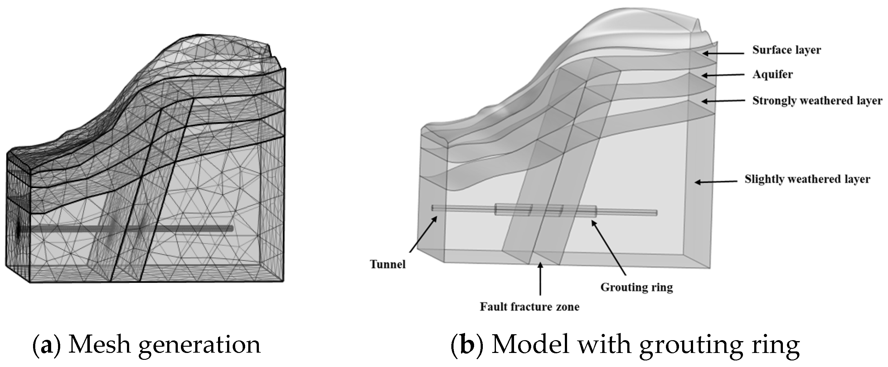
The generated seepage simulation model is shown in Figure 1. The numerical model was discretized using physics-controlled meshing in COMSOL Multiphysics 6.4. Local mesh refinement was applied around the tunnel and the fault fracture zone to improve the accuracy of seepage simulation in critical regions. The final mesh consisted of 10,448 domain elements, 3093 boundary elements, and 408 edge elements, including 10,448 tetrahedral elements and 3093 triangular elements.

The steady-state seepage equations were solved using the stationary solver in COMSOL Multiphysics. A fully coupled solution scheme was adopted, and the relative tolerance was set to 0.0001.

The linear system was solved using the default direct solver. The solution was considered converged when the residuals of the governing equations satisfied the prescribed tolerance and no further noticeable change in the calculated tunnel inflow was observed.

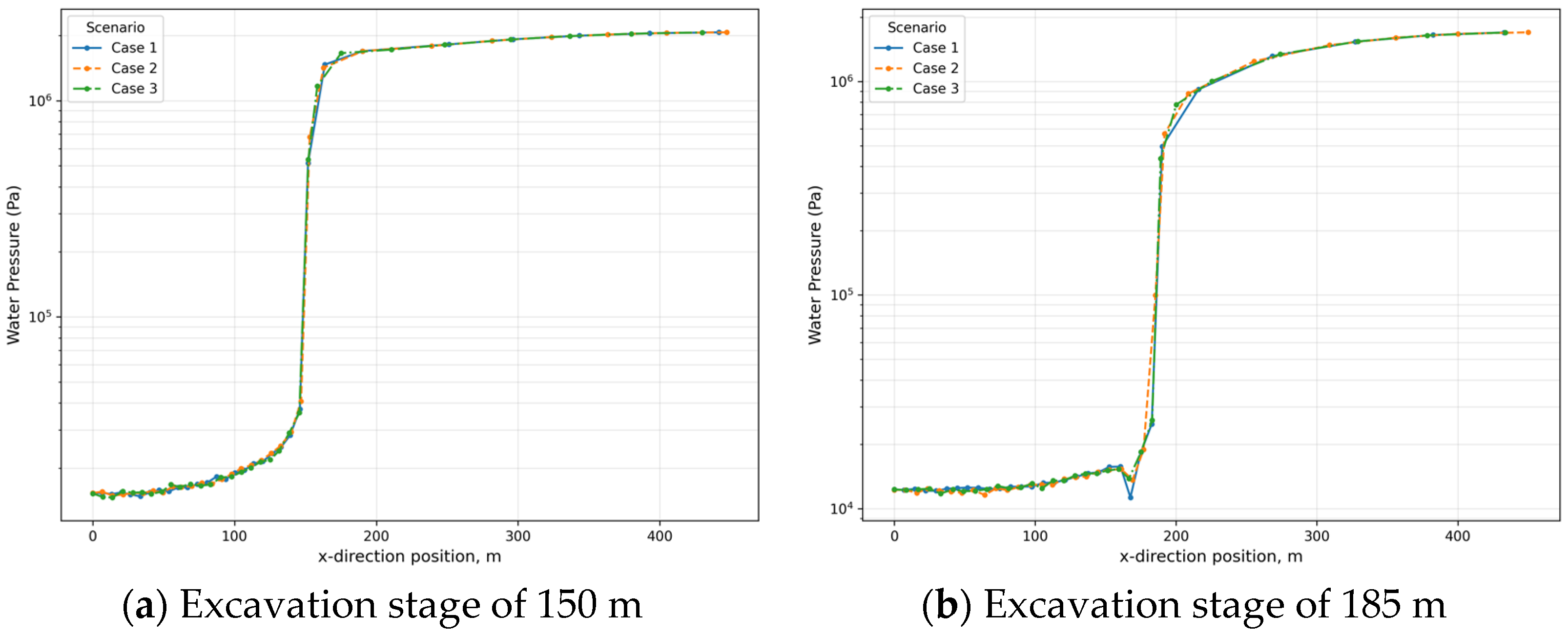
A mesh-independence check was further conducted using the non-grouted numerical model. Three mesh densities were considered, namely Case 1, Case 2, and Case 3, with the mesh density gradually decreasing from Case 1 to Case 3. Case 3 was adopted for the subsequent simulations considering both computational accuracy and efficiency. The water-pressure distributions along the x direction at monitoring points located 0.2 m above the tunnel crown were compared at two representative excavation stages, namely 150 m and 185 m, as shown in Figure 2.

The results show that the pressure-distribution curves obtained under the three mesh densities are highly consistent, including the low-pressure region, the rapid pressure-increase zone, and the high-pressure plateau. This indicates that the calculated hydraulic response is insensitive to further mesh refinement, and that the adopted mesh provides sufficient numerical accuracy for the subsequent parametric simulations.

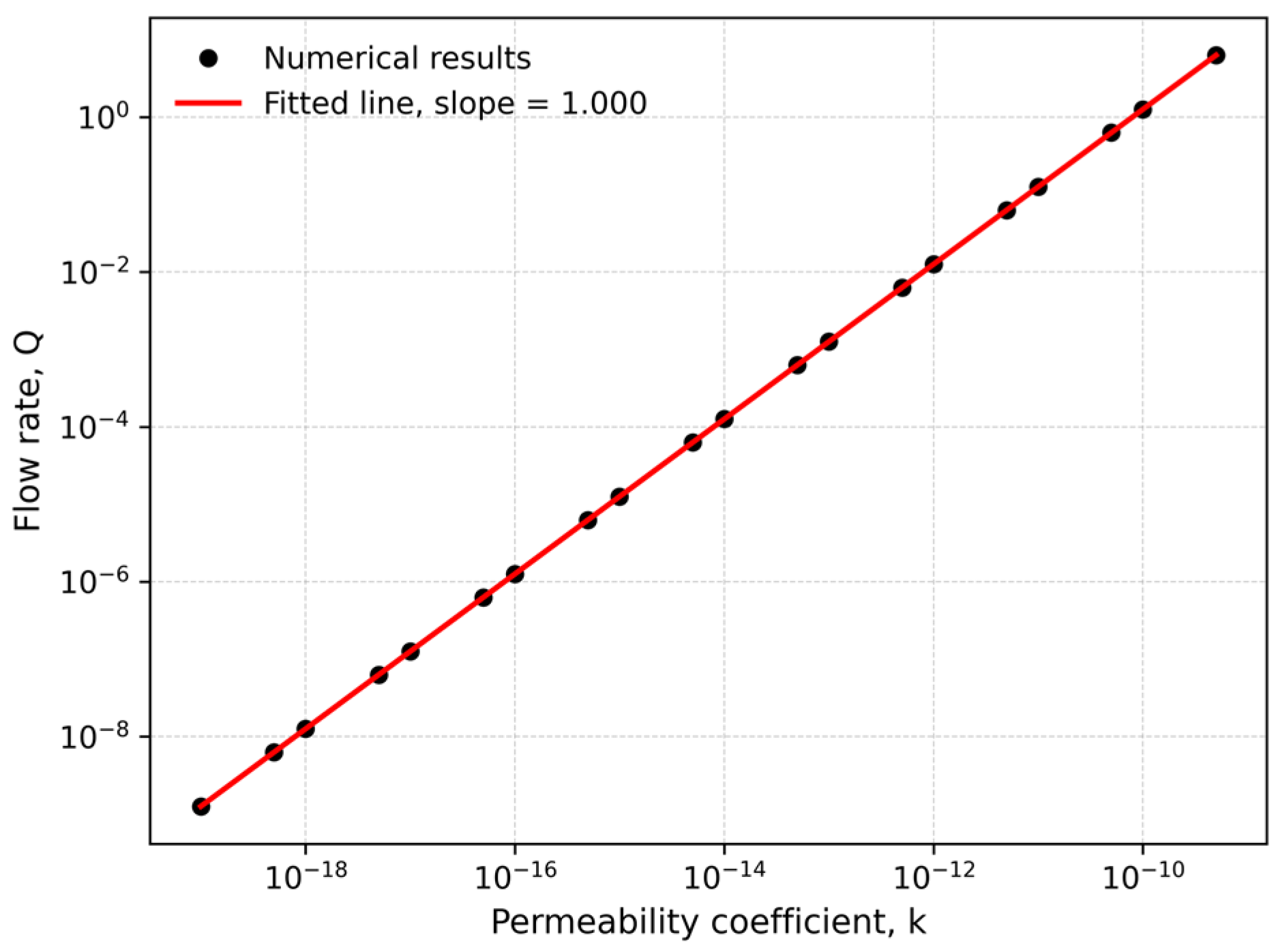
A cylindrical seepage model with a radius of 0.1 m and a height of 0.5 m was established to verify the relationship between permeability coefficient and flow rate. The lateral boundary of the cylinder was set as impermeable, while a water pressure of 1 MPa was applied at the top surface and the bottom surface was assigned a pressure of 0 MPa. The computed flow rates under different permeability coefficients are shown in Figure 3.

The results show that the flow rate increases linearly with the permeability coefficient under the same hydraulic boundary conditions. Specifically, when the permeability coefficient increases by one order of magnitude, the corresponding flow rate also increases by one order of magnitude. This indicates that the numerical results are consistent with Darcy’s law, confirming the reliability of the seepage simulation setup.

2.2. Grouting Ring Design and Orthogonal Experimental Scheme

Based on the three-dimensional geological seepage model containing the fault fracture zone, a cylindrical grouting ring was arranged around the tunnel to investigate the influence of grouting reinforcement on the seepage field and tunnel water inflow. The grouting ring was used to represent the water-blocking reinforcement zone formed by advance grouting during tunnel construction. By varying the geometric and hydraulic parameters of the grouting ring, the water-control effects of different grouting schemes were quantitatively evaluated.

Orthogonal experimental design is a multifactor and multilevel experimental design method based on mathematical statistics and the principle of balanced dispersion. By using a limited number of representative test cases instead of exhaustive full-factorial combinations, this method can substantially reduce the computational burden while preserving balanced coverage of the selected factor levels. It also helps overcome the limitation of conventional single-factor analysis, which cannot effectively reflect the coupled effects among multiple parameters.

Compared with random sampling, orthogonal experimental design provides more balanced coverage of factor levels under a limited number of simulations. Compared with Latin hypercube sampling, an orthogonal array is easier to implement for discrete engineering parameter levels and facilitates subsequent range analysis and correlation analysis. However, orthogonal experimental design may not fully cover continuous parameter spaces, which represents a limitation of the current database.

In this study, the water inflow per unit tunnel length was selected as the target indicator. Based on previous parameter sensitivity analysis and the seepage-control mechanism of grouted fault tunnels, four parameters that exert primary control on tunnel water inflow were selected as orthogonal experimental factors: grouting ring permeability coefficient, grouting ring thickness, surrounding rock permeability coefficient, and advance grouting length from the fault. These factors respectively represent the hydraulic resistance of the grouting reinforcement zone, the radial water-blocking thickness around the tunnel, the permeability condition of the surrounding rock, and the longitudinal grouting range before the tunnel reaches the fault zone.

Each factor was assigned five levels. The parameter ranges were determined according to the Code for Design of Railway Tunnels, the Code for Design of Highway Tunnels, the geological investigation report of the Yinggeling Tunnel, and commonly used parameter intervals in engineering practice. This setting improves the engineering relevance of the numerical simulations while keeping the number of numerical cases computationally manageable. A five-level orthogonal array with 25 representative parameter combinations was adopted for the experimental design. Four columns of the orthogonal array were assigned to the selected hydraulic and grouting factors, yielding a total of 25 numerical simulation cases. The detailed factor levels are presented in

Table 2. Factors and levels used in the orthogonal experimental design.

Factor Symbol	Influencing Factor	Level 1	Level 2	Level 3	Level 4	Level 5
A	Grouting ring thickness (m)	3	4	5	6	7
B	Grouting ring permeability coefficient (cm/s)	1 × 10−6	2 × 10−6	5 × 10−6	10 × 10−6	50 × 10−6
C	Advance grouting length from fault (m)	30	40	50	60	70
D	Surrounding rock permeability coefficient (cm/s)	1 × 10−5	2.5 × 10−5	5 × 10−5	10 × 10−5	20 × 10−5

.

It should be noted that the orthogonal experimental scheme was used only to define the four basic hydraulic and grouting parameters of each numerical simulation case. In the subsequent database construction, additional excavation-position variables were introduced when extracting water inflow records at different excavation positions along the tunnel axis. These excavation-position variables were not independent orthogonal design factors, but derived descriptors used to characterize the spatial relationship between the excavation face, the grouting zone, and the fault fracture zone. Their definitions are provided in Section 2.3.

2.3. Sample Database Construction and Input Variable Definition

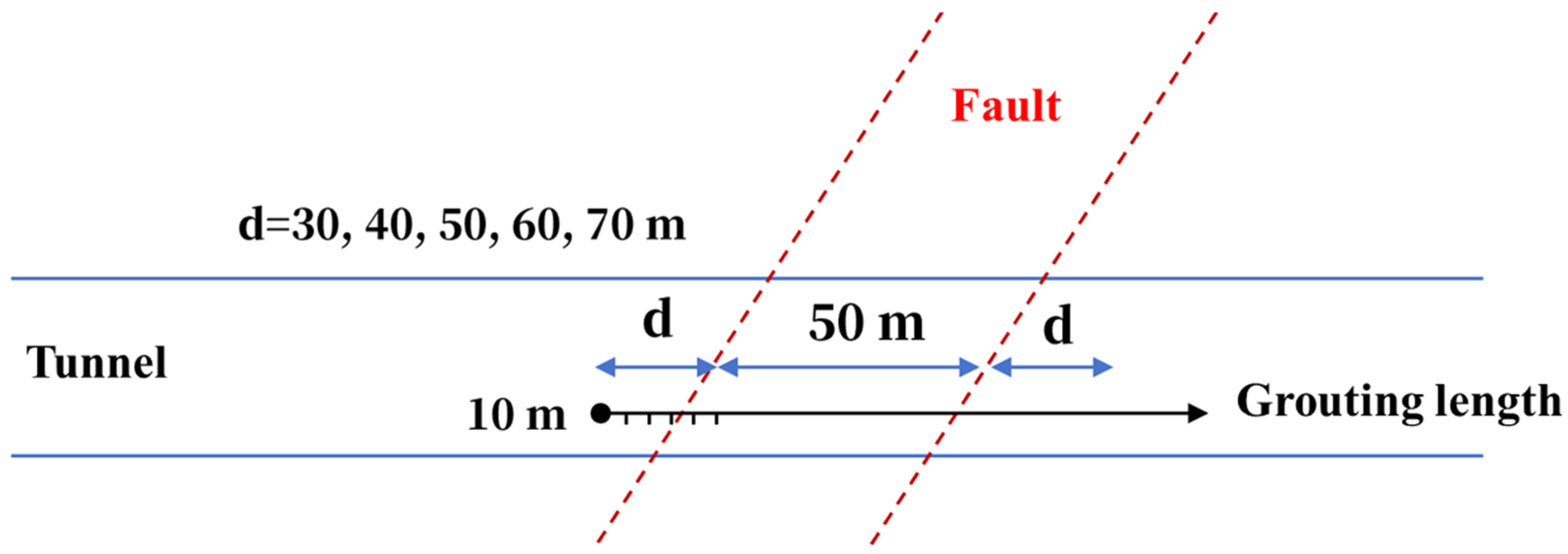
For all simulation cases, the geometric dimensions, boundary conditions, seepage assumptions, and material constitutive relationships of the numerical model were kept identical. A parametric sweep was adopted to simulate tunnel water inflow under different grouting and hydraulic conditions. The four parameters varied among the orthogonal simulation cases were the grouting ring permeability coefficient, grouting ring thickness, surrounding rock permeability coefficient, and advance grouting length from the fault. Because the relative distance between the excavation face and the fault fracture zone directly affects water inflow during tunnel excavation, the water inflow at different excavation positions was calculated stepwise at 10 m intervals along the tunnel axis for each orthogonal case. The corresponding water inflow per unit tunnel length was then extracted. The distribution of the calculation positions of water inflow per linear meter is shown in Figure 4.

Specifically, cases with an advance grouting length of 30 m from the fault generated 13 valid water inflow records at different excavation positions, whereas cases with advance grouting lengths of 40 m, 50 m, 60 m, and 70 m generated 15, 17, 19, and 21 valid records, respectively. Since each advance grouting length level appeared in five orthogonal simulation cases, the 25 orthogonal simulation cases produced 425 valid data records in total, as summarized in

Table 3. Number of valid samples generated under different advance grouting lengths.

Advance Grouting Length from Fault	Valid Records per Simulation Case	Number of Simulation Cases	Total Samples
30 m	13	5	65
40 m	15	5	75
50 m	17	5	85
60 m	19	5	95
70 m	21	5	105
Total	—	25	425

.

In addition to the four orthogonal design parameters, two excavation-position variables were introduced to describe the spatial relationship between the excavation face, the grouting zone, and the fault fracture zone. The first variable was the excavation-position distance from the grouting starting position, which was recorded at 10 m intervals. This variable reflects the relative advancement of the excavation face within the grouted and fault-influenced region. The second variable was the excavation-position category. According to the spatial relationship between the excavation face and the fault fracture zone, this category was coded as 1, 2, and 3, representing before the fault zone, within the fault zone, and behind the fault zone, respectively.

Therefore, the final machine learning dataset contained six input variables and one output variable. The six input variables included the grouting ring permeability coefficient, grouting ring thickness, surrounding rock permeability coefficient, advance grouting length from the fault, excavation-position distance from the grouting starting position, and excavation-position category. The output variable was the water inflow per unit tunnel length, expressed in m³/(m·d). The definitions, units, and physical meanings of these variables are summarized in

Table 4. Influencing factors and output variable used in the machine learning dataset.

Category	Variable	Symbol	Unit	Type	Description
Grouting parameter	Grouting ring permeability coefficient	kg	cm/s	Continuous	Hydraulic conductivity of the grouting ring
Grouting parameter	Grouting ring thickness	tg	m	Continuous	Thickness of the grouting reinforcement ring
Geological parameter	Surrounding rock permeability coefficient	kr	cm/s	Continuous	Hydraulic conductivity of the surrounding rock mass
Grouting design parameter	Advance grouting length from the fault	Lg	m	Continuous	Length of the advance grouting section before the fault zone
Excavation-related parameter	Excavation-position distance from the grouting starting position	De	m	Continuous	Distance from the grouting starting position to the current excavation position
Excavation-related parameter	Excavation-position category	Ce	—	Categorical	Excavation zone relative to the fault
Output	Water inflow per unit tunnel length	q	m3/(m·d)	Continuous	Simulated water inflow normalized by tunnel length

.

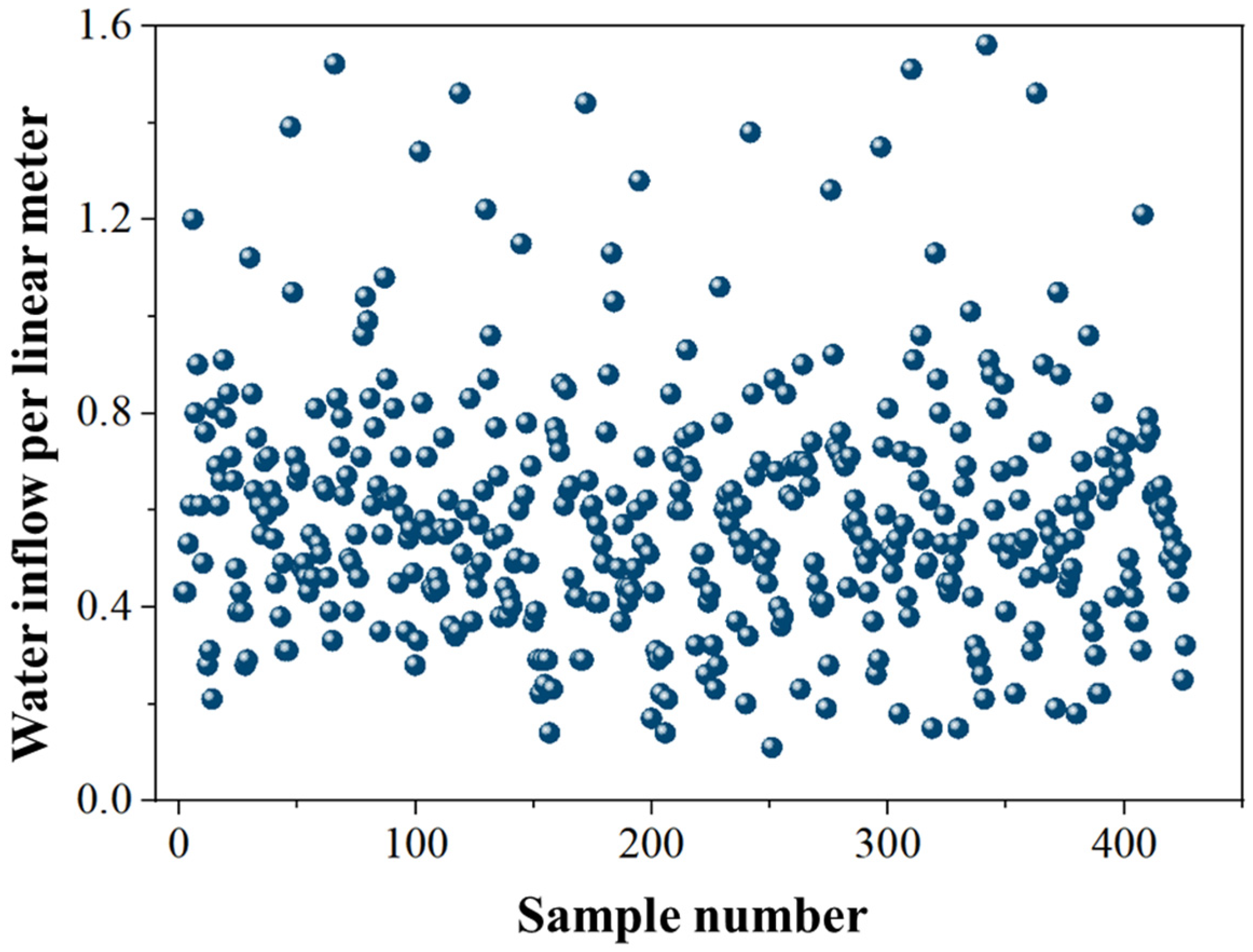
The distribution of the simulated water inflow per unit tunnel length for all samples is shown in Figure 5.

It should be emphasized that the 425 samples were generated from 25 orthogonal numerical simulation cases at different excavation positions. Therefore, the samples have physical consistency and can reflect the spatial variation in water inflow as the excavation face approaches, passes through, and moves away from the fault fracture zone. However, they should not be regarded as 425 completely independent field cases. Samples belonging to the same orthogonal simulation case share the same basic hydraulic and grouting parameter combination and may therefore be correlated. To reduce information leakage in subsequent machine learning modeling, the orthogonal simulation case ID was used as the grouping variable. During grouped validation, samples from the same simulation case were assigned exclusively to either the training set or the test set.

2.4. Data Characteristic Analysis

Before machine learning modeling, data characteristic analysis was conducted to clarify the relationships between the input variables and the target variable and to provide an interpretive basis for subsequent model construction and result discussion. In this section, exploratory analysis of the 425 samples was conducted from two perspectives: parameter correlation and variable clustering. Pearson correlation analysis [27] was used to quantify the direction and strength of the linear relationships among variables. Hierarchical clustering [28] was further used to identify similarity patterns among hydraulic parameters and engineering control parameters. By combining these two methods, the dominant factors influencing tunnel water inflow and the grouping characteristics of different variables were preliminarily identified.

The analyzed variables included six input variables and one output variable. The input variables were the grouting ring permeability coefficient, grouting ring thickness, surrounding rock permeability coefficient, advance grouting length from the fault, excavation-position distance from the grouting starting position, and excavation-position category. The output variable was the water inflow per unit tunnel length. The excavation-position category was coded as 1, 2, and 3, representing before the fault zone, within the fault zone, and behind the fault zone, respectively. Therefore, the correlation result for this variable should be interpreted as an ordinal trend rather than a strict continuous linear relationship.

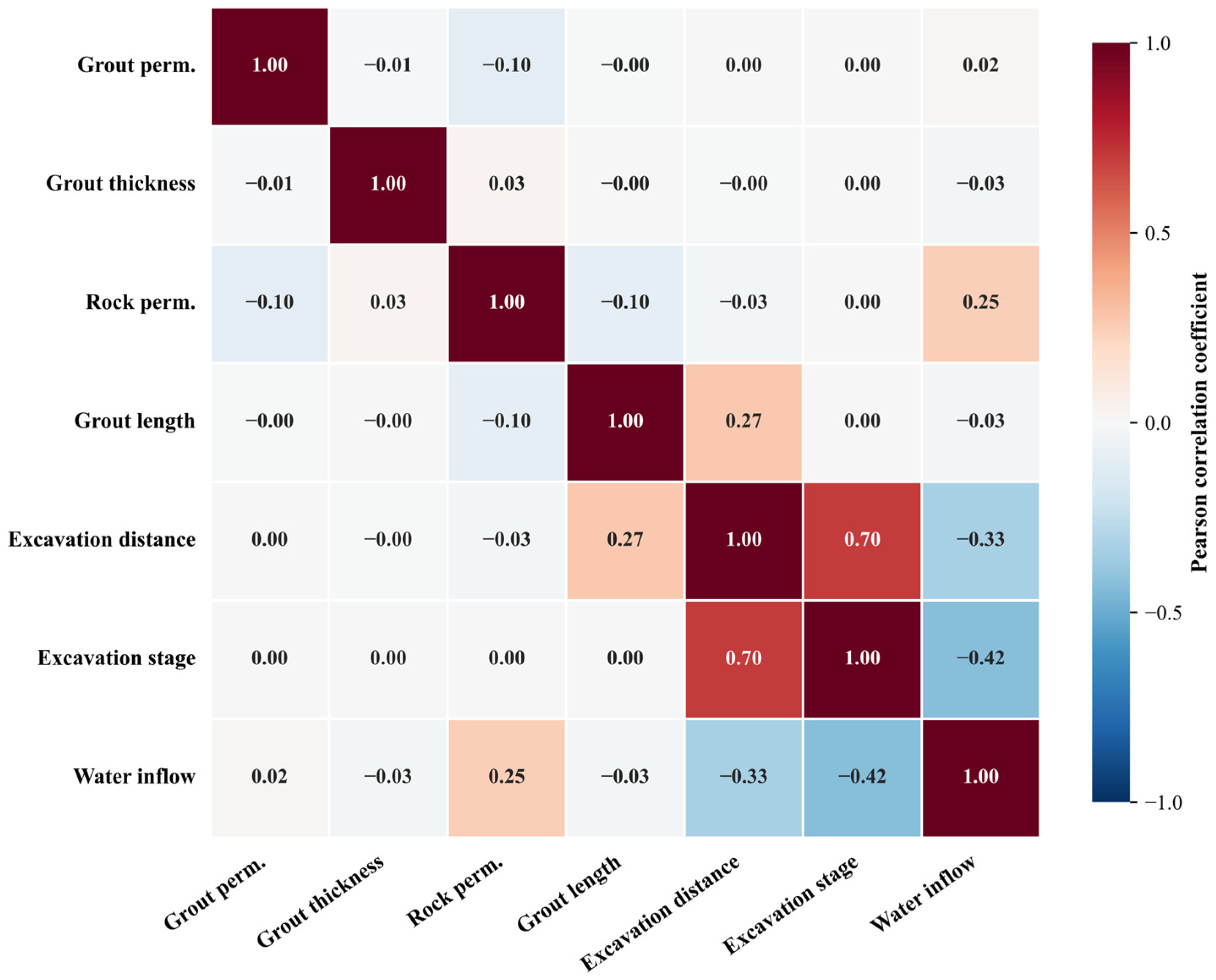
As shown in Figure 6, most individual input variables exhibited weak to moderate linear correlations with water inflow per unit tunnel length. Among the grouting-related variables, the grouting ring permeability coefficient, grouting ring thickness, and advance grouting length showed very weak correlations with water inflow, with coefficients of approximately 0.02, −0.03, and −0.03, respectively. This indicates that the direct linear effects of individual grouting parameters were not obvious within the present orthogonal simulation dataset.

The surrounding rock permeability coefficient showed a weak positive correlation with water inflow, with a coefficient of approximately 0.25, suggesting that higher surrounding rock permeability tended to promote tunnel water inflow. Compared with the grouting-related variables, the excavation-related variables showed more noticeable correlations. Excavation distance and excavation stage were negatively correlated with water inflow, with coefficients of approximately −0.33 and −0.42, respectively. In addition, excavation distance was strongly positively correlated with excavation stage, with a coefficient of approximately 0.70. Since excavation stage was encoded as a categorical variable, this correlation should be interpreted as an ordinal trend rather than a strict continuous linear relationship.

Overall, the correlation analysis indicates that water inflow could not be explained by any single linear factor. Instead, it was likely governed by coupled and nonlinear interactions among geological conditions, grouting parameters, and excavation-position descriptors. Therefore, nonlinear machine learning models were needed to capture the complex relationship between the selected input variables and water inflow.

2.5. Computational Environment and Implementation

As summarized in

Table 5. Technological stack used in this study.

Component	Software/ Library	Version	Purpose in This Study
Programming language	Python	3.12.10	Implementation of data processing, machine-learning modeling, hyperparameter optimization, and visualization
Numerical computation	NumPy	2.4.2	Numerical array operations and mathematical calculations
Data processing	Pandas	3.0.1	Data loading, preprocessing, cleaning, and result organization
Machine-learning framework	scikit-learn	1.9.0	Implementation of SVM, Random Forest, grouped data splitting, preprocessing pipelines, and evaluation metrics
Gradient boosting model	XGBoost	3.2.0	Implementation of the XGBoost regression model
Gradient boosting model	CatBoost	1.2.10	Implementation of the CatBoost regression model and optimized CatBoost models
Bayesian optimization	Optuna	4.8.0	Bayesian hyperparameter optimization based on the TPE sampler
Statistical analysis	SciPy	1.17.1	Statistical tests, including paired comparison analysis
Visualization	Matplotlib	3.10.8	Generation of prediction plots, residual plots, and performance figures
Visualization	Seaborn	0.13.2	Generation of correlation heatmaps and metric heatmaps

, all numerical analyses and machine-learning experiments were implemented in Python 3.12.10. NumPy and Pandas were used for numerical computation and data preprocessing. The SVM and Random Forest models, grouped data splitting, preprocessing pipelines, and evaluation metrics were implemented using scikit-learn. XGBoost and CatBoost were used to construct the corresponding gradient boosting regression models. Bayesian optimization was performed using Optuna, while random search, the Osprey Optimization Algorithm, and the Grey Wolf Optimizer were implemented in Python under the same evaluation budget. Matplotlib 3.10.8 and Seaborn 0.13.2 were used for generating the figures and heatmaps. Fixed random seeds were used in the grouped validation and model training procedures to improve reproducibility.

3. Prediction Model Construction and Optimization

3.1. Dataset Division, Preprocessing, and Validation Framework

The dataset division, preprocessing, and validation framework were designed as follows.

• Input and output variables
  The six input variables and one output variable defined in Section 2.3 were used for machine learning modeling. The input variables included four hydraulic and grouting parameters and two excavation-position descriptors. The excavation-position category was transformed using one-hot encoding before model training to avoid imposing an artificial ordinal relationship among the three excavation zones.
• Repeated grouped hold-out validation
  To reduce the uncertainty associated with a single train–test split, ten repeated grouped hold-out validations were conducted using random seeds from 1 to 10. In each repetition, the dataset was divided into a training set and an independent test set at the simulation-case level rather than at the individual-sample level. The orthogonal simulation case ID was used as the grouping variable, and all samples belonging to the same simulation case were assigned exclusively to either the training set or the test set.
  In each grouped split, 18 simulation cases were used for training, and the remaining 7 simulation cases were used for independent testing. Because the number of samples extracted from each simulation case varied with the advance grouting length, the exact numbers of training and test samples varied slightly among different repeated splits. This grouped splitting strategy ensured that the test set contained unseen hydraulic and grouting parameter combinations at the simulation-case level, thereby reducing information leakage and providing a stricter evaluation of model generalization ability.
• Model training and hyperparameter optimization
  For the baseline models, each model was trained on the grouped training set and evaluated on the corresponding independent grouped test set. For the optimized CatBoost models, hyperparameter optimization was performed only within the grouped training set. Specifically, five-fold grouped cross-validation was conducted on the training cases for each candidate hyperparameter combination, and the mean validation R² was used as the fitness value.
  After the optimal hyperparameter combination was determined for each optimization algorithm, the final CatBoost model was retrained using the entire grouped training set and then evaluated once on the independent grouped test set. The final performance was reported as the mean ± standard deviation of the evaluation metrics over the ten repeated grouped train–test splits.
• Data preprocessing
  Differentiated preprocessing strategies were adopted according to the characteristics of different algorithms [29]. The SVM model is sensitive to feature scales; therefore, Z-score standardization was applied to the input features when training SVM. To avoid information leakage, the mean and standard deviation used for standardization were calculated only from the training set and then applied to the corresponding test set. Random Forest, XGBoost, and CatBoost are tree-based ensemble learning models and are generally insensitive to feature scaling. Therefore, no standardization was applied to these models so that the original physical meanings of the input variables could be preserved.

3.2. Model Evaluation Metrics

To comprehensively evaluate the prediction performance of the models, five evaluation metrics commonly used for regression tasks were selected [30]: Mean Absolute Error (MAE), Mean Square Error (MSE), Root Mean Square Error (RMSE), Mean Absolute Percentage Error (MAPE), and the coefficient of determination (R²). The formulas for these metrics are expressed as follows:

$$MAE={\displaystyle \frac{1}{m}}{\displaystyle \sum _{i=1}^m}\left(\left|y_i-f\left(x_i\right)\right|\right)$$

(3)

$$MSE={\displaystyle \frac{1}{m}}{\displaystyle \sum _{i=1}^m}{\left(y_i-f\left(x_i\right)\right)}^2$$

(4)

$$RMSE=\sqrt{{\displaystyle \frac{1}{m}}{\displaystyle \sum _{i=1}^m}{\left(y_i-f\left(x_i\right)\right)}^2}$$

(5)

$$MAPE={\displaystyle \frac{1}{m}}{\displaystyle \sum _{i=1}^m}\left(\left|{\displaystyle \frac{y_i-f\left(x_i\right)}{y_i}}\right|\right)\times 100\%$$

(6)

$$R^2=1-{\displaystyle \frac{MSE\left(y_i,f\left(x_i\right)\right)}{\frac{1}{m}{{\displaystyle {\sum }_{i=1}^m}\left(y_i-\overline{y}\right)}^2}}$$

(7)

where $y_i$ is the true value of water inflow per linear meter, $f\left(x_i\right)$ is the predicted value of water inflow per linear meter, $\overline{y}$ denotes the mean of the true values of water inflow per linear meter, and m is the number of samples. $MAE$ is used to evaluate the closeness between the predicted results and the true dataset; the smaller its value, the better the fitting effect. $MSE$ calculates the mean of the squared errors between the fitted data and the original data at corresponding sample points; the smaller its value, the better the fitting effect, and $RMSE$ is the square root of $MSE$. MAPE reflects the relative prediction error in percentage form. The coefficient of determination (R²) measures the proportion of variance in the true values that can be explained by the model. A higher coefficient of determination indicates better explanatory and predictive performance.

3.3. Baseline Machine Learning Models

In this study, four classical machine learning algorithms were selected to construct tunnel water inflow prediction models, covering three mainstream algorithm categories: kernel-based methods, bagging ensemble learning, and gradient boosting decision trees. Through repeated validation, the model with the best overall generalization performance was selected as the base model for subsequent hyperparameter optimization. The core principles of each algorithm are described as follows.

• Support Vector Machine Regression (SVM):
  SVM is a machine learning algorithm grounded in the principle of structural risk minimization. Its core idea is to map samples that are linearly inseparable in a low-dimensional space into a high-dimensional feature space through a kernel function and construct an optimal regression hyperplane in this high-dimensional space. In this way, the deviations of the samples from the hyperplane are minimized. SVM performs well in nonlinear fitting problems with small samples and high-dimensional data and possesses a certain degree of noise immunity. However, its computational complexity increases substantially with the number of samples, and its fitting capability for large-sample datasets may be weaker than that of ensemble learning models.
• Random Forest (RF):
  RF is an ensemble learning algorithm based on the Bagging framework. Its core principle is to draw multiple subsets from the original training set through bootstrap sampling, independently train a decision tree for each subset, and obtain the final output by averaging the prediction results of all decision trees. Through the ensemble effect of multiple trees, Random Forest can reduce the overfitting risk of individual decision trees. It is robust to data noise and outliers, has relatively high training efficiency, and can provide feature importance rankings, making it suitable for nonlinear tabular data commonly encountered in geotechnical engineering.
• eXtreme Gradient Boosting (XGBoost):
  XGBoost is an ensemble learning algorithm based on the gradient boosting framework. It optimizes the loss function using second-order Taylor expansion and introduces a regularization term to control model complexity, thereby improving fitting accuracy and overfitting resistance. XGBoost has strong fitting ability for nonlinear relationships; however, it is highly sensitive to hyperparameter settings. When the hyperparameters are improperly configured, overfitting may occur, with good fitting performance on the training set but limited generalization ability on the test set.
• Categorical Boosting (CatBoost):
  CatBoost is a gradient boosting decision tree algorithm designed to improve the handling of categorical features and reduce prediction bias. It alleviates gradient bias and prediction shift in traditional gradient boosting decision trees by adopting an ordered boosting mechanism and an automatic categorical feature encoding strategy. CatBoost usually shows stable performance on tabular data, although its generalization ability still depends on dataset size and hyperparameter settings.

3.4. CatBoost Hyperparameter Optimization Strategies and Implementation Details

Based on the repeated grouped validation results of the baseline models, CatBoost was selected as the base model for further hyperparameter optimization. CatBoost is a gradient boosting decision tree algorithm that has strong nonlinear fitting capability and can effectively capture complex interactions among hydraulic parameters, grouting design variables, and excavation-position information. Its prediction performance is influenced by several key hyperparameters, including the number of boosting iterations, tree depth, learning rate, L2 regularization coefficient, and bagging temperature. Therefore, appropriate hyperparameter optimization is necessary to improve the balance between fitting capability and generalization performance. The search space used for all optimization methods is shown in

Table 6. CatBoost hyperparameter search space used for all optimization methods.

Hyperparameter	Type	Search Space	Description
iterations	Integer	100–800	Number of boosting iterations
depth	Integer	2–10	Depth of each regression tree
learning_rate	Continuous	0.01–0.30	Step size shrinkage used in boosting
l2_leaf_reg	Continuous	1.0–20.0	L2 regularization coefficient of leaf values
bagging_temperature	Continuous	0.0–1.0	Parameter controlling the intensity of Bayesian bootstrap sampling

.

In this study, four hyperparameter optimization strategies were compared for CatBoost: Random Search (RS), Bayesian Optimization (BO), Osprey Optimization Algorithm (OOA) [31], and Grey Wolf Optimizer (GWO). RS randomly samples candidate hyperparameter combinations from a predefined search space and is commonly used as a simple but effective baseline optimization method. BO was implemented using Optuna with the Tree-structured Parzen Estimator (TPE) sampler, which sequentially models promising and non-promising regions of the hyperparameter space and samples new candidates accordingly. OOA is a bio-inspired swarm intelligence algorithm that simulates the predation behavior of ospreys and attempts to balance global exploration and local exploitation. GWO is another swarm intelligence algorithm inspired by the social hierarchy and hunting behavior of grey wolves and has been widely applied in engineering optimization problems.

The implementation settings of the four optimization methods are summarized in

Table 7. Implementation settings of the four CatBoost hyperparameter optimization methods.

Method	Implementation	Main Settings	Evaluation Budget	Stopping Criterion
RS	ParameterSampler	Random sampling from the predefined search space	200	200 evaluations
BO	Optuna TPE sampler	200 sequential trials	200	200 trials
OOA	Population-based OOA	Population size = 20; two update phases; evaluation-budget control	200	200 evaluations
GWO	Grey Wolf Optimizer	Population size = 20; maximum iterations = 10	200	200 evaluations

. To ensure a fair comparison, all methods were constrained to the same evaluation budget of 200 candidate hyperparameter configurations for each grouped train–test split.

For OOA and GWO, each candidate solution was represented as a five-dimensional vector corresponding to the five CatBoost hyperparameters. During the search process, candidate positions were updated in a continuous search space. Before CatBoost training, integer hyperparameters, including iterations and depth, were rounded to the nearest integer. Continuous hyperparameters, including learning_rate, l2_leaf_reg, and bagging_temperature, were directly used after boundary correction. All hyperparameter values were clipped to the predefined lower and upper bounds. If a candidate solution exceeded the feasible search range, it was projected back to the boundary of the search space.

To ensure reproducibility, the outer grouped train–test split seeds were set from 1 to 10. The random state of the CatBoost model was fixed at 42 in all experiments. The stopping criterion for all optimization methods was reaching the predefined budget of 200 candidate evaluations. No early stopping or parameter selection based on the independent test set was used.

The computational cost was recorded as the elapsed time required for hyperparameter optimization and final model evaluation in each repeated split. In addition, the convergence history of each optimization run was recorded by storing the grouped cross-validation R² value of each evaluated candidate solution. The best cross-validation R² achieved up to each candidate evaluation was used to characterize the convergence behavior of different optimization methods.

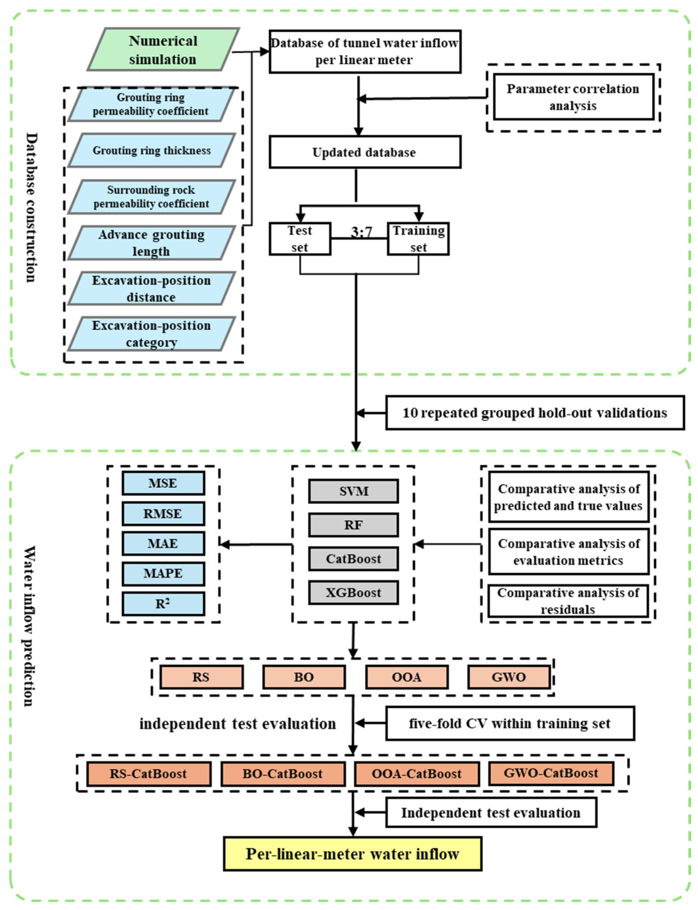
The technical roadmap of the model construction and CatBoost hyperparameter optimization framework is shown in Figure 7.

3.5. Statistical Analysis

To further examine whether the differences among the CatBoost optimization methods were statistically significant, paired t-tests were conducted based on the test metrics obtained from the ten repeated grouped train–test splits. Paired t-tests were conducted to compare OOA-CatBoost with the unoptimized CatBoost model and the other optimized CatBoost models. A significance level of 0.05 was adopted. When p < 0.05, the performance difference was considered statistically significant; otherwise, there was insufficient evidence to conclude a statistically significant difference.

4. Model Prediction Results and Performance Analysis

4.1. Repeated Validation and Performance Comparison of Baseline Models

To evaluate the prediction performance and generalization ability of different machine learning models, four baseline models, namely SVM, RF, XGBoost, and CatBoost, were established for tunnel water inflow prediction. The six input variables defined in Section 2.3 were used as model inputs, and the water inflow per unit tunnel length was used as the target output variable.

As described in Section 3.1, the baseline models were evaluated using ten repeated grouped hold-out validations with the orthogonal simulation case ID as the grouping variable. This strategy ensured that samples from the same simulation case were not simultaneously included in the training and test sets.

The mean and standard deviation of five evaluation metrics, including R², MAE, MSE, RMSE, and MAPE, were calculated for both the training and test sets over the 10 repeated grouped splits. The results are listed in

Table 8. Training and test performance of baseline models under 10 repeated grouped hold-out validations.

Model	Dataset	R2	MAE	MSE	RMSE	MAPE
CatBoost	Training set	0.9661 ± 0.0036	0.0341 ± 0.0014	0.0020 ± 0.0002	0.0451 ± 0.0020	6.9247 ± 0.3180
	Test set	0.6209 ± 0.0405	0.1084 ± 0.0079	0.0243 ± 0.0027	0.1555 ± 0.0085	22.9606 ± 3.3508
Random Forest	Training set	0.9501 ± 0.0032	0.0388 ± 0.0006	0.0030 ± 0.0001	0.0548 ± 0.0013	8.3865 ± 0.2660
	Test set	0.6055 ± 0.0349	0.1095 ± 0.0055	0.0252 ± 0.0022	0.1587 ± 0.0069	23.6706 ± 3.1706
SVM	Training set	0.6031 ± 0.0150	0.1065 ± 0.0022	0.0239 ± 0.0010	0.1545 ± 0.0031	20.3155 ± 0.6381
	Test set	0.3639 ± 0.0639	0.1442 ± 0.0087	0.0408 ± 0.0049	0.2016 ± 0.0120	28.8764 ± 2.9499
XGBoost	Training set	0.9993 ± 0.0002	0.0046 ± 0.0006	0.0000 ± 0.0000	0.0063 ± 0.0007	0.8932 ± 0.1231
	Test set	0.5462 ± 0.0661	0.1169 ± 0.0098	0.0291 ± 0.0045	0.1700 ± 0.0129	24.4712 ± 3.5478

.

The results show that the CatBoost model achieved the best overall performance on the test set among the four baseline models. Specifically, CatBoost obtained the highest average test R² of 0.6209 ± 0.0405, while its MAE, MSE, RMSE, and MAPE were 0.1084 ± 0.0079, 0.0243 ± 0.0027, 0.1555 ± 0.0085, and 22.9606 ± 3.3508, respectively. These error metric values were lower than those of the other three models, indicating that CatBoost had a relatively better ability to capture the nonlinear relationship between tunnel water inflow and multiple coupled influencing factors in the present dataset.

Random Forest showed the second-best test performance, with a test R² of 0.6055 ± 0.0349, while its MAE, MSE, RMSE, and MAPE were 0.1095 ± 0.0055, 0.0252 ± 0.0022, 0.1587 ± 0.0069, and 23.6706 ± 3.1706, respectively.

XGBoost exhibited the strongest fitting ability on the training set. Its training R² reached 0.9993 ± 0.0002, and the training errors were nearly zero. However, its test R² decreases significantly to 0.5462 ± 0.0661, while the test MAE and RMSE increase to 0.1169 ± 0.0098 and 0.1700 ± 0.0129, respectively. This indicates that extreme gradient boosting tended to overfit the training samples and showed limited generalization ability for unseen samples. The relatively large standard deviation of the test R² also suggests that XGBoost was more sensitive to different data partitions.

In contrast, SVM exhibited the weakest predictive performance among the four baseline models. Its test R² was only 0.3639 ± 0.0639, and its MAE, MSE, RMSE, and MAPE were all higher than those of the other models. The relatively low R² values on both the training and test sets indicate that SVM had limited ability to describe the complex nonlinear mapping relationship between water inflow and the input variables. Therefore, SVM was more likely to suffer from underfitting rather than overfitting in this prediction task.

Since several samples in the dataset had relatively small water inflow values, MAPE was more sensitive to local prediction deviations. Therefore, R², MAE, and RMSE were regarded as the primary evaluation metrics in this study, while MAPE was used as an auxiliary indicator. Based on the comprehensive comparison of the repeated validation results, the overall prediction performance of the four baseline models on the test set can be ranked as follows:

$$\mathrm{C}\mathrm{a}\mathrm{t}\mathrm{B}\mathrm{o}\mathrm{o}\mathrm{s}\mathrm{t}>\mathrm{R}\mathrm{F}>\mathrm{X}\mathrm{G}\mathrm{B}\mathrm{o}\mathrm{o}\mathrm{s}\mathrm{t}>\mathrm{S}\mathrm{V}\mathrm{M}$$

Therefore, CatBoost was selected as the base model for subsequent hyperparameter optimization.

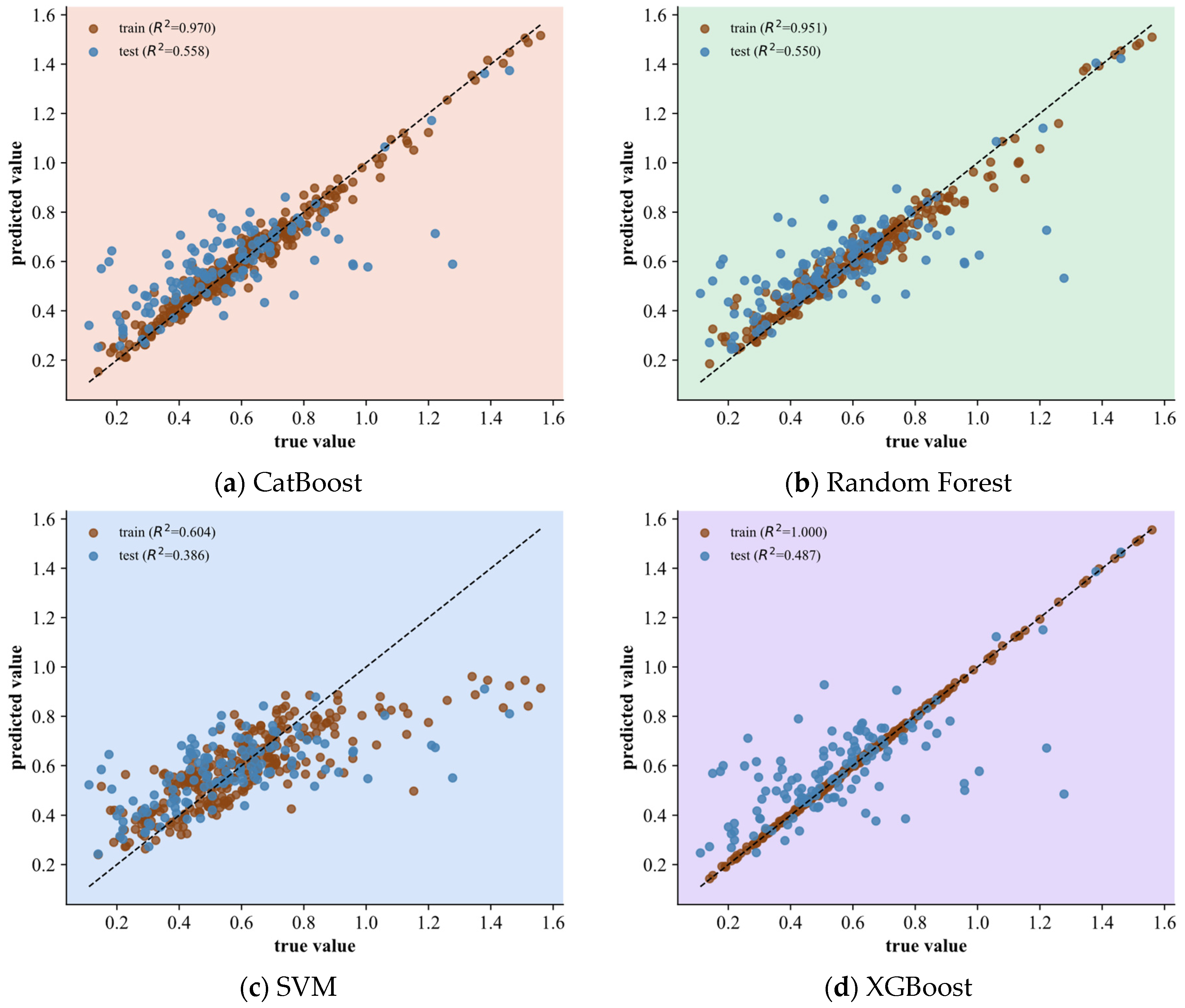
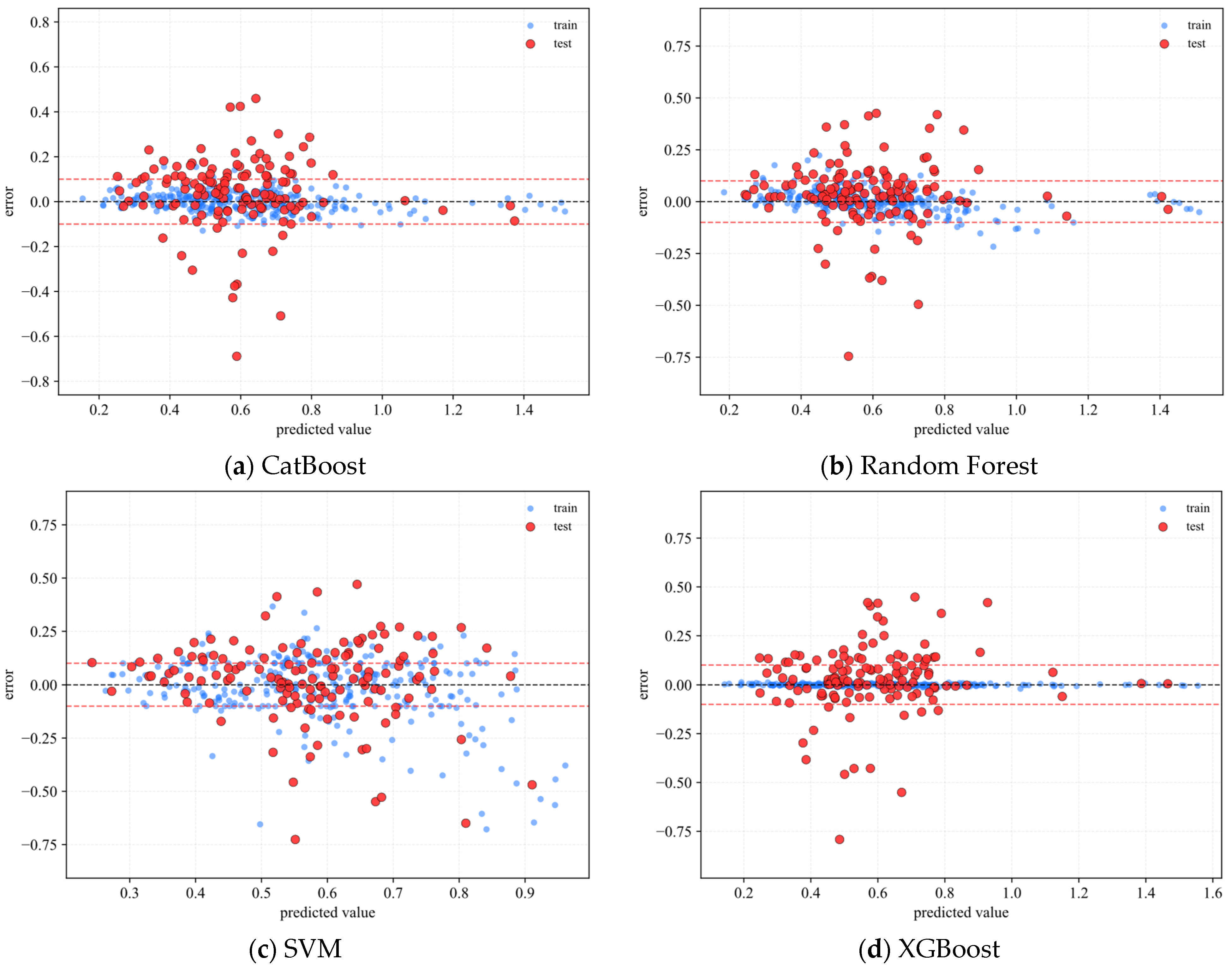
To further illustrate the prediction behavior of different models, one representative train–test split with a random seed of 5 was selected to plot the predicted-versus-observed scatter diagrams and residual distributions. It should be emphasized that these figures are used only for visual interpretation, while the quantitative comparison of model performance is based on the mean and standard deviation obtained from the 10 repeated grouped hold-out validations, as reported in Table 8.

As shown in Figure 8, the four baseline models exhibited different prediction behaviors under the representative grouped train–test split with random seed 5. The SVM model showed relatively scattered prediction points, especially in the medium-to-high water inflow range, indicating limited capability in capturing the complex nonlinear seepage response. XGBoost fitted the training set almost perfectly, with a training R² of 1.000, but its test R² decreased to 0.487 and the test samples were more dispersed, suggesting a clear overfitting tendency.

In comparison, RF and CatBoost achieved more balanced prediction performance. RF obtained training and test R² values of 0.951 and 0.550, respectively, with most prediction points distributed around the ideal diagonal line. CatBoost achieved a training R² of 0.970 and a slightly higher test R² of 0.558, showing comparable fitting stability and slightly better test-set accuracy under this representative split. Overall, the visual results indicate that SVM tended to underfit, XGBoost tended to overfit, whereas RF and CatBoost provided more stable predictions. Among the four baseline models, CatBoost showed the best overall performance in this representative grouped split, which is consistent with the repeated grouped validation results in Table 6. Therefore, CatBoost was selected as the base model for subsequent hyperparameter optimization.

The residual distributions in Figure 9 further support the visual observations from the predicted-versus-observed plots. The SVM model showed relatively scattered residuals, and its predicted values were compressed within a narrow range, indicating limited capability in representing the nonlinear variation in tunnel water inflow. XGBoost exhibited nearly zero training residuals, but its test residuals fluctuated much more significantly, which reflects a clear overfitting tendency under the representative grouped split.

In comparison, RF and CatBoost showed more stable residual distributions. The residuals of RF were generally distributed around the zero-error line, although several test samples still exhibited noticeable deviations. CatBoost also showed a concentrated training residual distribution and a relatively balanced test residual distribution, with no obvious systematic bias. Although some test residuals remained relatively large, CatBoost achieved the highest test R² in the representative split and showed better overall performance in the repeated grouped validation results.

Overall, Figure 8 and Figure 9 indicate that SVM tended to underfit the complex seepage response, XGBoost tended to overfit the training data, and RF and CatBoost provided more reliable predictions. Combined with the statistical results in Table 8, CatBoost demonstrated the best overall balance between prediction accuracy and generalization stability and was therefore selected as the base model for subsequent hyperparameter optimization.

4.2. Performance Comparison of CatBoost Models Optimized by Different Strategies

Based on the repeated grouped validation results of the baseline models, CatBoost was selected as the base model for further hyperparameter optimization. To evaluate the influence of different optimization strategies on CatBoost prediction performance, four optimized CatBoost models were constructed, namely RS-CatBoost, BO-CatBoost, OOA-CatBoost, and GWO-CatBoost. All optimization methods were implemented using the same hyperparameter search space and the same evaluation budget of 200 candidate hyperparameter configurations. For each grouped train–test split, hyperparameter optimization was conducted only within the grouped training set using five-fold grouped cross-validation, and the independent grouped test set was used only for final model evaluation.

As shown in

Table 9. Performance comparison of unoptimized and optimized CatBoost models under ten repeated grouped validations.

Model	Dataset	R2	MAE	RMSE	TIME (s)
Unoptimized CatBoost	Training set	0.9661 ± 0.0036	0.0341 ± 0.0014	0.0451 ± 0.0020	0.41 ± 0.03
	Test set	0.6209 ± 0.0405	0.1084 ± 0.0079	0.1555 ± 0.0085
BO-CatBoost	Training set	0.8813 ± 0.0225	0.0610 ± 0.0054	0.0842 ± 0.0085	164.63 ± 51.33
	Test set	0.6192 ± 0.0427	0.1091 ± 0.0068	0.1559 ± 0.0089
GWO-CatBoost	Training set	0.8852 ± 0.0501	0.0585 ± 0.0134	0.0808 ± 0.0205	174.64 ± 73.26
	Test set	0.6171 ± 0.0267	0.1104 ± 0.0073	0.1565 ± 0.0067
OOA-CatBoost	Training set	0.8918 ± 0.0250	0.0583 ± 0.0069	0.0802 ± 0.0102	159.08 ± 30.25
	Test set	0.6118 ± 0.0507	0.1100 ± 0.0074	0.1573 ± 0.0100
RS-CatBoost	Training set	0.8873 ± 0.0440	0.0583 ± 0.0116	0.0805 ± 0.0177	252.79 ± 15.15
	Test set	0.6197 ± 0.0411	0.1087 ± 0.0069	0.1557 ± 0.0078

, the four optimized CatBoost models exhibited very similar prediction performance on the independent grouped test sets. Among the optimized models, RS-CatBoost achieved the highest average test R² of 0.6197 ± 0.0411, followed closely by BO-CatBoost with 0.6192 ± 0.0427 and GWO-CatBoost with 0.6171 ± 0.0267. OOA-CatBoost obtained a slightly lower average test R² of 0.6118 ± 0.0507. In terms of error metrics, RS-CatBoost achieved the lowest test MAE of 0.1087 ± 0.0069 and the lowest test MAPE of 23.2880 ± 2.8012 among the optimized models, whereas BO-CatBoost achieved the lowest test RMSE of 0.1559 ± 0.0089 among the optimized models. These results indicate that the four optimization strategies produced broadly comparable predictive performance, and no optimized model showed a decisive advantage over the others.

Compared with the unoptimized CatBoost model, however, the optimized CatBoost models did not lead to a clear improvement in grouped test-set prediction performance. The unoptimized CatBoost model achieved the highest average test R² of 0.6209 ± 0.0405 and the lowest average test RMSE of 0.1555 ± 0.0085 among all compared CatBoost models. It also obtained the lowest test MAE of 0.1084 ± 0.0079. Although RS-CatBoost achieved the lowest test MAPE among all models, its test R², MAE, and RMSE were slightly inferior to those of the unoptimized CatBoost model. Therefore, from the perspective of overall prediction accuracy and generalization stability, the unoptimized CatBoost model remained the best-performing model under the repeated grouped validation framework.

The training-set results further show that hyperparameter optimization tended to select more regularized or conservative parameter combinations. The training R² of the unoptimized CatBoost model was 0.9661 ± 0.0036, whereas those of BO-CatBoost, RS-CatBoost, OOA-CatBoost, and GWO-CatBoost were 0.8813 ± 0.0225, 0.8873 ± 0.0440, 0.8918 ± 0.0250, and 0.8852 ± 0.0501, respectively. Similarly, the optimized models had higher training MAE and RMSE values than the unoptimized CatBoost model. These results suggest that the optimization process reduced the fitting degree on the training samples to some extent. However, this reduction in training-set fitting did not translate into improved performance on the independent grouped test sets.

In terms of computational efficiency, the unoptimized CatBoost model required the shortest computational time, with an average time of only 0.41 ± 0.03 s, because no hyperparameter search was involved. Among the optimized models, OOA-CatBoost required the shortest average optimization time of 154.96 ± 28.79 s, followed by BO-CatBoost with 164.17 ± 52.85 s and GWO-CatBoost with 169.46 ± 73.28 s. RS-CatBoost required the longest average time of 244.39 ± 20.01 s. Although OOA-CatBoost showed the highest computational efficiency among the four optimization strategies, its grouped test-set prediction performance was slightly lower than those of RS-CatBoost, BO-CatBoost, and GWO-CatBoost.

Overall, the results in Table 9 indicate that CatBoost itself has strong nonlinear fitting and generalization capability for tunnel water inflow prediction under the current feature system and grouped validation framework. Hyperparameter optimization using RS, BO, OOA, and GWO produced similar grouped test-set performance, but none of the optimized models clearly outperformed the unoptimized CatBoost model. Therefore, the unoptimized CatBoost model was retained as the preferred prediction model in this study, while the optimized CatBoost models were mainly used to analyze the influence of different optimization strategies on model performance and computational cost.

To further examine whether the observed performance differences were statistically significant, paired t-tests were conducted by comparing OOA-CatBoost with the unoptimized CatBoost model and the other optimized CatBoost models using the test results from the ten repeated grouped train–test splits.

As shown in

Table 10. Paired t-test results comparing OOA-CatBoost with the unoptimized and optimized CatBoost models under ten repeated grouped validations.

Metric	Comparison	Mean Improvement	95% CI	Cohen’s dz	Relative Improvement	Win Count	p-Value
Test_R2	OOA-CatBoost vs. CatBoost	−0.0091	[−0.0336, 0.0154]	−0.266	−1.47%	6/10	0.4224
	OOA-CatBoost vs. RS-CatBoost	−0.0079	[−0.0289, 0.0130]	−0.270	−1.28%	4/10	0.4146
	OOA-CatBoost vs. BO-CatBoost	−0.0074	[−0.0194, 0.0046]	−0.441	−1.19%	2/10	0.1966
	OOA-CatBoost vs. GWO-CatBoost	−0.0053	[−0.0314, 0.0208]	−0.145	−0.86%	6/10	0.6577
Test_MAE	OOA-CatBoost vs. CatBoost	−0.0015	[−0.0055, 0.0024]	−0.278	−1.43%	3/10	0.4016
	OOA-CatBoost vs. RS-CatBoost	−0.0013	[−0.0044, 0.0019]	−0.287	−1.16%	3/10	0.3883
	OOA-CatBoost vs. BO-CatBoost	−0.0009	[−0.0032, 0.0014]	−0.266	−0.78%	7/10	0.4213
	OOA-CatBoost vs. GWO-CatBoost	0.0004	[−0.0023, 0.0032]	0.111	0.39%	4/10	0.7335
Test_RMSE	OOA-CatBoost vs. CatBoost	−0.0018	[−0.0068, 0.0033]	−0.250	−1.13%	6/10	0.4502
	OOA-CatBoost vs. RS-CatBoost	−0.0016	[−0.0058, 0.0027]	−0.261	−1.00%	4/10	0.4303
	OOA-CatBoost vs. BO-CatBoost	−0.0014	[−0.0039, 0.0011]	−0.403	−0.90%	2/10	0.2340
	OOA-CatBoost vs. GWO-CatBoost	−0.0008	[−0.0059, 0.0043]	−0.116	−0.53%	6/10	0.7223
Test_MAPE	OOA-CatBoost vs. CatBoost	−0.6462	[−1.7659, 0.4735]	−0.413	−2.81%	3/10	0.2241
	OOA-CatBoost vs. RS-CatBoost	−0.3188	[−1.1452, 0.5075]	−0.276	−1.37%	4/10	0.4055
	OOA-CatBoost vs. BO-CatBoost	−0.0068	[−0.5755, 0.5619]	−0.009	−0.03%	7/10	0.9790
	OOA-CatBoost vs. GWO-CatBoost	0.2095	[−0.4699, 0.8890]	0.221	0.88%	5/10	0.5031

, the paired t-test results indicate that OOA-CatBoost did not significantly outperform the unoptimized CatBoost model or the other optimized CatBoost models on the independent grouped test sets. For Test R², the p-values for OOA-CatBoost compared with CatBoost, RS-CatBoost, BO-CatBoost, and GWO-CatBoost were 0.4224, 0.4146, 0.1966, and 0.6577, respectively, all greater than the significance level of 0.05. The 95% confidence intervals of the mean improvements all included zero, indicating that the observed differences in Test R² were not statistically significant.

The error metrics led to the same conclusion. For Test MAE, the corresponding p-values were 0.4016, 0.3883, 0.4213, and 0.7335. For Test RMSE, the p-values were 0.4502, 0.4303, 0.2340, and 0.7223. For Test MAPE, the p-values were 0.2241, 0.4055, 0.9790, and 0.5031. All these p-values were greater than 0.05, and the corresponding confidence intervals included zero. Therefore, OOA-CatBoost did not produce a statistically significant reduction in prediction errors compared with the unoptimized CatBoost model or the other optimized CatBoost models.

The mean improvements of OOA-CatBoost in Test R² were negative in all comparisons, with relative improvements ranging from −0.86% to −1.47%, indicating slightly lower average Test R² values than the compared CatBoost models. For the error metrics, the mean improvements were very small, and their directions were not consistent across different comparisons. Therefore, the minor differences observed in Table 10 should be interpreted as fluctuations caused by repeated grouped splitting rather than robust performance advantages of a specific optimization strategy.

Overall, the statistical test results suggest that OOA-CatBoost is a feasible CatBoost hyperparameter optimization strategy, but it is not significantly superior to the unoptimized CatBoost model or to RS-, BO-, and GWO-based optimization strategies. Under the current numerical simulation database, input feature system, and case-level grouped validation framework, different CatBoost hyperparameter optimization strategies led to similar generalization performance. This finding further confirms that the baseline CatBoost configuration already provided a robust and efficient prediction model, and that the choice of optimization algorithm played a secondary role in improving test-set performance.

5. Discussion

The results of this study provide a simulation-based evaluation of machine learning models for tunnel water inflow prediction under controlled hydraulic and grouting conditions. It should be emphasized that the database used in this study was generated from numerical simulations within a predefined parameter space. Therefore, the following discussion focuses on the predictive behavior of different models within this simulation-derived dataset, rather than claiming direct engineering reliability for field applications.

The data characteristic analysis indicates that most individual input variables showed weak to moderate linear correlations with simulated water inflow per unit tunnel length. The surrounding rock hydraulic conductivity showed a weak positive correlation with water inflow, with a Pearson correlation coefficient of approximately 0.25, suggesting that higher rock permeability tended to promote groundwater inflow into the tunnel. However, this correlation was not dominant in a linear sense, indicating that water inflow variation was not controlled by a single parameter.

Compared with the grouting-related parameters, the excavation-related variables exhibited more noticeable correlations with water inflow. Excavation distance and excavation-position category, treated as an ordinal descriptor in the correlation analysis, were negatively correlated with water inflow, with correlation coefficients of approximately −0.33 and −0.42, respectively. The grouting ring permeability coefficient, grouting ring thickness, and advance grouting length showed very weak linear correlations with water inflow. These results suggest that the seepage response in the simulation-derived dataset was governed by coupled and potentially nonlinear interactions among geological conditions, grouting parameters, and excavation-position descriptors.

The superior grouped-test performance of CatBoost suggests that ordered boosting and regularized gradient boosting may be better suited to the present nonlinear tabular dataset than SVM and the more aggressively fitted XGBoost model. The predicted-versus-observed plots and residual distributions further support this interpretation. SVM showed dispersed prediction points and residuals, indicating insufficient nonlinear fitting capability, whereas XGBoost produced very small training errors but larger test residual fluctuations, reflecting overfitting to case-specific patterns in the grouped training cases. RF and CatBoost provided more stable predictions, with CatBoost showing a slightly better balance between fitting accuracy and grouped test-set generalization. Nevertheless, this generalization ability should be understood as generalization to unseen numerical simulation cases within the same modeling assumptions and parameter domain, rather than to arbitrary field tunnel projects.

The comparison among RS-CatBoost, BO-CatBoost, OOA-CatBoost, and GWO-CatBoost showed that hyperparameter optimization did not substantially improve the grouped test-set performance of CatBoost. The unoptimized CatBoost model achieved the highest average test R² and the lowest average test RMSE among all CatBoost variants, whereas RS-CatBoost only slightly reduced MAE and MAPE. The optimized CatBoost models showed comparable test-set performance, and none of them consistently outperformed the unoptimized CatBoost model. This suggests that the baseline CatBoost configuration already provided a robust parameter setting for the current simulation-derived dataset.

The lower training R² values of the optimized models indicate that the optimization process tended to select more regularized or conservative parameter combinations. However, this reduction in training-set fitting did not translate into improved performance on the independent grouped test sets. Therefore, under the present dataset and search space, the prediction performance of CatBoost was not mainly limited by hyperparameter configuration. The paired statistical tests further support this interpretation, as the confidence intervals of the OOA-CatBoost improvements crossed zero for all test metrics.

This finding is important for interpreting machine learning results in small- to medium-sized geotechnical datasets. In such datasets, apparent improvements caused by hyperparameter optimization may be affected by data partitioning variability, limited sample size, and the adopted validation strategy. In this study, grouped splitting reduced information leakage between samples derived from the same numerical simulation case. However, grouped validation cannot replace external validation using field monitoring data or truly independent benchmark cases. It only provides a stricter internal validation strategy for evaluating model behavior within the simulation-generated database.

From the perspective of computational efficiency, the unoptimized CatBoost model required much less computational time than the optimized models because no hyperparameter search was involved. Among the optimized models, OOA-CatBoost showed relatively low computational cost, but its test prediction performance was slightly lower than those of RS-CatBoost, BO-CatBoost, and GWO-CatBoost. Considering prediction accuracy, statistical robustness, and computational cost, the unoptimized CatBoost model was retained as the preferred model within the present simulation-based study.

The present study has several limitations. First, the database was constructed entirely from numerical simulations under idealized boundary conditions and steady-state seepage assumptions. Although this enables controlled analysis of hydraulic and grouting parameters, it cannot fully represent the heterogeneity, anisotropy, construction disturbance, and uncertainty of real rock masses. Second, the parameter space was limited to the selected ranges of grouting ring permeability, grouting ring thickness, surrounding rock permeability, advance grouting length, and excavation-position descriptors. The model performance outside these parameter ranges remains unknown. Third, although 425 samples were obtained, they were generated from only 25 orthogonal simulation cases at different excavation positions. Therefore, these samples should not be interpreted as 425 independent field cases. Fourth, important hydrogeological and geological factors, such as groundwater level, fault width, fracture density, water pressure, lithological heterogeneity, and transient excavation effects, were not explicitly included.

Therefore, the proposed CatBoost-based prediction framework should be regarded as a simulation-based preliminary assessment tool rather than a validated field prediction model. Before practical engineering application, the framework should be further validated and calibrated using field monitoring data, independent tunnel cases, or benchmark datasets from different geological conditions. Future work should expand the database by incorporating transient seepage simulations, more geological variables, and field-measured water inflow records. Physics-informed machine learning or hybrid modeling approaches that combine numerical simulation, monitoring data, and prior engineering knowledge may further improve model interpretability and external generalization ability.

6. Conclusions

In this study, a simulation-derived database of water inflow per unit tunnel length containing 425 valid samples was established through orthogonal numerical simulations based on a three-dimensional steady-state seepage model incorporating a grouting ring. Four baseline machine learning models and four CatBoost hyperparameter optimization strategies were evaluated under a repeated grouped validation framework. The main conclusions are as follows:

• The selected input variables have clear physical meanings within the numerical seepage model. Pearson correlation analysis showed that most individual variables had weak to moderate linear correlations with simulated water inflow. The surrounding rock hydraulic conductivity showed a weak positive correlation with water inflow, with a coefficient of approximately 0.25, whereas excavation distance and excavation-position category showed more noticeable negative correlations, with coefficients of approximately −0.33 and −0.42, respectively. These results indicate that water inflow variation in the present simulation-derived dataset cannot be explained by a single linear factor and is more likely governed by coupled nonlinear interactions among geological, grouting, and excavation-related variables.
• Under the repeated grouped validation framework, CatBoost achieved the best overall baseline prediction performance among SVM, RF, XGBoost, and CatBoost. Based on ten repeated grouped hold-out validations, CatBoost obtained an average test R² of 0.6209 ± 0.0405, MAE of 0.1084 ± 0.0079, and RMSE of 0.1555 ± 0.0085. RF showed the second-best test performance, XGBoost exhibited a clear overfitting tendency, and SVM showed insufficient fitting capability. These results indicate that CatBoost was the most suitable baseline model for the present simulation-derived dataset and selected feature system.
• Hyperparameter optimization using RS, BO, OOA, and GWO did not substantially improve the grouped test-set performance of CatBoost. The unoptimized CatBoost model achieved the highest average test R² and the lowest RMSE, whereas RS-CatBoost only slightly reduced MAE and MAPE. Considering accuracy, stability, and computational efficiency, the unoptimized CatBoost model provided the best overall performance.
• The statistical comparison showed that OOA-CatBoost did not significantly outperform the unoptimized CatBoost model or the other optimized CatBoost models. For Test R², MAE, RMSE, and MAPE, the paired t-test p-values were all greater than 0.05, and the 95% confidence intervals of the mean improvements included zero. Therefore, OOA should be interpreted as a feasible CatBoost optimization strategy rather than a statistically superior optimization method under the current dataset and validation framework.
• The repeated grouped validation framework helped reduce information leakage caused by samples derived from the same numerical simulation case. By assigning all samples from the same simulation case exclusively to either the training set or the test set, the evaluation provided a stricter assessment of model generalization to unseen simulation cases within the same parameter space. However, this framework does not constitute external engineering validation. The obtained results should therefore be interpreted as evidence of model performance within the simulation-generated database, not as proof of practical reliability in real tunnel projects.

Overall, CatBoost can serve as a promising simulation-based prediction model for tunnel water inflow under the parameter ranges and assumptions considered in this study. Nevertheless, the proposed framework remains preliminary from an engineering application perspective. Field monitoring data, independent tunnel cases, and broader geological conditions are required for further validation before the model can be used as a reliable engineering prediction tool. Future studies should combine numerical simulation data with field measurements, expand the parameter space, and incorporate transient seepage and geological uncertainty to improve external generalization and practical applicability.

References

1. Frenelus, W.; Peng, H.; Zhang, J. Evaluation methods for groundwater inflows into rock tunnels: A state-of-the-art review. Int. J. Hydrol. 2021, 5, 152–168. [Google Scholar] [CrossRef]
2. Mahmoodzadeh, A.; Mohammadi, M.; Gharrib Noori, K.M.; Khishe, M.; Hashim Ibrahim, H.; Farid Hama Ali, H.; Nariman Abdulhamid, S. Presenting the best prediction model of water inflow into drill and blast tunnels among several machine learning techniques. Autom. Constr. 2021, 127, 103719. [Google Scholar] [CrossRef]
3. Huang, Z.; Yang, Z.; Wu, Y.; Ma, L.; Sun, T.; Wang, Z.; Zhao, K.; Zhang, X.; Li, H.; Zheng, Y. Improving a Prediction Model for Tunnel Water Inflow Estimation Using LSTM and Bayesian Optimization. Water 2025, 17, 3045. [Google Scholar] [CrossRef]
4. Mahmoodzadeh, A.; Ghafourian, H.; Hussein Mohammed, A.; Rezaei, N.; Hashim Ibrahim, H.; Rashidi, S. Predicting tunnel water inflow using a machine learning-based solution to improve tunnel construction safety. Transp. Geotech. 2023, 40, 100978. [Google Scholar] [CrossRef]
5. Yao, X.; Huang, M.; Shi, F.; Yu, L.; Fang, Y. Intelligent prediction of tunnel water inflow during construction based on feature optimization and two-stage ensemble learning. Eng. Appl. Artif. Intell. 2026, 171, 114247. [Google Scholar] [CrossRef]
6. Zhang, N.; Niu, M.; Wan, F.; Lu, J.; Wang, Y.; Yan, X.; Zhou, C. Hazard Prediction of Water Inrush in Water-Rich Tunnels Based on Random Forest Algorithm. Appl. Sci. 2024, 14, 867. [Google Scholar] [CrossRef]
7. Zhou, J.; Zhang, Y.; Li, C.; Yong, W.; Qiu, Y.; Du, K.; Wang, S. Enhancing the performance of tunnel water inflow prediction using Random Forest optimized by Grey Wolf Optimizer. Earth Sci. Inform. 2023, 16, 2405–2420. [Google Scholar] [CrossRef]
8. Zheng, S.; Zhang, Q.; Yang, Y.; Liu, X. Research and application of reliability evaluation model for water inrush risk during tunnel construction. Tunn. Undergr. Space Technol. 2026, 168, 107121. [Google Scholar] [CrossRef]
9. Liu, Y.; Chen, H.; Zhang, L.; Wang, X. Risk prediction and diagnosis of water seepage in operational shield tunnels based on random forest. J. Civ. Eng. Manag. 2021, 27, 539–552. [Google Scholar] [CrossRef]
10. Ju, S.; Ou, G.; Peng, T.; Wang, Y.; Song, Q.; Guan, P. Tunnel water inflow prediction using explainable machine learning and augmented partially missing dataset. Front. Earth Sci. 2025, 13, 1590203. [Google Scholar] [CrossRef]
11. Han, G.; Sheng, J.; Han, R.; Wang, H. Physics-inspired dynamic boosting framework for capturing water and mud inrush evolution in tunnel fault fracture zones. Tunn. Undergr. Space Technol. 2025, 166, 106973. [Google Scholar] [CrossRef]
12. Peng, Y.; Zhang, S.; Su, L.; Yao, Z. Risk Prediction of Water Inrush in Diversion Tunnel Crossing Water-Rich Fault Based on NRBO-XGBoost Algorithm. Appl. Sci. 2026, 16, 3831. [Google Scholar] [CrossRef]
13. Cui, J.; Wu, S.; Cheng, H.; Hou, X.; Wang, J.; Liu, W.; Chu, C. An interpretable and adaptive tunnel water inflow prediction method using data augmentation and AHP-Enhanced OP-LightGBM. Tunn. Undergr. Space Technol. 2026, 171, 107445. [Google Scholar] [CrossRef]
14. Wang, M.; Zhang, J.; Li, H.; Zhang, B.; Yang, Z. Identification of mine water source based on TPE-LightGBM. Sci. Rep. 2024, 14, 12539. [Google Scholar] [CrossRef] [PubMed]
15. Shi, J.; Wang, S.; Qu, P.; Shao, J. Time series prediction model using LSTM-Transformer neural network for mine water inflow. Sci. Rep. 2024, 14, 18284. [Google Scholar] [CrossRef] [PubMed]
16. Yang, S.; Lian, H.; Xu, B.; Thanh, H.V.; Chen, W.; Yin, H.; Dai, Z. Application of robust deep learning models to predict mine water inflow: Implication for groundwater environment management. Sci. Total Environ. 2023, 871, 162056. [Google Scholar] [CrossRef] [PubMed]
17. Zheng, Q.; Wang, C. Cross-Scenario Interpretable Prediction of Coal Mine Water Inrush Probability: An Integrated Approach Driven by Gaussian Mixture Modeling with Manifold Learning and Metaheuristic Optimization. Symmetry 2025, 17, 1111. [Google Scholar] [CrossRef]
18. Yong, Y.; Jing, L.; Jing, Z.; Yang, L.; Li, Z.; Ruxue, G. Application of light gradient boosting machine in mine water inrush source type online discriminant. Int. J. Comput. Sci. Eng. 2021, 24, 9–17. [Google Scholar] [CrossRef]
19. Yao, X.; Huang, M.; Shi, F.; Yu, L. Intelligent and Sustainable Classification of Tunnel Water and Mud Inrush Hazards with Zero Misjudgment of Major Hazards: Integrating Large-Scale Models and Multi-Strategy Data Enhancement. Sustainability 2025, 17, 11286. [Google Scholar] [CrossRef]
20. Xu, Z.; Kong, F.; Cao, C.; Zhang, Z. Prediction and analysis of tunnel water inrush disasters in Chinese Karst area based on Variable weight-weighted Bayesian network model. Carbonates Evaporites 2024, 40, 2. [Google Scholar] [CrossRef]
21. Duan, B.; Chu, A.; Bu, L.; Li, Z.; Long, K. Safety Risk Evaluation of Water and Mud Inrush in Karst Tunnel Based on an Improved Weighted Cloud Model. Sustainability 2025, 17, 9328. [Google Scholar] [CrossRef]
22. Dong, L.; Wang, Q.; Zhang, W.; Zhang, Y.; Li, X.; Liu, F. Risk assessment of tunnel water inrush based on Delphi method and machine learning. Front. Earth Sci. 2025, 13, 1555493. [Google Scholar] [CrossRef]
23. Lei, W.; Han, J.; Wu, X. Improved Osprey Optimization Algorithm with Multi-Strategy Fusion. Biomimetics 2024, 9, 670. [Google Scholar] [CrossRef] [PubMed]
24. Zhang, Y.; Zhou, J.; Li, J.; He, B.; Armaghani, D.J.; Huang, S. Advancing overbreak prediction in drilling and blasting tunnel using MVO, SSA and HHO-based SVM models with interpretability analysis. Geomech. Geophys. Geo-Energy Geo-Resour. 2025, 11, 53. [Google Scholar] [CrossRef]
25. Li, X.; Zhang, C.; Wang, B.; Yang, J.; Wen, Z.; Geng, S. Parameter Inversion of Water Injection-Induced Fractures in Tight Oil Reservoirs Based on Embedded Discrete Fracture Model and Intelligent Optimization Algorithm. Processes 2026, 14, 1176. [Google Scholar] [CrossRef]
26. Shang, R.; Yang, Y.; Huang, B.; Chen, Y.; Qiu, C.; Liu, W. Calibration and intelligent optimization for DEM numerical parameters in heterogeneous rock mass. Comput. Geotech. 2025, 177, 106863. [Google Scholar] [CrossRef]
27. Schober, P.; Boer, C.; Schwarte, L.A. Correlation Coefficients: Appropriate Use and Interpretation. Anesth. Analg. 2018, 126, 1763–1768. [Google Scholar] [CrossRef] [PubMed]
28. Ran, X.; Xi, Y.; Lu, Y.; Wang, X.; Lu, Z. Comprehensive survey on hierarchical clustering algorithms and the recent developments. Artif. Intell. Rev. 2023, 56, 8219–8264. [Google Scholar] [CrossRef]
29. Sujon, K.M.; Hassan, R.B.; Towshi, Z.T.; Othman, M.A.; Samad, M.A.; Choi, K. When to Use Standardization and Normalization: Empirical Evidence From Machine Learning Models and XAI. IEEE Access 2024, 12, 135300–135314. [Google Scholar] [CrossRef]
30. Khoshvaght, H.; Permala, R.R.; Razmjou, A.; Khiadani, M. A critical review on selecting performance evaluation metrics for supervised machine learning models in wastewater quality prediction. J. Environ. Chem. Eng. 2025, 13, 119675. [Google Scholar] [CrossRef]
31. Dehghani, M.; Trojovsky, P. Osprey optimization algorithm: A new bio-inspired metaheuristic algorithm for solving engineering optimization problems. Front. Mech. Eng. 2023, 8, 1126450. [Google Scholar] [CrossRef]
Figure 1. Three-dimensional geological seepage model and mesh discretization.
Applsci 16 06882 g001
Figure 2. Comparison of water pressure distributions at 0.2 m above the tunnel crown under different mesh densities.
Applsci 16 06882 g002
Figure 3. Relationship between permeability coefficient and flow rate under fixed hydraulic boundary conditions.
Applsci 16 06882 g003
Figure 4. Calculation positions for water inflow per unit tunnel length along the tunnel axis.
Applsci 16 06882 g004
Figure 5. Distribution of simulated water inflow per unit tunnel length.
Applsci 16 06882 g005
Figure 6. Pearson correlation matrix among the selected input variables and water inflow per unit tunnel length.
Applsci 16 06882 g006
Figure 7. Technical roadmap of CatBoost hyperparameter optimization under the repeated grouped validation framework.
Applsci 16 06882 g007
Figure 8. Representative predicted-versus-observed plots of baseline models under one grouped train–test split with random seed 5. The brown and blue points represent the training and test datasets, respectively, and the dashed line denotes the 1:1 reference line between the true and predicted values.
Applsci 16 06882 g008
Figure 9. Representative residual distributions of baseline models under one grouped train–test split with random seed 5. The dashed horizontal lines indicate the ±0.10 error bounds used to visually assess the residual distribution. The blue and red points represent the training and test datasets, respectively.
Applsci 16 06882 g009